Land Degradation States and Trends in the Northwestern Maghreb Drylands, 1998–2008

Abstract

States of ecological maturity and temporal trends of drylands in Morocco, Algeria and Tunisia north of 28°N are reported for 1998–2008. The input data were Normalized Difference Vegetation Index databases and corresponding climate fields, at a spatial resolution of 1 km and a temporal resolution of one month. States convey opposing dynamics of human exploitation and ecological succession. They were identified synchronically for the full period by comparing each location to all other locations in the study area under equivalent aridity. Rain Use Efficiency (RUE) at two temporal scales was used to estimate proxies for biomass and turnover rate. Biomass trends were determined for every location by stepwise regression using time and aridity as predictors. This enabled human-induced degradation to be separated from simple responses to interannual climate variation. Some relevant findings include large areas of degraded land, albeit improving over time or fluctuating with climate, but rarely degrading further; smaller, but significant areas of mature and reference vegetation in most climate zones; very low overall active degradation rates throughout the area during the decade observed; biomass accumulation over time exceeding depletion in most zones; and negative feedback between land states and trends suggesting overall landscape persistence. Semiarid zones were found to be the most vulnerable. Those results can be disaggregated by country or province. The combination with existing land cover maps and national forest inventories leads to the information required by the two progress indicators associated with the United Nations Convention to Combat Desertification strategic objective to improve the conditions of ecosystems and with the Sustainable Development Goal Target 15.3 to achieve land degradation neutrality. Beyond that, the results are also useful as a basis for land management and restoration.

1. Introduction

The Maghreb spans northwest Africa from the Mediterranean Sea to the Sahara Desert. Its name refers to the western part under Arab influence and includes Tunisia, Algeria and Morocco. A substantial fraction of the regional landscape of these countries, with a combined area of ~3,000,000 km² and supporting over 80 million people, is drylands.

Several factors have traditionally impeded the estimation of landscape states and trends in the Maghreb, some of which are shared by other drylands around the world. They include a climate often defined better by variance than averages, inherent low ecological productivity and, nonetheless, a mosaic of socioeconomic activities in which extensive nomadic exploitation of rangelands is combined with intensive crop management around stable water resources. However, the Maghreb countries have undergone dynamic changes since gaining independence from colonial rule and are now a region of emerging economic importance. Deeply-rooted traditional knowledge colliding with modern land use practices has brought about new challenges, which have become specific drivers of land degradation. These include population growth, improper management of arable land and overgrazing, and these often occur under adverse climate conditions, such as droughts, intense rainfall events and associated floods. Changes in land use associated with new technological and agricultural developments, such as machinery for perforating boreholes, ploughing hillslopes or road transport of livestock, are considered to worsen rather than improve the long-term capacity of the region’s landscape to provide sustainable resources for the local population.

The long-term framework of this study is the series of projects on global degradation assessment, which started late in the last century, including the Global Assessment of Human-Induced Soil Degradation (GLASOD) [1], the Land Degradation Assessment in Drylands (LADA) [2] and the Global Assessment of Land Degradation and Improvement (GLADA) [3]. This has involved progression toward greater integration, as exemplified by the substitution of the term ‘soil’ by ‘land’ as a target subject, the explicit consideration of ecosystem functions to define degradation and the inclusion of socio-economic drivers, carbon balance and biodiversity as components of the functional land system and its degradation.

This progression was consolidated in the United Nations Convention to Combat Desertification (UNCCD) Decadal Strategy 2008–2018, one of the strategic targets of which is to improve ecosystem conditions. Advance is to be measured by two progress indicators, land productivity trends and land cover trends. Candidate metrics for these indicators are currently being tested and mostly address monitoring procedures, such as those used in GLADA and the new World Atlas of Desertification [4]. At the same time, independent initiatives have been developed in the same direction, often focused on an ecosystemic approach to land degradation emphasizing higher resolution and relative, rather than absolute estimation of ecosystem functioning [5]. The present study forms part of such an initiative and targets the gap in reliable land degradation diagnostics, which can be consistently compared worldwide and replicated over time [6]. This context places strong emphasis on determining productivity trends under the assumption that continuous monitoring of an ecosystem function leads to meaningful assessment of its overall state. However, this assumption poses some limitations.

First of all, a trend is a flow-type variable. It should be used along with its corresponding level-type variable to yield an interpretable picture. In the case of productivity, the associated level variable targets biomass. Telling active degradation from the final stages of a secondary ecological succession, or agricultural intensification from initial succession stages, is only possible by considering both productivity and biomass.

Secondly, monitoring and assessment should be approached separately in many environmental sciences. This is because monitoring refers to the regular observation of a natural phenomenon and often uses absolute rates of change, whilst assessment addresses the position of an element (e.g., a piece of land) within the range of all of its comparable elements and often uses relative estimators. It is not usually meaningful to compute only rates of change of relative measures. A recent example of this is the yet unsettled controversy on land degradation trends in the Sahel using rain use efficiency (a relative index) as a main variable [7,8,9,10].

In this study, land condition refers to the position of a given piece of land on a scale of ecological maturity as defined by ecological succession. It consists of a range of states resulting from often opposing dynamics of ecological self-organization and human exploitation. Land may change state over time, and hence, trends must also be reported.

Land degradation is a subset of land conditions, which is why this study deals with the latter, more general concept. Paradigms underlying its estimation are normally based on some ecological function that evolves in parallel with land degradation or improvement processes [11]. Soil productivity, and more specifically, Aboveground Net Primary Productivity (ANPP, i.e., the rate of change of epigean biomass over time), is an early indicator of an ongoing change in soil function, and therefore, the UNCCD defines land degradation as a ‘reduction or loss in arid, semi-arid and dry sub-humid areas of biological or economic productivity and complexity’.

Today’s accepted approach to land condition surveys resorts to archived time series of vegetation index data and associated climate fields [12]. The integral over a time span of a vegetation density index, such as the Normalized Difference Vegetation Index (NDVI), is an established surrogate for ANPP [13,14]. However, raw ANPP is a poor indicator in drylands because of its strong dependence on soil water availability, and its ratio to precipitation over a given period is preferred. Formulated this way, Rain Use Efficiency (RUE) [15] is an appropriate indicator of land condition, because it is an efficiency ratio in which the green biomass output is relative to rainfall input. High RUE means a well-developed soil-supporting vegetation functioning between sparse rainfall events. It also implies that most of the water is lost to the atmosphere vertically rather than horizontally through runoff.

The use of RUE for assessing land degradation has become an established approach since it was applied for the first time in the Sahel [7]. Studies using satellite imagery as input data have recently been carried out in the Sahel [8,9], Patagonia [16,17] and Inner Mongolia [18,19], to cite just a few. However, direct application of RUE poses some limitations, as discussed in Section 2.2 below. With respect to the determination of trends, the approach of separating simple climate effects from human-induced land degradation [20] meant a tipping point in the detection of true degradation processes, as demonstrated by recent applications [21,22]. The associated RESTREND technique first fits a linear regression to account for climate effects on NDVI and then, using its residuals, identifies non-climate trends to be interpreted in terms of degradation. However, the implicit assumption that climate is always the main predictor of NDVI could be misleading where there is a strong correlation between climate and time [23]. In the present study, this is addressed using stepwise regression, as discussed in Section 2.3.

The NW Maghreb is an important area for land degradation studies, because its contrasting dynamics and complexity challenge the technical issues addressed above when applied on a regional scale. Furthermore, any method involving end users should: (i) base its paradigms on an ecological function; (ii) derive input data from readily available open databases; (iii) neatly separate objective computational processes from expert-driven intervention; and (iv) offer results that are relevant for UNCCD and users alike whilst being ecologically interpretable.

In this study, we have applied a refined methodology, called 2dRUE, which consists of separate assessment and monitoring procedures. It deals with both the limitations and with the stated user constraints described above. This study: (i) makes a diagnosis of the states and trends of land in the drylands of NW Maghreb over a recent ten-year period; (ii) explicitly implements crucial elements of the UNCCD progress indicators dealing with ecosystem condition; and (iii) offers candidate metrics that can be used by the countries concerned and others to report land degradation to the UNCCD. The period of analysis was selected to set a reference level or ‘baseline’ against which the progress of the UNCCD 2008–2018 Strategy can be measured.

2. Materials and Methods

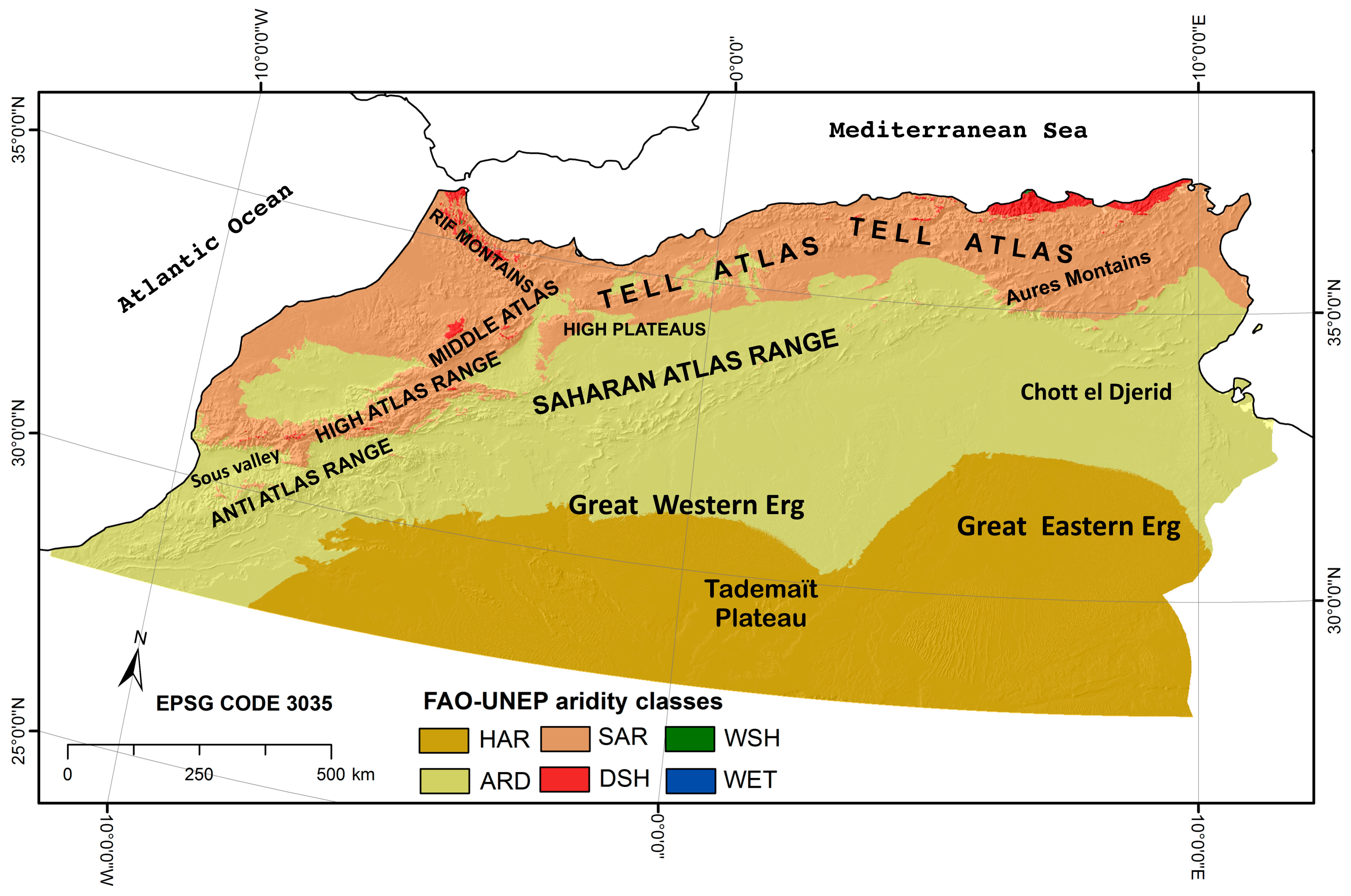
2.1. Study Region

This study focuses on the drylands of Morocco, Algeria and Tunisia north of 28°N (Figure 1). The region lies on a long gradient of aridity between the Mediterranean and Atlantic coasts on one side and the Sahara desert on the other. Data from the climate archive developed for this study show that in terms of the FAO-UNEP aridity classes, the windowed region includes hyper-arid (57%), arid (29%), semi-arid (13%) and dry sub-humid (1%) zones, as well as altitudinal belts with higher humidity in the mountain ranges. The UNCCD definition of ‘areas affected by desertification’ ranges from dry sub-humid to arid zones, all of which are commonly referred to as drylands. From this point of view, the study region includes practically all of the UNCCD target land in Morocco (385,308 km²), Algeria (567,481 km²) and Tunisia (144,174 km²).

The Atlas Mountain Chain crosses the region SW to NE along approximately 2400 km, regularly exceeding 2000 m a.s.l. and marking break points in the dominant NW to SE aridity gradient. North of the High Atlas, Middle Atlas and Tell Atlas ranges, the climate is Mediterranean, with dry summers and predictable cold-season precipitation ranging from about 300–1200 mm, depending on altitude and exposure to synoptic effects. The Tell Atlas and Saharan Atlas Ranges enclose a zone of elevated endorheic plains known as the High Plateaus, where climate is cold, semi-arid Mediterranean. South of the Anti-Atlas and the Saharan Atlas ranges, the Mediterranean influence decreases quickly, and the xeric influence of the Sahara desert becomes dominant, with low precipitation, often below 100 mm and subject to high between-year variability. Mesoforms in this sector include two large sand seas, the Great Western and Great Eastern Ergs, and the rocky Tademaït Plateau just south of the study window.

The physiographic layout described above controls the distribution of human populations and how they have traditionally exploited natural resources. In precolonial times, populations in settlements and nomadic people built a complex network of relationships, with a mixture of positive and negative effects in ecosystems, but with a positive balance for the stability of the whole landscape. Since then, new socioeconomic forces have been reshaping the landscape [24]. Some of the most outstanding are a dramatic increase in population, technological intensification of agriculture north of the Atlas ranges, progressive sedentarization of nomads and migration from rural areas [25,26]. From 1950–2000, urban and rural populations increased by factors of 4 and 3, respectively, because of a dramatic reduction in child mortality, amongst other reasons [27]. The recent trend toward stabilization of the rural population is explained by increased internal and international migration, including the return of ‘reverse’ migrants [28]. The environmental impact has been the expansion of agriculture over poor soils and the degradation of steppes and rangelands.

Mediterranean lowlands north of the Atlas and along the Atlantic coast sustain most of the productive regional agriculture, either rainfed or by irrigation canal networks, which support densely-populated centers of intense trading. This is embedded in a matrix of sclerophyllous forests (e.g., Quercus ilex subsp. rotundifolia, Q. suber, Q. coccifera, Pistacia atlantica, Tetraclinis articulata, Argania spinosa), montane forests (e.g., Cedrus atlantica, Abies pinsapo, Juniperus thurifera) and serial shrublands (e.g., Juniperus oxycedrus, Pistacia lentiscus, Ziziphus lotus). Land use here is challenged by general intensification of agriculture, evolving from subsistence to export, with the resulting soil salinization issues and fragmentation of the natural vegetation by firewood extraction and overgrazing.

The High Plateaus form an open treeless steppe with dispersed plant cover on up to 80% of the soil surface, represented by perennial Gramineae, like Macrochloa tenacissima, Stipa spp. Lygeum spartum, Panicum turgidum, Stipagrostis pungens and Stipagrostis spp. Sand accumulation favors patches of Lygos sphaerocarpa, Retama spp. and Tamarix spp., and vegetation in endorheic depressions (daïas) is represented by Pistacia atlantica and Ziziphus lotus [29]. The High Plateaus have a sparse human population and have traditionally been used for transhumant grazing. In recent times, such activity has intensified with semi-permanent sheds and transport of animals in lorries, increasing livestock [30]. The overall balance has been reported as widespread, mostly irreversible, degradation of grasslands and loss of productivity in the range of 20%–40% during the last few decades [27,31].

The vegetation strategy undergoes a change in the hyper-arid domain. It has its own characteristics and was not included in this study; firstly, because adaptive traits of vegetation to extreme aridity differ from those of relatively wetter zones, and therefore, an assessment based on productivity and turnover ratio was not likely to yield meaningful results; secondly, to properly include the hyper-arid domain, a much larger study area, beyond this study’s regional scope, would have been necessary; and thirdly, hyper-arid zones are not included in the UNCCD definition of drylands, which are the target of this study.

2.2. Methods

The 2dRUE empirical method was used for this work. Its rationale, assumptions and algorithms are described in depth elsewhere [23], and a brief video presentation showing its highlights and some user-level examples is available [32]. The method has been coded as a free open source library of functions in R: r2dRue [33]. Therefore, only a summary and the new revised procedure for generating the assessment and monitoring map legends are given below.

2.2.1. Background on 2dRUE

The simple application of RUE involves certain problems that should be considered before using it for surveying the land condition in large territories: (a) an RUE sequence cannot be monitored using precipitation as a denominator because of the interannual variability of rainfall; (b) similarly, due to its formulation, the direct comparison of zones where aridity is very different is not possible either; (c) it follows from the above that the designation of reference areas with optimum RUE is far from obvious; and (d) a single implementation of annual RUE is an excessive generalization of vegetation performance. The 2dRUE method deals with those issues below.

To solve Problem a described above, assessment and monitoring are performed separately for the same time period. For Problem d, assessment is made based on two implementations of RUE, one long term, on an annual average scale as a proxy of overall biomass and maturity, and another short term for the single six-month period before maximum vegetation density for the whole period of analysis as a proxy for productivity and resilience. These observed RUEs are then corrected using an aridity index to deal with Problem b above, yielding two corresponding RUE estimates, both of which are relative to the minimum and maximum potential RUE for any aridity (Problem c). These are direct indicators of the condition state in two complementary dimensions. The assessment therefore compares each location to all other locations across the study area.

Because of Problem a above, RUE cannot be used for monitoring, and biomass change over time (i.e., annual NDVI means) is used instead. However, simply monitoring vegetation density over the course of time compounds two important factors that should be separated. Vegetation may change over time due to drifting between-year rainfall or intrinsic ecological trends [20]. Only after having separated them can the latter be interpreted in terms of ongoing ecological succession or human-induced degradation, which is the most relevant for monitoring land condition. Therefore, monitoring is done by stepwise regression of annual vegetation density over time and aridity. This yields two quantitative maps of the effects of these factors on vegetation trends. Monitoring therefore compares each location to itself over time during the period of analysis.

The four quantitative maps are proper indicators and convey the maximum information from this method. However, an effort must be made to approach the UNCCD concept of the progress indicator of ecosystem condition. This is done by combining the two maps of RUE (long and short term) to a map of assessment reflecting land condition states and the two maps of regression effects (time and aridity) to a monitoring map of land condition trends. The participation of users in this process is crucial. However, at the same time, the overall process is transparent for them because any decision to be made and its ecological implications are precisely identified, and the computational procedures are automatic.

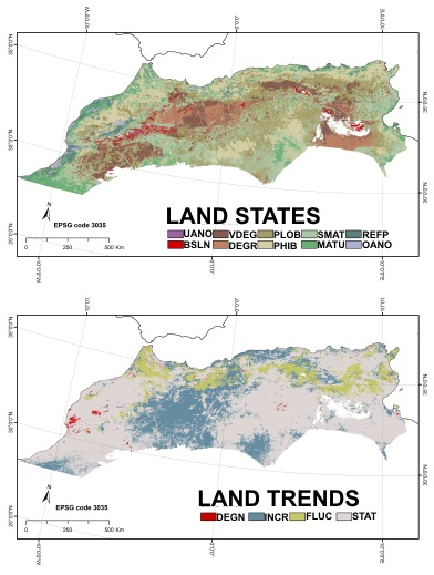
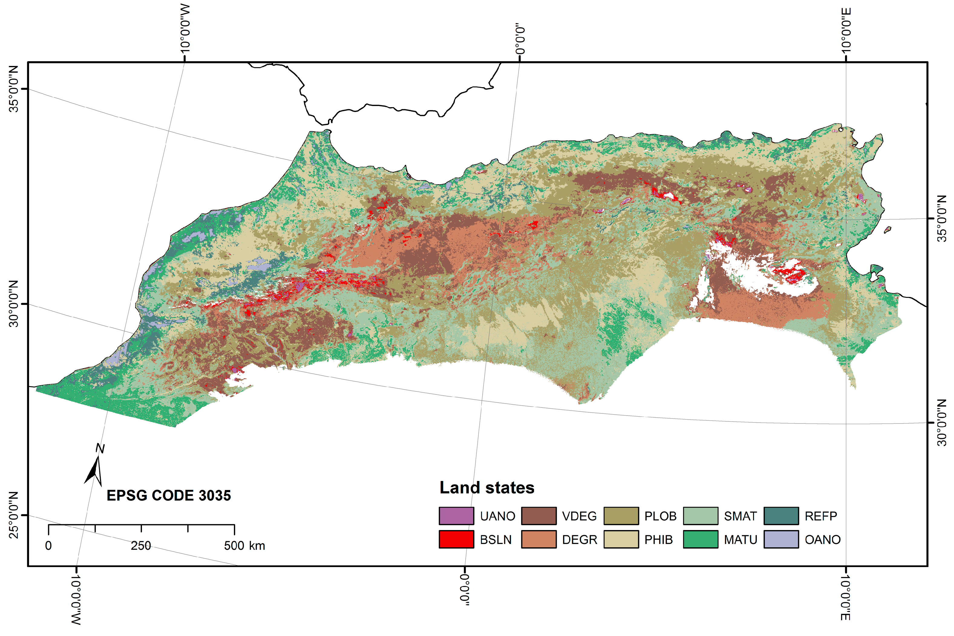
2.2.2. Assessment of Land Condition States

Assessment in 2dRUE relies on scatterplots of observed RUE over a corresponding aridity index, which is defined as the ratio of Potential Evapotranspiration (PET) to precipitation P over the study period. Therefore, two scatterplots were calculated, mean observed RUE (RUE_{OBS_me}) against the mean aridity index (AI_{OBS_me}) and extreme observed RUE (RUE_{OBS_ex}) against the extreme observed aridity index (AI_{OBS_ex}).

The scatterplots show a range of observed RUE for any given aridity. In this simplified framework, their upper and lower boundaries reflect the potential maximum and minimum vegetation performance that can be expected as a function of aridity. The observed RUE for any location is then relativized to its potential boundaries by rescaling it to a range of 0 (if equal to its potential minimum) to 1 (if equal to its potential maximum). Values outside that range are possible because of the statistical detection of boundaries using percentiles.

Mean or extreme relative RUE (rRUE_me or rRUE_ex, respectively) is useful because either maintains the relative positions of all of the locations in the corresponding scatterplot, while the performance is standardized to a common interval. Therefore, a map of relative RUE is corrected for aridity, and distant locations can be directly compared on this basis.

An early implementation of the assessment in the Iberian Peninsula [23] classified vegetation into three groups by whether relative RUE was below, within or above the 0–1 range. This approach was considered acceptable for the Iberian Peninsula, where the ecological history of the land is well known, socioeconomic drivers of land condition are consistently widespread and supporting environmental information is abundant. However, several flaws became apparent after its application to the Maghreb. Firstly, there are vast rangelands in the study region where grazing intensity causes different vegetation responses. The long- and short-term implementations were designed to capture biomass and productivity, respectively. However, by not distinguishing these attributes to define land condition states, that information was lost.

Secondly, the use of rigid rRUE_me or rRUE_ex limits for classifying vegetation performance is perhaps an acceptable simplification, but nonetheless, it leads to inconsistencies. For example, 0.01 and 0.99 would both be classified as ‘within range’, although they are much closer to a potential boundary than to the center of the range. Finally, the within-range class so defined is comprised of the majority of locations, as the boundary functions used to compute relative RUE were fitted using the 5th and 95th percentiles. As a result, large areas of land remain without further detail.

To alleviate the above problems, the following improvements were made to the assessment component (see also Figure 2 for a graphic explanation):

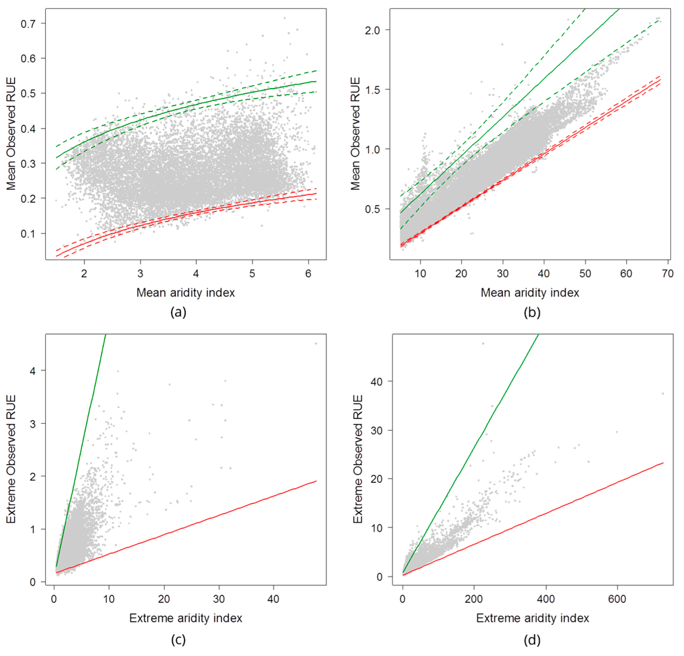
• Semi-arid and more humid zones, on the one hand, and arid zones, on the other, were processed separately in view of their probably different ecological responses to aridity and frequency distributions within the study area. Hyper-arid zones were excluded from the analysis.
• Scatterplot boundary functions were fitted as usual for the long- and short-term implementations. The 1st and 99th percentiles were used to delimit the boundaries. Relative mean and extreme RUE (rRUE_me and rRUE_ex) were then computed.
• Confidence intervals (α = 0.05) were computed for the upper and lower boundary functions of RUE_{OBS_me}. This resulted in a five-zone system in the scatterplot, which provided a basic legend for the assessment map:

  • Underperforming anomaly: Vegetation below the confidence interval of minimum RUE. For example, heavily-disturbed areas.
  • Baseline performance: Vegetation within the confidence interval of minimum RUE. For example, vegetation limited by factors other than rain, such as saline soils.
  • Range: Vegetation between both minimum and maximum RUE confidence intervals. Target class under a variety of uses to be further processed.
  • Reference performance: Vegetation within the confidence interval of maximum RUE. Typically, undisturbed natural vegetation.
  • Over-performing anomaly: Vegetation above the confidence interval of maximum RUE found under rainfed conditions. For example, irrigated crops.
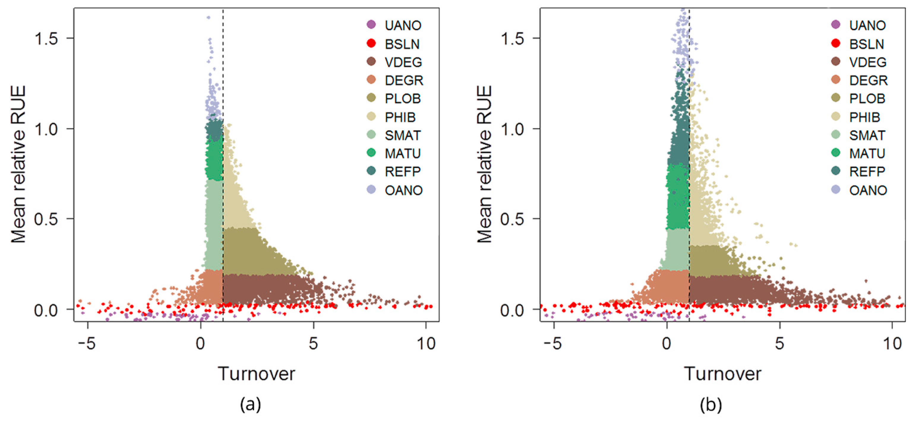
• The Range class was then subdivided using the relative RUE scores in both implementations. Assuming that rRUE_ex and rRUE_me indicate productivity and biomass, respectively, their ratio was taken as a proxy for turnover. The interpretation was therefore in terms of ecological maturity following the rules below:

  • Turnover below 1. Within this subpopulation, rRUE_me:

    • Below the 25th percentile was considered Degraded.
    • From the 25th–75th percentile was considered Submature.
    • Over the 75th percentile was considered Mature.
  • Turnover equal to or greater than 1. Within this subpopulation, rRUE_me:

    • Below the 25th percentile was considered Very degraded.
    • From the 25th–75th percentile was considered Productive with low biomass.
    • Over the 75th percentile rRUE_me was considered Productive with high biomass.
  • An exception was made for the combination (a, i) above in semiarid zones, where the 25th percentile finally used corresponded to that of arid zones. This was done to improve the discrimination of grassland steppes in the plateaus, which lay in a transitional zone between those two levels of aridity.

The Range class is likely to contain locations under active land use, where different responses may be expected from the vegetation cover. We adapted the principles of the ecological theory of succession to formalize an approach to land degradation in rangelands [34,35]. The hypothesis is that annual average biomass may be expected to decrease as land degradation proceeds, whilst productivity would peak at intermediate degradation states. The two RUE implementations used here target these functions respectively, but their observed values cannot be used in comparisons across the study area because of the influence of climate. Therefore, their relative transformations are used for this purpose.

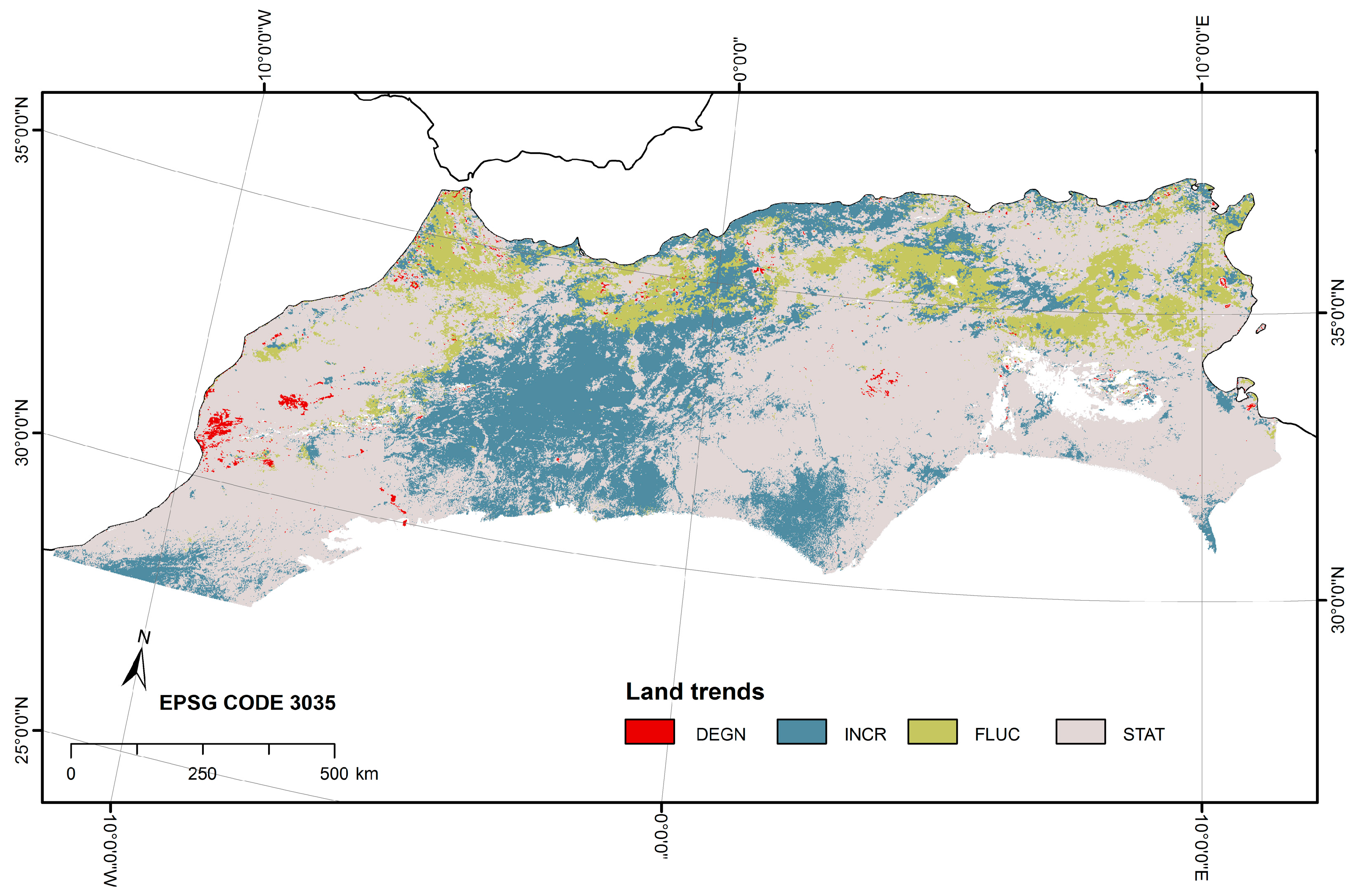
2.2.3. Monitoring Land Condition Trends

Monitoring addresses land trends (irrespective of states) observed during the study period. The effects of between-year variation in aridity and time should be explicitly separated [36]. The first explains resilience to changing rainfall, for example the wetter the year, the greener the vegetation. Once such effects are removed, the accumulation of the depletion of biomass over time is interpreted in terms of ecological self-organization or ongoing degradation.

A standard stepwise regression was done to find comparable effects (i.e., standard partial regression coefficients) of time and aridity on vegetation. Only significant effects (p ≤ 0.10) are reported. Two maps form the primary result of monitoring. The first one is of the effects of between-year variation in aridity (in terms of PET/P) on vegetation. Here, negative values simply mean that vegetation is less green in dry years, and positive values usually refer to increased warming in colder areas. Such trends are lumped together for the study period. The second one is of the effects of time on vegetation. This map conveys long-term vegetation trends after climate drifting has been separated. Positive values typically mean biomass accumulation over time (e.g., a secondary ecological succession after abandonment), whilst negative values indicate some active degradation, either slow (e.g., overgrazing) or sudden (e.g., fire at the end of the period).

Whilst such maps are useful for detailed studies, their respective legends are too complicated to show on the final land condition map. They have therefore been simplified to provide a trend sub-legend:

• Increasing: Biomass accumulation over time, whatever the response to between-year variation in aridity;
• Fluctuating: Biomass fluctuates during the year with aridity, but with no significant variation in the long term;
• Static: No response detected over time, not even to changing aridity within the study period;
• Degrading: Biomass depletion over time, whatever the response to between-year variation in aridity.

2.3. Data

2dRUE is based on archived time series of two main types of input data at a monthly resolution. The first one is a vegetation density index, such as NDVI. The second is a corresponding set of climate fields for mean maximum, mean and mean minimum temperatures and precipitation. A land use/land cover map is also used to mask non-rainfed locations in the computation of scatterplot boundaries, and a vegetation map may be used for the basic interpretation of the results.

2.3.1. Vegetation Density Time Series

The NDVI product SPOT VEGETATION VGT-S10 was used for this work. Data are available free of charge from VITO [37] in geodetic coordinates at a resolution of 0.00892857 degrees from April 1998 forward. A status map layer enables pixels affected by clouds or snow to be masked. The data are delivered in Hierarchical Data Format (HDF).

VGT-S10 consists of a synthesis of single-day mosaics of NDVI data over a ten-day period or dekad (there are conventionally three dekads per month, from Days 1–10, 11–20 and 21 to the end of the month). Such syntheses are atmospherically corrected data of all vegetation segments in a dekad that have been merged into a single image using the Maximum Value Composite (MVC) algorithm, which selects the highest ground reflectance for each pixel. More detailed information can be found in Baret et al. [38].

In this application, each monthly layer was constructed in two steps. First, all pixels in each dekad image with clouds or snow were masked out using the corresponding status map. Second, a single image was made using the maxima detected in the three corresponding dekads. The NDVI time series was then built up by selecting pixels having a valid value for every month from September 1998–August 2008. About 2% of all the pixels in the drylands zone were missing after applying this procedure and were not processed further. The working mask meeting the conditions inclusion in the NDVI time series and in the drylands zone was applied throughout this study.

2.3.2. Climate Archive

A climate archive with the following basic fields was produced for this study: mean maximum, mean and mean minimum temperatures and total precipitation [39,40]. Each field consists of a set of monthly surfaces spanning 1973–2008. The application area covers NW Africa north of 28°N and west of 12°E at a spatial resolution of 0.00833 degrees. These data were used for both basic RUE computation and to produce the potential evapotranspiration component of aridity, following the formula by Hargreaves-Samani [41]. The FAO-UNEP aridity map (Figure 1), computed as the mean annual precipitation to potential evapotranspiration ratio, was used for delimiting drylands in this study. This dataset is freely available [40].

2.3.3. Supplementary Data

The Land Use Systems of the World—North Africa and Near East Version 1.0 [42] was used in this study for masking non-rainfed vegetation. This dataset is a thematic grid of Land Use Systems (LUS) with a spatial resolution of 0.083333 degrees. Agriculture, urban land, wetlands and open water Land Use Systems (LUS) were masked in 2dRUE computations. Masking was conservative because the coarser spatial resolution of this grid excluded potentially valid locations adjacent to these classes.

Elevation data for climate interpolation and the basic geographical layout of the study region were acquired from GLOBE, a global Digital Elevation Model (DEM) at a spatial resolution of 0.0083333 degrees [43].

Country boundaries were extracted from the Digital Chart of the World [44] to acquire land condition statistics by country. The use of such limits in this study does not imply any opinion by the authors concerning their validity.

2.4. Study Period and Spatial Reference

Hydrological years [45] were used to encompass complete annual precipitation and evapotranspiration cycles. Therefore, this study focuses on the period from September 1998–August 2008. Antecedent precipitation in the computation of extreme observed RUE was set to six months. The temporal resolution of the archived time series was one month for assessment and one year for monitoring.

All maps were projected to match the grid and spatial resolution of the NDVI time series, to maintain the integrity of their values and facilitate computation in this and later studies. Therefore, the working Coordinate Reference System (CRS) consists of geodetic coordinates in the WGS84 datum (Code 4326 of the European Petroleum Survey Group (EPSG)). The spatial resolution in degrees equals approximately 1 km within a maximum circle. Two advantages of this procedure are that relevant maps or window regions can be projected onto a target user agency’s CRS with minimum loss of information due to intermediate steps and that the conversion to Keyhole Markup Language (KML) format for interpretation using a suitable web mapping service (e.g., Google Earth) is straightforward at any stage of the work.

In spite of these advantages, a geodetic CRS cannot be represented on flat maps without incurring important distortions of both shape and area, which required the specification of a map projection. For this study, an equal-area projection was appropriate for showing the areas of the different land condition classes in proportion true to their size on the Earth. Thus, the maps presented in this article have been projected onto the Lambert Azimuthal Equal Area system with the European Terrestrial Reference System 1989ETRS89 Datum (EPSG Code 3035). This CRS is the same one used for all of Europe and was selected because of both its seamless connection with other map products of European origin and its potential for extending land condition mapping to other regions around the Mediterranean. The areas reported here were obtained from such projected maps at a spatial resolution of 1 km.

The purpose of this study was to report land condition in UNCCD target ‘affected areas’. Therefore, results in square kilometers for the drylands in the three countries that are the subject of study are reported separately. Beyond this, all statistical tests showing relationships in the results were done using a sample of 42,203 cells (3.93% of the total valid data cells in the study area), extracted by stratified random sampling to avoid spatial autocorrelation.

3. Results

3.1. Land State Determination

The scatterplots of mean and extreme observed RUE over the corresponding aridity estimates used to determine the assessment legend classes (land states) may be seen in Figure 2 and Figure 3.

The experimental results show an increase in mean observed RUE over aridity, which becomes linear in arid zones (Figure 2, Table S1). This is consistent with other findings on convergence to common maximum RUE across different biomes during dry periods [46]. Using time series from sites located throughout North and South America, plots of ANPP over P tended to a common maximum slope when only dry years were included, irrespective of the vegetation zone. Such a slope, also called sensitivity, is RUE by definition. Our results were in a spatial rather than a temporal dimension, but nevertheless, they confirm the increase in RUE over aridity. Extreme RUE follows a similar pattern, but it is computed for a single ANPP peak and for a six-month rainfall period and, therefore, is not comparable to previous studies.

The relationship between biomass (in terms of rRUEme) and turnover (in terms of the rRUEex/rRUEme ratio) conveys the basic land degradation hypothesis explained in Section 2.2. The results are shown in Figure 3. High biomass scores extend over a narrow turnover range below the threshold of one. The lower the biomass, the wider the turnover range in which it may be found. In other words, biomass would be relevant for explaining the states of higher ecological maturity, and turnover would be better for explaining less mature and degraded states.

Figure 3 is simply the graphical expression of the Range class rules described in Section 2.2, not an experimental result. However, out-of-range classes defined using only rRUEme were also plotted, and resulted in being consistent with that interpretation. Reference performance forms a compact patch above Mature, and the scatterplot peaks at Over-performing anomaly. The fact that this class shows a narrow turnover below one suggests the dominant composition of Reference performance outliers and orchards. At the opposite end, Baseline performance lies at the base of the scatterplot and extends over a wide range of turnover values, thereby confirming the interpretation that this class is mostly made up of vegetation limited by factors other than water.

3.2. Land States and Trends in the Drylands

Figure 4 and Figure 5 show maps of land states and trends, respectively, throughout the drylands in the study area and their areas are shown by country and for the whole area in Table S2.

Overall, mid-range land states (Productive with either low or high biomass) were dominant, accounting for 454,880 km² (41% of the drylands domain). Upper-range states (Submature and Mature) follow with 331,232 km² (30%). Lower-range states (Degraded and Very Degraded) were less frequent with 228,070 km² (21%). This pattern, by which better condition states appear to prevail over poorer ones, was also found for the reference states: 37,896 km² (3.45%) of Reference performance were found, whilst only 9130 km² (0.83%) were Baseline performance.

Land states were not randomly distributed among the three countries (

Table 1. Associations of land condition states, land condition trends and countries found using two chi-square tests. Inputs are adjusted residuals (corrected for sample size), expressing differences between observed frequencies and expected frequencies under the null hypothesis of a random distribution. Values are standard deviation units and can be tested as z-scores using a normal distribution. A threshold of ±1.96 was used to determine significance.

Class		Morocco	Algeria	Tunisia
States (χ2 = 3286.60, d.f. = 18, p < 0.0001)	Underperforming anomalies	4.12	−4.73	1.17
	Baseline performance	11.09	−11.85	1.82
	Very degraded	18.99	−7.58	−15.94
	Degraded	2.26	0.71	−4.32
	Productive with low biomass	−26.29	24.87	0.51
	Productive with high biomass	−6.93	4.32	3.48
	Submature	−16.70	4.88	16.69
	Mature	16.68	−16.22	0.35
	Reference performance	31.31	−23.91	−9.18
	Over-performing anomalies	22.52	−17.07	−6.79
Trends (χ2 = 1096.33, d.f. = 6, p < 0.0001)	Degrading	14.32	−11.42	−3.46
	Fluctuating	−8.05	−1.43	13.73
	Increasing	10.92	8.25	−28.07
	Static	−6.91	−4.56	16.77

). Morocco showed a diverging pattern in which its land was positively associated with either poor (e.g., Very Degraded, Degraded) or good (e.g., Mature, Reference performance) condition, whilst intermediate states appeared to be less frequent than would be expected at random. Eastward, the pattern is the opposite in Algeria and Tunisia, where positive associations were found only for intermediate states ranging from Productive with low biomass to Submature.

In contrast to assessment, which is relative, monitoring results are absolute estimates of vegetation trends over time and aridity during the study period. Several findings here are worth mentioning (Table S2). First and foremost, the amount of land actively degrading (degrading) is very low, only 0.7% of the total. On the contrary, much more land (24.1%) is increasing. Fluctuating land covers over 10.8% of the territory. Finally, there is a vast proportion of static land (64.4%) that shows no response over time or aridity.

Like land states, land trends showed significant associations with the three countries (Table 1). Morocco turned out to have proportionally more land undergoing either degrading or increasing trends; Algeria had a positive association only with increasing trends; and Tunisia was found to be associated with both fluctuating and static trends.

Assessment and monitoring procedures operate on the same dataset, but are completely independent exercises in both approach and methods. It is therefore worth asking whether there is any relationship between land states and trends in the drylands of the Maghreb (

Table 2. Association of land condition states (rows) and trends (columns) found using a chi-square test (χ² = 2258.77, d.f. = 27, p < 0.0001). Inputs are adjusted residuals (corrected for sample size), expressing differences between observed frequencies and expected frequencies under the null hypothesis of a random distribution. Values are standard deviation units and can be tested as z-scores using a normal distribution. A threshold of ±1.96 was used to determine significance.

	Degrading	Fluctuating	Increasing	Static
Underperforming anomalies	12.07	0.10	−0.16	−1.91
Baseline performance	0.51	−0.39	5.63	−4.86
Very degraded	−4.07	19.31	4.64	−15.96
Degraded	−4.87	−11.66	24.20	−13.27
Productive with low biomass	−6.09	1.43	−10.95	9.86
Productive with high biomass	2.44	8.85	−20.47	12.16
Submature	0.77	−10.65	10.24	−2.39
Mature	2.36	−6.08	5.99	−1.81
Reference performance	7.41	−1.89	−10.59	9.45
Over-performing anomalies	13.62	−3.24	−5.67	4.90

).

Several facts are apparent after examining the sign and magnitude of residuals. Very degraded, and Degraded states are consistently associated with increasing trends and rarely go on to further degradation. Both types of Productive land appear not to show any trend whatsoever (positive association with static) and with strong resistance to increasing trends. Its response to degrading trends apparently depends on biomass, negative for Productive with low biomass and positive for Productive with high biomass. Submature and Mature states show positive associations with degrading (albeit non-significant in the case of the former) and also with increasing trends, while rarely found to be fluctuating or static. Finally, Reference performance land was found to prevail under degrading or static trends, very rarely under increasing trends.

Aridity zones within the drylands were significantly associated with both land condition states and trends (

Table 3. Associations of land condition states, land condition trends and aridity zones (dry lands) found using two chi-square tests. Inputs are adjusted residuals (corrected for sample size), expressing differences between observed frequencies and expected frequencies under the null hypothesis of a random distribution. Values are standard deviation units and can be tested as z-scores using a normal distribution. A threshold of ±1.96 was used to determine significance.

Class		Arid	Semi-Arid	Dry Sub-Humid
States (χ2 = 2377.47, d.f. = 18, p < 0.0001)	Underperforming anomalies	−3.56	3.91	−1.31
	Baseline performance	−3.70	2.99	3.15
	Very degraded	3.41	−1.66	−7.47
	Degraded	27.58	−26.62	−5.20
	Productive with low biomass	−2.54	5.09	−10.57
	Productive with high biomass	−28.49	28.50	1.22
	Submature	17.13	−17.64	1.37
	Mature	−10.42	6.71	16.01
	Reference performance	1.22	−4.70	14.52
	Over-performing anomalies	−8.38	8.68	−0.90
Trends (χ2 = 2981.48, d.f. = 6, p < 0.0001)	Degrading	−6.96	5.87	4.85
	Fluctuating	−53.75	52.47	7.71
	Increasing	13.28	−13.07	−1.47
	Static	24.04	−23.22	−4.47

). Arid land showed positive associations with Very degraded and Degraded states, but with increasing or static trends. Semi-arid land was associated with a variety of states, notably Productive with high biomass and with degrading or fluctuating trends. Dry sub-humid land resulted in being strongly associated with Mature and Reference performance states, again under degrading and fluctuating trends.

4. Discussion

4.1. Evaluation of the Assessment

Land states were found by statistical calculation using uncalibrated NDVI data, and these two aspects control how the results may be used. They should therefore be examined prior to any further interpretation.

The use of NDVI as a proxy for vegetation density in areas with sparse cover may be a controversial cornerstone of the input data used here. This derives from the very computation of the index using red and near-infrared bands of the spectrum, which makes it particularly sensitive on dry and hyper-arid lands, where soil surface temperature drives sensible heat flux, a large component of the energy balance. A higher index response causing overestimation of vegetation density in desert areas has been reported [47].

Several alternative indexes have been devised to circumvent this problem, such as the Soil-Adjusted Vegetation Index (SAVI) [48], the Green Vegetation Fraction (GVF) [49] and the Fraction of Absorbed Photosynthetically-Active Radiation (FAPAR) [50]. However, proper computation usually requires either fieldwork in sample areas that compromise the representativeness of the overall study or complex statistical modelling, which lends itself to additional errors. It could be for those reasons that the NDVI has become an established product readily available from many sources and is still a staple for regional studies worldwide [10,51,52].

In the work reported here, NDVI shows consistent decline over aridity. False vegetation signals should remain stable over time. However, the proportion of non-static trends in the arid zones was quite relevant, and all of them were well beyond the threshold for being considered random occurrences (Table 3). The immediate implication is that NDVI seems to have captured the dominant spatial-temporal patterns of vegetation in the region successfully, at least within the methodology’s permissible margins of error.

A second point concerning the method is that assessment was relative. In 2dRUE, every location is assessed with respect to a minimum and maximum reference (Baseline and Reference performance, respectively) found empirically for its aridity level. The use of extreme percentiles in this task has two effects. First, few locations fall within either of those classes, as controlled by their respective confidence intervals, even if other similar locations exist in the study area. For example, an ideally pristine study area would still result in having only approximately 1% of its locations classified as Reference performance (using the 99th percentile to find this class), although computation of relative RUE would compensate state allocation of the remaining locations to a large extent.

The second effect means that such extreme references will be fulfilled even if there is no correspondence between their allocated and real ecological states. Another opposite example would be a zone where land degradation is so generalized that no natural vegetation whatsoever remains. Here again, a fraction of locations would be allocated to Reference performance in spite of their state of degradation. Hence, the scale of land condition states stretches from identified minimum to maximum references. As a corollary, the allocated land condition state of a given location might shift if the extension of the study area were changed, allowing for the inclusion or exclusion of climatically-comparable reference zones with different vegetation performances.

Whilst the above considerations seemingly question the utility of the 2dRUE assessment component, all assessments are relative and simply seek to estimate the position of a given item within its reference population. A parallel example that could be similarly criticized is the use of percentiles to assess the weight of children at birth, which is also dependent on the specific population. Therefore, one of two conditions must be met for an assessment to be valid: either absolute references must be available or the reference population must be clearly defined.

Absolute references, or benchmarks, might be derived from ecological functional models or suitable empirical evidence, but difficulties in parameterizing the former, and lack of generalizations for the latter, would make the worldwide application of a methodology such as 2dRUE impractical. Therefore, any prospective user should carefully consider whether the target study area is large enough to encompass a broad representation of land condition states and whether their extreme references are realistic and proportionally marginal with respect to land in intermediate states of degradation. We believe both assumptions hold true in the Maghreb.

A final remark on the assessment procedure concerns its validation, which should be done against an independent variable that conveys equivalent information on ecosystem and soil maturity for the product to be accepted or rejected. This is exactly what was done in a recent application of 2dRUE to Spain [53], where land states resulted in being significant and consistently associated with Soil Organic Carbon (SOC) as provided by the Map of Organic Carbon in Topsoils in Europe [54]. This result indirectly supports the work done in this study. Subjective observations by stakeholders for this purpose were discarded as an alternative on the basis that their expertise cannot be used at the same time for validating and for learning from the assessment.

Instead, comprehensive interpretation involving vehicle-dependent field trips to Morocco (six) and Tunisia (three) was from 2008–2015, crossing climate zones and checking the current version of the map against the landscape. Georeferenced transects were made systematically to cover spectrums of condition states within coherent land systems. Stops were made to check the position of the location in the assessment results (especially observed RUE scatterplots) and to discuss and document the land state attributed in view of the known local ecological history. For this purpose, a local expert was usually invited. The information used at such stops included: observed land use/land cover; potential vegetation from reports, maps or experts; observed evidences of regeneration (e.g., seedlings) or degradation (e.g., exposed root trunks); aridity and identification of nearby Reference and Baseline vegetation at that aridity; and quantitative values of both relative RUE estimators. This personal observation was designed to provide the assessment with elements for interpretation and was not intended as any quantitative representativeness of the area. Therefore, it was given no further statistical treatment.

The assessment input parameters, particularly the scatterplot boundary percentiles and land state thresholds, were thus iteratively refined, leading to three assessment versions, the last of which is presented in this article. In addition, KMZ maps were also very useful for checking basic congruence between assessment results and landscape physiognomy, and also for planning the field trips.

4.2. Uncertainties and Limitations

The RUE paradigm has two limitations inherent to assessing land condition. On the one hand, it should be restricted to climate zones where (or when) water is a limiting factor. RUE expresses the sensitivity of ANPP to between-year variations in precipitation. Such sensitivity is high in drier zones with a relatively high ANPP potential. Sensitivity becomes attenuated far from those zones, both in very dry zones with a low ANPP potential and also in mesic sites with a high ANPP potential, which may become energy-limited to deal with water surplus in wetter-than-average years. Nevertheless, as long as the ecosystems involved are able to revert to water-controlled ANPP in drier-than-average years, RUE can still be a valid estimate. The short-term implementation of RUE in 2dRUE was particularly useful in capturing ANPP responses to precipitation in such extreme situations and enabled meaningful assessments of land condition in wet and wet sub-humid zones within the study area.

On the other hand, RUE assumes an essentially ‘vertical’ water balance. Proper interpretation of RUE scores is made in terms of the fraction of rainfall that is returned to the atmosphere through evapotranspiration, and horizontal redistribution is not considered. This implies that RUE should be estimated at a spatial resolution at which lateral water transfer by runoff between contiguous cells is not relevant for explaining landscape patterns. In practice, this means a resolution of 1 km as in this study, or coarser.

An additional implication is that locations receiving extra water (e.g., irrigated crops) will yield overestimated RUE scores. If they are allowed to contribute to the definition of potential maximum vegetation performance (Figure 2, upper boundary functions), the land condition of associated locations under similar aridity will be underestimated. This is our method’s single most important source of error. It is more likely to occur in semi-arid zones of emerging economies, where conversion of rangelands into irrigated croplands is very active. As a consequence, land use/land cover maps trend to be obsolete by the time they are published. Whilst every possible effort has been invested in the correction of this bias during the preparation of the study, given the fast changing land use dynamics of the study area, we cannot guarantee full success.

4.3. Map Interpretation

The broad geographic patterns resulting from this study may be more easily understood in the map of land condition states (Figure 4). An immediate observation is that the underlying aridity gradient is not apparent on the map, which suggests that the correction in the assessment procedure (i.e., the scatterplots of observed RUE over aridity in Figure 2) served its purpose.

However, there might be a less obvious geographic bias in this map associated with more moisture received as hidden precipitation (mists and condensation) on the arid Atlantic coast of Morocco. This could cause overestimation of RUE in that zone, as only rainfall was accounted for in the aridity computations. Nevertheless, the abundance of forests (mainly Argania spinosa and Tetraclinis articulata) and the important presence of orchards and irrigated crops provide real evidence of the high frequency of Reference performance and Over-performing anomalies found in the area.

In general, the map shows frequent Reference performance and Mature states in mountain pediments and the middle belts of the High Atlas, Rif and Aures Mountains. Interestingly, the Mature state is also found in sandy deserts, such as the Great Eastern Erg, which by the way, confirms the support of the vegetation function on sand regoliths and indicates the correct selection of reference vegetation based on the 99th percentile. Lowlands near the coasts and valley bottoms, for example the Sous in Morocco, often support irrigated crops and show large patches of Over-performing anomaly. Palm oases on shallow water tables in arid zones, such as the Draa valley (Morocco), Ghardaia (Algeria) and Gafsa (Tunisia), were also found in that state.

Generalized degradation was found in higher altitude areas, such as the Anti-Atlas (Morocco), High Plateaus and Saharan Atlas (Morocco and Algeria) and the Eastern Tell Atlas and Aures Mountains (Algeria). This is likely to relate to steppe degradation from overgrazing, which goes beyond reduced vegetation cover to the replacement of the original community by a new one with a different floristic composition [30].

Baseline performance is also detected in such zones, either associated with vegetation around dispersed saline depressions, such as daïas in the High Plateaus, or the influence gradients around large salt lakes (chotts) in Tunisia, or with heavy deforestation in the upper belts of the abovementioned mountains.

Overall, the drylands discussed above are found in populated areas and under a variety of land uses that aim at optimizing limited water resources. In traditional management, geographic patterns of increasing aridity caused agriculture to be replaced by grazing, loss of density and persistence of population settlements, as well as transhumant to nomadic patterns of flock exploitation. Such arrangements have been disrupted several times and to a variable extent by sometimes opposite driving forces. These include extreme meteorological events associated with rainfall scarcity and variability, recent global change events, such as the transition from colonial rule to independence, and progressive incorporation in the market economy through exploitation of water-dependent resources. The assessment map reflects such effects in terms of productivity prevailing over biomass in early or sustainable stages of land use and of decaying productivity in the terminal stages of degradation.

With respect to land trends, one outcome of this study, which may be surprising, was the very low proportion of land undergoing active degradation during the period. This challenges the common perception of areas affected by degradation, which usually cannot distinguish trends from states and has therefore yielded extremely inaccurate estimates in past exercises [55]. Results of monitoring in 2dRUE convey a rate of change, not the final state after the change has stabilized (which is addressed by our assessment).

Nevertheless, the 2dRUE determination is conservative in trends over time. Time and aridity are often correlated. Hence, they are only accepted as two predictors for the regression model if the weaker one significantly increases the determination [23], rather than systematic and sequentially processing rainfall and time as independent variables [10,21]. This, along with the differing lengths of time and spatial resolutions, may be the reason why GLADA [56] found declining NPP trends in 7.6% of Tunisia in 1981–2003, an order of magnitude higher than the 0.4% reported here for the same country (Table S2).

The proportion of degrading land in the Maghreb (0.7%) found in this study can be framed more coherently within other applications of 2dRUE, such as the Iberian Peninsula (two periods) or northeast Brazil, all of which were below 2%. More extreme cases were 16% in Palestine and 19% in Mozambique [23,53,57,58,59].

Active degradation (Figure 5) is particularly apparent in compact patches in the Sous Valley and adjacent hillslopes of the High Atlas and Anti Atlas, as well as in the chain of oases in the Draa Valley (Morocco). Possible causes include deforestation associated with the growing tourism economy, with demands related either to building materials in coastal areas or the manufacture of wood crafts to be sold to visitors [60], as well as overgrazing, transformation of rangeland to cropland and salinization of oases [61].

Degrading trends are found in the High Plateaus (Morocco and Algeria), Aures mountains (Algeria) and in northern Tunisia concentrated in small patches rather than diffusely distributed and may be mainly related to the decay of irrigated crops from salinization, deforestation and overgrazing. The immediate implication is that such a relatively small amount of land should be able to be easily tackled by desertification policies, and the land condition map may help policymakers to focus on decision-making.

Unlike degradation, increasing trends were found throughout the study area (Figure 5) and were especially dense in the coastal lowlands of Algeria, western sectors of the High Plateaus and Saharan Atlas and the northern fringes of ergs. The importance of this trend is in line with other regional or global studies made in drylands [51,62] and can be attributed to a recent release of environmental pressure in the Maghreb’s hinterlands.

However, increasing greenness does not always mean improvement in vegetation [63]. Changes in soil properties and species composition following an intense drought event can set new equilibrium points causing vegetation not to return to its original state when rain returns [64]. One such event occurred from 1999–2002 in NW Africa, especially Algeria and Tunisia, which was documented as the worst since the 15th century [65]. This could be behind large areas of increasing patches detected in this study.

In any case, increasing trends run parallel to the concentration of economic activity around hotspots. This is supported by the relationships found between land states and trends (Table 2), which suggest a negative feedback between human pressure and land condition, by which land in poorer states of maturity would be left to recover, whilst the pressure exerted on better states would make them appear to be undergoing degradation. Of course, the latter also includes Over-performing anomalies, which often correspond to forced crops and are strongly associated with degrading trends, except where rangelands have recently undergone change to croplands and, therefore, show unsustainable exploitation of agricultural resources in those cases. Such feedback may exemplify the emerging paradigm that desertification consists of land states shifting within concrete land uses [66].

The contingency results presented in Table 3 offer some insight on the vulnerability of the drylands studied. Semi-arid lands show strong positive associations with Productive states and with extreme anomalies, which to some extent can be considered their sequels. Furthermore, prevailing trends in the same zone are degrading or fluctuating. These findings suggest that semi-arid zones are under strong exploitation pressure. They lack positive associations with Reference performance vegetation, as in the case of the dry sub-humid zone, or with increasing or static trends, as found in the arid zone. This outcome is fully consistent with the message of the Millennium Assessment for dryland systems [67], which places semi-arid zones at a crossroads of human pressure (maximum in dry sub-humid) and productivity (minimum in arid) that makes them the most vulnerable.

A further point derives from the fact that land condition is not randomly distributed across climatic zones or across countries. The abovementioned feedback can therefore only be interpreted at the study area level, where some cyclic dynamics could possibly be established involving the interconversion of land states according to their exploitation intensity. However, at more detailed scales, the prevalence of certain states and trends over others indicates rather mosaics of legacy desertification caused by global change events, which have occurred from historical times to the present day.

4.4. Reporting Progress Indicators to the UNCCD

The UNCCD is increasingly concerned about implementing a procedure to evaluate progress towards the three 2008–2018 objectives forming the Convention’s country and global strategies: (1) improving the living conditions of affected populations; (2) improving ecosystem conditions; and (3) generating global benefits. For this purpose, the several hundred indicators initially proposed by the member countries were reduced to eleven impact indicators [68,69] and further down to six progress indicators (two per strategic objective) as proposed by the Ad Hoc Advisory Group of Technical Experts on Impact Indicator Refinement (AGTE) (UNCCD, Decision 22/COP 11, 2012). The two progress indicators for Strategic Objective 2 are ‘Trends in Land Cover’ and ‘Trends in Land Productivity or Functioning of the Land’, respectively. Metrics for the first are vegetative land cover with particular attention to land degradation and, for the second, land productivity dynamics based on long-term fluctuation and current efficiency of phenology and productivity factors affecting biomass conditions. Broad use of available global data sources, as was done in this study, was encouraged.

The updated version of 2dRUE presented in this application to the Maghreb delivers a compact set of basic, regionally-comparable, ecological indices (biomass, NPP and vegetation density trends), which enable significant refinement in meeting the AGTE recommendations in two ways:

First, the progress indicator ‘Trends in Land Cover’ is to be determined by estimates of vegetative land cover structures, such as those in GlobCover [70], and the progress indicator ‘Trends in Land Productivity’ is to be approached through ecological productivity indices combined with socioeconomic functions using methodologies in the new Word Atlas of Desertification [4]. In both cases, the 2dRUE set of indices refers to basic ecological functions embedded in the progress indicator concept, which would therefore be very strongly upgraded by their incorporation.

Second, the fact that the 2dRUE outcome links some key ecosystemic functions to Strategic Objective 2 enables it to perform a crucial role in the Monitoring and Evaluation Systems recommended by the AGTE.

In addition, the UNCCD has currently joined the other Rio conventions in a number of initiatives to halt land degradation. This study is relevant to the Sustainable Development Goals (SDG) Target 15.3 for land degradation neutrality by 2030. The indicator is the amount of degrading or degraded land expressed as a percentage of the total land area. This implicit distinction between trend and state is tackled by the 2dRUE monitoring and assessment procedures, respectively, which report the required percentages as shown by the results presented here (Table S2). Moreover, 2dRUE offers the advantage of reporting not only degradation, but a full scale of land conditions that also includes more mature and complex ecosystems.

5. Conclusions

This study aimed at reporting regional land condition states and trends across the drylands of NW Maghreb. Several findings are relevant. There are large areas of degraded lands, albeit improving slowly over time or fluctuating with climate, but rarely degrading further; smaller, but significant areas of mature and reference vegetation in most climate zones; very low overall rates of active degradation throughout the area during the decade of observation; biomass accumulation over time exceeding depletion in most zones; and negative feedback between land states and trends that suggest the overall persistence of landscape.

The examination of land condition on such a long aridity gradient was useful for finding out that the proportion of land in an acceptable state of conservation was in general higher in wetter zones, where more land undergoing degradation trends was also found. This pattern was reversed towards drier zones, where semi-arid zones emerged as the most vulnerable. This provides a deeper insight into the above-mentioned negative feedback, because degrading and increasing trends prevail in different climate zones. It is therefore unlikely that land under current (over)exploitation would interconvert to degraded land that is abandoned and recovers, because this would negate stable cyclic dynamics at more than regional detail scales.

The cause of that picture has been identified as internal migration from scattered rural settlements to areas of concentrated agricultural production along with a sharp increase in population in recent decades. This is, of course, linked to the emerging activity of the three countries in a global scenario, and the variable degrees at which this occurs is reflected in the respective tables of results.

Statistics and maps that can help stakeholders to meet their UNCCD reporting mandate are also presented here. Most of the results were compiled at the study area level to preserve regional coherence, but they can be disaggregated and the analyses repeated for the country. The combination with existing land cover maps and national forest inventories would lead to the information required by the two progress indicators concerned with the UNCCD strategic objective for improving ecosystem conditions and with SDG Target 15.3 for achieving land degradation neutrality. The study presented here offers the latter a fully-operational implementation of the indicator ‘amount of degrading or degraded land’ expressed as a percentage of the total land area.

Beyond reporting, a concrete message for users is that studies like this one should form a primary basis for land management projects. States of ecological maturity can guide the optimization of resources invested in land restoration, the success of which can be evaluated by monitoring land trends. This is not possible with conventional approaches to land degradation that simply classify land by subjective perceptions, such as ‘poor’ or ‘good’. The methods presented here are explicit enough to be repeated over different periods or study areas with minimum training, and the required data can be acquired free of charge from public geospatial databases. This is the road to follow.

Whilst an effort was made in this study to obtain a regional view of land degradation in the Maghreb, certain matters remain unsolved and set milestones on the road ahead. One of them is the use of real benchmarks in the assessment methodology, in such a way that the performance of any piece of land could be theoretically referred to the type of ecosystem to which it belongs. Another is the transfer of quantitative land condition values to socioeconomic models explaining changes in land uses, thereby enabling a formal relationship between land use and land degradation.

To conclude, the authors would like to make a personal reflection. A study like this, based on data from the recent past, must necessarily look back and can only be useful if it helps anticipate (not extrapolate) the future. The history underlying these results speaks of a territory where global change events have occurred with increasing frequency in the past millennium. Those include the Islamic expansion from the Arabic Peninsula (VII century), the massive immigration from Iberia as Spain consolidated as a country (XV century), the colonial rule imposed by European countries (XIX century) and the subsequent independence and evolution to a global market economy (XX century).

All of these events appear imprinted on today’s landscape, which could be understood as a mosaic where two very different spatial structures coexist. The more prominent are more or less ephemeral hotspots where production is intense at the expense of slowly-renovating natural resources. Such hotspots are fine-grained and connected to their surroundings through steep activity gradients. They are embedded in a backdrop of timeless wastelands that is much more coarse-grained and changes along very long environmental gradients. Hotspots always export entropy to their surroundings. Until colonial times, this was approximately compensated by the slow, but overwhelming self-organization of the matrix. Later human activities have seen their ranges enlarged to a point where the hinterlands of those hotspots might coalesce. Finding appropriate compromises between such opposing drivers and their associated spatial scales will no doubt be a cornerstone of landscape persistence in this fringe of the Sahara.

References

1. Oldeman, L.R.; Hakkeling, R.T.A.; Sombroek, W.G. World Map of the Status of Human-Induced Soil Degradation: An Explanatory Note. Global Assessment of Soil Degradation (GLASOD); International Soil Reference and Information Centre/UNEP: Wageningen, The Netherlands, 1990. [Google Scholar]
2. LADA. Land Degradation Assessment in Drylands. Available online: http://www.fao.org/nr/lada/ (accessed on 27 June 2016).
3. Bai, Z.G.; Dent, D.; Olsson, L.; Schaepman, M. Global Assessment of Land Degradation and Improvement. 1. Identification by Remote Sensing; Report 2008/01; ISRIC—World Soil Information: Wageningen, The Netherlands, 2008. [Google Scholar]
4. JRC-UNEP. World Atlas of Desertification; European Commission: Ispra, Italy, in preparation.
5. Veron, S.R.; Paruelo, J.M.; Oesterheld, M. Assessing desertification. J. Arid Environ. 2006, 66, 751–763. [Google Scholar] [CrossRef]
6. Gibbs, H.K.; Salmon, J.M. Mapping the world’s degraded lands. Appl. Geogr. 2015, 57, 12–21. [Google Scholar] [CrossRef]
7. Prince, S.D.; De Colstoun, E.B.; Kravitz, L.L. Evidence from rain-use efficiencies does not indicate extensive Sahelian desertification. Glob. Chang. Biol. 1998, 4, 359–374. [Google Scholar] [CrossRef]
8. Hein, L.; de Ridder, N. Desertification in the Sahel: A reinterpretation. Glob. Chang. Biol. 2006, 12, 751–758. [Google Scholar] [CrossRef]
9. Prince, S.D.; Wessels, K.J.; Tucker, C.J.; Nicholson, S.E. Desertification in the Sahel: A reinterpretation of a reinterpretation. Glob. Chang. Biol. 2007, 13, 1308–1313. [Google Scholar] [CrossRef]
10. Fensholt, R.; Rasmussen, K. Analysis of trends in the Sahelian ‘rain-use efficiency’ using GIMMS NDVI, RFE and GPCP rainfall data. Remote Sens. Environ. 2011, 115, 438–451. [Google Scholar] [CrossRef]
11. Puigdefabregas, J.; del Barrio, G.; Hill, J. Ecosystemic approaches to land degradation. In Advances in Studies on Desertification. Contributions to the International Conference in memory of Prof. Johm B. Thornes; Romero-Diaz, A., Belmonte Serrato, F., Alonso Sarria, F., Lopez Bermudez, F., Eds.; EDITUM: Murcia, Spain, 2009; pp. 77–87. [Google Scholar]
12. Higginbottom, T.P.; Symeonakis, E. Assessing land degradation and desertification using vegetation index data: Current frameworks and future directions. Remote Sens. 2014, 6, 9552–9575. [Google Scholar] [CrossRef]
13. Tucker, C.J. Red and photographic infrared linear combinations for monitoring vegetation. Remote Sens. Environ. 1979, 8, 127–150. [Google Scholar] [CrossRef]
14. Tucker, C.J.; Justice, C.O.; Prince, S.D. Monitoring the grasslands of the Sahel 1984–1985. Int. J. Remote Sens. 1986, 7, 1571–1581. [Google Scholar] [CrossRef]
15. LeHouerou, H.N. Rain Use Efficiency—A unifying concept in arid-land ecology. J. Arid Environ. 1984, 7, 213–247. [Google Scholar]
16. Garbulsky, M.F.; Paruelo, J.M. Remote sensing of protected areas to derive baseline vegetation functioning characteristics. J. Veg. Sci. 2004, 15, 711–720. [Google Scholar] [CrossRef]
17. Jobbagy, E.G.; Sala, O.E.; Paruelo, J.M. Patterns and controls of primary production in the Patagonian steppe: A remote sensing approach. Ecology 2002, 83, 307–319. [Google Scholar]
18. Bai, Y.F.; Wu, J.G.; Xing, Q.; Pan, Q.M.; Huang, J.H.; Yang, D.L.; Han, X.G. Primary production and rain use efficiency across a precipitation gradient on the Mongolia plateau. Ecology 2008, 89, 2140–2153. [Google Scholar] [CrossRef] [PubMed]
19. Li, X.; Wang, H.; Wang, J.; Gao, Z. Land degradation dynamic in the first decade of twenty-first century in the Beijing–Tianjin dust and sandstorm source region. Environ. Earth Sci. 2015, 74, 4317–4325. [Google Scholar] [CrossRef]
20. Evans, J.; Geerken, R. Discrimination between climate and human-induced dryland degradation. J. Arid Environ. 2004, 57, 535–554. [Google Scholar] [CrossRef]
21. Wessels, K.J.; Prince, S.D.; Malherbe, J.; Small, J.; Frost, P.E.; VanZyl, D. Can human-induced land degradation be distinguished from the effects of rainfall variability? A case study in South Africa. J. Arid Environ. 2007, 68, 271–297. [Google Scholar] [CrossRef]
22. Ibrahim, Y.Z.; Balzter, H.; Kaduk, J.; Tucker, C.J. Land degradation assessment using residual trend analysis of GIMMS NDVI3g, soil moisture and rainfall in Sub-Saharan West Africa from 1982 to 2012. Remote Sens. 2015, 7, 5471–5494. [Google Scholar] [CrossRef]
23. Del Barrio, G.; Puigdefabregas, J.; Sanjuan, M.E.; Stellmes, M.; Ruiz, A. Assessment and monitoring of land condition in the Iberian Peninsula, 1989–2000. Remote Sens. Environ. 2010, 114, 1817–1832. [Google Scholar] [CrossRef]
24. Pongratz, J.; Reick, C.; Raddatz, T.; Claussen, M. A reconstruction of global agricultural areas and land cover for the last millennium. Glob. Biogeochem. Cycles 2008, 22. [Google Scholar] [CrossRef]
25. Puigdefabregas, J.; Mendizabal, T. Perspectives on desertification: Western Mediterranean. J. Arid Environ. 1998, 39, 209–224. [Google Scholar] [CrossRef]
26. Mendizabal, T.; Puigdefabregas, J. Population and Land use Changes: Impacts on Desertification in Southern Europe and in the Maghreb. In Security and Environment in the Mediterranean; Gunter Brauch, H., Liotta, P.H., Marquina, A., Rogers, P.F., El-Sayed Selim, M., Eds.; Springer-Verlag: Berlin, Germany; Heidelberg, Germany, 2003; pp. 687–701. [Google Scholar]
27. Le Houérou, H.N. Bioclimatologie et Biogeographic des Steppes Arides du Nord de l’Afrique—Diversite Biologique, Developpement Durable et Desertisation; Centre International de Hautes Études Agronomiques Méditerranéennes: Montpellier, France, 1995. [Google Scholar]
28. De Haas, H. International migration and regional development in Morocco: A review. J. Ethn. Migr. Stud. 2009, 35, 1571–1593. [Google Scholar] [CrossRef]
29. LeHouerou, H.N. The desert and arid zones of Northern Africa. In Ecosystems of the World 12B. Hot Deserts and Arid Shrublands; Evenari, M., Goodall, D.W., Eds.; Elsevier: Amsterdam, The Netherlands, 1980; Volume 12B, pp. 101–147. [Google Scholar]
30. Hirche, A.; Salamani, M.; Abdellaoui, A.; Benhouhou, S.; Valderrama, J.M. Landscape changes of desertification in arid areas: The case of south-west Algeria. Environ. Monit. Assess. 2011, 179, 403–420. [Google Scholar] [CrossRef] [PubMed]
31. Slimani, H.; Aidoud, A.; Rozé, F. 30 Years of protection and monitoring of a steppic rangeland undergoing desertification. J. Arid Environ. 2010, 74, 685–691. [Google Scholar] [CrossRef]
32. Sanjuan, M.E.; Ruiz, A.; del Barrio, G. The 2dRUE Tool for Assessment and Monitoring of Land Cover Status. Available online: http://www.eeza.csic.es/es/mediateca.aspx?id=60 (accessed on 26 June 2016).
33. Ruiz, A.; Sanjuan, M.E.; del Barrio, G.; Puigdefabregas, J. r2dRue: 2d Rain Use Efficience Library. R Package Version 1.0.4. Available online: http://CRAN.R-project.org/package=r2dRue (accessed on 26 June 2016).
34. Pickup, G.; Bastin, G.N.; Chewings, V.H. Remote-sensing-based condition assessment for nonequilibrium rangelands under large-scale commercial grazing. Ecol. Appl. 1994, 4, 497–517. [Google Scholar] [CrossRef]
35. Pickup, G.; Bastin, G.N.; Chewings, V.H. Identifying trends in land degradation in non-equilibrium rangelands. J. Appl. Ecol. 1998, 35, 365–377. [Google Scholar] [CrossRef]
36. Wessels, K.J.; Prince, S.D.; Carroll, M.; Malherbe, J. Relevance of rangeland degradation in semiarid Northeastern South Africa to the nonequilibrium theory. Ecol. Appl. 2007, 17, 815–827. [Google Scholar] [CrossRef] [PubMed]
37. VITO. Product Distribution Portal. Available online: http://www.vito-eodata.be/ (accessed on 26 June 2016).
38. Baret, F.; Bartholomé, E.; Bicheron, P.; Borstlap, G.; Bydekerke, L.; Combal, B.; Derwae, J.; Geiger, B.; Gontier, E.; Gregoire, J.M.; et al. VGT4Africa User Manual; Institute for Environmental Sustainability: Ispra, Italy, 2006. [Google Scholar]
39. Ruiz, A.; Sanjuan, M.E.; Puigdefabregas, J.; del Barrio, G. A 1973–2008 archive of climate surfaces for NW Maghreb. Data 2016, 1, 1–8. [Google Scholar] [CrossRef]
40. Ruiz, A.; del Barrio, G.; Sanjuan, M.E. A 1973–2008 Archive of Climate Surfaces for NW Maghreb. Available online: http://hdl.handle.net/10261/122248 (accessed on 26 June 2016).
41. Hargreaves, G.H.; Samani, Z.A. Estimating potential evapotranspiration. J. Irrig. Drain. Div. 1982, 108, 225–230. [Google Scholar]
42. LADA. Land Use Systems of the World—North Africa and Near East, Version 1.0. Available online: http://www.fao.org/nr/lada/ (accessed on 26 June 2016).
43. NGDC. Global Land One-km Base Elevation (GLOBE) Project, Version 1.0. Available online: http://www.ngdc.noaa.gov/mgg/topo/globe.html (accessed on 27 June 2016).
44. DMA. Digital Chart of the World. Available online: http://statisk.umb.no/ikf/gis/dcw/ (accessed on 10 May 2016).
45. Glickman, T. Glossary of Meteorology, 2nd ed.; American Meteorological Society: Boston, MA, USA, 2000. [Google Scholar]
46. Huxman, T.E.; Smith, M.D.; Fay, P.A.; Knapp, A.K.; Shaw, M.R.; Loik, M.E.; Smith, S.D.; Tissue, D.T.; Zak, J.C.; Weltzin, J.F.; et al. Convergence across biomes to a common rain-use efficiency. Nature 2004, 429, 651–654. [Google Scholar] [CrossRef] [PubMed]
47. Huete, A.R.; Tucker, C.J. Investigation of soil influences in AVHRR red and near-infrared vegetation index imagery. Int. J. Remote Sens. 1991, 12, 1223–1242. [Google Scholar] [CrossRef]
48. Huete, A.R. A soil-adjusted vegetation index (SAVI). Remote Sens. Environ. 1988, 25, 295–309. [Google Scholar] [CrossRef]
49. Weissteiner, C.J.; Böttcher, K.; Mehl, W.; Sommer, S.; Stellmes, M. Mediterranean-Wide Green Vegetation Abundance for Land Degradation Assessment Derived from AVHRR NDVI and Surface Temperature 1989 to 2005; European Commission, JRC: Luxembourg, 2008. [Google Scholar]
50. Myneni, R.B.; Hoffman, S.; Knyazikhin, Y.; Privette, J.L.; Glassy, J.; Tian, Y.; Wang, Y.; Song, X.; Zhang, Y.; Smith, G.R.; et al. Global products of vegetation leaf area and fraction absorbed PAR from year one of MODIS data. Remote Sens. Environ. 2002, 83, 214–231. [Google Scholar] [CrossRef]
51. Fensholt, R.; Langanke, T.; Rasmussen, K.; Reenberg, A.; Prince, S.D.; Tucker, C.; Scholes, R.J.; Le, Q.B.; Bondeau, A.; Eastman, R.; et al. Greenness in semi-arid areas across the globe 1981–2007—An Earth Observing Satellite based analysis of trends and drivers. Remote Sens. Environ. 2012, 121, 144–158. [Google Scholar] [CrossRef]
52. Fensholt, R.; Rasmussen, K.; Nielsen, T.T.; Mbow, C. Evaluation of earth observation based long term vegetation trends—Intercomparing NDVI time series trend analysis consistency of Sahel from AVHRR GIMMS, Terra MODIS and SPOT VGT data. Remote Sens. Environ. 2009, 113, 1886–1898. [Google Scholar] [CrossRef]
53. Sanjuan, M.E.; del Barrio, G.; Ruiz, A.; Rojo, L.; Martinez, A.; PuigdefÃibregas, J. Evaluación y Seguimiento de la Desertificación en España: Mapa de la Condición de la Tierra 2000–2010; Ministerio de Agricultura, Alimentación y Medio Ambiente: Madrid, Spain, 2014. [Google Scholar]
54. Jones, R.J.A.; Hiederer, R.; Rusco, E.; Loveland, P.J.; Montanarella, L. The Map of Organic Carbon in Topsoils in Europe, Version 1.2, September 2003: Explanation of Special Publication Ispra 2004 No. 72 (S.P.I.04.72); Report No. 17 (EUR 21209 EN); European Soil Bureau Research: Luxembourg, 2004. [Google Scholar]
55. UNEP. World Atlas of Desertification, 2nd ed.; UNEP: Nairobi, Kenya, 1992. [Google Scholar]
56. Bai, Z.G.; Dent, D. Land Degradation and Improvement in Tunisia. 1. Identification by Remote Sensing; Report 2007/08; ISRIC—World Soil Information: Wageningen, The Netherlands, 2007. [Google Scholar]
57. Alkhouri, S. Monitoring of Land Condition on the Occupied Palestinian Territory (2000–2010); Applied Research Institute, Jerusalem/Society: Jerusalem, Israel, 2012. [Google Scholar]
58. Rosario, L.P.; del Barrio, G.; Sanjuan, M.E.; Ruiz, A.; Martinez Valderrama, J.; Puigdefabregas, J. Prioridades de aplicação do Programa de Ação Nacional de Combate à Desertificação com base nas condições do solo. In Proteção do Solo e Combate à Desertificação: Oportunidade para as Regiões Transfronteiriças; Figueiredo, T.D., Fonseca, F., Nunes, L., Eds.; Instituto Politécnico de Bragança: Bragança, Portugal, 2015; pp. 47–60. [Google Scholar]
59. Zucca, C.; Armas, R.; Pace, G.; Del Barrio, G.; Sanjuan, M.E.; Ruiz, A.; Pereira, M.J.; Dinis, J.; Rocha, A. DesertWatch Extension Final Report; ESA Contract No. 18487/04/I-LG; Advanced Computer Systems SpA: Rome, Italy, 2012. [Google Scholar]
60. Moussouris, Y.; Pierce, A. Biodiversity links to cultural identity in southwest Morocco: The situation, the problems and proposed solutions. Arid Lands Newslett. 2000, 48, 1–10. [Google Scholar]
61. Chelleri, L.; Minucci, G.; Ruiz, A.; Karmaoui, A. Responses to drought and desertification in the Moroccan Drâa Valley Region: Resilience at the expense of sustainability? Int. J. Clim. Chang. Impacts Responses 2014, 5, 17–33. [Google Scholar]
62. Hellden, U.; Tottrup, C. Regional desertification: A global synthesis. Glob. Planet. Chang. 2008, 64, 169–176. [Google Scholar] [CrossRef]
63. Escadafal, R. Remote sensing of land surface for monitoring arid Mediterranean environment. In Geomatics for Land and Water Management: Achievement and Challenges in Euromed Context: International Workshop; Escadafal, R., Paracchini, M.L., Eds.; European Commission: Luxembourg; Joint Research Centre: Ispra, Italy, 2005; pp. 35–42. [Google Scholar]
64. Olsson, L. Greening of the Sahel. Available online: http://www.eoearth.org/view/article/153150/ (accessed on 10 May 2016).
65. Touchan, R.; Anchukaitis, K.J.; Meko, D.M.; Attalah, S.; Baisan, C.; Aloui, A. Long term context for recent drought in northwestern Africa. Geophys. Res. Lett. 2008, 35. [Google Scholar] [CrossRef]
66. Bestelmeyer, B.T.; Okin, G.S.; Duniway, M.C.; Archer, S.R.; Sayre, N.F.; Williamson, J.C.; Herrick, J.E. Desertification, land use, and the transformation of global drylands. Front. Ecol. Environ. 2015, 13, 28–36. [Google Scholar] [CrossRef]
67. Adeel, Z.; Safriel, U.; Kalbermatten, G.; Glantz, M.; Salem, B.; Scholes, B.; Niamir-Fuller, M.; Ehui, S.; Yapi-Gnaore, V. Millenium Ecosystem Assessment. Ecosystems and Human Well-Being: Desertification Synthesis; World Resources Institute: Washington, DC, USA, 2005. [Google Scholar]
68. Berry, L.; Abraham, E.; Essahli, W. UNCCD Recommended Minimum Set of Impact Indicators; UNCCD Secretariat: Bonn, Germany, 2009. [Google Scholar]
69. Orr, B.J. Scientific Review of the UNCCD Provisionally Accepted Set of Impact Indicators to Measure the Implementation of Strategic Objectives 1, 2 and 3; White Paper—Version 1; Office of Arid Lands Studies, University of Arizona: Tucson, AZ, USA, 2011. [Google Scholar]
70. ESA. GlobCover (Global Land Cover Map). Available online: http://due.esrin.esa.int/page_globcover.php (accessed on 26 June 2016).
Figure 1. Location and main geographic features of NW Maghreb: major relief forms and mean annual aridity (1998–2008). FAO-UNEP classes shown: hyper-arid (HAR), arid (ARD), semi-arid (SAR), dry sub-humid (DSH), wet sub-humid (WSH) and wet (WET). EPSG Code 3035: Lambert Azimuthal Equal Area projection, ETRS89 Datum.
Remotesensing 08 00603 g001
Figure 2. Observed Rain Use Efficiency (RUE) in NW Maghreb (1998–2008) plotted against aridity (PET/P): (a) between-year mean observed RUE for the full period, wet to semi-arid classes; (b) between-year mean observed RUE for the full period, arid class; (c) extreme observed RUE for the six-month period preceding the month with maximum vegetation density, wet to semi-arid classes; (d) extreme observed RUE for the six-month period preceding the month with maximum vegetation density, arid class. Empirical boundary functions fitted to the 1st and 99th percentiles of the scatterplots define the potential limits of expected RUE for any aridity level. For mean observed RUE, reference (99th percentile) and baseline (1st percentile) RUE performance are within the respective 95% confidence interval.
Remotesensing 08 00603 g002
Figure 3. Change in mean relative RUE with turnover: (a) wet to semi-arid classes; (b) arid class. Locations are coded to assessment class (land state). Legend abbreviations: UANO: Underperforming anomaly; BSLN: Baseline performance; VDEG: Very degraded; DEGR: Degraded; PLOB: Productive with low biomass; PHIB: Productive with high biomass; SMAT: Submature; MATU: Mature; REFP: Reference performance; OANO: Over-performing anomaly. Legend colors are consistent with Figure 4. A turnover threshold of one has been drawn to make the rules easier to interpret.
Remotesensing 08 00603 g003
Figure 4. Land condition states in the NW Maghreb drylands (1998–2008). Legend abbreviations: UANO: Underperforming anomaly; BSLN: Baseline performance; VDEG: Very degraded; DEGR: Degraded; PLOB: Productive with low biomass; PHIB: Productive with high biomass; SMAT: Submature; MATU: Mature; REFP: Reference performance; OANO: Over-performing anomaly. EPSG Code 3035: Lambert Azimuthal Equal Area projection, ETRS89 Datum.
Remotesensing 08 00603 g004
Figure 5. Land condition trends in the NW Maghreb drylands (1998–2008). Legend abbreviations: DEGN: degrading; INCR: increasing; FLUC: fluctuating; STAT: static. EPSG Code 3035: Lambert Azimuthal Equal Area projection, ETRS89 Datum.
Remotesensing 08 00603 g005