Contrasting Responses of Planted and Natural Forests to Drought Intensity in Yunnan, China

Abstract

In recent decades, the area and proportion of planted forests have increased; thus, understanding the responses of planted and natural forests to drought are crucial because it forms the basis for forest risk assessments and management strategies. In this study, we combined the moderate-resolution imaging spectroradiometer (MODIS) enhanced vegetation index (EVI), meteorological aridity indices, and standardized precipitation evapotranspiration indices (SPEI) to identify the drought responses of planted and natural forests. In particular, we used the EVI standard anomaly (ESA) as a physiological drought indicator and analyzed the applicability of SPEIs at time scales of 1–30 months, thereby determining the optimal time scale for the SPEI (SPEI_opt), i.e., the SPEI that best represents the drought responses of forests in Yunnan. Next, we employed the optimal SPEI and the ESA as indices to statistically analyze the response characteristics of planted and natural forests under different drought intensities. The results indicated the following: (1) The SPEI in June and a time scale of five months (i.e., SPEI_Jun,5) comprise the optimal meteorological aridity indicator for forests in Yunnan Province, which had the strongest correlation with the EVI standard anomaly (ESA_Jun). (2) All forest types were affected by drought in Yunnan, but their responses varied according to the forest type, elevation, and drought intensity. In general, natural forests are more vulnerable and sensitive to drought than planted forests, especially natural coniferous forests at low (0–2000 m) and moderate (2000–4000 m) altitudes, and natural mixed forest at low altitudes (0–2000 m). (3) The remote sensing-based ESA (ESA_Jun) is sensitive to the intensity of water stress, which makes it a good indicator for drought monitoring. In addition, the forests’ inventory survey revealed that 8.05% of forests were affected by drought; thus, we used this as a guide to estimate an approximate threshold to map forest responses to drought across the region. Below this approximate threshold (i.e., ESA_Jun < −3.85), severe drought-induced effects on forests may occur. Given that natural forests are more vulnerable and sensitive to drought than the planted forests, natural forests need more careful management, especially in the context of projected increases in extreme drought events in the future.

1. Introduction

Climate change can affect forests in many ways, including loss of biodiversity, altitude shifts in species’ ranges, and subsequent community reshuffling [1], but one of the most important direct impacts of climate change is water limitation [2]. Drought is expected to increase in frequency, duration, and intensity in the context of global climate change [3,4,5], thereby increasing water pressure on the structure, function, and ecological value of forest ecosystems and services [6]. In particular, drought may affect the leaf area index, productivity, biomass [4,7,8], and even cause the death of trees by hydraulic failure or carbon starvation [8,9,10], where the ecological mechanisms responsible are as follows. When forest trees suffer water deficits, the stomata will close to avoid the loss of water and adjust the water potential to maximize soil water uptake [11], but the closure of the stomata will also decrease carbon inputs, so the proportional tree cover declines rapidly until it disappears [12]. Furthermore, if the water deficit exceeds a tree’s ability to cope and acclimatize, the hydraulic limits will cause partial foliar dieback [11] until the hydraulic conductivity of the xylem approaches zero and this results in 100% defoliation [13]. If they survive a drought, forest trees may exhibit a mechanism for drought resistance [11].

In recent decades, the area and proportion of planted forests have increased significantly due to human activities such as afforestation and reforestation [14], thereby increasing the roles of planted forests in carbon sequestration and ecosystem services such as soil erosion reduction, water quality improvement, and climate change mitigation [15,16,17,18,19,20]. The importance of planted forests is generally accepted by the community, but the different responses of planted and natural forests to climatic and environmental changes (e.g., drought) are still controversial [15,16]. Studies from different regions and contexts have revealed varying results. For example, some studies suggest that planted forests are more sensitive and vulnerable to drought than natural forests, where Domec et al. found that the transpiration rate of planted forests is very close to their critical leaf water potentials, thereby indicating that planted forests are more susceptible to the effects of drought [21]. Researchers have also shown that drought causes a sharp reduction in the growth of planted forests and widespread defoliation because of reduced leaf area production (e.g., the net ecosystem exchange and gross primary production) due to stomata closure, which suggests that planted forests are more vulnerable and less resilient to drought stress than natural forests [17,22,23]. Suo et al. claimed that natural forests may be more resistant to climate change than planted forests due to their species richness and complex structure [24].

In contrast, other studies indicate that planted forests are more resistant to drought than natural forests. For instance, Zhou et al. and Pawson et al. showed that planted forests with greater management are probably more stable and likely to adapt to future climate change because human activities (e.g., irrigation) can reduce the negative impacts of drought on planted forests [8,17], whereas unmanaged natural forests have less potential to adapt to the effects of climate change (e.g., dispersal of species and water recharge) [8]. Furthermore, the productivity, biomass, and carbon sequestration rates are generally higher in planted forests than natural forests [18]. Bremer et al. suggested that the planted forests may have greater advantages when competing for sunlight and nutrition due to the lower levels of species richness [15]. In addition, Ferná et al. demonstrated the higher sensitivity of natural forests, which have greater stomata control of the leaf water potential and transpiration due to hydraulic limitations compared with planted forests [25]. Most previous studies have compared the responses of planted and natural forests to drought using experimental methods, where the indicators employed include: height, tree-ring width [23], whole-tree hydraulic [21], stomata conductance [25], gross primary production [26], and diversity [8]. Remote sensing methods are also effective for monitoring the response of forests to drought at a large scale [27,28], but there have been few studies of the different responses to drought by planted and natural forests.

In recent years, China has planted more forests than any other country [29], which is partly a consequence of the “Grain for Green” program (GGP) initiated in 1999 [30], with the aim of increasing forest cover and controlling soil erosion by converting the agricultural land on steep slopes into forests and grasslands, particularly in Yunnan Province, southwest China [29], where the GGP started in the early 2000s and planted forests now account for 23.71% of the total forest area [31]. In addition, Yunnan Province experienced an extremely prolonged drought event during 2009–2014, which severely affected the forests [30,32,33]. Thus, this is an ideal region for investigating the different responses of planted and natural forests to extreme drought conditions.

Various methods (e.g., experiments, surveys, and models) and indicators (e.g., species diversity, trunk diameter increment, vegetation index, and net primary productivity) have been used to determine the characteristic responses of planted forests [17,26,34,35]. The full annual phenological cycle of forest canopy trees can be monitored based on the enhanced vegetation index (EVI) via the Moderate Resolution Imaging Spectroradiometer (MODIS) [26,36], so EVI is often used as a proxy for the function, production, and photosynthetic activity of vegetation [37,38], where it is much more sensitive to a high percentage of forest coverage compared with the normalized difference vegetation index (NDVI) [37,38]. Thus, the EVI standard anomaly (ESA) can be used as an indicator to characterize the relative changes in forest vitality caused by environmental stresses (e.g., drought) [39,40]. In addition, the meteorological drought index, i.e., the standardized precipitation evapotranspiration index (SPEI), is another indicator used to evaluate water limitation stress and drought intensity [41,42]. The SPEI considers precipitation and evaporation information simultaneously [41,42], so it can be effective for characterizing the severity of meteorological droughts provided that a suitable time scale is selected [39,43].

Given that little is known about the different response of planted and natural forests to various stress levels of drought [18], we combined the remotely sensed MODIS EVI and the SPEI to determine the characteristic drought responses of planted and natural forests in Yunnan Province. First, we used the ESA as a physiological drought indicator for vegetation [38] and analyzed the applicability of SPEIs at different time scales (1–30 months), so that the optimal time scale for the SPEI (SPEI_opt) could be selected. Second, we employed the optimal SPEI and the ESA as indicators to statistically analyze the response characteristics of planted and natural forests under different drought intensities. In addition, we used the information of forests’ inventory survey as a guide to estimate an approximate threshold of ESA and map forest responses to drought across the region.

2. Materials and Methods

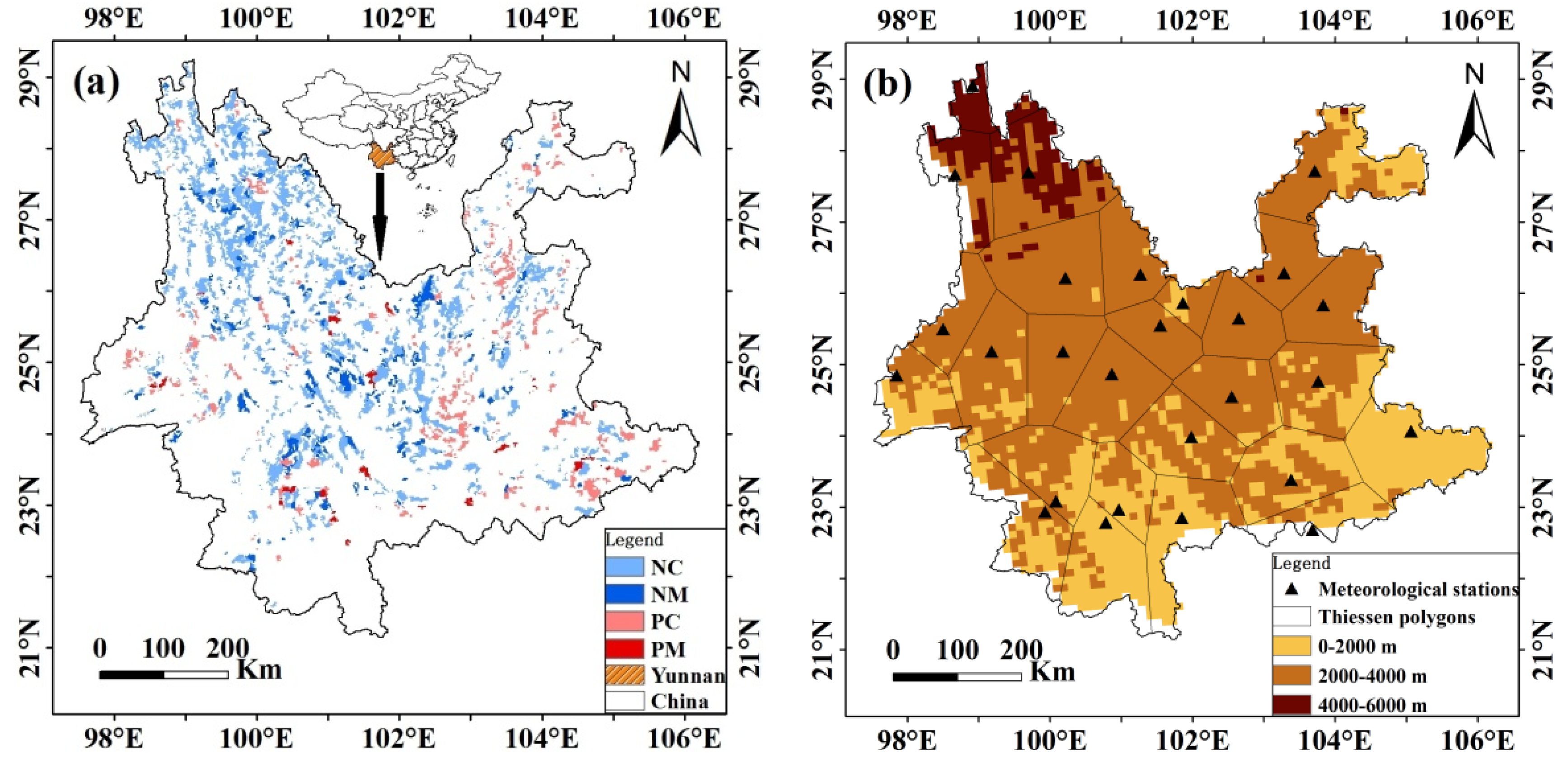
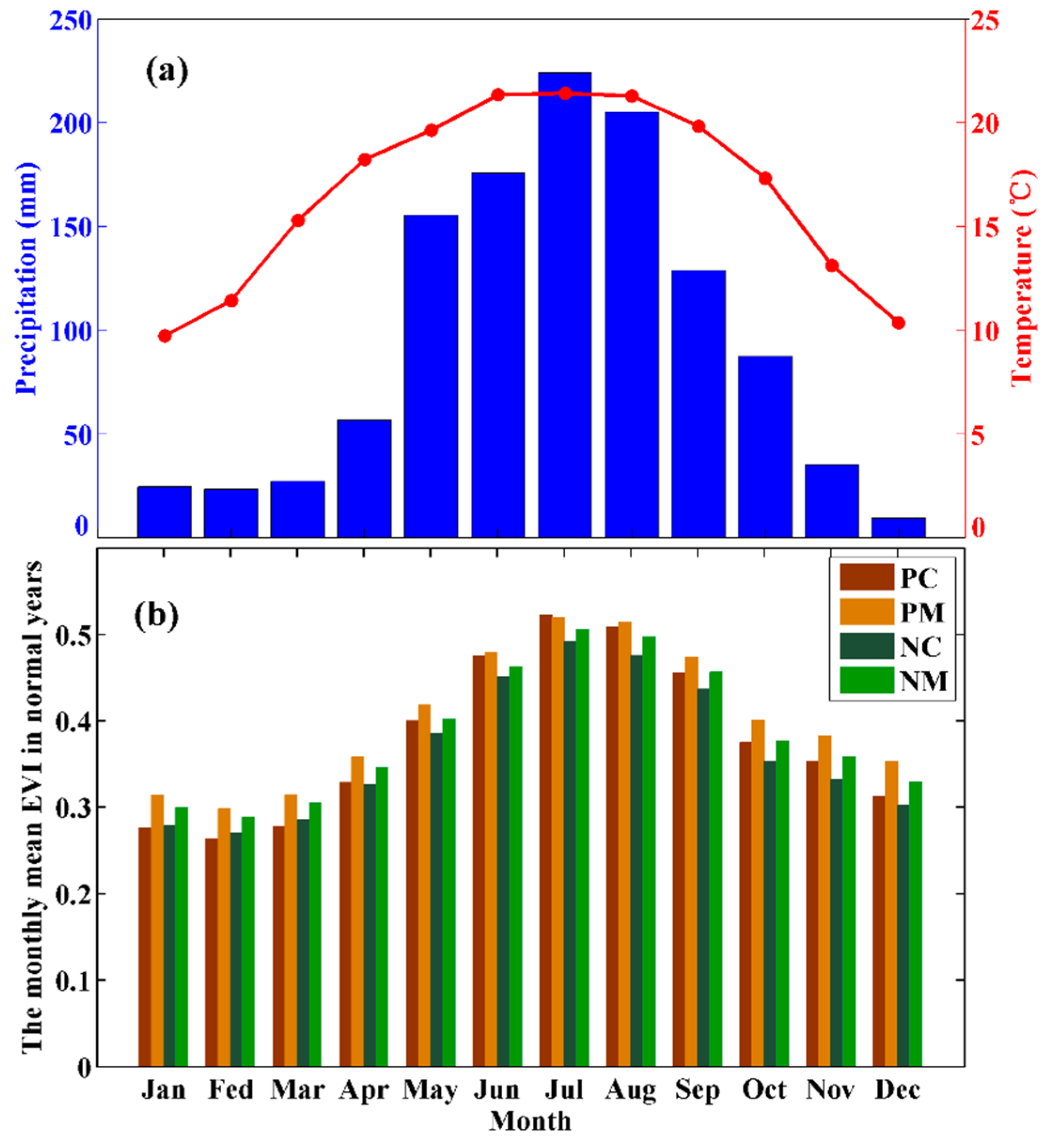
2.1. Study Region

The study region of Yunnan Province is located in southwestern China (97.51°E–106.18°E, 21.13°N–29.25°N) [40], where the altitudes ranges from 592 m to 5808 m (Figure 1a,b). Yunnan primarily has a subtropical monsoon climate, with a mean annual temperature (MAT) of 16.32 °C and mean annual precipitation (MAP) of 1105.12 mm. Higher precipitation and temperatures occur in the summer (June–August) (Figure 2a), and the seasonality of the rainy and dry seasons in Yunnan is related to the Asia monsoon system [44]. According to statistics from China’s Eighth Forest Inventory (2009–2013), forest covers approximately 50.03% of the area of Yunnan Province (Figure S1), where planted and natural forests account for 23.71% and 76.29% [31] (Figure 1a), respectively. The main forest types in Yunnan are broad-leaf mixed forest, Yunnan pine, oak forest, mixed coniferous broad-leaf forest, conifer mixed forest, and other firs [31]. According to the seasonal changes in the forests’ monthly mean EVI in non-drought years, the EVI value changes with the growth of plant leaves (Figure 2b), where the maximum EVI occurs in growing season, especially July and August, for all four forest types and the minimum EVI occurs in the winter (December–March). In recent decades, several drought events with varying intensities and durations have occurred in Yunnan, especially during 2005 and 2009–2014 [32,33], which significantly affected the normal growth of both planted and natural forests. Given the extensive distribution of planted and natural forests as well as the occurrence of drought events, Yunnan Province is an ideal region for studying the responses of forests to drought, and for comparing the potentially different in responses to drought by planted and natural forests, where the overall plan of the study is summarized in Figure 3.

2.2. Materials

2.2.1. MODIS Data

Satellite-derived vegetation indexes such as the NDVI and EVI are attractive for monitoring the dynamics of vegetation at regional and global scales [37,45], which can decrease the multiplicative noise induced by topography [37,46]. This study used MOD13A1 EVI datasets (time resolution of 16 days and spatial resolution of 500 m) from 2001 to 2014, which were obtained from the Land processes distributed active archive center [47], and the ESA was calculated and used as an indicator to characterize the relative changes in forest vitality.

The MODIS EVI imagery data were compiled to match with the forest maps derived from the Eighth Forest Inventory of China. This operation included image mosaicking, spatial resolution conversion (1000 m), and monthly EVI composition based on the maximum value composites method (MVC) [46] using ENVI (5.0) software. To reflect the relative changes in forest vitality and to facilitate comparisons among different forests, the raw EVI data were first transformed into the ESA [38] based on the means and standard deviations of the EVI in non-drought years (Equation (1)). Given that the drought intensity in 2005–2006 was mild [48] and it had little impact on the growth of vegetation in 2007, the non-drought years in this study included 2001–2004 and 2007–2008, when the precipitation was similar to the multi-year average value and there was no apparent water limitation stress on vegetation [32,33]. Therefore, the ESA was used as an indicator to reflect the differences in the EVI for a certain year relative to the long-term mean EVI (2001–2004 and 2007–2008) for the forests:

$$ES{A}_i=\frac{EV{I}_i-Mea{n}_{i-norm}}{S{D}_{i-norm}}$$

(1)

where ESA_i and EVI_i are the EVI standard anomaly and the EVI value for the i-th month (ranging from January to December) for a specific year, respectively, and Mean_i-norm and SD_i-norm correspond to the EVI mean and EVI standard deviation for the i-th month in non-drought years.

2.2.2. Forests’ Inventory Data

Accurately determining the responses to drought by forests depends on the accuracy of the forest map, where the forest map sources employed in previous studies differed. In this study, we employed the forest map derived from the Eighth Forest Inventory (2009–2013) of China (Figure 1a and Figure S1a), which was obtained by remote sensing and a massive forest field survey. The internationally accepted “forest resources continuous inventory method” was used in the survey process, where nearly 20,000 technicians worked on the projects for five years (2009–2013) [49,50]. As a result, this latest forests’ inventory data for China is likely to be most representative. The time span (i.e., 2009–2013) of these maps was similar to our study period (i.e., 2001–2014), which could potentially increase the accuracy of our results. Before performing the spatial analysis, the forest distribution map was first digitized and spatial adjustments were made using ENVI (5.0) and ArcGIS (10.2) (Esri, Environmental Systems Research Institute, New York, NY, USA) image processing software, followed by resampling to a spatial resolution of 1000 m to match with other data, such as the MODIS EVI images, ESA, and the digital elevation models (Figure 1b).

2.2.3. Meteorological Drought Index

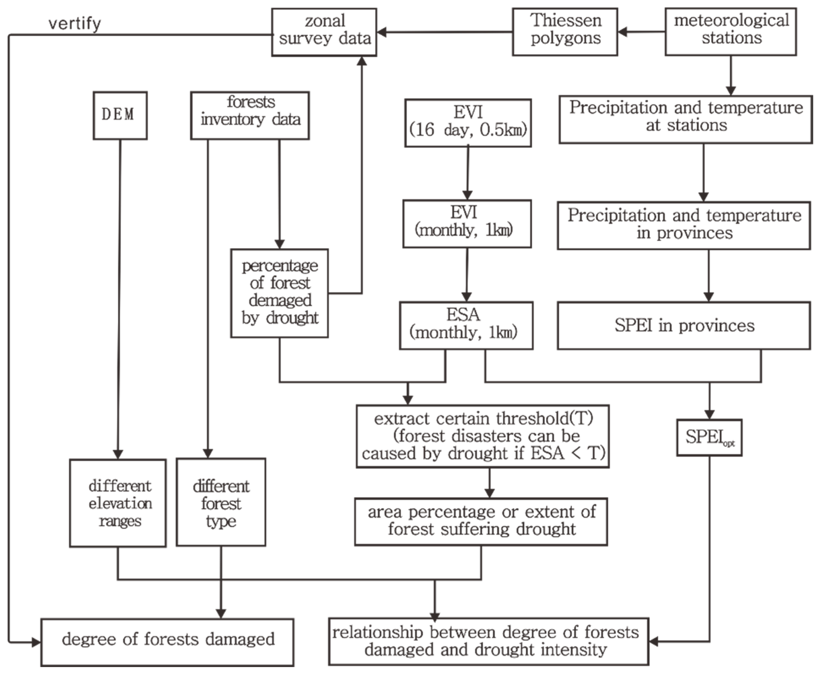
In this study, the SPEI was used to characterize the drought severity. The SPEI calculated using the Penman, Monteith, and Thornthwaite algorithm only differed slightly in Yunnan Province [51], and our previous study showed that the SPEI calculated by Thorthwaite could effectively characterize the drought intensity of Yunnan [43], while previous studies indicated that the impacts of precipitation apparently have a time-lag effect that ranges from several months [43,52,53] to two years [39], so we extended this by half a year (to 30 months) to ensure that it had the optimal time-scale. Thus, the SPEI was calculated according to the following steps [41,42]: (1) the Thornthwaite method was used to calculate the potential evapotranspiration; (2) the cumulative effect of the water surplus and deficit was calculated at specific time scales (1–30 months); (3) the three-parameter log-logistic probability density function was used to fit the cumulative sequence established above; and (4) the cumulative sequence was transformed using the standard normal distribution. This SPEI calculation procedure was derived from DIGITAL.CSIC [54] and it was based on the average monthly precipitation and temperature data for 1960–2014.

The monthly precipitation and temperature data for meteorological sites were obtained from the China meteorological data sharing service system [55] and used to calculate the site-related SPEI. The provincially averaged precipitation and temperature were also calculated based on site observations and used to calculate the averaged SPEI at regional scales. The area weighting method based on Thiessen polygons was employed to calculate the provincial means [56]. First, we produced 27 Thiessen polygons using ArcGIS (10.2) software based on the latitude and longitude of the meteorological site. Second, the areas of the polygons were used as weights to calculate the average monthly precipitation and temperature at the provincial scale.

2.3. Methods

2.3.1. Selecting the Optimal SPEI

The drought intensity derived from the SPEI varies with the month and the time scale employed, so it is necessary to select an optimal SPEI (SPEI_opt) that accurately represents the severity of the drought [41,42]. We calculated the Pearson’s correlation coefficients between the monthly (January to December) ESA (ESA_Jan–Dec) and the corresponding SPEI at 1–30 month time scales (SPEI_1–30) to identify a suitable month and the optimal time scale for the SPEI. Pearson’s correlation coefficient is a method for assessing the strength of the linear relationship between two sets of data (SPSS software, version 20.0) [57]. Thus, we obtained 360 (12 month × 30 time scales) correlation coefficients, which allowed us to determine the suitability of SPEIs at different time scales. Given that the SPEI is a purely meteorological index that contains little vegetation information, the optimal SPEI (SPEI_opt) should have the strongest correlation with the ESA because it reflects relative changes in vegetation under water stress [43].

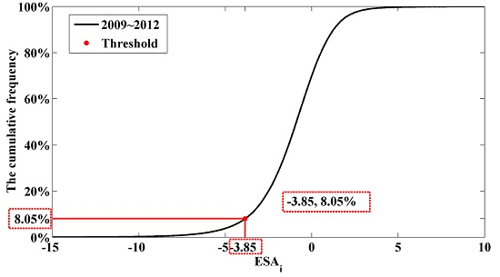
2.3.2. Drought Intensity-Related Indicators

The remote sensing-based ESA is sensitive to the intensity of water stress [58], so we employed it as an indicator to represent the drought response of forests. To distinguish the normal variation in the ESA from the significant decreases in the ESA caused by water limitation stress, we focused our analysis on the forest grids where the ESA was lower than certain thresholds, calculated using Matlab (R2012b).

We defined three thresholds to represent the different responses of planted and natural forests. Two thresholds (T₁ and T₂) were purely statistical, set at −2 and −3 standard deviations (i.e., T₁ = −2 and T₂ = −3). The probability of the ESA in non-drought years being less than two and three standard deviations was quite small, so the change in the forest area and/or proportion with ESA values less than −2 and −3 could represent the extent of forests suffering water stress. The other approximate threshold (T₃) was estimated by the field survey information of severe drought-induced effects on forests (i.e., over 10% of forests area was damaged by the drought [59]). The ESA_i (i ranges from January to December) values reflected the relative changes in forest vitality under water stress whereas the severe drought effects statistics obtained from the field surveys reflected the actual damage to forests, so combining the ESA_i and severe drought effects survey data allowed us to determine the approximate threshold for water stress (T₃, Equation (2)), below which a forest would be damaged to a certain degree. In particular, we used the “cumulative sum” method in the software Matlab (R2012b) to retrieve the threshold based the cumulative ESA_i frequency and the observed forest proportion affected by severe drought effects (Equation (2)).

$$\frac{{\displaystyle \sum A_{i,ES{A}_i\le T_3}}}{{\displaystyle \sum A_i}}=P_d$$

(2)

where $P_d$ is the observed proportion of severe drought effects on forests caused by drought in field surveys; ${\displaystyle \sum A_i}$ and ${\displaystyle \sum A_{i,ES{A}_i\le T_3}}$ are the total forest area for all $ES{A}_i$ grids and the damaged forest area for $ES{A}_i$ less than the threshold $T_3$, respectively; and i ranges from January to December.

To determine P_d and thus T₃, we summarized field survey data obtained from the Chinese State Forestry Administration and the China’s Eighth Forest Inventory (2009–2013, Figure S1), which showed that 8.05% (i.e., P_d) of the forest area in Yunnan Province was affected by the extreme drought during 2009 to 2012 [31,60,61,62,63], and thus the approximate threshold (T₃ = −3.85) that guided by field survey information was retrieved (see Section 3.2).

After obtaining the thresholds (T₁,T₂ and T₃), we determined the spatial distribution of forests where ESA_i was less than these thresholds in each year, which allowed us to summarize the yearly proportion of forest (PT₁, PT₂, and PT₃) that suffered from drought stress (Equation (3), j = 1, 2, 3).

$$P{T}_j=\frac{{\displaystyle \sum A_{i,ES{A}_i\le T_j}}}{{\displaystyle \sum A_i}}$$

(3)

2.3.3. Comparisons between Planted and Natural Forests

To distinguish the potential differences in forest types (i.e., coniferous forests and mixed forests, where the mixed forests represented mixed coniferous broad-leaved forest, which might contain the same forests species as the coniferous planted and natural forests, such as Yunnan pine) and elevation level (i.e., 0–2000, 2000–4000 and 4000–6000 m) for planted and natural forests [19], we divided the forests into six groups based on two forest types and three elevation levels (Figure 1a,b), where each group contained both planted and natural forests. Due to the absence of mixed forest at 4000–6000 m, only five groups were actually analyzed in this study (

Table 1. Groups of planted and natural forests.

Groups	Elevation	Forest Type
Group 1	0–2000 m	Coniferous forest
Group 2	2000–4000 m	Coniferous forest
Group 3	4000–6000 m	Coniferous forest
Group 4	0–2000 m	Mixed forest
Group 5	2000–4000 m	Mixed forest

). Given that the planted and natural forests in each group were similar in terms of the forest type and elevation, we assume that the differences in the ESA reflected the different responses of planted and natural forests. For each group, we used the nonparametric Wilcoxon test to test for significant differences between planted and natural forests, where this method considers information about both the sign of the differences and the magnitude of the differences between pairs (SPSS software, version 20.0) [64].

To distinguish the potential impacts of drought intensity on the different responses of planted and natural forests, we divided the water status into nine groups based on the SPEI hierarchy principle (

Table 2. Scale of drought severity.

Drought Severity	SPEI
Extreme drought	SPEI < −2
Severe drought	−2 < SPEI < −1.5
Moderate drought	−1.5 < SPEI < −1
Mild drought	−1 < SPEI < −0.5
Normal	−0.5 < SPEI < 0.5
Mild wet	0.5 < SPEI < 1
Moderate wet	1 < SPEI < 1.5
Severe wet	1.5 < SPEI < 2
Extreme wet	SPEI > 2

) [48]. Given that the PT₃ was based on the approximate T₃ threshold which was estimated by field survey information, the PT₃ indicator was to investigate the relationship between drought intensity (SPEI_opt) and changes in forest vitality (ESA_i) using nonlinear regression. We then compared the differences in sensitivity to drought for each class for the planted and natural forests. Considering the limitations of meteorological data from different elevation ranges and forests, where significant errors would be caused by interpolating the SPEI, the provincial SPEI was used for each forest group.

To remove the potential effects of regional variations in drought, we compared the different proportions of planted and natural forests with the same drought stresses in all drought years using the nonparametric Wilcoxon test. First, to unify the drought conditions for the pairs of proportion data for planted and natural forests, we produced Thiessen polygons (N = 27) based on the latitude and longitude of the meteorological sites (Figure 1b), where each polygon corresponded to a single meteorological site, so similar climate conditions were characterized by the SPEI of the sites. Next, all of the polygons affected by a certain drought stress (i.e., SPEI less than −0.5) in all drought years (N = 8, 2005–2006 and 2009–2014) were selected based on the scale of drought severity (Table 2) [48]. There were only 15 polygons for mixed forests with both planted and natural forests, so only 127/70 pairs of proportion data were compared using the nonparametric Wilcoxon test (SPSS software, 20.0) for the coniferous/mixed forests group. In addition, we calculated the differences in the proportions of planted and natural forests (D) in these polygons with drought stress, and a pie chart was used to show the sign and the magnitude of all the D values based on each polygon, where the percentage in the chart increased with the value of D. In addition, the minus (−) and plus (+) signs of D were denoted as red and grey, respectively. Note that all abbreviations used in this study are summarized in the

Table 3. Definitions of the abbreviation used in this study.

The Abbreviation	Definition
ESA	EVI standard anomaly.
T1, T2, T3	Thresholds of −2, −3, and −3.85.
PT1, PT2, PT3	Yearly proportions of ESA less than the thresholds of −2, −3, and −3.85, respectively.
PC, PM, NC, NM	Planted coniferous forests, planted mixed forests, natural coniferous forests and natural mixed forests, respectively.
D, DC, DM	Difference between planted and natural forests in PT3, difference between planted coniferous forests and natural coniferous forests, and difference between planted mixed forests and natural mixed forests, respectively.

.

3. Results

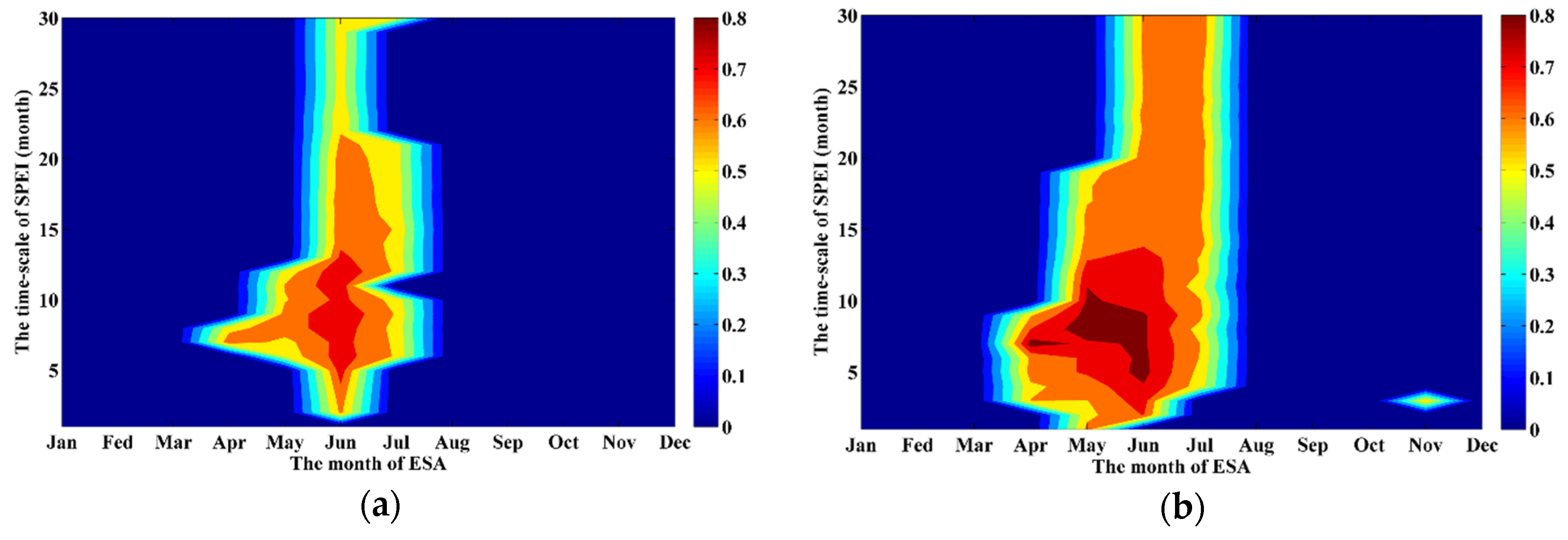
3.1. Optimal SPEI for the Planted and Natural Forests

The correlations between the ESAs from January to December (ESA_Jan–Dec) and the SPEIs with time scales of 1–30 months (SPEI_1–30) are shown in Figure 4. These results indicated that the relationship between the ESA and SPEI was time scale-dependent, and thus selecting a suitable time scale for SPEI was crucial when using it as an indicator of drought intensity. The results also indicated that although there were some slight differences among different forests, the patterns in the correlation coefficients were quite similar (Figure 4a,b; Figure S2a,b).

Both the planted and natural mixed forests exhibited strong covariation between the ESA in June (ESA_Jun) and the SPEI over a five-month time scale (SPEI_Jun,5), with correlation coefficients of 0.868 and 0.825, respectively (Figure S2a,b). Thus, SPEI_Jun,5 was most suitable for characterizing the effects of physiological drought stress on both planted and natural mixed forests. The strongest correlation between ESA and SPEI in planted coniferous forests was found for the ESA in June (ESA_Jun) and the SPEI over 5–9-month time scales (Figure 4a). Similarly, for the natural coniferous forests, the strongest correlations were found for the ESA from April to June and the SPEI over 5–8-month time scales (Figure 4b).

Given that the SPEI in June and a time scale of five months (SPEI_Jun,5) was the optimal indicator for physiological drought stress in all planted and natural forests, we selected the SPEI_Jun,5 to characterize the drought intensity for all forests. Thus, the June ESA (ESA_Jun) was used to characterize the relative changes in forest vitality.

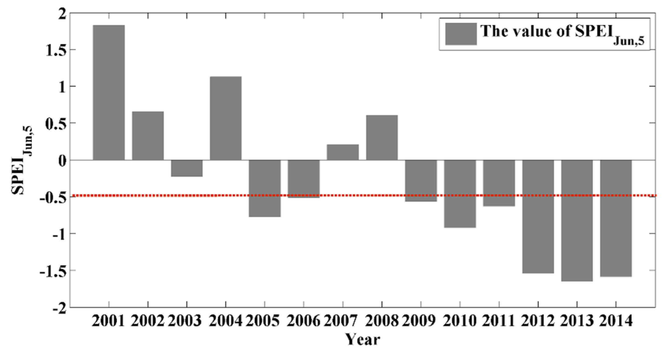
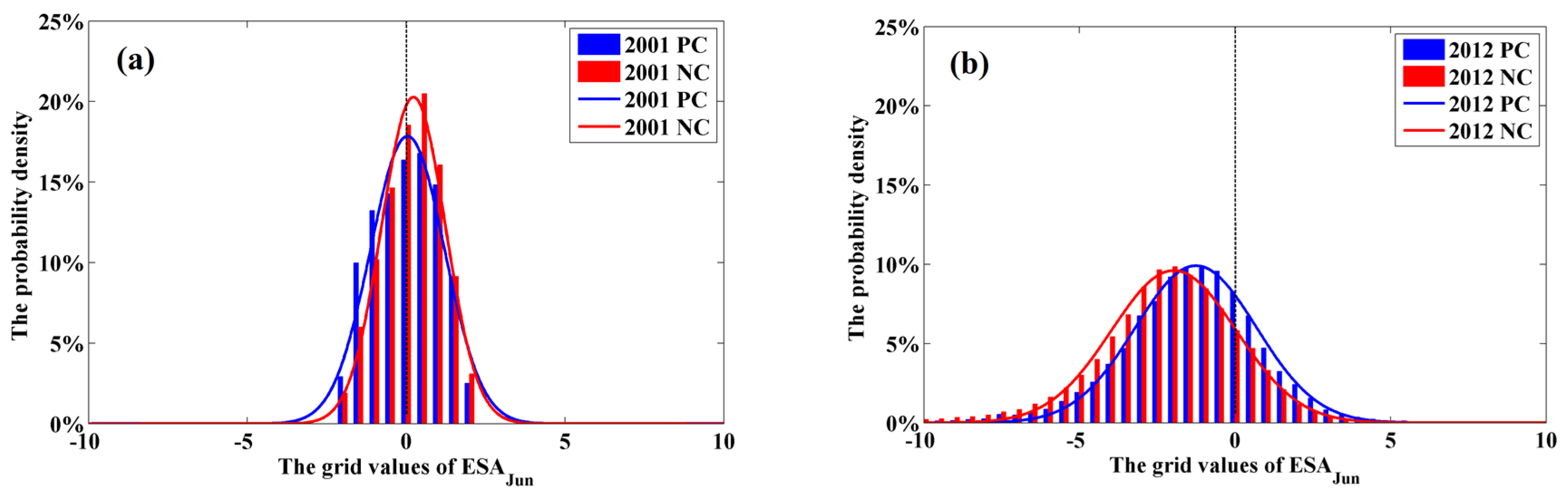
3.2. Potential Impacts of Drought on Forests

The time trends in the SPEI_Jun,5 (Figure 5) showed that the water status was adequate in the non-drought years (i.e., 2001–2004 and 2007–2008), with SPEI_Jun,5 values in normal ranges (Table 2). However, in the drought years (i.e., 2005–2006 and 2009–2014), the precipitation was lower than that in the non-drought years and the SPEI_Jun,5 values were lower than those in the non-drought years. In addition, 2001 was a representative non-drought year and 2012 was not only the extreme drought year, but it corresponded to the last period of forest survey data (2009–2012), thus, we focused on the vitality of forests in 2001 and 2012.

The remote sensing-based ESA_Jun can characterize the relative changes in forest vitality, so the ESA_Jun was combined with the field survey-based statistical data for the damaged forest area caused by drought to obtain the approximate threshold of T₃ (i.e., T₃ = −3.85) (Figure 6).

The results indicated that the drought in 2012 had extensive impacts on the ESA_Jun for forests in Yunnan Province (Figure S3). As expected, using lower standard deviation thresholds (i.e., ESA_Jun < T₁ or ESA_Jun < T₂) would apparently overestimate the number of forests that experienced a severe drought effects (Figure S3b–d).

To distinguish the potential impacts and possible differences in the effects of drought stress on planted and natural forests, we compared their probability distributions in terms of the ESA_Jun in 2001 and 2012 (Figure 7 and Figure S4). The results indicated that when the water stress was absent, the PC-NC and PM-NM had similar probability distributions (Figure 7a and Figure S4a). However, in the extreme drought year, the ESAs were significantly lower for both the planted and natural forests (Figure 7b and Figure S4b), which showed that the relative vitality of both planted and natural forests was sensitive to water stress. Further analysis indicated that the ESAs in natural forests (NC, NM) exhibited higher decreases compared with those in the planted forests (PC, PM) (Figure 7b and Figure S4b), which indicated that the natural forests are probably more vulnerable than planted forests when subjected to similar water stress caused by extreme drought events.

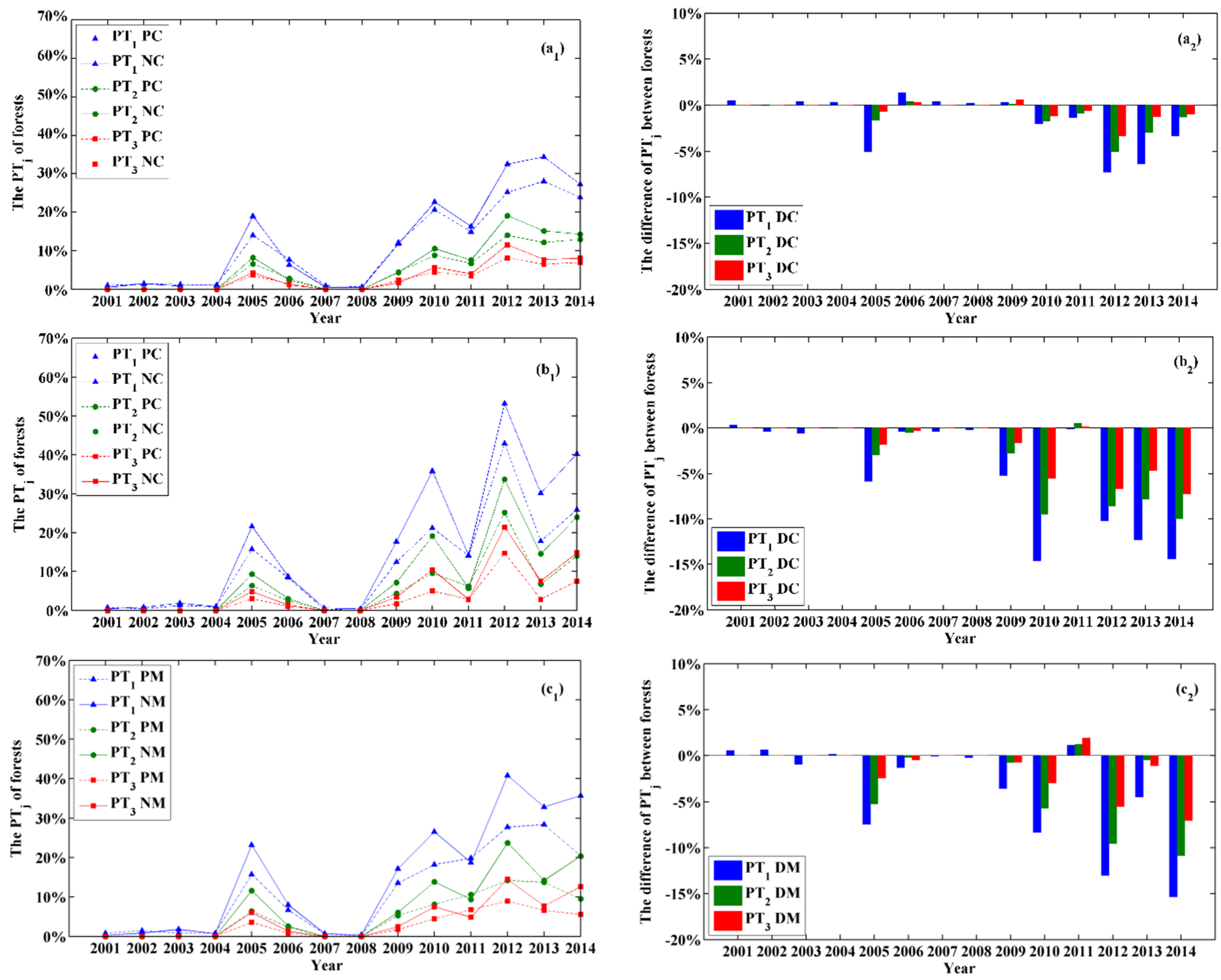
3.3. Comparisons of the Drought Responses by Planted and Natural Forests

The results indicated that the drought responses differed between the planted and natural forests, where the responses were related to the forest type (Figure 8 and Figure S5). In particular, the differences in PT_j (j =1, 2, 3) for Group 1 (coniferous forest at 0–2000 m), Group 2 (coniferous forest at 2000–4000 m), and Group 4 (mixed forest at 0–2000 m) were greater than those between the other two groups (i.e., Groups 3 and 5), which did not differ. The difference determined according to the T₁ and T₂ threshold (i.e., PT₁ and PT₂) was higher than that based on the T₃ threshold (i.e., PT₃) (Figure 8, Figure S5a₂ and Figure S5b₂). These results suggest that natural forests were more vulnerable than planted forests under similar drought intensities.

The results confirmed that the differences in the PT₃ determined by T₃ were significant (p < 0.05) for Groups 1, 2, and 4, which were consistent with those based on PT₂ (T₂), but the differences in the PT₁ (T₁) were also significant according to the Wilcoxon tests for Group 2 and Group 4.

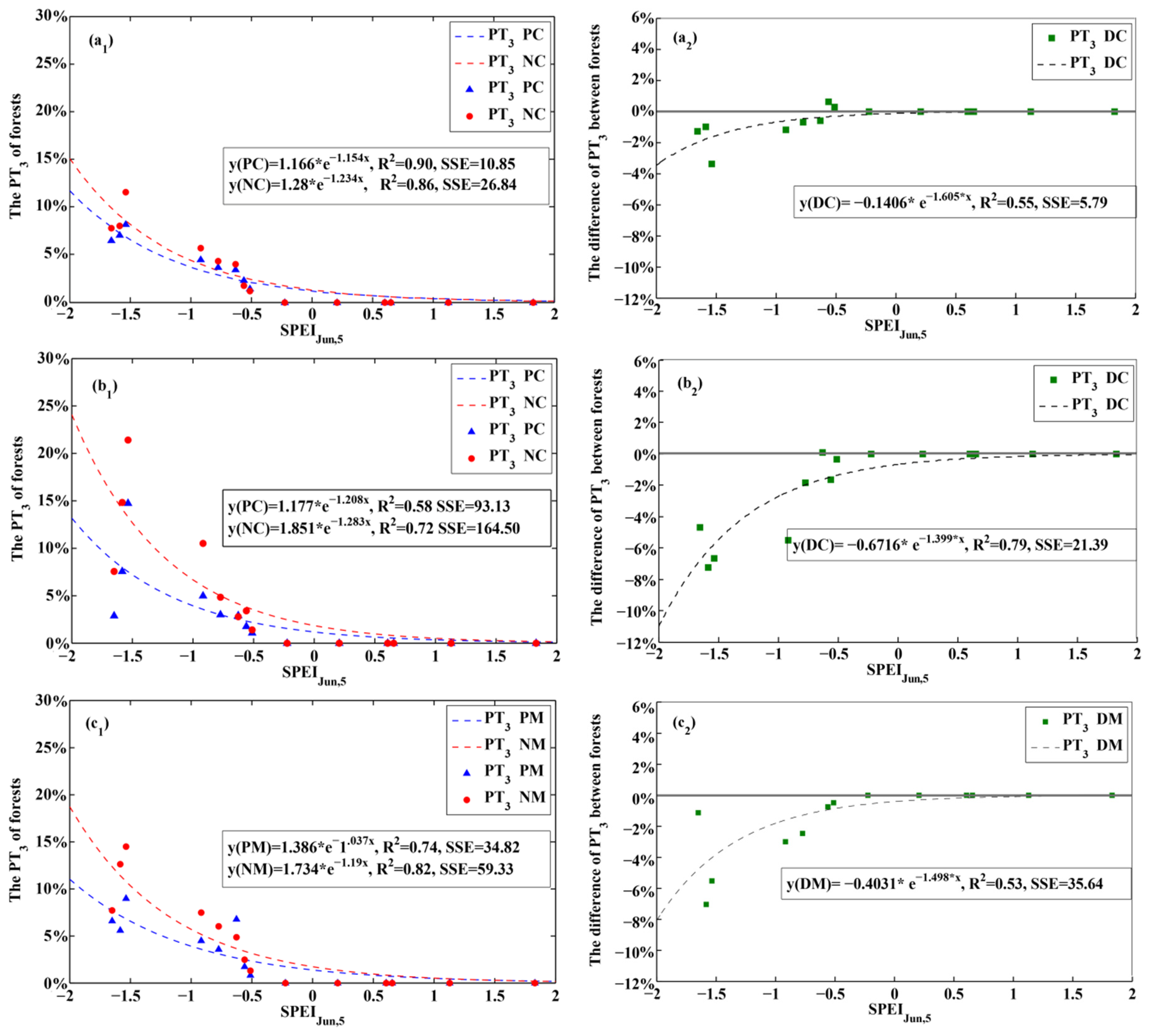
3.4. Responses of Planted and Natural Forests to Drought Intensity

The results (Figure 9a_1, b₁ and c₁; Figure S6a₁,b₁) showed that the PT₃ increased exponentially for all five forest groups as SPEI_Jun,5 decreased (i.e., increased water stress intensity), thereby indicating that the proportion of damaged forests increased rapidly as the drought intensity increases.

The relationships between PT₃ and SPEI_Jun,5 were similar for both planted and natural forests in the five forest groups, but comparisons of the sensitivity to drought intensity indicated that there were apparent differences among groups (Figure 9a₂,b₂ and c₂, and Figure S6a₂, b₂). The results showed that the differences in the relationships fitted between PT₃ and SPEI_Jun,5 for the planted and natural forests were quite similar in Group 3 (coniferous forests at 4000–6000 m) and Group 5 (mixed forests at 2000–4000 m), and the differences in PT₃ were random around zero (Figure S6a₁ and b₁). These results were consistent with the results obtained from the nonparametric Wilcoxon tests (

Table 4. Results of nonparametric Wilcoxon tests for 2001–2014.

Group	N	ESAJun < T1				ESAJun < T2				ESAJun < T3
		N-n	N-p	N-e	P1	N-n	N-p	N-e	P2	N-n	N-p	N-e	P3
Group 1	14	7	7	0	0.272	2	6	6	0.036	2	6	6	0.050
Group 2	14	1	13	0	0.022	1	7	6	0.025	1	7	6	0.017
Group 3	14	9	5	0	0.975	4	4	6	0.779	4	4	6	1.000
Group 4	14	4	10	0	0.030	1	7	6	0.05	1	7	6	0.050
Group 5	14	7	7	0	0.510	6	2	6	0.327	6	2	6	0.484

Note: p-values < 0.05 indicate significant differences according to the nonparametric Wilcoxon test. N-n, N-p, and N-e indicate that the differences in PT between planted and natural forests were negative, positive, and equal, respectively. The P₁, P₂, and P₃ are the significant values for “ESA_Jun < T₁”, “ESA_Jun < T₂”, and “ESA_Jun < T₃”, respectively.

), which indicated that there were no significant differences in the planted and natural forests in these two groups. For the other three groups, the results indicated that although PT₃ decreased exponentially as SPEI_Jun,5 increased in both the planted and natural forests (Figure 9a₁, b₁ and c₁), the natural forests exhibited greater sensitivity to changes in the drought intensity compared with the planted forests. In particular, under higher drought intensities, the differences in PT₃ between the planted and natural forests tended to increase with the water stress intensity (Figure 9a₂, b₂ and c₂).

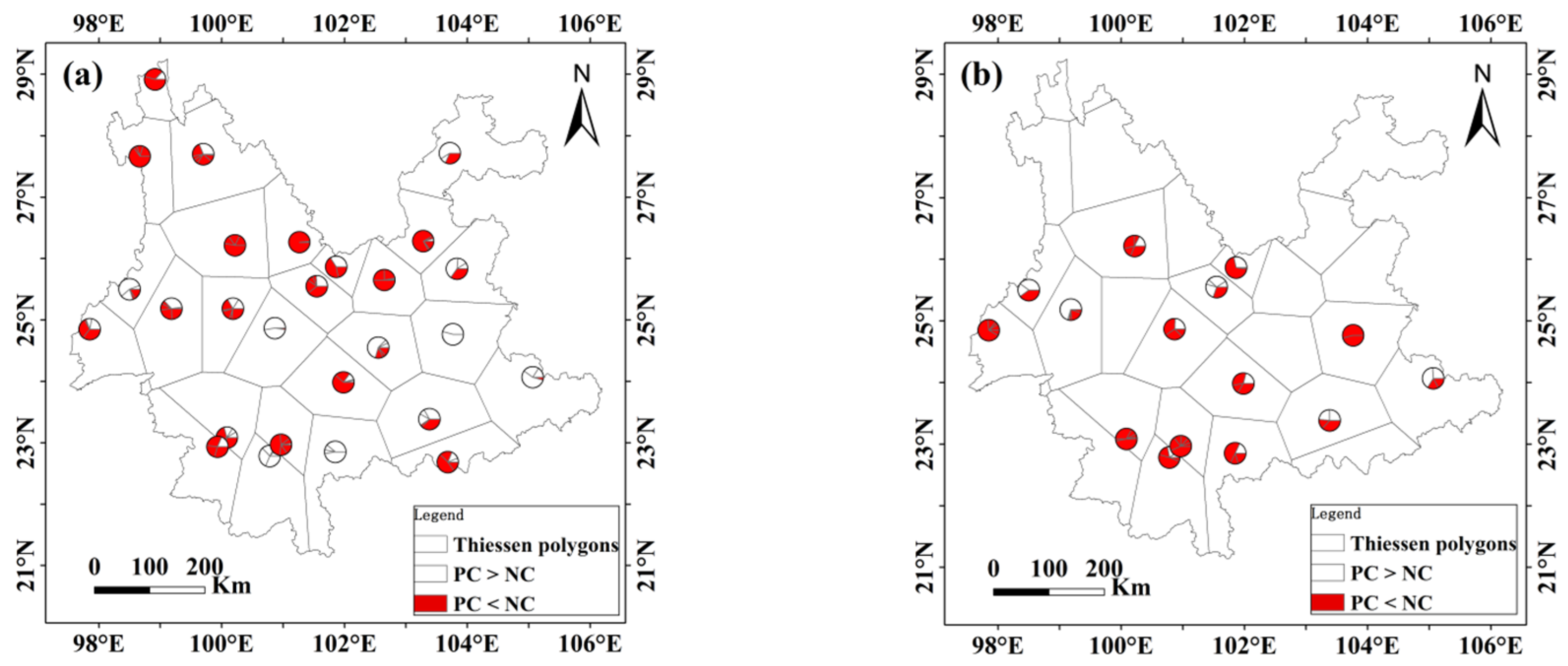
3.5. Application of the ForestApproximate Threshold in Small Regions

The results of the nonparametric Wilcoxon tests (

Table 5. Nonparametric Wilcoxon tests for drought years.

Forests Group	N	N-n (Percentage, Sum of Rank)	N-p (Percentage, Sum of Rank)	N-e (Percentage)	p
Coniferous	127	55 (43.31%, 3235.00)	72 (56.69%, 4893.00)	0 (0%)	0.046 **
Mixed	70	25 (35.71%, 814.50)	41 (58.57%, 1396.50)	4 (5.72%)	0.063 *

N-n, N-p, and N-e indicate that the difference in PT₃ (D) between planted and natural forests was negative, positive, and equal, respectively. ** Significantly different at p < 0.05; * significantly different at p < 0.1. The “sum of rank” is the sum of the ranks for N-n and N-p.

) showed that PT₃ was greater for natural forests (NC, NM) than planted forests (PC, PM) in drought conditions, and the differences in the coniferous and mixed forest groups were significant at p < 0.05 and p < 0.1, respectively. In addition, the 56.69% and 58.57% of the polygons in Figure 10a,b showed that the amount of damage in natural forests was more severe than that in planted forests under the same drought conditions. Thus, the results determined at the polygon scale were consistent with those at the provincial scale, where both showed that natural forests were more vulnerable than planted forests.

4. Discussion

4.1. Ecological Significance of the Optimal SPEI

The SPEI meteorological drought index has been used widely to characterize the severity of drought [65,66]. However, the SPEI is a pure meteorological index, which contains little information about vegetation and its value also varies with the time scale selected, so the accuracy of drought assessments based on the SPEI depends on the suitability of the time scale selected [39,43]. In this study, we combined the remote sensed ESA and SPEI information over different time scales to determine the optimal SPEI, and we found that the most suitable month and optimal time scale for the SPEI was SPEI_Jun,5. This is because the forest vitality in June required a relatively high amount of water to satisfy the rapid growth demands, while the previous precipitation was relatively lower, so the forests were sensitive to the water conditions in June as well as the previous cumulative effect of the water balance (i.e., February to June). Given the time-lag effect of the vegetation response to moisture [53], the vegetation in Yunnan Province exhibited high sensitivity to the SPEI for June. In addition, many studies have shown that the growth of forests in the summer (June, July, and August) is sensitive to the water conditions in the previous and current month [39,43,67], so the growth state of forests in the summer has always been used as an indicator to monitor the response of forests to drought [39,43]. Thus, using the June ESA as the optimal indicator may be applicable to other studies.

4.2. Differences between Planted and Natural Forests

Compared with natural forests, planted forests have received more human management, such as human selection (site, species and planting density), plowing, and the use of fertilizers and herbicides [16], as well as being located in relatively moist environment [18] with more irrigation, so the sensitivity of planted forests to water deficits will be reduced [17]. However, human management which aims to maximize the economic income of forests may potentially undermine the biodiversity [68] and weaken the forest resilience [69,70]. In the long-term, the relaxation of human management would potentially increase the diversity of planted forests and then enhance the forest resilience. In addition, planted forests started with the development of GCP program of Yunnan Province during the early 2000s, which implies that the planted forests are relatively younger than natural forests. As a result, the forest age effect is another factor need to be considered as many studies found that forest age affects the response of forests to drought [71,72,73]. For example, Linares et al. found that older forests are more sensitive to temperature than younger forests [71], due to a difference in canopy temperature and thus vapor pressure deficit given that canopies of old trees are usually exposed to more light than canopies of young trees [74]. The less resistibility of older forests than that of young ones to drought may due to the vulnerability of old forests to xylem cavitation [75], and the increased size and structural complexity could augment maintenance respiration costs and reduce the efficiency of the hydraulic pathway [71].

4.3. Potential Effects of Different Spatial Scales

Compared with the province scale, the Thiessen polygons derived from meteorological stations could reflect more detailed geographical differences, thereby possibly eliminating some potential influences caused by spatial heterogeneities [76], e.g., every polygon having similar drought conditions. In this study, we found that the results obtained were consistent, where the natural forests were more vulnerable than the planted forests at both the provincial and Thiessen polygon scales. According to the results obtained at the polygon scale, a small number of polygons showed that planted forests were more vulnerable than natural forests, possibly due to the differences in the levels of forest management, regional water sources, or other factors [8,17,77,78]. However, most of the polygons showed that natural forests were more vulnerable to drought than the planted forests, so the result was reasonable.

4.4. Limitations and Prospects

There were still some uncertainties in this study due to limitations on the information available. For example, some errors may have occurred during the matching process between the forest distribution map and remote sensing images, as well as in the spatial resolution resampling process. In addition, there may have been some uncertainty because the spatial distribution of forest damage was not available and a large scale field survey would be too expensive in terms of both labor and finance. However, given that more severely damaged forests usually exhibit higher decreases in the EVI, the statistical information for damaged forest (i.e., damage ratio) could be used as an indicator to identify the most likely locations when the ESA is processed. Furthermore, there were limitations on the spatial distribution of the drought intensity and when we interpolated these site-derived SPEIs to spatial grids and matched them with the remote sensed EVI, the errors and uncertainties caused by interpolation were unavoidable, so the provincial SPEI_Jun was used for every elevation range and forest type, which probably still caused some errors. Thus, to further avoid the regional differences in droughts, the results at the provincial scale were verified based on the results using Thiessen polygons for the same drought events, which demonstrated that the results were consistent at the two scales, i.e., natural forests were more vulnerable to drought than planted forests.

Forests’ inventory data and remote sensing data were both used in this study to compare the different responses of planted and natural forests, where we obtained the matching point (ESA_Jun = −3.85) of forests, which accounted for the same proportion of forest declines, and we finally showed that natural forests were more vulnerable to drought than planted forests. However, in the current study, it was difficult to determine the differences in resilience between the forests, which would require more comprehensive datasets to make resilience comparison at the spatial-grid scale [79,80].

5. Conclusions

It is important to understand the different responses of planted and natural forests to drought because this may form the basis of forest risk assessments and management in the context of the predicted increases in extreme drought events in the future. In this study, we combined multiple types of data obtained from meteorological observations, remote sensing (MODIS13A1), and the forests map of the China’s Eighth Forest Inventory across Yunnan Province to compare the response characteristics of planted and natural forests to different drought intensities. The results indicated that the SPEI in June and over a time scale of five months (SPEI_Jun,5) was most effective for characterizing the water stress for forests in Yunnan Province, which had the strongest correlation with the ESA_Jun. All of the forests in Yunnan were affected by drought events, but their responses varied according to the forest type, elevation and drought intensity. In general, natural forests were more sensitive and vulnerable to drought than planted forests. The forests’ inventory survey revealed that 8.05% of forests were affected by drought, which corresponded an approximate threshold of −3.85 (i.e., ESA_Jun= −3.85), below which (i.e., ESA_Jun < −3.85) severe drought-induced effects on forests could occur. Given that extreme drought events are predicted to increase in the future, natural forests may require greater management because they are more sensitive and vulnerable to drought.

References

1. Foster, P. The potential negative impacts of global climate change on tropical montane cloud forests. Earth Sci. Rev. 2001, 55, 73–106. [Google Scholar] [CrossRef]
2. Dai, A.; Trenberth, K.E.; Qian, T.T. A global dataset of palmer drought severity index for 1870–2002: Relationship with soil moisture and effects of surface warming. J. Hydrometeorol. 2004, 5, 1117–1130. [Google Scholar] [CrossRef]
3. Dale, V.H.; Joyce, L.A.; McNulty, S.; Neilson, R.P. The interplay between climate change, forests, and disturbances. Sci. Total Environ. 2000, 262, 201–204. [Google Scholar] [CrossRef]
4. Choat, B.; Jansen, S.; Brodribb, T.J.; Cochard, H.; Delzon, S.; Bhaskar, R.; Bucci, S.J.; Feild, T.S.; Gleason, S.M.; Hacke, U.G.; et al. Global convergence in the vulnerability of forests to drought. Nature 2012, 491, 752–755. [Google Scholar] [CrossRef] [PubMed]
5. Allen, C.D.; Macalady, A.K.; Chenchouni, H.; Bachelet, D.; McDowell, N.; Vennetier, M.; Kitzberger, T.; Rigling, A.; Breshears, D.D.; Hogg, E.H.; et al. A global overview of drought and heat-induced tree mortality reveals emerging climate change risks for forests. For. Ecol. Manag. 2010, 259, 660–684. [Google Scholar] [CrossRef]
6. Field, C.B.; Barros, V.; Stocker, T.F.; Dahe, Q.; Dokken, D.J.; Ebi, K.L.; Mastrandrea, M.D.; Mach, K.J.; Plattner, G.K.; Allen, S.K.; et al. Managing the Risks of Extreme Events and Disasters to Advance Climate Change Adaptation; A Special Report of Working Groups I and II of the Intergovernmental Panel on Climate Change: Cambridge, UK, 2012; p. 582. [Google Scholar]
7. Bertrand, R.; Lenoir, J.; Piedallu, C.; Riofrio-Dillon, G.; de Ruffray, P.; Vidal, C.; Pierrat, J.-C.; Gegout, J.-C. Changes in plant community composition lag behind climate warming in lowland forests. Nature 2011, 479, 517–520. [Google Scholar] [CrossRef] [PubMed]
8. Pawson, S.M.; Brin, A.; Brockerhoff, E.G.; Lamb, D.; Payn, T.W.; Paquette, A.; Parrotta, J.A. Plantation forests, climate change and biodiversity. Biodivers. Conserv. 2013, 22, 1203–1227. [Google Scholar] [CrossRef]
9. Klein, T.; Yakir, D.; Buchmann, N.; Gruenzweig, J.M. Towards an advanced assessment of the hydrological vulnerability of forests to climate change-induced drought. New Phytol. 2014, 201, 712–716. [Google Scholar] [CrossRef] [PubMed]
10. McDowell, N.G.; Fisher, R.A.; Xu, C.; Domec, J.C.; Holtta, T.; Mackay, D.S.; Sperry, J.S.; Boutz, A.; Dickman, L.; Gehres, N.; et al. Evaluating theories of drought-induced vegetation mortality using a multimodel-experiment framework. New Phytol. 2013, 200, 304–321. [Google Scholar] [CrossRef] [PubMed]
11. Sperry, J.S.; Hacke, U.G.; Oren, R.; Comstock, J.P. Water deficits and hydraulic limits to leaf water supply. Plant Cell Environ. 2002, 25, 251–263. [Google Scholar] [CrossRef] [PubMed]
12. Huntingford, C.; Cox, P.M.; Lenton, T.M. Contrasting responses of a simple terrestrial ecosystem model to global change. Ecol. Model. 2000, 134, 41–58. [Google Scholar] [CrossRef]
13. Brodribb, T.J.; Cochard, H. Hydraulic failure defines the recovery and point of death in water-stressed conifers. Plant Physiol. 2009, 149, 575–584. [Google Scholar] [CrossRef] [PubMed]
14. Meason, D.F.; Mason, W.L. Evaluating the deployment of alternative species in planted conifer forests as a means of adaptation to climate change-case studies in new zealand and scotland. Ann. For. Sci. 2014, 71, 239–253. [Google Scholar] [CrossRef]
15. Bremer, L.L.; Farley, K.A. Does plantation forestry restore biodiversity or create green deserts? A synthesis of the effects of land-use transitions on plant species richness. Biodivers. Conserv. 2010, 19, 3893–3915. [Google Scholar] [CrossRef]
16. Brockerhoff, E.G.; Jactel, H.; Parrotta, J.A.; Quine, C.P.; Sayer, J. Plantation forests and biodiversity: Oxymoron or opportunity? Biodivers. Conserv. 2008, 17, 925–951. [Google Scholar] [CrossRef]
17. Zhou, J.; Zhang, Z.; Sun, G.; Fang, X.; Zha, T.; McNulty, S.; Chen, J.; Jin, Y.; Noormets, A. Response of ecosystem carbon fluxes to drought events in a poplar plantation in northern china. For. Ecol. Manag. 2013, 300, 33–42. [Google Scholar] [CrossRef]
18. Guo, Q.; Ren, H. Productivity as related to diversity and age in planted versus natural forests. Glob. Ecol. Biogeogr. 2014, 23, 1461–1471. [Google Scholar] [CrossRef]
19. Sloan, S.; Sayer, J.A. Forest resources assessment of 2015 shows positive global trends but forest loss and degradation persist in poor tropical countries. For. Ecol. Manag. 2015, 352, 134–145. [Google Scholar] [CrossRef]
20. Fashing, P.J.; Nga, N.; Luteshi, P.; Opondo, W.; Cash, J.F.; Cords, M. Evaluating the suitability of planted forests for african forest monkeys: A case study from kakamega forest, kenya. Am. J. Primatol. 2012, 74, 77–90. [Google Scholar] [CrossRef] [PubMed]
21. Domec, J.-C.; King, J.S.; Ward, E.; Christopher Oishi, A.; Palmroth, S.; Radecki, A.; Bell, D.M.; Miao, G.; Gavazzi, M.; Johnson, D.M.; et al. Conversion of natural forests to managed forest plantations decreases tree resistance to prolonged droughts. For. Ecol. Manag. 2015, 355, 58–71. [Google Scholar] [CrossRef]
22. Broeckx, L.S.; Verlinden, M.S.; Berhongaray, G.; Zona, D.; Fichot, R.; Ceulemans, R. The effect of a dry spring on seasonal carbon allocation and vegetation dynamics in a poplar bioenergy plantation. GCB Bioenergy 2014, 6, 473–487. [Google Scholar] [CrossRef]
23. Sánchez-Salguero, R.; Camarero, J.J.; Dobbertin, M.; Fernández-Cancio, Á.; Vilà-Cabrera, A.; Manzanedo, R.D.; Zavala, M.A.; Navarro-Cerrillo, R.M. Contrasting vulnerability and resilience to drought-induced decline of densely planted vs. Natural rear-edge pinus nigra forests. For. Ecol. Manag. 2013, 310, 956–967. [Google Scholar] [CrossRef]
24. Li, S.; Luo, Y.-Q.; Wu, J.; Zong, S.-X.; Yao, G.-L.; Li, Y.; Liu, Y.-M.; Zhang, Y.-R. Community structure and biodiversity in plantations and natural forests of seabuckthorn in southern Ningxia, China. For. Stud. China 2009, 11, 49–54. [Google Scholar]
25. Fernández, M.E.; Gyenge, J.; Schlichter, T. Water flux and canopy conductance of natural versus planted forests in Patagonia, south America. Trees 2008, 23, 415–427. [Google Scholar] [CrossRef]
26. Wang, L.; Zhang, Y.; Berninger, F.; Duan, B. Net primary production of chinese fir plantation ecosystems and its relationship to climate. Biogeosciences 2014, 11, 5595–5606. [Google Scholar] [CrossRef]
27. Samanta, A.; Ganguly, S.; Hashimoto, H.; Devadiga, S.; Vermote, E.; Knyazikhin, Y.; Nemani, R.R.; Myneni, R.B. Amazon forests did not green-up during the 2005 drought. Geophys. Res. Lett. 2010, 37. [Google Scholar] [CrossRef]
28. Zhang, Y.; Peng, C.; Li, W.; Fang, X.; Zhang, T.; Zhu, Q.; Chen, H.; Zhao, P. Monitoring and estimating drought-induced impacts on forest structure, growth, function, and ecosystem services using remote-sensing data: Recent progress and future challenges. Environ. Rev. 2013, 21, 103–115. [Google Scholar] [CrossRef]
29. Xiao, J. Satellite evidence for significant biophysical consequences of the “grain for green” program on the loess plateau in china. J. Geophys. Res. Biogeosci. 2014, 119, 2261–2275. [Google Scholar] [CrossRef]
30. Chen, X.; Zhang, X.; Zhang, Y.; Wan, C. Carbon sequestration potential of the stands under the grain for green program in yunnan province, china. For. Ecol. Manag. 2009, 258, 199–206. [Google Scholar] [CrossRef]
31. State Forestry Administration of the People’s Republic of China. The Main Results at Eighth National Forest Resources Inventory (2009–2013). 2015. Available online: http://www.forestry.gov.cn/main/65/content-659670.html (accessed on 8 October 2014). [Google Scholar]
32. Yang, J.; Gong, D.; Wang, W.; Hu, M.; Mao, R. Extreme drought event of 2009/2010 over Southwestern China. Meteorol. Atmos. Phys. 2012, 115, 173–184. [Google Scholar] [CrossRef]
33. Zhao, X.; Wei, H.; Liang, S.; Zhou, T.; He, B.; Tang, B.; Wu, D. Responses of natural vegetation to different stages of extreme drought during 2009–2010 in Southwestern China. Remote Sens. 2015, 7, 14039–14054. [Google Scholar] [CrossRef]
34. Vincent, G.; de Foresta, H.; Mulia, R. Co-Occurring tree species show contrasting sensitivity to enso-related droughts in planted dipterocarp forests. For. Ecol. Manag. 2009, 258, 1316–1322. [Google Scholar] [CrossRef]
35. Gustafson, E.J.; Sturtevant, B.R. Modeling forest mortality caused by drought stress: Implications for climate change. Ecosystems 2013, 16, 60–74. [Google Scholar] [CrossRef]
36. Xie, Y.; Wang, X.; Silander, J.A., Jr. Deciduous forest responses to temperature, precipitation, and drought imply complex climate change impacts. Proc. Natl. Acad. Sci. USA 2015, 112, 13585–13590. [Google Scholar] [CrossRef] [PubMed]
37. Huete, A.; Didan, K.; Miura, T.; Rodriguez, E.P.; Gao, X.; Ferreira, L.G. Overview of the radiometric and biophysical performance of the modis vegetation indices. Remote Sens. Environ. 2002, 83, 195–213. [Google Scholar] [CrossRef]
38. Maeda, E.E.; Heiskanen, J.; Aragao, L.E.O.C.; Rinne, J. Can MODIS EVI monitor ecosystem productivity in the amazon rainforest? Geophys. Res. Lett. 2014, 41, 7176–7183. [Google Scholar] [CrossRef]
39. Huang, K.; Yi, C.; Wu, D.; Zhou, T.; Zhao, X.; Blanford, W.J.; Wei, S.; Wu, H.; Ling, D.; Li, Z. Tipping point of a conifer forest ecosystem under severe drought. Environ. Res. Lett. 2015, 10, 024011. [Google Scholar] [CrossRef]
40. Department of Land Resources of Yunnan Province. Yunnan Land and Resources Yearbook in 2011; Dehong Minorities Press: Luxi, China, 2012. [Google Scholar]
41. Vicente-Serrano, S.M.; Begueria, S.; Lopez-Moreno, J.I. A multiscalar drought index sensitive to global warming: The standardized precipitation evapotranspiration index. J. Clim. 2010, 23, 1696–1718. [Google Scholar] [CrossRef]
42. Vicente-Serrano, S.M.; Gouveia, C.; Julio Camarero, J.; Begueria, S.; Trigo, R.; Lopez-Moreno, J.I.; Azorin-Molina, C.; Pasho, E.; Lorenzo-Lacruz, J.; Revuelto, J.; et al. Response of vegetation to drought time-scales across global land biomes. Proc. Natl. Acad. Sci. USA 2013, 110, 52–57. [Google Scholar] [CrossRef] [PubMed] [Green Version]
43. Li, Z.; Zhou, T.; Zhao, X.; Huang, K.; Gao, S.; Wu, H.; Luo, H. Assessments of drought impacts on vegetation in china with the optimal time scales of the climatic drought index. Int. J. Environ. Res. Public Health 2015, 12, 7615–7634. [Google Scholar] [CrossRef] [PubMed]
44. Jacques, F.M.B.; Guo, S.-X.; Su, T.; Xing, Y.-W.; Huang, Y.-J.; Liu, Y.-S.; Ferguson, D.K.; Zhou, Z.-K. Quantitative reconstruction of the late miocene monsoon climates of southwest China: A case study of the lincang flora from yunnan province. Palaeogeogr. Palaeoclimatol. Palaeoecol. 2011, 304, 318–327. [Google Scholar] [CrossRef]
45. Anderson, L.O.; Malhi, Y.; Aragao, L.E.O.C.; Ladle, R.; Arai, E.; Barbier, N.; Phillips, O. Remote sensing detection of droughts in Amazonian forest canopies. New Phytol. 2010, 187, 733–750. [Google Scholar] [CrossRef] [PubMed]
46. Holben, B.N. Characteristics of maximum-value composite images from temporal avhrr data. Int. J. Remote Sens. 1986, 7, 1417–1434. [Google Scholar] [CrossRef]
47. The Land Processes Distributed Active Archive Center. Available online: http://reverb.echo.nasa.gov/reverb/#utf8=%E2%9C%93spatial_type=rectangle (accessed on 3 January 2015).
48. Paulo, A.A.; Rosa, R.D.; Pereira, L.S. Climate trends and behaviour of drought indices based on precipitation and evapotranspiration in Portugal. Nat. Hazards Earth Syst. Sci. 2012, 12, 1481–1491. [Google Scholar] [CrossRef]
49. Asefi-Najafabady, S.; Saatchi, S. Response of african humid tropical forests to recent rainfall anomalies. Philos. Trans. R. Soc. B Biol. Sci. 2013, 368, 778–783. [Google Scholar] [CrossRef] [PubMed]
50. Zhou, G.; Wei, X.; Wu, Y.; Liu, S.; Huang, Y.; Yan, J.; Zhang, D.; Zhang, Q.; Liu, J.; Meng, Z.; et al. Quantifying the hydrological responses to climate change in an intact forested small watershed in Southern China. Glob. Chang. Biol. 2011, 17, 3736–3746. [Google Scholar] [CrossRef]
51. Chen, H.; Sun, J. Changes in drought characteristics over china using the standardized precipitation evapotranspiration index. J. Clim. 2015, 28, 5430–5447. [Google Scholar] [CrossRef]
52. Li, Z.; Zhou, T.; Zhao, X.; Huang, K.; Wu, H.; Du, L. Diverse spatiotemporal responses in vegetation growth to droughts in China. Environ. Earth Sci. 2015, 75, 1–13. [Google Scholar] [CrossRef]
53. Wu, D.; Zhao, X.; Liang, S.; Zhou, T.; Huang, K.; Tang, B.; Zhao, W. Time-Lag effects of global vegetation responses to climate change. Glob. Chang. Biol. 2015, 21, 3520–3531. [Google Scholar] [CrossRef] [PubMed]
54. The SPEI Calculation Procedure. Available online: http://digital.csic.es/handle/10261/10002 (accessed on 20 January 2015).
55. China Meteorological Administration and the National Meteorological Information Center. The China Meteorological Data Sharing Service System 2015. Available online: http://cdc.nmic.cn (accessed on 10 January 2015).
56. Zeinivand, H. Comparison of interpolation methods for precipitation fields using the physically based and spatially distributed model of river runoff on the example of the Gharesou Basin, Iran. Russ. Meteorol. Hydrol. 2015, 40, 480–488. [Google Scholar] [CrossRef]
57. Meyers, L.S.; Gamst, G.C.; Guarind, A.J. Performing Data Analysis Using IBM SPSS; John Wiley Sons, LLC: Hoboken, NJ, USA, 2013; pp. 174–190. [Google Scholar]
58. Ma, X.; Huete, A.; Moran, S.; Ponce-Campos, G.; Eamus, D. Abrupt shifts in phenology and vegetation productivity under climate extremes. J. Geophys. Res. Biogeosci. 2015, 120, 2036–2052. [Google Scholar] [CrossRef]
59. The Forestry Department of Yunnan Province. The Survey Methods of the Loss of Forest Resources by Drought Disaster in Yunnan Province; The Forestry Department of Yunnan Province: Kunming, China, 2011.
60. The State Forestry Bureau. China Forestry Statistial Yearbook 2009–2012; China Forestry Publishing House: Beijing, China, 2010.
61. The State Forestry Bureau. China Forestry Statistial Yearbook 2009–2012; China Forestry Publishing House: Beijing, China, 2011.
62. The State Forestry Bureau. China Forestry Statistial Yearbook 2009–2012; China Forestry Publishing House: Beijing, China, 2012.
63. The State Forestry Bureau. China Forestry Statistial Yearbook 2009–2012; China Forestry Publishing House: Beijing, China, 2013.
64. Ho, R. Handbook of Univariate and Multivariate Data Analysis with IBM SPSS; Chapman and Hall, LLC: London, UK, 2014; pp. 525–527. [Google Scholar]
65. Wang, W.; Zeng, W.; Chen, W.; Yang, Y.; Zeng, H. Effects of forest age on soil autotrophic and heterotrophic respiration differ between evergreen and deciduous forests. PLoS ONE 2013, 8, 274–286. [Google Scholar] [CrossRef] [PubMed]
66. Wang, Q.; Wu, J.; Lei, T.; He, B.; Wu, Z.; Liu, M.; Mo, X.; Geng, G.; Li, X.; Zhou, H.; et al. Temporal-Spatial characteristics of severe drought events and their impact on agriculture on a global scale. Quat. Int. 2014, 349, 10–21. [Google Scholar] [CrossRef]
67. Carlos Linares, J.; Julio Camarero, J.; Antonio Carreira, J. Competition modulates the adaptation capacity of forests to climatic stress: Insights from recent growth decline and death in relict stands of the mediterranean fir abies pinsapo. J. Ecol. 2010, 98, 592–603. [Google Scholar] [CrossRef]
68. Vizzarri, M.; Tognetti, R.; Marchetti, M. Forest ecosystem services: Issues and challenges for biodiversity, conservation, and management in Italy. Forests 2015, 6, 1810–1838. [Google Scholar] [CrossRef]
69. Elmqvist, T.; Folke, C.; Nystrom, M.; Peterson, G.; Bengtsson, J.; Walker, B.; Norberg, J. Response diversity, ecosystem change, and resilience. Front. Ecol. Environ. 2003, 1, 488–494. [Google Scholar] [CrossRef]
70. Beth, M.; Jim, G. Biodiversity and ecosystem functioning:synthesis and perspectives. Restor. Ecol. 2004, 12, 611–612. [Google Scholar]
71. Linares, J.C.; Taïqui, L.; Sangüesa-Barreda, G.; Seco, J.I.; Camarero, J.J. Age-Related drought sensitivity of Atlas Cedar (cedrus atlantica) in the moroccan middle Atlas forests. Dendrochronologia 2013, 31, 88–96. [Google Scholar] [CrossRef]
72. Chen, H.Y.H.; Luo, Y. Net aboveground biomass declines of four major forest types with forest ageing and climate change in Western Canada’s boreal forests. Glob. Chang. Biol. 2015, 21, 3675–3684. [Google Scholar] [CrossRef] [PubMed]
73. Adams, H.D.; Kolb, T.E. Drought responses of conifers in ecotone forests of Northern Arizona: Tree ring growth and leaf sigma(13)c. Oecologia 2004, 140, 217–225. [Google Scholar] [CrossRef] [PubMed]
74. Barbara, J.B. Age-Related changes in photosynthesis of woody plants. Trends Plant Sci. 2000, 5, 349–353. [Google Scholar]
75. Nepstad, D.C.; Tohver, I.M.; Ray, D.; Moutinho, P.; Cardinot, G. Mortality of large trees and lianas following experimental drought in an Amazon forest. Ecology 2007, 88, 2259–2269. [Google Scholar] [CrossRef] [PubMed]
76. Wang, W.B.; Zhang, J.F.; Yang, D.J.; Geng, Y.F. Comparative Study of Plant Diversity between Betula alnoides plantation forestss and Adjacent Natural Forests. Taiwan J. For. Sci. 2011, 26, 323–339. [Google Scholar]
77. Ayup, M.; Hao, X.; Chen, Y.; Li, W.; Su, R. Changes of xylem hydraulic efficiency and native embolism of tamarix ramosissima ledeb. Seedlings under different drought stress conditions and after rewatering. South Afr. J. Bot. 2012, 78, 75–82. [Google Scholar] [CrossRef]
78. February, E.; Manders, P. Effects of water supply and soil type on growth, vessel diameter and vessel frequency in seedlings of three fynbos shrubs and two forest trees. South Afr. J. Bot. 1999, 65, 382–387. [Google Scholar] [CrossRef]
79. De Keersmaecker, W.; Lhermitte, S.; Tits, L.; Honnay, O.; Somers, B.; Coppin, P. A model quantifying global vegetation resistance and resilience to short-term climate anomalies and their relationship with vegetation cover. Glob. Ecol. Biogeogr. 2015, 24, 539–548. [Google Scholar] [CrossRef]
80. Seddon, A.W.R.; Macias-Fauria, M.; Long, P.R.; Benz, D.; Willis, K.J. Sensitivity of global terrestrial ecosystems to climate variability. Nature 2016, 531, 229–232. [Google Scholar] [CrossRef] [PubMed]
Figure 1. Forests in the study region: (a) Location of Yunnan Province in China, and distributions of planted and natural forests; and (b) distribution of elevation and Thiessen polygons.
Remotesensing 08 00635 g001
Figure 2. (a) Seasonal changes in precipitation and temperature in Yunnan Province. “P” and “T” denote the mean annual precipitation (MAP) and mean annual temperature (MAT) in non-drought years (2001–2004 and 2007–2008), respectively; (b) Seasonal changes in the monthly mean EVI for forests in non-drought years (2001–2004 and 2007–2008). “PC”, “PM”, “NC”, and “NM” are planted coniferous forests, planted mixed forests, natural coniferous forests, and natural mixed forests, respectively.
Remotesensing 08 00635 g002
Figure 3. Flow diagram to represent the design of the analysis in this study.
Remotesensing 08 00635 g003
Figure 4. Correlation coefficients between ESA and SPEI: (a) PC; and (b) NC. The abscissa represents the ESA from January to December and the ordinate indicates the SPEI over 1–30-month time scales. Correlation coefficients that did not pass the significance test (p > 0.05) were assigned value of 0.
Remotesensing 08 00635 g004
Figure 5. Inter-Annual variations in the SPEIJun,5 (the SPEI in June and a time scale of five months) from 2001 to 2014.
Remotesensing 08 00635 g005
Figure 6. Retrieval of the threshold (T3) based on the integrated remote sensing-based ESAJun and the field survey-based statistics for severe drought effects on forests caused by drought.
Remotesensing 08 00635 g006
Figure 7. Comparison of the probability distributions for the ESAJun in planted and natural forests: (a) PC and NC in 2001; and (b) PC and NC in 2012.
Remotesensing 08 00635 g007
Figure 8. Yearly drought responses (a1c1) and differences in the response (a2c2) between planted and natural forests in forest Groups 1, 2, and 4. The forest type and elevation for five groups are shown in Table 1. PTj (j = 1, 2, 3) is the percentage of ESAJun less than the thresholds (T1, T2, and T3).
Remotesensing 08 00635 g008
Figure 9. Sensitivity of the responses by planted and natural forests to different drought intensities: (a1, a2) Group 1; (b1, b2) Group 2; and (c1, c2) Group 4. The forest type and elevation for five groups are shown in Table 1. “y” denotes the fitted equations for the PT3 of forests, and R2 (R-squared) and SEE are the corresponding coefficients of determination and the residual sum of squares, respectively.
Remotesensing 08 00635 g009
Figure 10. Differences in PT3 between the planted and natural forests (D) in all drought years: (a) Coniferous group; and (b) mixed group. “PC > NC”, “PC < NC”, “PM > NM”, and “PM < NM” show that the PT3 for one forest type was greater or less than that of the corresponding forest type, where the sign of D was plus (+), minus (−), plus (+), and minus (−), respectively.
Remotesensing 08 00635 g010