
Time-Dependent Afterslip of the 2009 Mw 6.3 Dachaidan Earthquake (China) and Viscosity beneath the Qaidam Basin Inferred from Postseismic Deformation Observations


 ,
,  , ,
, ,
Abstract
:
1. Introduction
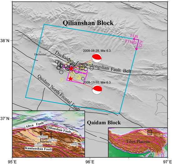
2. Data and Layered Model
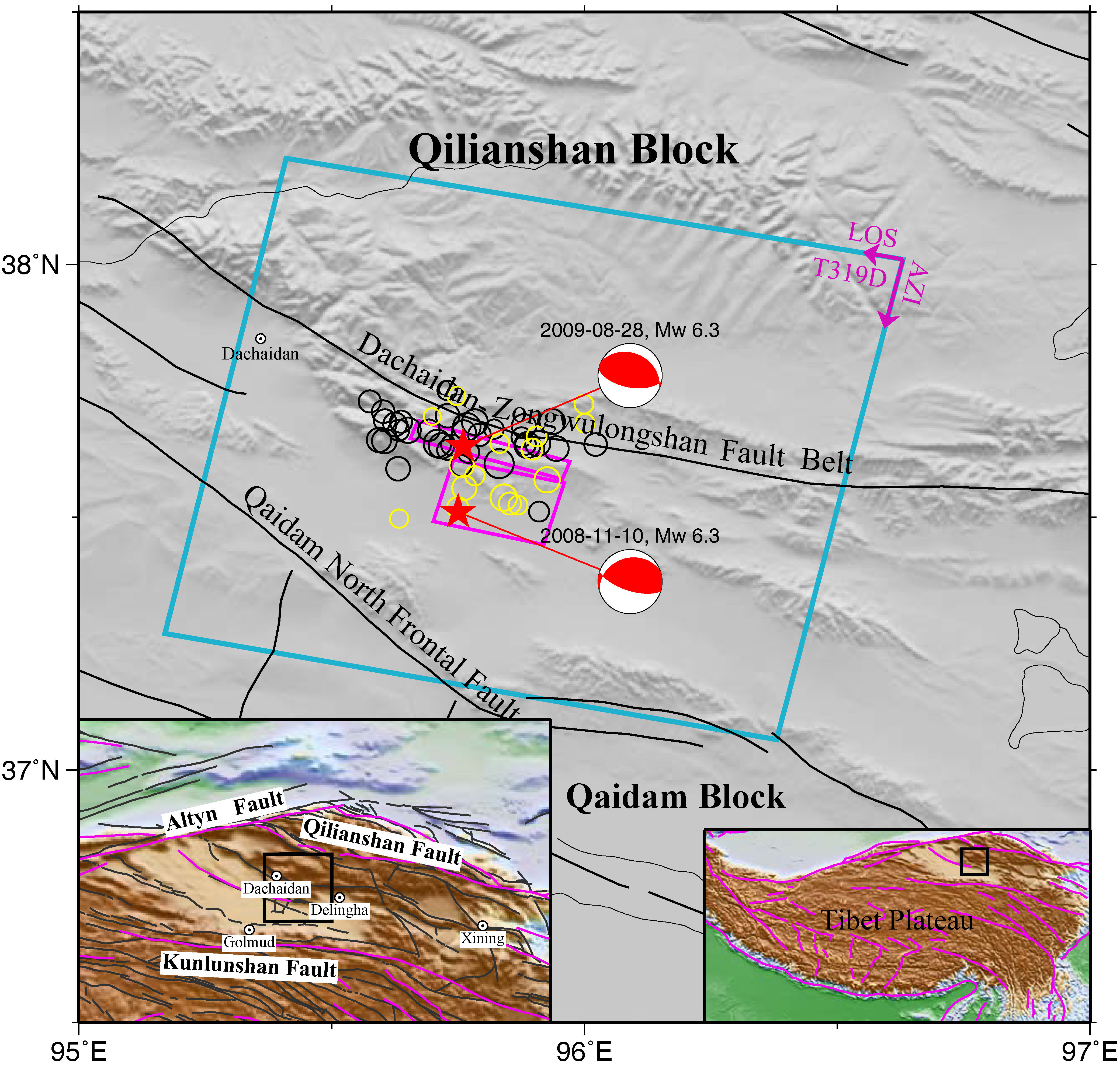
2.1. Data
2.2. Layered Model
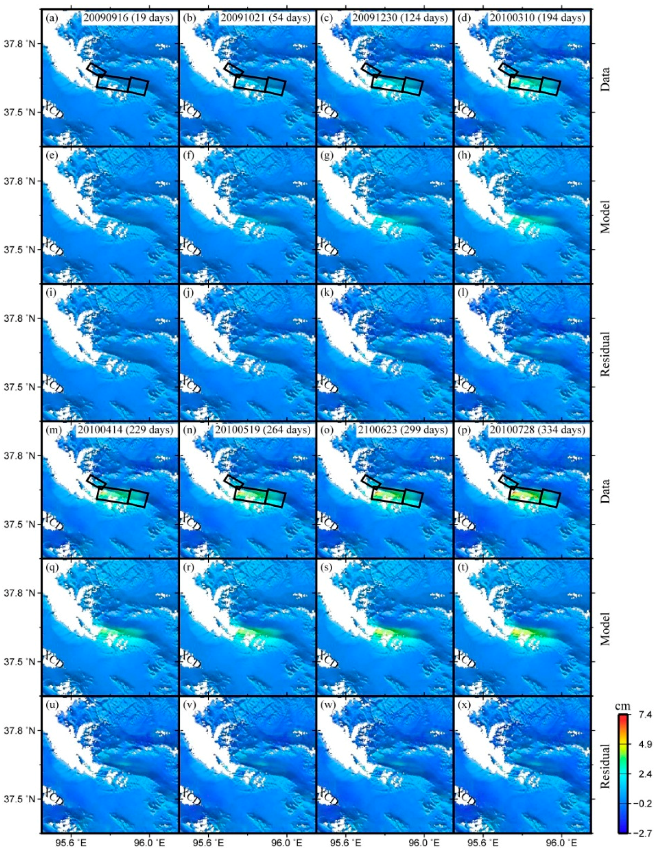
3. Modeling Method
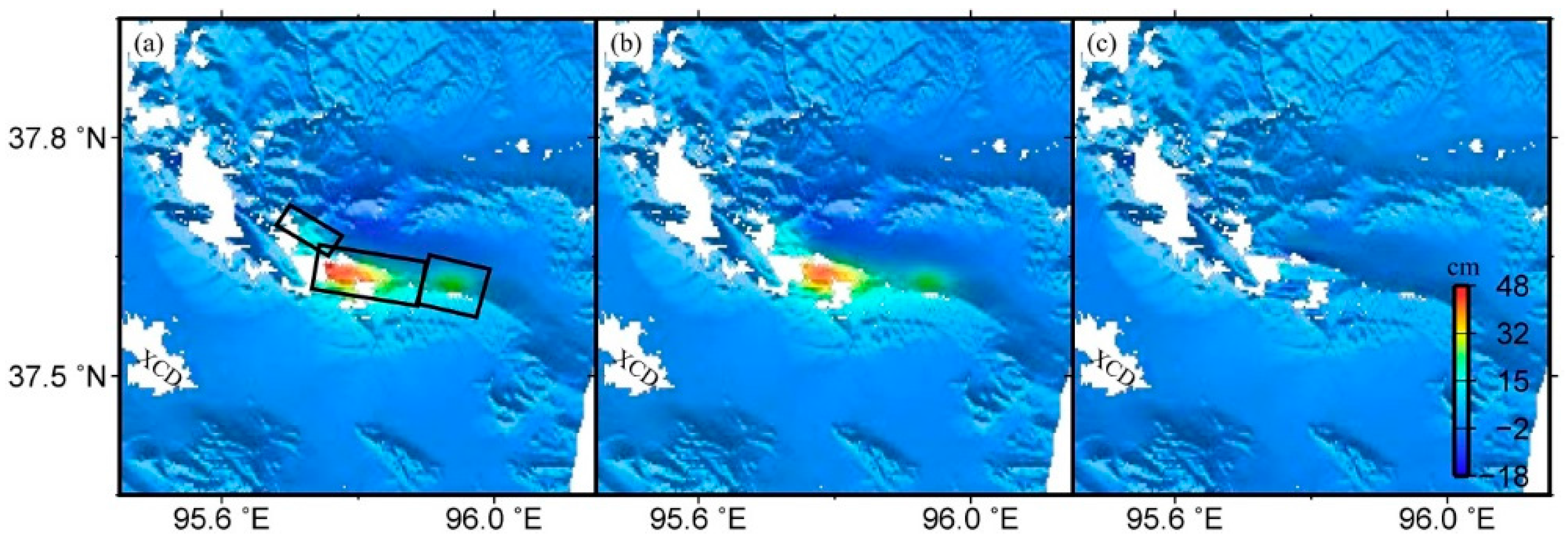
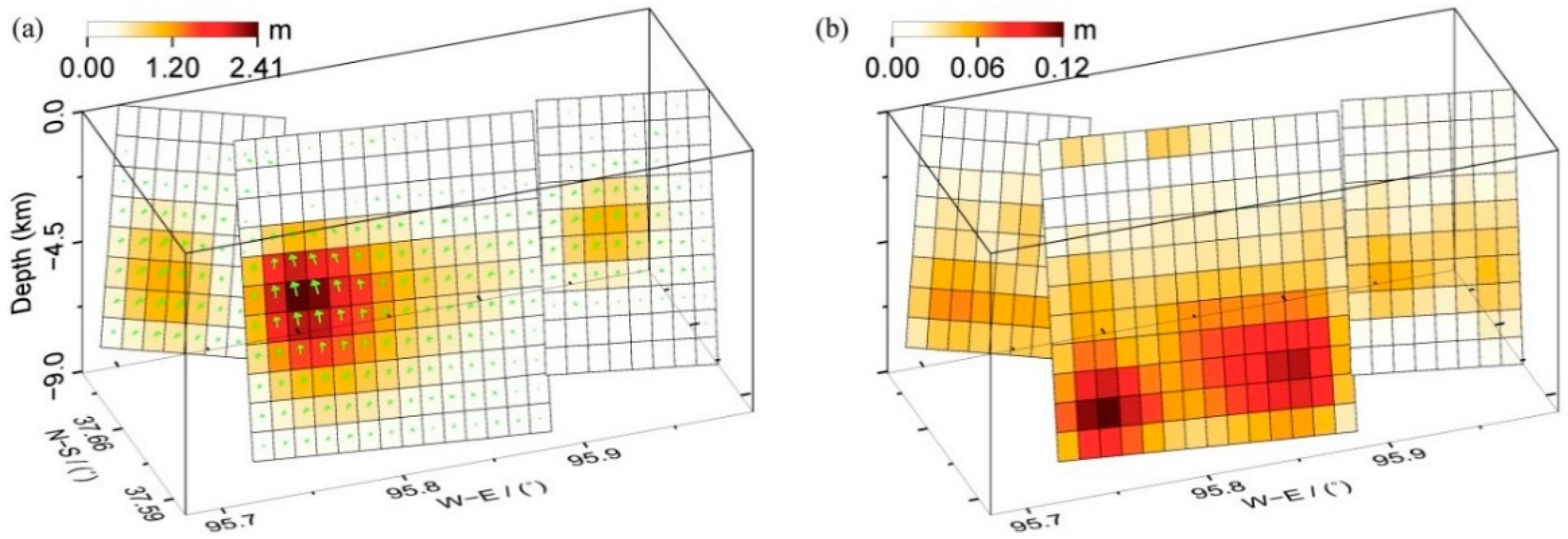
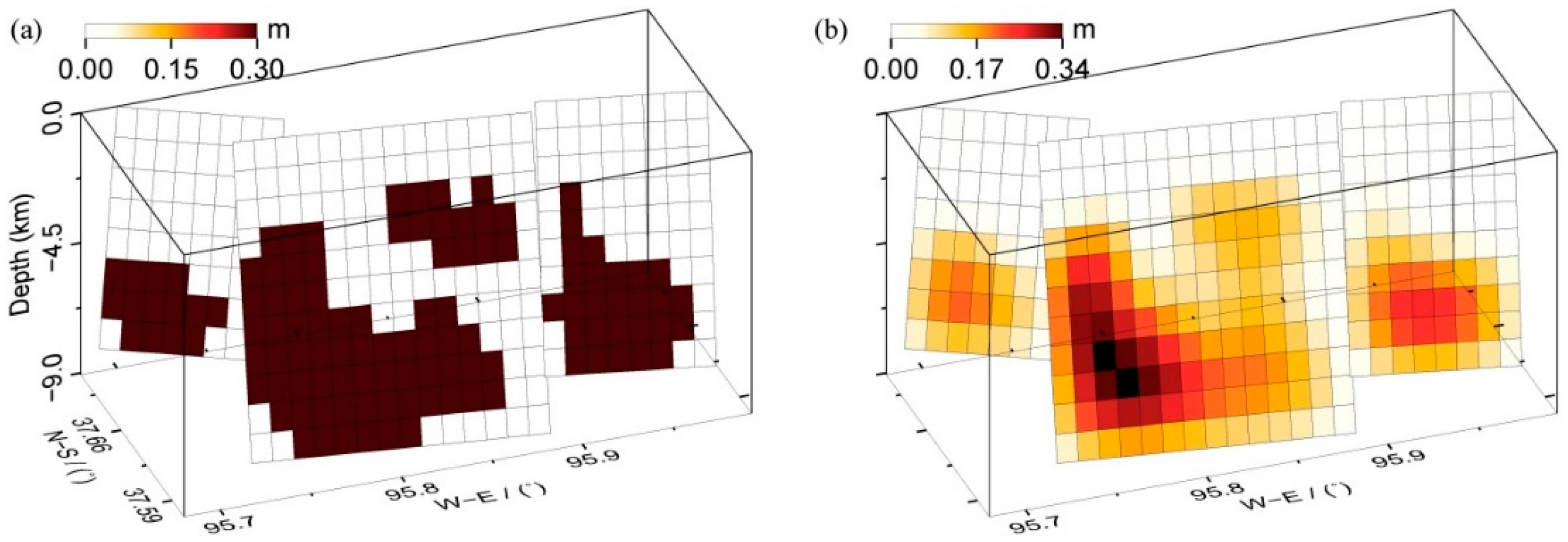
4. Coseismic Slip in the Layered Model
5. Time-Dependent Afterslip and Viscosity
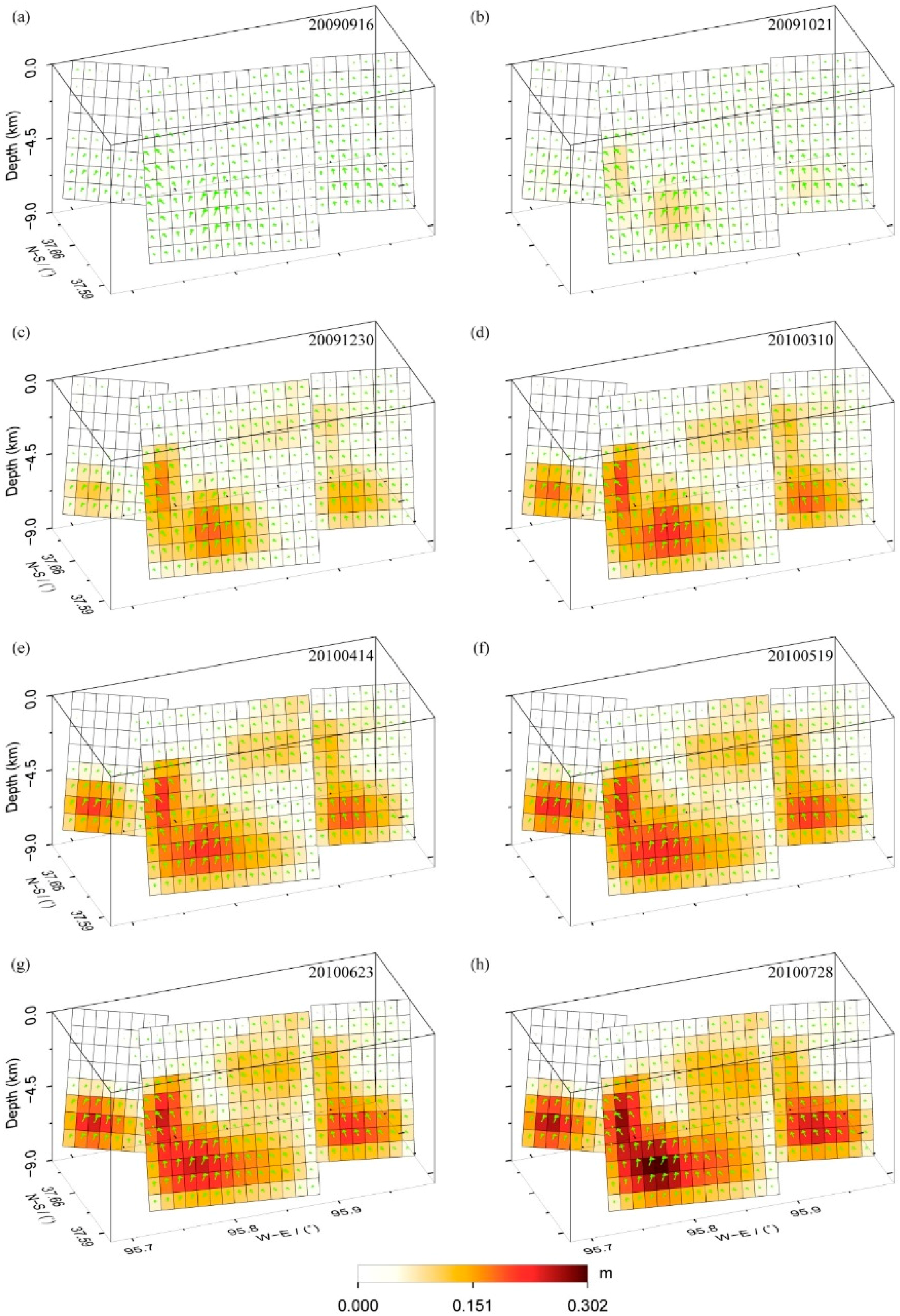
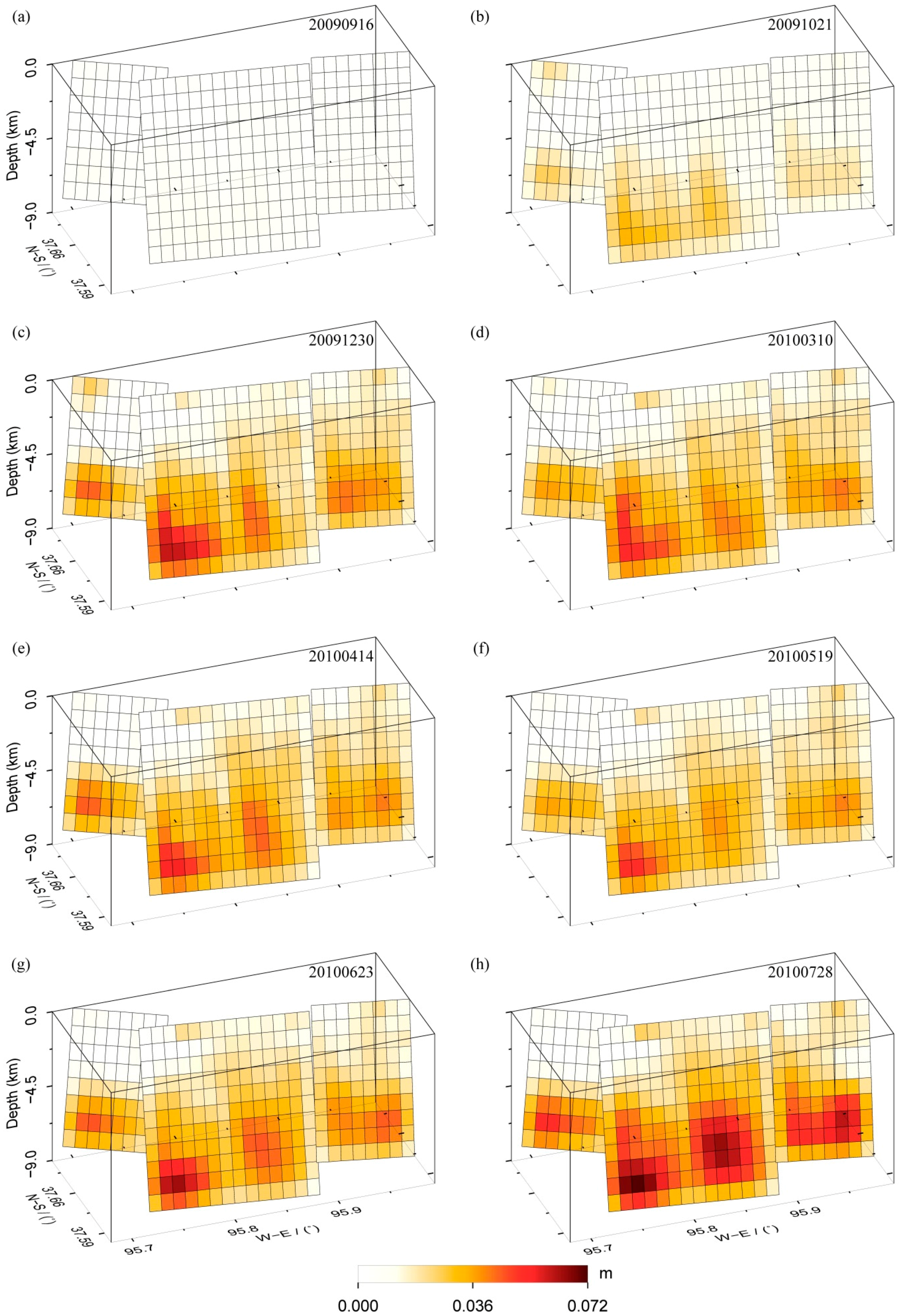
5.1. Time-Dependent Afterslip
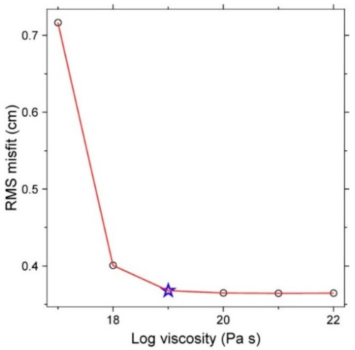
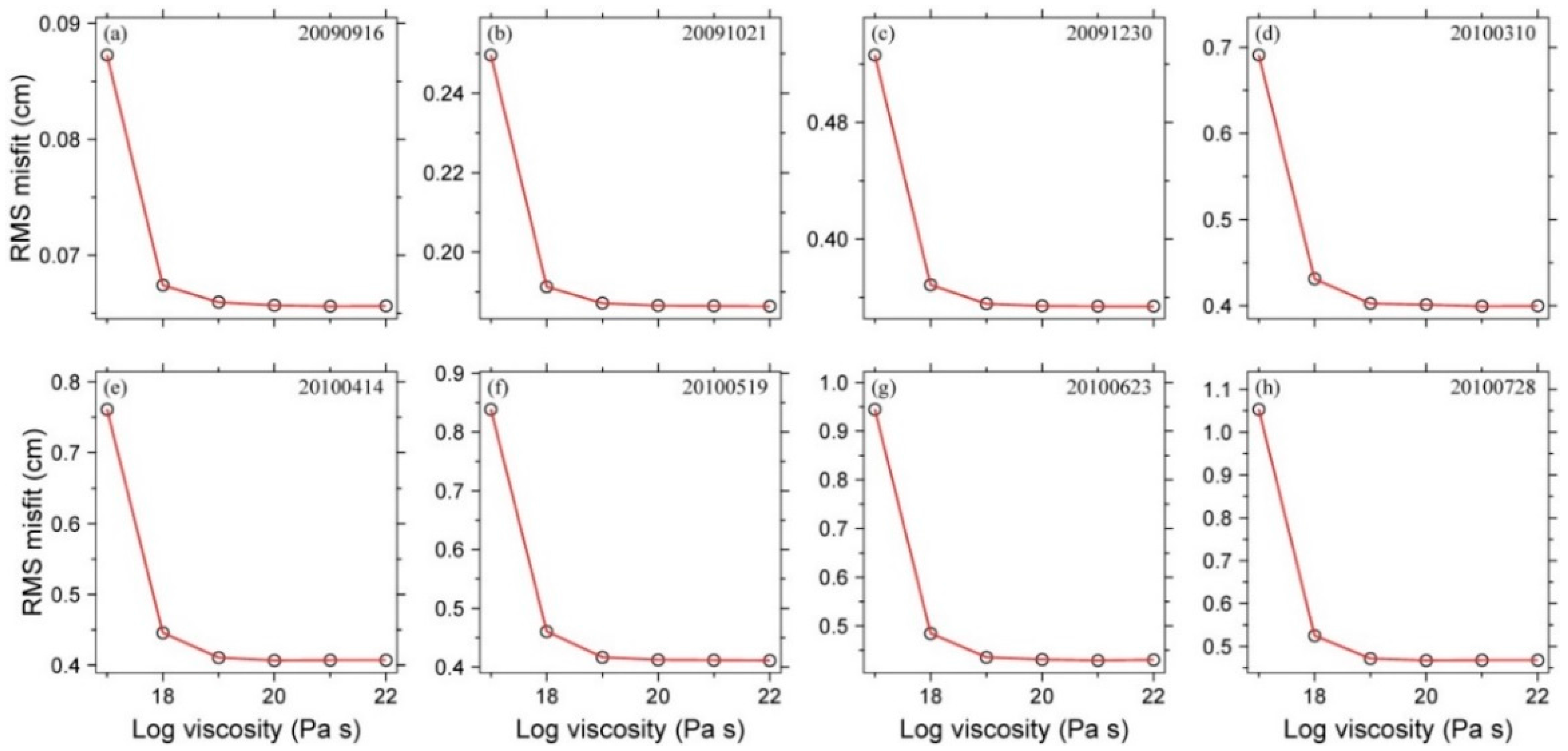
5.2. Viscosity
6. Discussion
6.1. Comparison of Inversion Results from Different Methods
6.2. Depth of Afterslip for the 2009 DCD Earthquake
6.3. Viscosity Structure Beneath the Qaidam Basin
7. Conclusions
Acknowledgments
Author Contributions
Conflicts of Interest
Abbreviations
| DCD | Dachaidan |
| NWW | northwestern-west |
| SEE | southeastern-east |
| GPS | Global Positioning System |
| InSAR | Interferometric Synthetic Aperture Radar |
| ASAR | Advanced Synthetic Aperture Radar |
| USGS | United States Geological Survey |
| XCD | Xiaochaidan |
| LOS | line-of-sight |
| RMS | root mean square |
References
- Elliott, J.; Parsons, B.; Jackson, J.; Shan, X.; Sloan, R.; Walker, R. Depth segmentation of the seismogenic continental crust: The 2008 and 2009 Qaidam earthquakes. Geophys. Res. Lett. 2011, 38. [Google Scholar] [CrossRef] [Green Version]
- Liu, W.; Wang, P.; Ma, Y.; Chen, Y. Relocation of Dachaidan Ms 6.4 earthquake sequence in Qinghai province in 2009 using the double difference location method. Plateau Earthq. Res. 2011, 23, 24–26. [Google Scholar]
- Liu, Y.; Xu, C.; Wen, Y.; Fok, H.S. A new perspective on fault geometry and slip distribution of the 2009 Dachaidan Mw 6.3 earthquake from InSAR observations. Sensors 2015, 15, 16786–16803. [Google Scholar] [CrossRef] [PubMed]
- USGS. Magnitude 6.2—Northern Qinghai, China. Available online: http://earthquake.usgs.gov/earthquakes/eqinthenews/2009/us2009kwaf/ (accessed on 23 May 2016).
- Deng, Q.; Zhang, P.; Ran, Y.; Yang, X.; Min, W.; Chu, Q. Basic characteristics of active tectonics of China. Sci. China Ser. D 2003, 46, 356–372. [Google Scholar]
- Zhang, P.; Deng, Q.; Zhang, G.; Ma, J.; Gan, W.; Min, W.; Mao, F.; Wang, Q. Active tectonic blocks and strong earthquakes in the continent of China. Sci. China Ser. D 2003, 46, 13–24. [Google Scholar]
- Reilinger, R. Evidence for postseismic viscoelastic relaxation following the 1959 M = 7.5 Hebgen Lake, Montana, earthquake. J. Geophys. Res. 1986, 91, 9488–9494. [Google Scholar] [CrossRef]
- Pollitz, F.F.; Peltzer, G.; Bürgmann, R. Mobility of continental mantle: Evidence from postseismic geodetic observations following the 1992 Landers earthquake. J. Geophys. Res. 2000, 105, 8035–8054. [Google Scholar] [CrossRef]
- Pollitz, F.F.; Wicks, C.; Thatcher, W. Mantle flow beneath a continental strike-slip fault: Postseismic deformation after the 1999 Hector Mine earthquake. Science 2001, 293, 1814–1818. [Google Scholar] [CrossRef] [PubMed]
- Tronin, A.A. Satellite remote sensing in seismology. Remote Sens. 2009, 2, 124–150. [Google Scholar] [CrossRef]
- Wen, Y.; Li, Z.; Xu, C.; Ryder, I.; Bürgmann, R. Postseismic motion after the 2001 Mw 7.8 Kokoxili earthquake in Tibet observed by InSAR time series. J. Geophys. Res. 2012, 117. [Google Scholar] [CrossRef]
- Xu, C.; Fan, Q.; Wang, Q.; Yang, S.; Jiang, G. Postseismic deformation after 2008 Wenchuan Earthquake. Surv. Rev. 2014, 46, 432–436. [Google Scholar] [CrossRef]
- Spinler, J.C.; Bennett, R.A.; Walls, C.; Lawrence, S.; González García, J.J. Assessing long-term postseismic deformation following the M7.2 4 April 2010, El Mayor-Cucapah earthquake with implications for lithospheric rheology in the Salton Trough. J. Geophys. Res. 2015, 120, 3664–3679. [Google Scholar] [CrossRef]
- Xu, B.; Xu, C. Numerical simulation of influences of the earth medium’s lateral heterogeneity on co-and post-seismic deformation. Geod. Geodyn. 2015, 6, 46–54. [Google Scholar] [CrossRef]
- Hamling, I.J.; Hreinsdóttir, S. Reactivated afterslip induced by a large regional earthquake, Fiordland, New Zealand. Geophys. Res. Lett. 2016, 43, 2526–2533. [Google Scholar] [CrossRef]
- Huang, M.-H.; Bürgmann, R.; Pollitz, F. Lithospheric rheology constrained from twenty-five years of postseismic deformation following the 1989 M w 6.9 Loma Prieta earthquake. Earth Planet. Sci. Lett. 2016, 435, 147–158. [Google Scholar] [CrossRef]
- Wen, Y.; Xu, C.; Liu, Y.; Jiang, G. Deformation and source parameters of the 2015 Mw 6.5 earthquake in Pishan, western China, from Sentinel-1A and ALOS-2 data. Remote Sens. 2016, 8. [Google Scholar] [CrossRef]
- Xu, C.; Xu, B.; Wen, Y.; Liu, Y. Heterogeneous fault mechanisms of the 6 October 2008 Mw 6.3 Dangxiong (Tibet) earthquake using Interferometric Synthetic Aperture Radar observations. Remote Sens. 2016, 8. [Google Scholar] [CrossRef]
- Evans, E.L.; Meade, B.J. Geodetic imaging of coseismic slip and postseismic afterslip: Sparsity promoting methods applied to the great Tohoku earthquake. Geophys. Res. Lett. 2012, 39. [Google Scholar] [CrossRef]
- Gan, W.; Zhang, P.; Shen, Z.-K.; Niu, Z.; Wang, M.; Wan, Y.; Zhou, D.; Cheng, J. Present-day crustal motion within the Tibetan Plateau inferred from GPS measurements. J. Geophys. Res. 2007, 112. [Google Scholar] [CrossRef]
- Liu, Y.; Xu, C.; Wen, Y.; He, P. The InSAR coseismic deformation observation and fault parameter inversion of the 2008 Dachaidan Mw 6.3 earthquake. Acta Geod. Cart. Sin. 2015, 44, 1202–1209. [Google Scholar]
- Feng, W. Modelling Co- and Post-Seismic Displacements Revealed by InSAR, and their Implications for Fault Behaviour. Ph.D. Thesis, University of Glasgow, Glasgow, UK, 2015. [Google Scholar]
- Liu, Y.; Xu, C.; Wen, Y.; Li, Z. Post-seismic deformation from the 2009 Mw 6.3 Dachaidan earthquake in the northern Qaidam Basin detected by small baseline subset InSAR technique. Sensors 2016, 16. [Google Scholar] [CrossRef] [PubMed]
- Peltzer, G.; Saucier, F. Present-day kinematics of Asia derived from geologic fault rates. J. Geophys. Res. 1996, 101, 27943–27956. [Google Scholar] [CrossRef]
- Massonnet, D.; Feigl, K.; Rossi, M.; Adragna, F. Radar interferometric mapping of deformation in the year after the Landers earthquake. Nature 1994, 369, 227–230. [Google Scholar] [CrossRef]
- Fialko, Y. Evidence of fluid-filled upper crust from observations of postseismic deformation due to the 1992 Mw 7. 3 Landers earthquake. J. Geophys. Res. 2004, 109. [Google Scholar] [CrossRef]
- Johanson, I.A.; Fielding, E.J.; Rolandone, F.; Burgmann, R. Coseismic and postseismic slip of the 2004 Parkfield earthquake from space-geodetic data. Bull. Seismol. Soc. Am. 2006, 96, 269–282. [Google Scholar] [CrossRef]
- Ryder, I.; Parsons, B.; Wright, T.J.; Funning, G.J. Post-seismic motion following the 1997 Manyi (Tibet) earthquake: InSAR observations and modelling. Geophys. J. Int. 2007, 169, 1009–1027. [Google Scholar] [CrossRef]
- Ryder, I.; Bürgmann, R.; Sun, J. Tandem afterslip on connected fault planes following the 2008 Nima-Gaize (Tibet) earthquake. J. Geophys. Res. 2010, 115, B03404. [Google Scholar] [CrossRef]
- Ryder, I.; Bürgmann, R.; Pollitz, F. Lower crustal relaxation beneath the Tibetan Plateau and Qaidam Basin following the 2001 Kokoxili earthquake. Geophys. J. Int. 2011, 187, 613–630. [Google Scholar] [CrossRef]
- Biggs, J.; Burgmann, R.; Freymueller, J.T.; Lu, Z.; Parsons, B.; Ryder, I.; Schmalzle, G.; Wright, T. The postseismic response to the 2002 M 7.9 Denali Fault earthquake: Constraints from InSAR 2003–2005. Geophys. J. Int. 2009, 176, 353–367. [Google Scholar] [CrossRef]
- Bie, L.; Ryder, I.; Nippress, S.E.J.; Bürgmann, R. Coseismic and post-seismic activity associated with the 2008 Mw 6.3 Damxung earthquake, Tibet, constrained by InSAR. Geophys. J. Int. 2014, 196, 788–803. [Google Scholar] [CrossRef]
- Diao, F.; Xiong, X.; Wang, R.; Zheng, Y.; Walter, T.R.; Weng, H.; Li, J. Overlapping post-seismic deformation processes: Afterslip and viscoelastic relaxation following the 2011 Mw 9.0 Tohoku (Japan) earthquake. Geophys. J. Int. 2014, 196, 218–229. [Google Scholar] [CrossRef]
- Brown, L.D.; Reilinger, R.E.; Holdahl, S.R.; Balazs, E.I. Postseismic crustal uplift near Anchorage, Alaska. J. Geophys. Res. 1977, 82, 3369–3378. [Google Scholar] [CrossRef]
- Shen, Z.K.; Jackson, D.D.; Feng, Y.; Cline, M.; Kim, M.; Fang, P.; Bock, Y. Postseismic deformation following the Landers earthquake, California, 28 June 1992. Bull. Seismol. Soc. Am. 1994, 84, 780–791. [Google Scholar]
- Savage, J.; Svarc, J. Postseismic deformation associated with the 1992 Mw = 7.3 Landers earthquake, southern California. J. Geophys. Res. 1997, 102, 7565–7577. [Google Scholar] [CrossRef]
- Hsu, Y.J.; Bechor, N.; Segall, P.; Yu, S.B.; Kuo, L.C.; Ma, K.F. Rapid afterslip following the 1999 Chi-Chi, Taiwan earthquake. Geophys. Res. Lett. 2002, 29, 1–4. [Google Scholar] [CrossRef]
- Chen, G.; Xu, X.; Zhu, A.; Zhang, X.; Yuan, R.; Klinger, Y.; Nocquet, J.-M. Seismotectonics of the 2008 and 2009 Qaidam earthquakes and its implication for regional tectonics. Acta Geol. Sin. 2013, 87, 618–628. [Google Scholar]
- Parsons, B.; Wright, T.; Rowe, P.; Andrews, J.; Jackson, J.; Walker, R.; Khatib, M.; Talebian, M.; Bergman, E.; Engdahl, E. The 1994 Sefidabeh (eastern Iran) earthquakes revisited: New evidence from satellite radar interferometry and carbonate dating about the growth of an active fold above a blind thrust fault. Geophys. J. Int. 2006, 164, 202–217. [Google Scholar] [CrossRef]
- An, C.; Song, Z.; Chen, G.; Chen, L.; Zhuang, Z.; Fu, Z.; Lu, Z.; Hu, J. 3-D shear velocity structure in north-west China. Chin. J. Geophys. 1993, 36, 317–325. [Google Scholar]
- Liu, W.; Zhang, X.; Hu, Y. Accurate location of Dachaidan Ms 6.3 earthquake sequence and earthquake tectonic using the double-difference earthquake location method. Plateau Earthq. Res. 2012, 24, 20–24. [Google Scholar]
- Liu, W.; Zhang, X.; Shi, Y.; Wen, Y.; Zhao, Y. Using green function database and quick moment tensor inversion calculating the focal mechanism solution of aftershocks of Dachaidan Ms 6.4 earthquake in 2008 in Qinghai province. Northwest. Seismol. J. 2012, 34, 154–160. [Google Scholar]
- Owens, T.J.; Zandt, G. Implications of crustal property variations for models of Tibetan plateau evolution. Nature 1997, 387, 37–43. [Google Scholar] [CrossRef]
- Berteussen, K.A. Moho depth determinations based on spectral ratio analysis of NORSAR long-period P waves. Phys. Earth Planet. Inter. 1977, 31, 313–326. [Google Scholar] [CrossRef]
- Wang, R.; Martin, F.L.; Roth, F. Computation of deformation induced by earthquakes in a multi-layered elastic crust-FORTRAN programs EDGRN/EDCMP. Comput. Geosci. 2003, 29, 195–207. [Google Scholar] [CrossRef]
- Wang, R.; Lorenzo-Martin, F.; Roth, F. PSGRN/PSCMP—A new code for calculating co-and post-seismic deformation, geoid and gravity changes based on the viscoelastic-gravitational dislocation theory. Comput. Geosci. 2006, 32, 527–541. [Google Scholar] [CrossRef]
- Wang, R.; Diao, F.; Hoechner, A. SDM—A geodetic inversion code incorporating with layered crust structure and curved fault geometry. In Proceedings of the EGU General Assembly, Vienna, Austria, 7–12 April 2013.
- Wen, Y.; Xu, C.; Liu, Y.; Jiang, G.; He, P. Coseismic slip in the 2010 Yushu earthquake (China), constrained by wide-swath and strip-map InSAR. Nat. Hazards Earth Syst. Sci. 2013, 13, 35–44. [Google Scholar] [CrossRef]
- Rosen, P.A.; Hensley, S.; Peltzer, G.; Simons, M. Updated repeat orbit interferometry package released. Eos Trans. AGU 2004, 85. [Google Scholar] [CrossRef]
- Wright, T.J.; Lu, Z.; Wicks, C. Source model for the Mw 6.7, 23 October 2002, Nenana Mountain earthquake (Alaska) from InSAR. Geophys. Res. Lett. 2003, 30. [Google Scholar] [CrossRef]
- Lin, Y.-n.N.; Sladen, A.; Ortega-Culaciati, F.; Simons, M.; Avouac, J.-P.; Fielding, E.J.; Brooks, B.A.; Bevis, M.; Genrich, J.; Rietbrock, A. Coseismic and postseismic slip associated with the 2010 Maule Earthquake, Chile: Characterizing the Arauco Peninsula barrier effect. J. Geophys. Res. 2013, 118, 3142–3159. [Google Scholar] [CrossRef] [Green Version]
- Marone, C.J.; Scholtz, C.; Bilham, R. On the mechanics of earthquake afterslip. J. Geophys. Res. 1991, 96, 8441–8452. [Google Scholar] [CrossRef]
- Bürgmann, R.; Ergintav, S.; Segall, P.; Hearn, E.H.; McClusky, S.; Reilinger, R.E.; Woith, H.; Zschau, J. Time-dependent distributed afterslip on and deep below the Izmit earthquake rupture. Bull. Seismol. Soc. Am. 2002, 92, 126–137. [Google Scholar] [CrossRef]
- Pollitz, F.F.; Bürgmann, R.; Thatcher, W. Illumination of rheological mantle heterogeneity by the M7.2 2010 El Mayor-Cucapah earthquake. Geochem. Geophys. Geosyst. 2012, 13. [Google Scholar] [CrossRef]
- Clark, M.K.; Royden, L.H. Topographic ooze: Building the eastern margin of Tibet by lower crustal flow. Geology 2000, 28, 703–706. [Google Scholar] [CrossRef]
- Cook, K.L.; Royden, L.H. The role of crustal strength variations in shaping orogenic plateaus, with application to Tibet. J. Geophys. Res. 2008, 113. [Google Scholar] [CrossRef]
- Bendick, R.; McKenzie, D.; Etienne, J. Topography associated with crustal flow in continental collisions, with application to Tibet. Geophys. J. Int. 2008, 175, 375–385. [Google Scholar] [CrossRef]
- Copley, A.; McKenzie, D. Models of crustal flow in the India-Asia collision zone. Geophys. J. Int. 2007, 169, 683–698. [Google Scholar] [CrossRef]
- Hilley, G.E.; Johnson, K.M.; Wang, M.; Shen, Z.K.; Burgmann, R. Earthquake-cycle deformation and fault slip rates in northern Tibet. Geology 2009, 37, 31–34. [Google Scholar] [CrossRef]
- England, P.C.; Walker, R.T.; Fu, B.; Floyd, M.A. A bound on the viscosity of the Tibetan crust from the horizontality of palaeolake shorelines. Earth Planet. Sci. Lett. 2013, 375, 44–56. [Google Scholar] [CrossRef]
- Zhang, C.; Cao, J.; Shi, Y. Studying the viscosity of lower crust of Qinghai-Tibet Plateau according to post-sesimic deformation. Sci. China Ser. D 2008, 38, 1250–1257. [Google Scholar]


| Date No. | Date | T a (Days) | Alpha b (km) | Sigma c (cm) | RMS d (cm) | Statistic Value e (cm) |
|---|---|---|---|---|---|---|
| 1 | 16 September 2009 | 19 | 4.72 | 0.07 | 0.07 | 0.31/0.37 |
| 2 | 21 October 2009 | 54 | 4.72 | 0.20 | 0.19 | |
| 3 | 30 December 2009 | 124 | 4.72 | 0.36 | 0.36 | |
| 4 | 10 March 2010 | 194 | 4.24 | 0.36 | 0.40 | |
| 5 | 14 April 2010 | 229 | 4.40 | 0.35 | 0.41 | |
| 6 | 19 May 2010 | 264 | 4.84 | 0.34 | 0.42 | |
| 7 | 23 June 2010 | 299 | 5.56 | 0.37 | 0.44 | |
| 8 | 28 July 2010 | 334 | 6.12 | 0.46 | 0.47 |
| Layer No. | Thickness (km) | Vp (km/s) | Vs (km/s) | Density (kg/m3) | Viscosity (Pa·s) |
|---|---|---|---|---|---|
| 1 | 8 | 5.19 | 3.00 | 2430.8 | N/A |
| 2 | 15 | 6.31 | 3.65 | 2790.6 | N/A |
| 3 | Infinite | 6.06 | 3.50 | 2707.6 | Variable |
| Method | Maximum Slip a (m) | Moment a (1016 N·m) | Mw a | Viscosity (Pa·s) |
|---|---|---|---|---|
| 1 | 0.302 | 90.68 | 5.938 | 1 × 10¹⁹ |
| 2 | 0.298 | 90.22 | 5.937 | 1 × 10¹⁹ |
| 3 | 0.274 | 87.26 | 5.927 | N/A |
© 2016 by the authors; licensee MDPI, Basel, Switzerland. This article is an open access article distributed under the terms and conditions of the Creative Commons Attribution (CC-BY) license (http://creativecommons.org/licenses/by/4.0/).
Share and Cite
Liu, Y.; Xu, C.; Li, Z.; Wen, Y.; Chen, J.; Li, Z. Time-Dependent Afterslip of the 2009 Mw 6.3 Dachaidan Earthquake (China) and Viscosity beneath the Qaidam Basin Inferred from Postseismic Deformation Observations. Remote Sens. 2016, 8, 649. https://0-doi-org.brum.beds.ac.uk/10.3390/rs8080649
Liu Y, Xu C, Li Z, Wen Y, Chen J, Li Z. Time-Dependent Afterslip of the 2009 Mw 6.3 Dachaidan Earthquake (China) and Viscosity beneath the Qaidam Basin Inferred from Postseismic Deformation Observations. Remote Sensing. 2016; 8(8):649. https://0-doi-org.brum.beds.ac.uk/10.3390/rs8080649
Chicago/Turabian StyleLiu, Yang, Caijun Xu, Zhenhong Li, Yangmao Wen, Jiajun Chen, and Zhicai Li. 2016. "Time-Dependent Afterslip of the 2009 Mw 6.3 Dachaidan Earthquake (China) and Viscosity beneath the Qaidam Basin Inferred from Postseismic Deformation Observations" Remote Sensing 8, no. 8: 649. https://0-doi-org.brum.beds.ac.uk/10.3390/rs8080649