Airborne Lidar Estimation of Aboveground Forest Biomass in the Absence of Field Inventory

Abstract

The scientific community involved in the UN-REDD program is still reporting large uncertainties about the amount and spatial variability of CO₂ stored in forests. The main limitation has been the lack of field samplings over space and time needed to calibrate and convert remote sensing measurements into aboveground biomass (AGB). As an alternative to costly field inventories, we examine the reliability of state-of-the-art lidar methods to provide direct retrieval of many forest metrics that are commonly collected through field sampling techniques (e.g., tree density, individual tree height, crown cover). AGB is estimated using existing allometric equations that are fed by lidar-derived metrics at either the individual tree- or forest layer-level (for the overstory or underneath layers, respectively). Results over 40 plots of a multilayered forest located in northwest Portugal show that the lidar method provides AGB estimates with a relatively small random error (RMSE = of 17.1%) and bias (of 4.6%). It provides local AGB baselines that meet the requirements in terms of accuracy to calibrate satellite remote sensing measurements (e.g., the upcoming lidar GEDI (Global Ecosystem Dynamics Investigation), and the Synthetic Aperture Radar (SAR) missions NISAR (National Aeronautics and Space Administration and Indian Space Research Organization SAR) and BIOMASS from the European Space Agency, ESA) for AGB mapping purposes. The development of similar techniques over a variety of forest types would be a significant improvement in quantifying CO₂ stocks and changes to comply with the UN-REDD policies.

1. Introduction

Measuring and monitoring aboveground biomass (AGB) has become an important research topic in the last decade as a result of its importance within the carbon cycle, as well as for its relevance to the international climate negotiations [1]. In 2009, the United Nations Framework Convention on Climate Change (UNFCCC) established the MRV (measuring, reporting and verification) guidelines for evaluating forest carbon stocks in the context of implementing REDD (Reduced Emissions from Deforestation and forest Degradation [2]). The components of MRV include: (i) measuring the extent and change in forest area; (ii) reporting carbon stocks and emissions; and (iii) verifying the findings and implementation of REDD activities.

The existing and upcoming remote sensing sensors are important tools to quantify the magnitude and spatial distribution of AGB at the regional, national and global scales. Nonetheless, as far as the AGB estimation is concerned, the cutting edge remote techniques are still highly dependent on the availability, quality and quantity of traditional local-scale field inventory systems [3]. Briefly, AGB is assessed from remote sensing data through a two-stage procedure. At the first stage, remote sensing measures or “metrics” are related to AGB, typically via regression models, with associated field-derived AGB. At the second stage, the resulting AGB regression models are used to convert local-scale estimates into continuous AGB maps over larger areas [4,5]. The success of this approach strongly depends on the amount and quality of field-derived AGB. In most national and regional inventories, the plots are small in size and have significant uncertainty in location that may introduce large errors in calibrating the plot-level lidar metrics. This problem has been observed in most forest types globally [6,7,8]. In addition, the paucity of field inventory plots in most of the unmanaged forests due to the difficulty of the access and cost of establishing large plots has been a source of uncertainty in the use of regression model techniques [9,10]. Reducing such uncertainty would require the establishment of larger and more accurately located plots in global forests. It would imply, as well, changing the protocols of national inventory plots in temperate and boreal forests [1,11]. As a result, a fair accounting of carbon sequestration would need sophisticated field inventory systems able to assess and to monitor AGB at a broad range of geographical sites, with frequent temporal visits and high accuracy requirements [12]. Collecting such field measurements using traditional field techniques is not cost effective mainly in areas where there is little or no pre-existing inventory data, as well as in inaccessible areas and in areas that experience rapid changes in forest structure [3].

Here, we investigate the ability of airborne high-resolution lidar (light detection and ranging) techniques to estimate AGB without the need for those massive in situ measurements. We have been studying the ability of individual tree extraction methods to replace field sampling techniques over different complex forest ecosystems, such as the Mediterranean [13,14,15] and tropical rain forests [16]. We intend to assess their reliability to fulfill the requirements of quality in establishing robust AGB baselines that could be used to calibrate coarser remote sensing data, such as the measurements of the upcoming NASA spatial lidar missions GEDI (Global Ecosystem Dynamics Investigation, http://science.nasa.gov/missions/gedi/) and NISAR (National Aeronautics and Space Administration-Indian Space Research Organization Synthetic Aperture Radar, http://nisar.jpl.nasa.gov). Lidar samples would be used in a manner similar to field plots, but enabling the extension of forest sampling across larger areas. In this work, we focus on a Portuguese multilayered forest where the lidar data are used to estimate AGB by means of similar techniques to those commonly used in the field. Because AGB can only be measured directly through destructive sampling, it is usually estimated by means of allometric equations defined as a function of metrics that are easier to measure, such as stem diameter, tree height and forest layers’ cover. Recently, we developed methods that apply to high-resolution lidar data to directly retrieve most of the forest metrics required by allometric equations, such as tree density, individual tree height, crown depth, forest layers’ mean height and crown cover [13,14,15]. Similarly to field surveys carried out by the Portuguese authorities, the AGB is characterized at the individual tree level for the overstory and at the forest plot level for the understory and ground vegetation.

We first present the study site, which is covered by a Portuguese multilayered forest (Section 2.1). Secondly, we explain the approaches used to acquire forest metrics using either field sampling techniques (Section 2.2) or lidar data processing methods (Section 2.3). The AGB is estimated over 40 forest plots by means of three different techniques: (1) using field inventory measurements together with a set of allometric equations developed to apply to Portuguese forests (Section 2.4); (2) using lidar-derived forest metrics and the very same set of allometric equations (Section 2.5); and (3) using the traditional approach that establishes AGB regression models using both field inventory measurements and lidar point cloud metrics (Section 2.6). Regarding both (1) and (2), we first compare results for single layers (mature overstory, juvenile overstory, understory and ground vegetation; Section 3.1). Then, single layers are coherently summed up to assess the results at the forest plot level (Section 3.2). Finally, the latter are compared to the results found by the AGB regression model approach (Section 3.3). Conclusions are made in Section 4.

2. Materials and Methods

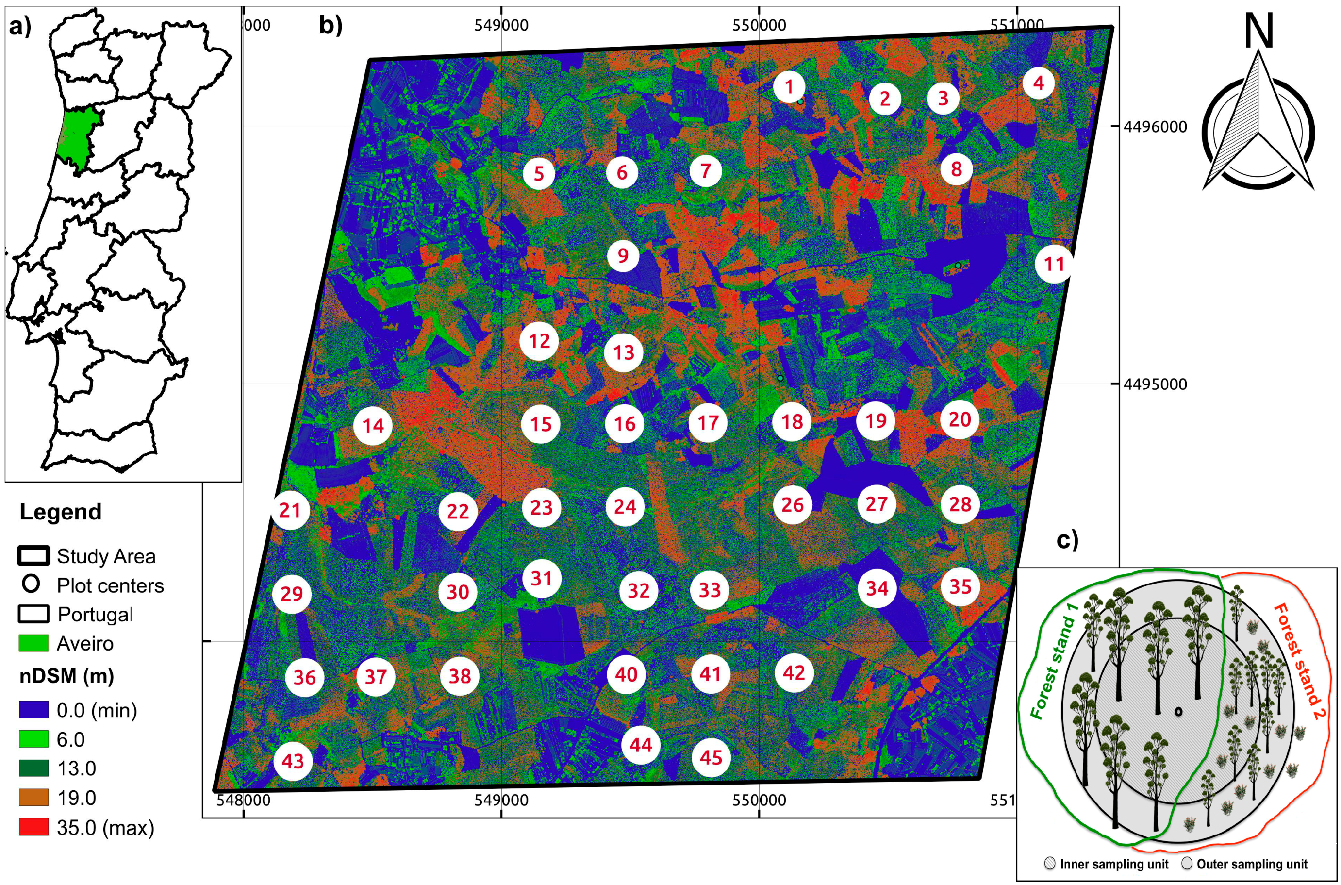
2.1. Study Site

The study area is located near the town of Águeda in northwest Portugal (40°36′N, 8°25′W) covering nearly 9 km² (Figure 1a). The altitude and slope range from 70–220 m and 2.5%–34.2%, respectively. The site is predominantly occupied by eucalyptus (Eucalyptus globulus Labill.), with some stands of maritime pine (Pinus pinaster Ait.), shrub and agricultural fields. The overstory is generally sparse and the understory well developed. The shrubby vegetation displays luxurious vegetation, typical of the Mediterranean forests. The underneath layer is mainly composed of suppressed trees (eucalyptus, maritime pine, acacia and oak), gorse bush (Ulex spp.), heath (Erica spp.), carquesia (Pterospartum spp.), gum cistus (Cistus spp.), blackberry (Rubus spp.), broom (Cytisus spp.), ferns and herbaceous plants.

2.2. Field Inventory

Forty-seven sampling units were defined in a systematic way following a forest inventory field protocol adapted from the Portuguese National Forest Inventory Manual (Figure 1b; [17]). Each sampling unit consists of two nested circles, an outer one (400 m²) and an inner one (200 m²), delineated using a distance measurer (Figure 1c). The study area is very heterogeneous because the forest belongs to many landowners (Figure 1b). As a result, a sampling unit may contain more than one forest stand (i.e., uniform plant communities in terms of species, age and spatial arrangement [18]), but only the stand where the center of the sampling unit is located was measured (Figure 1c). We define a forest plot as the area enclosed by the nested circles that comprise the forest stand of interest. Note that a forest plot and a sampling unit do not exactly overlap if the latter is populated by more than one forest stand.

Three plots out of the original forty-seven were discarded due to the impenetrable shrubby vegetation. Additionally, two plots occupied by maritime pine are not taken into account in this study because we do not dispose of allometric equations specific for the Portuguese territory. On the one hand, we cannot derive AGB directly from the lidar data because in the literature, there is no equation to convert individual tree height into AGB. On the other hand, there is also no stem diameter-tree height relationship that we could use to estimate stem diameter from tree height. This prevents us from using an existing stem diameter-AGB allometric equation that is commonly used in the framework of field inventories. Furthermore, the small number of trees surveyed in this experiment prevents us from deriving a robust stem diameter-tree height relationship specific for this study. Finally, two plots that were less than 1 year old are discarded because they are not meaningful in terms of AGB. As a result, 40 plots with eucalyptus are studied here. The age of the plots ranged from 1–13 years old. They were stratified into two age groups containing 10 juvenile plots (1–4 years) and 30 mature plots (>4 years). Juvenile plots are composed of either two layers (ground vegetation and juvenile overstory) or ground vegetation only. Mature plots may display three layers (ground vegetation, understory and overstory) or two only due to clearing activities for the removal of the understory vegetation.

The species was recorded for every single tree higher than 2 meters, as well as the diameter at breast height (dbh, cm), the tree height (th, m) and the crown base height (cbh, m). The dbh was measured using a caliper, whereas both th and cbh with a telescopic stick or a Vertex hypsometer. Finally, each tree was assigned to one class that defines its social status: dominant, codominant, dominated and suppressed trees. As far as understory and ground vegetation is concerned, it would be unfeasible to characterize every plant individually. Instead, they are characterized at the plot level by means of the layer mean height ($\overline{h}$, m), the crown cover (cc, %) and the dominance (d, %). The cc is defined as the total vertical projection area of plants’ crowns divided by the horizontal area of the observation unit on which trees are growing [15,19]. Overlapping crowns are not counted twice, and the crown area is defined by the outermost perimeter (envelop) of the crowns, including within crown gaps. Finally, d is simply cc discriminated by species, which means the name of the species present within the forest plots was recorded, as well. Following the field protocol, two field operators estimated the cc and d visually. When their estimation was similar, the average value was recorded; otherwise, they tried to reach an agreement. It is worth mentioning that the measurements at the single tree and plot level were carried out within the inner and outer circle, respectively (Figure 1c).

Information collected by a forest inventory usually has lower location accuracy than that provided by lidar systems. To improve it, a local geodetic network made of 41 pairs of GPS-derived points was built on the same map projection as the lidar data [20]. All plot centers, as well as the tree positions within the outer circle were surveyed using a total station theodolite. Finally, all of the data were integrated into a single 3D geometry.

2.3. Lidar Inventory

In this section, we describe the lidar dataset acquired over the study site (Section 2.3.1) and the methods used to extract forest metrics from the 3D lidar point cloud, i.e., the lidar forest metrics inventory (Section 2.3.2). These methods were published in Ferraz et al. [14] and Ferraz et al. [15], and their reliability to retrieve relevant forest metrics was already assessed. As a result, they are only briefly described here. Thus, instead of focusing on the methods themselves, our effort is directed at analyzing their reliability for the extraction of the forest metrics that are further used in AGB estimates (e.g., tree density, tree height, forest layers mean height and crown cover).

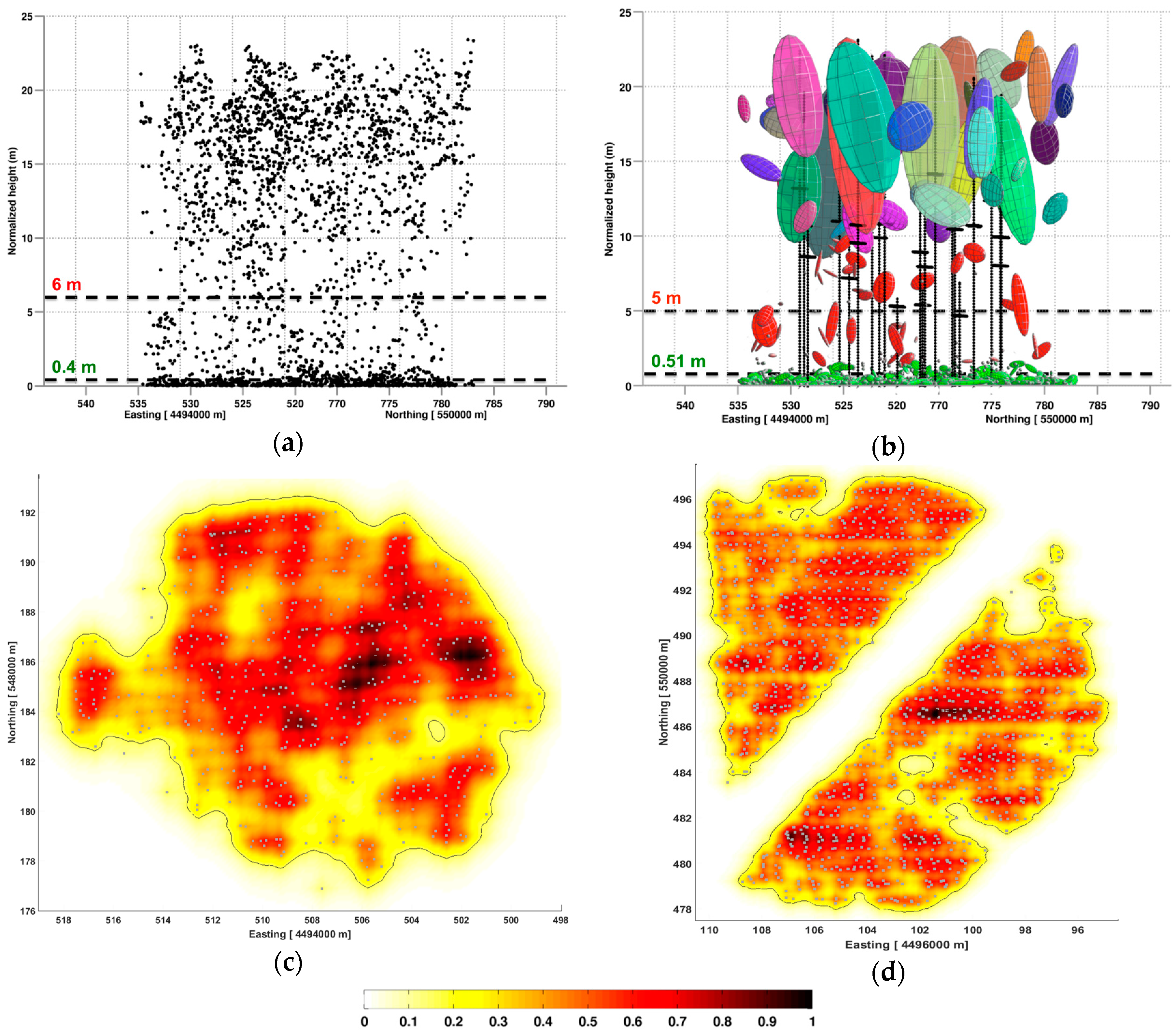
2.3.1. Lidar Data Measurements

The lidar data were acquired on 14 July 2008, in a full-waveform mode using a LiteMapper 5600. The footprint and the scan angle have the values 0.3 m and ±22.5°, respectively. A strip overlap of 70% guaranteed “wall-to-wall” coverage. With a single run pulse density of 3.3 points per square meter (pts/m²), the final average pulse density within each forest plot is 9.5 pts/m² (min = 4.7, max = 15.5, $\sigma$ = 1.9 pts/m²). The photons corresponding to each pulse were reflected by the different features of the landscape and recorded into a waveform structure. The digitized waves were processed using the RiANALIZE software (http://www.riegl.com/products/software-packages/rianalyze/) in a workstation; each pulse gave rise to 1–5 lidar returns. The position and orientation of the platform, which are given by onboard GPS/IMU hybrid measurements, were corrected by analyzing overlapping laser strips from the calibration cross-strips. These parameters, together with the GPS measurements acquired during the flight using a reference ground station, provided a point cloud in the WGS84/UTM zone 29N coordinate system for further processing. Systematic height errors were finally removed by using field control data that spread all over the study area. To calculate the effective height of the objects in the scene, ground and vegetation returns were separated. A Delaunay triangulation was generated to produce a digital terrain model with 0.3-m spatial resolution that was used to normalize the point cloud. More details of this experiment concerning both the field inventory and lidar data can be found in Ferraz et al. [14] and Ferraz et al. [15].

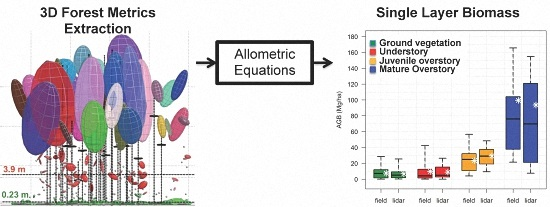
2.3.2. Forest Metrics Extraction

The forest metrics, such as the tree density, individual tree height, individual crown length and height of forest layers, are important to estimate AGB. With the exception of the latter, which was estimated using the approach published in Ferraz et al. [15], the metrics have been extracted using a method called adaptive mean shift (AMS3D) described in Ferraz et al. [14]. It applies directly to the lidar point cloud (Figure 2a) and provides 3D clusters of lidar points that correspond to individual vegetation features, such as shrubs or tree crowns. For visual purposes, we fit the minimum volume enclosing ellipsoid to each 3D cluster ([21]; Figure 2b). The AMS3D assigns every plant crown to a forest layer, namely ground vegetation, understory and overstory (green, red and randomly-colored ellipsoids). Therefore, the individual crown map shown in Figure 2b readily provides single layer forest metrics: tree density (number of ellipsoids within the forest plot normalized by its area), tree height (z coordinate of the highest lidar point assigned to a given 3D cluster), individual crown length (distance between the tree height and the lowest lidar point of the 3D cluster) and the forest layers mean height (the 50th height percentile of the lidar points assigned to juvenile overstory and understory and the 90th height percentile regarding the ground vegetation [22]). According to Ferraz et al. [15], the cc is computed for single layers using the lidar returns assigned to juvenile overstory, understory and ground vegetation. A statistical tool called kernel density estimators (KDE) was used to transform discrete measurements, i.e., lidar points, into continuous smooth surfaces called canopy density models (CDM). The later are probabilistic maps that calculate the probability of the occurrence of vegetation for every location in the forest based on the local spatial density of lidar points. Figure 2c,d show two different CDMs where such a probability for a given area is assigned to a value within the range [0, 1] (color bar in Figure 2). Then, the outermost perimeter of plants crowns (black contours in both Figure 2c,d) is delineated by means of a probability density threshold below which no vegetation is expected. The threshold is automatically defined as a function of the point cloud density for a given forest layer (for more details, refer to [15]). Finally, cc is computed as the ratio between the area covered by the plants’ crowns to the area of the forest plot.

In the following, we briefly describe the results concerning the forest metrics extraction found by Ferraz et al. [14,15]. Similar to field-based techniques, the mature forest overstory is characterized at the individual tree level through tree density, th and cbh, whereas the juvenile overstory, understory and ground vegetation at the forest plot level through $\overline{h}$ and cc. Regarding the density of mature overstory trees, the AMS3D approach can detect 438 trees out of 649 (67.5%). These trees are referred to as correctly-detected trees (CD). The CD success rate largely depends on the crown location in the forest canopy with 98.6%, 85.2%, 61.4% and 12.8% for dominant, codominant, dominated and suppressed eucalyptus trees, respectively. Conversely, 9.2% of the trees within the AMS3D maps correspond to false positive trees, i.e., fictitious trees that are hereafter called incorrectly-detected (ID) trees. This means that the AMS3D had extracted 60 trees that do not exist in the field due to either over-segmentation (a single crown was wrongly split into two) or the edge effect (tree stems outside the plot boundary have portions of their crowns extent within the plot boundary). Scatter plots of predicted versus observed th and cbh of CD trees show that the AMS3D explains better the variability associated with th (R² = 0.96%, RMSE = 0.86 m) than with the cbh (R² = 0.69%, RMSE = 2.48 m). Note that cl is obtained by subtracting cbh from th.

The juvenile overstory, understory and ground vegetation were validated at the forest plot level by means of $\overline{h}$ and cc. The comparison between observed and predicted $\overline{h}$ gives rise to satisfactory RMSE (0.31 m, 0.96 m and 0.15 m) with R² values of 0.92, 0.62 and 0.7 for juvenile overstory, understory and ground vegetation, respectively. Finally, the variability explained by the CDM-based approach regarding the cc equals 0.85, 0.85 and 0.84, respectively, whereas the corresponding RMSEs are 8.5%, 6.2% and 13.8%.

2.4. Aboveground Biomass Estimation Using Field Measurements

The forest layers’ AGBs are estimated using different allometric equations depending on the nature of the layers or the availability of field measurements for a given experiment (

Table 1. Allometric equations for AGB and $dbh$ (Equations (1)–(6) [23] and 7 [25], respectively). The acronyms $th$, $cl$, $dh$, $\overline{h}$, $cc$, $a$ and $\overline{bd}$ stand for tree height, crown length, dominant height, forest layer mean height, crown cover, area of the forest plot and weighted mean bulk density, respectively.

AGB (kg)
Individual trees	Stem	$w_w=0.0101\times dbh{}^{aw}\times t{h}^{1.3638}$		$aw=dh/\left(-0.6653+0.6243\times dh\right)$ if $dh\le 10.71$	(1)
				$aw=1.7788$ if $dh>10.71$
	Bark	$w_b=0.0006\times db{h}^{ab}\times t{h}^{1.0616}$		$ab=dh/\left(-0.6970+0.4586\times dh\right)$ if $dh\le 18.27$	(2)
				$ab=2.3784$ if $dh>18.27$
	Leaves	$w_l=0.0295\times db{h}^{al}\times {cl}^{0.6430}$		$al=dh/\left(-1.0312+0.7069\times dh\right)$ if $dh\le 7.39$	(3)
				$al=1.7627-0.01065\times dh$ if $dh>7.39$
	Branches	$w_{br}=0.0237\times dbh{}^{abr}\times cl{}^{0.6067}$		$abr=dh/\left(-0.913+0.7043\times dh\right)$ if $dh\le 8.83$	(4)
				$abr=1.664$ if $dh\le 8.83$
	Total	$w_t=w_w+w_b+w_l+w_{br}$			(5)
Forest layers		$w_{stratum}=\overline{h}\times cc\times a\times \overline{bd}$			(6)
dbh (cm)
Individual trees		$dbh=\frac{0.6073\times th}{1-0.0116\times th}$			(7)

). In this study, mature overstory AGB is first computed for individual trees (Equations (1)–(5)), and then, the results are summed up to estimate the total forest layer AGB. Conversely, AGB is directly calculated at the forest layer level for juvenile overstory, understory and ground vegetation (Equation (6)).

As far as individual trees are concerned, the allometric equations were established by destructive sampling of 441 eucalypti (Eucalyptus globulus Labill.) over 113 forest plots in Portugal [23]. Such equations depend on individual tree metrics, such as $dbh$, $th$ and crown length ($cl=th-cbh$), as well as on a forest plot-specific metric called dominant height ($dh$), which is defined as the mean height of the three tallest trees within a forest plot (Table 1). As for the forest layers, AGB is computed using Equation (6) as a function of the mean height ($\overline{h}$, meters), crown cover ($cc,\%$), area ($a,{\mathrm{m}}^2$) and weighted mean bulk density ($\overline{bd}$, kg·m⁻³). The bulk density is defined as the biomass per unit volume and depends on the species. Here, we defined $\overline{bd}$ as the weighted mean of the species bulk densities weighted by the species dominance (d, Section 2.2) that populate each forest plot layer. The bulk densities were obtained from Simões [24], who reports the reference values for most plant species that populate shrubby vegetation in Portugal.

2.5. Aboveground Biomass Estimation Using Lidar Measurements

The calculation of AGB using the lidar measurements is very similar to that of the field inventory because the AMS3D technique provides direct retrieval for most forest metrics required by the allometric equations shown in Table 1. Therefore, AGB for mature overstory is estimated at the individual tree level applying Equations (1)–(5). As mentioned in Section 2.3.2, the AMS3D provides all of the unknown variables except the dbh, the size of which is incompatible with the actual lidar spatial resolution employed for forestry applications, i.e., typically from 4 pt/m²–20 pt/m². As a result, the dbh is generally derived from th measurements using allometric equations [26]. Here, we apply Equation (7) established by Soares and Tomé [25] as a function of the very same field measurements used in this study that are described in Section 2.2. It is worth mentioning that we take advantage of the fact that only eucalyptuses live in the overstory. Otherwise, it would be necessary to discriminate tree species in order to select the adequate allometric equations.

Similarly to the field inventory technique, we calculate the AGB for juvenile overstory, understory and ground vegetation using Equation (6). As explained in Section 2.3.2, the AMS3D method provides single layer $\overline{h}$ measurements, whereas its cc is calculated using the CDM approach. Furthermore, a is simply the area of the forest plot that is calculated as the area of the convex hull that encloses all of the lidar points of a given plot (Section 2.2). The retrieval of the $\overline{bd}$ from the lidar data would imply the species identification within the underneath layers, which remains a scientific issue that would require further investigation and is discussed in Section 3. In this study, we used a layer-specific mean bulk density ($\widetilde{bd}$) that applies to the entire study area. Firstly, species that populate each layer were identified using the field inventory dataset (Section 2.3.2). The corresponding reference bulk densities given in Simões [24] were assigned to each species. The average of the bulk densities that populate each layer was computed in order to estimate the corresponding $\widetilde{bd}$. The values were 1.76, 2.21 and 2.46 kg·m⁻³ for juvenile overstory, understory and ground vegetation, respectively. Therefore, to estimate the AGB for single layers using the lidar approach, we set $\overline{bd}=\widetilde{bd}$ in Equation (6).

2.6. Aboveground Biomass Estimation Using Field and Lidar Measurements

A major advantage of our method with respect to the existing AGB regression model approach is that massive field inventory data are no longer required to calibrate and convert lidar point clouds’ metrics to AGB. Here, we compare their ability to explain the AGB variability over our study site in order to assess the contribution of our methodology in terms of AGB estimates’ accuracy with respect to the traditional approach. We developed an AGB regression model following Silva et al. [27]. Briefly, we first calculated 31 metrics from the 3D lidar point cloud (Table S1), according to each one of the forty forest plots (Section 2.2). Then, we used Pearson’s correlation coefficient (r) to identify highly correlated metrics and to exclude redundant predictors (r > 0.9). We selected the four most meaningful predictors using the “regsubset” function (package “leaps” in the R programming language [28]). It allows restraining the AGB regression model to be defined as a function of four metrics in the maximum, avoiding highly complex models. Next, we established a set of models by calculating a family of linear regressions defined as a function of one metric in the minimum and of four metrics in the maximum. The models have been ranked according to the minimum corrected Akaike information criterion (AIC) to select the AGB regression model that better explains the variability of our study site. Finally, the residuals of the model were analyzed graphically and tested for normality, as well as for heteroscedasticity. Results are reported using the leave-one-out cross-validation (loocv) technique. Please refer to Silva et al. [27] for more details on the regression model analysis.

3. Results and Discussion

Field- and lidar-derived aboveground estimates (AGB) are compared over 40 forest plots at two different scales. In Section 3.1, we analyze the results with respect to single forest layers, i.e., mature overstory, juvenile overstory, understory and ground vegetation. Then, single forest layers’ AGB estimates are summed up to assess results at the forest plot level (Section 3.2). Finally, we compare our results at the forest plot level to those obtained using a traditional lidar-based method that estimates AGB through a regression model technique (Section 3.3).

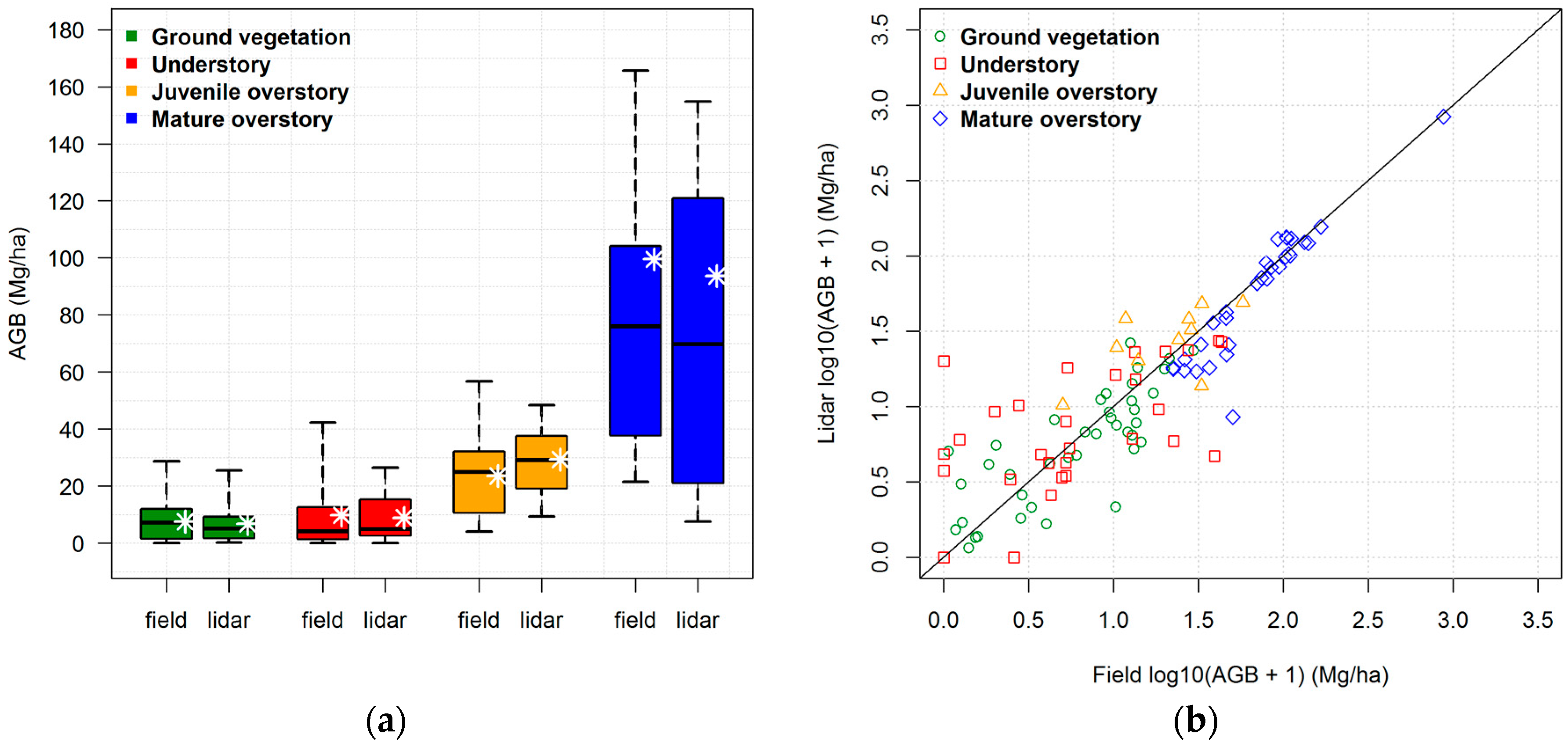
3.1. Aboveground Biomass at the Forest Layer Level

According to the field measurements, 7.9%, 7.7%, 6.2% and 78.3% of the total AGB is stored in ground vegetation, understory, juvenile overstory and mature overstory. The 40 field plots hold on average 7.5, 9.7, 23.5 and 99.5 megagrams (Mg) with standard deviations of 6.5, 12.3, 14.6 and 150.0 Mg, respectively. This is a strong indicator of the large study site heterogeneity. The mean bulk density ($\overline{bd}$) equals 2.5, 1.7 and 1.8 kg·m⁻³ for ground vegetation, understory and juvenile overstory, respectively. This means that ground vegetation species have higher bulk densities than those one can find within either the juvenile overstory or understory. Furthermore, ground vegetation and understory store a similar amount of biomass, but the latter is more heterogeneous mainly due to clearing activities (Figure 3a). However, most of the biomass is stored in the adult vegetation layer. Figure 1 and Figure 3a show the high forest structure variability in the horizontal and vertical component, respectively.

The box-and-whisker diagram illustrated in Figure 3a compares the main AGB statistics derived from field and lidar estimates at the forest layer level. It shows that the average AGB (white asterisks) is accurately estimated by the lidar approach for all of the forest layers. A similar conclusion can be made based on the median shown by the band inside each box. This is valid for mature overstory for which the mean and average are more than 20 Mg·ha⁻¹ apart from each other. This result indicates that our method performs well even over heterogeneous layers. The shape of the boxes shows that the AGB distribution is skewed concerning the juvenile overstory and the understory, whereas no such effect is visible over the mature overstory and ground vegetation. Nevertheless, the lidar data permitted capturing such characteristic of the AGB distribution for all forest layers, since boxes’ outlines are very similar. The extent of blue boxes indicates that mature overstory AGBs estimated applying the lidar approach show higher variability compared to field estimates. Briefly, by using the lidar approach, forest plots with higher AGB are slightly overestimated, whereas those with lower AGB are underestimated. This result is directly related to the under- and over-detection of individual trees. The extent of yellow and red boxes shows that the distribution of AGB regarding juvenile overstory and understory is well captured by the lidar approach, even if it tends to estimate higher values concerning the juvenile overstory. With respect to ground vegetation, lidar tends to estimate AGB with a lower variability, as the green boxes indicate.

Additionally, we use a scatter plot of the observed versus predicted AGB to quantify the strength of the relationship between field- and lidar -derived estimates for single layers (Figure 3b). Results are evaluated analyzing the coefficient of determination (R²), the absolute root mean square error (RMSE, Mg·ha⁻¹), the RMSE as a percentage (%), the absolute bias (Mg·ha⁻¹) and the bias as a percentage (

Table 2. Accuracy assessment statistics for field- and lidar-derived AGB both at the single layer level (rows denoted by mature overstory, juvenile overstory, understory and ground vegetation; Figure 3b) and at the forest plot level (row denoted by forest plot; Figure 4b). The rows denoted by forest plot* and forest plot** correspond to the results found by the AGB regression model approach (using a leave-one-out cross-validation (loocv)) taking into account all forest plots and without taking into account forest Plot #12, respectively (Figure 5b and Figure S1b). n corresponds to the number of plots, and the bias is calculated by averaging the differences between field and lidar AGB estimates. Negative bias values mean AGB under-estimation.

	n	R2	RMSE Mg·ha−1	RMSE (%)	Bias Mg·ha−1	Bias (%)
Single layer level
Mature overstory	30	0.99	18	18.1	−5.8	5.9
Juvenile overstory	10	0.38	13.3	56.7	+5.8	24
Understory	30	0.37	9.9	101.3	−0.8	8.9
Ground vegetation	40	0.65	4.1	53.3	−0.7	9.5
Forest plot level
Forest plot	40	0.99	16.3	17.1	−4.4	4.6
Forest plot level using a traditional regression model approach
Forest plot*	40	0.55	103.2	107.6	−9.4	9.9
Forest plot**	39	0.72	23.32	31.1	0.1	0.1

). In fact, we decided to calculate both RMSE and bias in terms of percentage regarding the mean AGB to control for differences in magnitudes between the different forest layers and to properly compare results between layers [1]. Accordingly, the percentage values are calculated by $\frac{RMSE}{\overline{AGB}}$ and $\frac{bias}{\overline{AGB}}$ where $\overline{AGB}$ represents the mean field-derived AGB for each layer.

Estimates for mature overstory, calculated as the sum of the individual trees’ AGB, was highly correlated (R² = 0.99) with the values derived from the field measurements, and we found a small bias of 5.9% (Figure 3b and Table 2). However, this result must be handled with caution. The dbh of the correctly-detected (CD) trees was computed by means of Equation (7) as a function of the lidar-derived th with R² = 0.78 and RMSE = 2.1 cm [14]. Then, the AGB of CD trees was calculated using Equations (1)–(5) (Table 1) with R² = 0.81 and RMSE = 22.63 kg. Therefore, lidar-derived AGB correlates better with biomass estimated at the layer level than at the individual tree level. In fact, mature overstory biomass is computed summing up the biomass from both CD and incorrectly-detected (ID) trees. It turns out that ID trees, i.e., false positives, generated by the AMS3D somewhat compensate the biomass held by undetected (UD) trees. Nevertheless, it does not explain the strong correlation at the plot-level since the percentage of UD trees (32.5%) is much higher than that of ID trees (9.2%). These results show that the lidar approach is able to detect the trees that hold most of the biomass within the forest plots. This means that many UD trees in our study area correspond to suppressed trees that store little biomass and are not meaningful in terms of AGB at the layer level.

As explained in Section 2.4 and Section 2.5, the AGB of juvenile overstory, understory and ground vegetation is estimated not at the individual tree level, but directly at the forest layer level (i.e., by means of Equation (6) instead of Equations (1)–(5); Table 1). Many factors explain the fact that the strength of the relationship is higher in the case of the mature overstory compared to the remaining forest layers. First, the field measurements were carried out at the plot level and are much less reliable than those of the mature overstory for which each plant specimen was surveyed. Secondly, both methods (AMS3D and CDM) introduce errors in the AGB estimation because they compute either $\overline{h}$ or cc with certain degrees of uncertainty (Section 2.3.2). Nevertheless, the lidar and field AGB estimation for ground vegetation are strongly correlated (R² = 0.65), whereas such a relationship is moderate for juvenile overstory and understory (R² = 0.38 and R² = 0.37, respectively). Results, which highly depend on the forest layer, are discussed individually in the following.

As far as juvenile overstory is regarded, the RMSE equals 56.7%, and a bias of 24% was observed. The latter is mainly a result of a systematic overestimation of the crown cover (cc, %) by the CDM method [15], since the retrieval of the juvenile overstory mean height ($\overline{h}$) is much more accurate [7]. It is still unclear whether the field-based cc was underestimated by the field crew or if the CDM is not able to accurately figure out the crown cover of juvenile eucalypti tree plots. With respect to the understory, the RMSE is very high (101.3%), but the bias is low (8.9%). This means that the results could be corrected taking into account some factors that degrade the results, namely the so-called shade effect introduced by the topmost vegetation on the laser beams. As a result, layers underneath may be under-sampled on the 3D point cloud compared to the topmost vegetation, namely the overstory. Additionally, many undergrowth-suppressed trees that populated this layer may not be dense enough to generate the number of lidar reflections needed to characterize the understory properly.

Surprisingly, the results concerning ground vegetation are much better than those of understory (R² = 0.65, RMSE = 53.5 and a bias of 9.5% only). The likely reason is that species that populated ground vegetation have denser crowns that increase the probability to give rise to a laser return. In fact, as stated in the first paragraph of this section, the species-specific bulk densities are higher for the typical ground vegetation plants than for those that occupy the juvenile overstory and understory. Therefore, higher bulk densities indicate denser plant material that increases the probability of causing a lidar return. Additionally, the average field-estimated cc equals 26.5%, 15.6% and 52.1%, for juvenile overstory, understory and ground vegetation, respectively. Similarly, because lidar measures forest structure by means of discrete measurements, the probability of a laser beam hitting a vegetation feature is higher over layers with higher cc. To sum up, results indicate that better estimates are achieved with respect to ground vegetation because it is a denser layer composed of plants with denser crowns. The shade effect seems to have less impact, since the worst results were obtained for juvenile overstory and understory that occupy higher layers.

Finally, it is worth noting that the results may be impacted as well by the fact that we are using different values for the bulk density in Equation (6), namely $\overline{bd}$ and $\widetilde{bd}$ for field- and lidar-derived AGB, respectively. The computation of $\overline{bd}$ implies knowledge about the species that populate each forest plot, as well as their dominance (Section 2.2). However, species identification from lidar data has been confined to the overstory layer and its effectiveness limited. Furthermore, to the best of our knowledge, the discrimination of species in either ground vegetation or understory has not been studied. Actually, some constraints limit the development of such a technique. Compared to the overstory, shrubby and herbaceous formations are generally more diverse, which greatly increases the complexity of the approach. In addition, due to the inability of lidar data to discriminate plants species in mixed forests, researchers have been discriminating species taking advantage of the synergy of lidar and hyperspectral imagery [29]. However, the vegetation underneath is not visible in such passive imagery. As a result, we believe that assessing $\overline{bd}$ from ancillary data is a reliable solution concerning the vegetation underneath. We suggest establishing averaged values well adapted to be applied to a specific forest area or eco-region. The plant species that are expected within an ecosystem can be assessed either by prior knowledge about the forest or derived from ecological studies, such as biodiversity mapping or the biogeographical distribution of plant species [30,31].

3.2. Aboveground Biomass at the Forest Plot Level

Single layer results for overstory, understory and ground vegetation were summed up to estimate AGB at the forest plot level. Figure 4a compares field and lidar estimates over the 40 forest plots using a box-and-whiskers diagram. The extent of the boxes and corresponding whiskers clearly shows that our approach is able to figure out the AGB variability over the study site with great accuracy. Furthermore, both mean and median AGB derived from the lidar approach are very close to the ones calculated from the field sampling, even if those statistics are very apart from each other, which is an indicator of the study site heterogeneity. Additionally, we examined the strength of the relationship between field and lidar estimates over the 40 forests plots as shown in Figure 4b and Table 2. The lidar-based approach is able to explain the AGB variability quite well (R² = 0.99) with a result similar to when we consider the mature overstory alone (Section 3.1). This result was expected because mature overstory holds the most biomass in our study area and therefore drives the AGB variability along the study site. Nevertheless, the absolute error (RMSE) was improved up to 1.7 Mg·ha⁻¹. More importantly, results in terms of RMSE (%) at the forest plot level were highly improved regarding the mature overstory: it decreases from 18.1% down to 0.4%. Additionally, a bias of −4.4 Mg·ha⁻¹ indicates a slight underestimation of the AGB that represents only 4.6% of the mean AGB for the 40 plots.

As a result, although results vary depending on the forest layer, our approach is able to retrieve unbiased estimates of AGB with low error at the forest plot level over a multilayered forest structure. This indicates that the AGB uncertainty can be highly reduced if forest layers are identified beforehand in order to estimate AGB at the individual layer level. Note that the widely-used AGB regression model approaches do not stratify vegetation into individual forest layers, which can explain the uncertainty observed over many multilayered forests. For instance, Garcia et al. [32] report RMSEs of 18.48, 15.98 and 9.7 Mg·ha⁻¹ for Spanish forests composed of black pines, Spanish junipers and holm oaks, respectively. In fact, the presence or absence of a dense underneath vegetation negatively impacts the lidar metrics’ variability (e.g., mean height, crown cover and height percentiles) and has an impact on the AGB estimates. More importantly, our approach removes the need for the massive field samplings that are required by the regression model approach to convert the lidar metric into AGB. This fact can highly decrease the cost of collecting accurate AGB baselines with high frequency. Finally, our approach was validated on very small forest plots, and it is well known that errors decline with increasing plot size [1].

3.3. Aboveground Biomass at the Forest Plot Level Using a Regression Model Approach

Table S2 shows the uncorrelated predictors, as well as the four most meaningful lidar metrics used in this study to establish a family of AGB regression models. The model that better explains the AGB variability was selected according to the minimum corrected Akaike information criterion (AIC). It is given by:

$$\log \left(AGB\right)=0.11h99-0.23hkurt-0.01hcv+3.41$$

(8)

where $log$ stands for natural logarithm, $h99$, $hkurt$ and $hcv$ correspond to the 99th percentile, the kurtosis metric and the coefficient of variation calculated using the height distribution of lidar returns, respectively (Section 2.6 and Table S1). Therefore, it turns out that the best model is defined as a function of three metrics out of the four most meaningful ones (Table S2).

By comparing the box-and-whisker diagrams in Figure 4a and Figure 5a, one can conclude that the regression model approach finds results very similar to our method in terms of the spread of the AGB estimates. The main difference is that our approach slightly underestimates the main statistics (mean, median, 25th and 75th percentiles) compared to the field estimates. Conversely, they are slightly overestimated by the regression model approach. The row denoted by forest plot* in Table 2 shows the performance of the AGB regression model approach using the leave-one-out cross-validation (loocv). It demonstrates that the AGB regression model poorly explains the AGB variability compared to our approach (R² = 0.52 vs. R² = 0.99, respectively). Furthermore, it gives rise to much higher RMSEs (103.2 and 16.3 Mg·ha⁻¹, respectively). These poor results are mainly due to the fact that the AGB regression model is unable to deal with the forest structure heterogeneity introduced by Forest Plot #12 (Figure 5b). The latter holds much more AGB than the remaining ones due to the existence of old growth eucalyptus trees. Unlikely, our approach deals much better with the forest heterogeneity because the AMS3D method (i) locally adapts to the forest structure and (ii) is able to correctly extract individual tree metrics. Therefore, a better strategy for the AGB regression model approach would require the definition of distinct models for areas displaying different forest structures. It would require a forest stratification technique to delineate communities of trees uniform in age and structure.

Due to the fact that only one forest plot comprises old growth trees, we decided to develop an additional AGB regression model that does not take into account Forest Plot #12 (Table S3 and Figure S1). The latter is similar to the former one (Equation (8)). Furthermore, they are both defined as a function of the very same lidar point cloud metrics:

$$\log \left(AGB\right)=0.11h99-0.22hkurt-0.01hcv+3.52$$

(9)

Results calculated using loocv are shown in the row denoted by forest plot** of Table 2. They significantly improved with respect to the regression model represented by Equation (8) (R² increases from 0.55–0.77, and the RMSE decreases from 103.2 down to 23.32 Mg·ha⁻¹), but they are poorer than the findings of our approach (Section 3.2, R² = 0.99 and RMSE = 16.3 Mg·ha⁻¹).

In summary, the results show that our approach better explains the AGB variability compared to the AGB regression models. These results may be due to the heterogeneity of our study area with respect to the forest vertical structure. On the one hand, the spatial heterogeneity in terms of underlying vegetation can impact the lidar metrics used in the AGB regression models, which limit their ability to explain the AGB variability. On the other hand, our method calculates the AGB for single layers and better deals with forest vertical structure variability.

4. Conclusions

We show that state-of-the-art lidar processing techniques that apply to high-resolution point clouds are reliable tools to estimate aboveground biomass (AGB) with high accuracy when compared to field-derived AGB even over complex structures, such as multilayered Mediterranean forests. Similarly to field techniques, our approach assesses AGB at the individual tree level for the understory layer and at the layer level for understory and ground vegetation. Moreover, it applies the very same allometric equations commonly used by field-based techniques to convert forest metrics estimates (e.g., tree density, individual tree height, crown size, forest layers mean height, crown cover) into AGB. It overcomes the limitation of the AGB regression model techniques that require a large number of sampling plots (of about 1 ha) to locally calibrate the models that have large uncertainty when used regionally or globally.

We present the first work that estimates AGB for single layers using lidar data. A comparison with other studies indicates that stratifying the vegetation into single layers (e.g., overstory, understory and ground vegetation) and further estimation of AGB at the layer level reduces the uncertainty regarding the AGB estimation over multilayered forests. In addition, this level of detail might be essential for many other applications. For instance, our approach is able to characterize the ground vegetation layer, which is crucial for forest fire and fuel study purposes. In fact, a forest fire always starts in this layer, and the wildfire behavior and severity are highly driven by its characteristics. Furthermore, our approach has a high potential regarding forest fuel mapping activities, since wildfire behavior models are fed by metrics that depend on the vertical structure of forests, such as crown base height and shrubby vegetation mean height [33,34,35,36,37]. Finally, the characterization of the ground vegetation is crucial for ecological studies, such as the mapping of reptiles’ habitat.

Although the results depend on the forest layer, we proved that suitable lidar processing techniques are efficient tools to estimate AGB at the forest plot level with high accuracy. This means that they are reliable tools to figure out the nature of the vegetation features that hold most of the biomass, namely the individual trees that populate the mature overstory. Our technique estimated the AGB of our study site with an RMSE of 17.1% and with a bias of 4.6%. Results are better than those found by means of an AGB regression model that requires massive field measurements for calibration and to convert point cloud metrics into AGB. Previous studies assert that satellite remote sensing missions should meet biomass errors within 20 Mg·ha⁻¹ or 20% of field estimates [3,38]. Therefore, in our opinion, high-resolution lidar techniques should be reconsidered as a reliable tool to collect reference data over areas where no field sampling exists in order to decrease the uncertainty associated with AGB mapping activities. Note that, whereas the field inventory of our experiment provides reference AGB values over limited areas defined by the systematic sampling of 40 forest plots, the lidar data allow estimating AGB up to over ~7,000,000 m² (corresponding to the study area covered by eucalyptus) without the need for time-consuming field measurements. Additionally, because it covers a larger area, it is expected to better assess the underlying spatial variability of forest AGB. Indeed, the availability of lidar-derived accurate AGB estimations at key local “hotspots” around the globe and over time would help to comply with REDD requirements in reliable time. One limitation of the high-resolution lidar approach is that mapping activities with small-footprint lidar data is restricted to relatively small areas. However, the survey of well-defined areas around the globe with no existing field measurements and its integration with low/medium spatial resolution sensors (Landsat, PALSAR or NISAR data) to upscale estimates to the regional or national level would significantly improve our knowledge about the amount and change of biomass at the global scale. Note that, even if in a reduced number, field samplings are still necessary to assess the potential bias and uncertainty to correct the lidar-based estimations if necessary.

Finally, it is well known that the success of individual tree crown approaches highly depends on many factors, such as the lidar processing method, the forest characteristics and the lidar acquisition parameters [25,29,39,40,41]. Furthermore, they have been validated over limited areas, and more effort must be put into the development and validation of robust individual tree extraction methods able to apply to different forest ecosystems. We recently proved that our method is adapted to extract individual trees over a highly complex and diverse tropical rain forest in Panama [16]. Over tropical areas, a single AGB allometric equation applies to all species because there are few species-specific models for tropical trees [42]. However, over mixed forest where species-specific allometric equations exist, it would be advantageous to take advantage of the synergy between lidar data and hyperspectral imagery to discriminate tree species in order to select the adequate biomass allometric equations [29,43]. In our opinion, the scientific and technical community has been neglecting the lidar capabilities to replace or complement field sampling through the direct retrieval of forest metrics. We do not believe that there is any technological reason why a suitably-designed lidar campaign and a relevant 3D point cloud processing technique could not be able to extract, for any forest type, the geometry of the most significant vegetation features in terms of AGB.

References

1. Zolkos, S.G.; Goetz, S.J.; Dubayah, R. A meta-analysis of terrestrial aboveground biomass estimation using lidar remote sensing. Remote Sens. Environ. 2013, 128, 289–298. [Google Scholar] [CrossRef]
2. Houghton, R.; Greenglass, N.; Baccini, A.; Cattaneo, A.; Goetz, S.; Kellndorfer, J.; Laporte, N.; Walker, W. The role of science in Reducing Emissions from Deforestation and Forest Degradation (REDD). Carbon Manag. 2010, 1, 253–259. [Google Scholar] [CrossRef]
3. Hall, F.G.; Bergen, K.; Blair, J.B.; Dubayah, R.; Houghton, R.; Hurtt, G.; Kellndorfer, J.; Lefsky, M.; Ranson, J.; Saatchi, S.; et al. Characterizing 3D vegetation structure from space: Mission requirements. Remote Sens. Environ. 2011, 115, 2753–2775. [Google Scholar] [CrossRef]
4. Næsset, E. Predicting forest stand characteristics with airborne scanning laser using a practical two-stage procedure and field data. Remote Sens. Environ. 2002, 80, 88–99. [Google Scholar] [CrossRef]
5. McRoberts, R.E.; Tomppo, E.O. Remote sensing support for national forest inventories. Remote Sens. Environ. 2007, 110, 412–419. [Google Scholar] [CrossRef]
6. Meyer, V.; Saatchi, S.S.; Chave, J.; Dalling, J.W.; Bohlman, S.; Fricker, G.A.; Robinson, C.; Neumann, M.; Hubbell, S. Detecting tropical forest biomass dynamics from repeated airborne lidar measurements. Biogeosciences 2013, 10, 5421–5438. [Google Scholar] [CrossRef]
7. Frazer, G.W.; Magnussen, S.; Wulder, M.A.; Niemann, K.O. Simulated impact of sample plot size and co-registration error on the accuracy and uncertainty of lidar-derived estimates of forest stand biomass. Remote Sens. Environ. 2011, 115, 636–649. [Google Scholar] [CrossRef]
8. Mauya, E.; Hansen, E.; Gobakken, T.; Bollandsås, O.; Malimbwi, R.; Næsset, E. Effects of field plot size on prediction accuracy of aboveground biomass in airborne laser scanning-assisted inventories in tropical rain forests of Tanzania. Carbon Balance Manag. 2015, 10, 10. [Google Scholar] [CrossRef] [PubMed] [Green Version]
9. Saatchi, S.; Mascaro, J.; Xu, L.; Keller, M.; Yang, Y.; Duffy, P.; Espírito-Santo, F.; Baccini, A.; Chambers, J.; Schimel, D. Seeing the forest beyond the trees. Glob. Ecol. Biogeogr. 2015, 24, 606–610. [Google Scholar] [CrossRef]
10. Mitchard, E.T.A.; Saatchi, S.S.; Baccini, A.; Asner, G.P.; Goetz, S.J.; Harris, N.L.; Brown, S. Uncertainty in the spatial distribution of tropical forest biomass: A comparison of pan-tropical maps. Carbon Balance Manag. 2013, 8, 10. [Google Scholar] [CrossRef] [PubMed]
11. Saatchi, S.S.; Harris, N.L.; Brown, S.; Lefsky, M.; Mitchard, E.T.A.; Salas, W.; Zutta, B.R.; Buermann, W.; Lewis, S.L.; Hagen, S.; et al. Benchmark map of forest carbon stocks in tropical regions across three continents. Proc. Natl. Acad. Sci. USA 2011, 108, 9899–9904. [Google Scholar] [CrossRef] [PubMed]
12. Wulder, M.A.; White, J.C.; Nelson, R.F.; Næsset, E.; Ørka, H.O.; Coops, N.C.; Hilker, T.; Bater, C.W.; Gobakken, T. Lidar sampling for large-area forest characterization: A review. Remote Sens. Environ. 2012, 121, 196–209. [Google Scholar] [CrossRef]
13. Ferraz, A.; Bretar, F.; Jacquemoud, S.; Gonçalves, G.; Pereira, L. 3D segmentation of forest structure using a mean-shift based algorithm. In Proceedings of the 17th IEEE International Conference on Image Processing (ICIP), Hong Kong, China, 26–29 September 2010; pp. 1413–1416.
14. Ferraz, A.; Bretar, F.; Jacquemoud, S.; Gonçalves, G.; Pereira, L.; Tomé, M.; Soares, P. 3-D mapping of a multi-layered Mediterranean forest using ALS data. Remote Sens. Environ. 2012, 121, 210–223. [Google Scholar] [CrossRef]
15. Ferraz, A.; Mallet, C.; Jacquemoud, S.; Gonçalves, G.R.; Tomé, M.; Soares, P.; Pereira, L.G.; Bretar, F. Canopy density model: A new ALS-derived product to generate multilayer crown cover maps. IEEE Trans. Geosci. Remote Sens. 2015, 53, 6776–6790. [Google Scholar] [CrossRef]
16. Ferraz, A.; Saatchi, S.; Mallet, C.; Meyer, V. Lidar detection of individual tree size in tropical forests. Remote Sens. Environ. 2016, 183, 318–333. [Google Scholar] [CrossRef]
17. Autoridade Florestal Nacional (AFN). In Instruçoes para o Trabalho de Campo do Inventario Florestal Nacional. Divisao para a Intervençao Florestal, Autoridade Florestal Nacional; Direcçao de Unidade de Gestao Florestal, Divisao para a Intervençao Florestal: Lisboa, Portugal, 2009.
18. Stokes, J.; Ashmore, C.; Rawlins, L.; Sirois, L. Glossary of Terms Used in Timber Harvesting and Forest Engineering; General Technical Report SO-73; Forest Service, Southern Forest Experiment Station: New Orleans, LA, USA, 1989. [Google Scholar]
19. Gonsamo, A.; D’odorico, P.; Pellikka, P. Measuring fractional forest canopy element cover and openness—Definitions and methodologies revisited. Oikos 2013, 122, 1283–1291. [Google Scholar] [CrossRef]
20. Gonçalves, G.; Pereira, L. A thorough accuracy estimation of DTM produced from airborne full-waveform laser scanning data of unmanaged Eucalyptus plantations. IEEE Trans. Geosci. Remote Sens. 2012, 50, 3256–3266. [Google Scholar] [CrossRef]
21. Khachiyan, L. Rounding of polytopes in the real number model of computation. Math. Oper. Res. 1996, 21, 307–320. [Google Scholar] [CrossRef]
22. Riaño, D.; Chuvieco, E.; Ustin, S.L.; Salas, J.; Rodríguez-Pérez, J.R.; Ribeiro, L.M.; Viegas, D.X.; Moreno, J.M.; Fernández, H. Estimation of shrub height for fuel-type mapping combining airborne lidar and simultaneous color infrared ortho imaging. Int. J. Wildland Fire 2007, 16, 341–348. [Google Scholar] [CrossRef]
23. António, N.; Tomé, M.; Tomé, J.; Soares, P.; Fontes, L. Effect of tree, stand, and site variables on the allometry of Eucalyptus globulus tree biomass. Can. J. For. Res. 2007, 37, 895–906. [Google Scholar] [CrossRef]
24. Simões, S. Expansão ao Alentejo e Algarve de uma Curva de Acumulação Pós-Fogo Para a Biomassa Arbustiva. Master’s Thesis, Universidade Técnica de Lisboa, Instituto Superior de Agronomia, Lisboa, Portugal, 2006. [Google Scholar]
25. Soares, P.; Tomé, M. Airborne laser scanning technologies—Need to estimate tree variables normally obtained in traditional forest inventory. In Proceedings of IUFRO Conference on Mixed and Pure Forest in a Changing World, Vila Real, Portugal, 8–10 October 2010.
26. Popescu, S. Estimating biomass of individual pine trees using airborne lidar. Biomass Bioenergy 2007, 31, 646–655. [Google Scholar] [CrossRef]
27. Silva, C.; Klauberg, C.; Carvalho, S.; Hudak, A.; Rodriguez, L. Mapping abouveground carbon stocks using lidar data in Eucalyptus spp in the state of São Paulo, Brazil. Sci. For. 2014, 42, 591–604. [Google Scholar]
28. R Development Core Team. R: A Language Environment for Statistical Computing; R Foundation for Statistical Computing: Vienna, Austria, 2015. [Google Scholar]
29. Dalponte, M.; Bruzzone, L.; Gianelle, D. Tree species classification in the Southern Alps based on the fusion of very high geometrical resolution multispectral/hyperspectral images and lidar data. Remote Sens. Environ. 2012, 123, 258–270. [Google Scholar] [CrossRef]
30. Gachet, S.; Vela, E.; Tatoni, T. BASECO: A floristic and ecological database of Mediterranean French flora. Biodivers. Conserv. 2005, 14, 1023–1034. [Google Scholar] [CrossRef]
31. Hazen, H. Biodiversity mapping. In International Encyclopedia of Human Geography; Rob, K., Nigel, T., Eds.; Elsevier: Oxford, UK, 2009; pp. 314–319. [Google Scholar]
32. García, M.; Riaño, D.; Chuvieco, E.; Danson, F. Estimating biomass carbon stocks for a Mediterranean forest in central Spain using lidar height and intensity data. Remote Sens. Environ. 2010, 114, 816–830. [Google Scholar] [CrossRef]
33. Sandberg, D.V.; Ottmar, R.D.; Cushon, G.H. Characterizing fuels in the 21st Century. Int. J. Wildland Fire 2001, 10, 381–387. [Google Scholar] [CrossRef]
34. Anderson, H. Aids to Determining Fuels Models for Estimating Fire Behavior; Department of Agriculture, Forest Service, Rocky Mountain Research Station: Ogden, UT, USA, 1982.
35. Finney, M. FARSITE: Fire Area Simulator-Model Development and Evaluation; Department of Agriculture, Forest Service, Rocky Mountain Research Station: Ogden, UT, USA, 2004.
36. Andrews, P.L. Current status and future needs of the BehavePlus Fire Modeling System. Int. J. Wildland Fire 2014, 23, 21–33. [Google Scholar] [CrossRef]
37. Fernandes, P.; Luz, A.; Loureiro, C.; Ferreira-Godinho, P.; Botelho, H. Fuel modelling and fire hazard assessment based on data from the Portuguese National Forest Inventory. For. Ecol. Manag. 2006, 234, S229. [Google Scholar] [CrossRef]
38. Houghton, R.; Hall, F.; Goetz, S. Importance of biomass in the global carbon cycle. J. Geophys. Res. 2009, 114, 2156–2202. [Google Scholar] [CrossRef]
39. Duncanson, L.I.; Cook, B.D.; Hurtt, G.C.; Dubayah, R.O. An efficient, multi-layered crown delineation algorithm for mapping individual tree structure across multiple ecosystems. Remote Sens. Environ. 2014, 154, 378–386. [Google Scholar] [CrossRef]
40. Paris, C.; Member, S.; Valduga, D.; Bruzzone, L. A hierarchical approach to three-dimensional segmentation of lidar data at single-tree level in a multilayered forest. IEEE Trans. Geosci. Remote Sens. 2016, 54, 1–14. [Google Scholar] [CrossRef]
41. Jakubowski, M.; Li, W.; Guo, Q.; Kelly, M. Delineating individual trees from lidar data: A comparison of vector- and raster-based segmentation approaches. Remote Sens. 2013, 5, 4163–4186. [Google Scholar] [CrossRef]
42. Chave, J.; Réjou-Méchain, M.; Búrquez, A.; Chidumayo, E.; Colgan, M.; Delitti, W.; Duque, A.; Eid, T.; Fearnside, P.; Goodman, R.; et al. Improved allometric models to estimate the aboveground biomass of tropical trees. Glob. Chang. Biol. 2014, 20, 3177–3190. [Google Scholar] [CrossRef] [PubMed]
43. Dechesne, C.; Mallet, C.; Le Bris, A.; Hervieu, A.; Gouet-Brunet, V. Forest stand segmentation using airborne lidar data and very high resolution multispectral imagery. ISPRS Arch. Photogramm. Remote Sens. Spat. Inf. Sci. 2016, XLI-B3, 207–214. [Google Scholar] [CrossRef]
Figure 1. Study site (a) location overlapped on a Portuguese territory map; (b) forest plots’ distribution over a normalized digital surface model (nDSM) that clearly shows the forest heterogeneity; and (c) example of a sampling unit composed of two concentric circles, which are covered by more than one forest stand. In this case, only the vegetation of forest Stand #1 enclosed by the sampling unit is measured.
Remotesensing 08 00653 g001
Figure 2. Forest metrics extraction approach. (a) Original point cloud for a mature forest plot and the field estimated mean height for understory (red) and ground vegetation (green) represented by the dashed lines; (b) AMS3D crowns of individual plants modeled by ellipsoids for visual purposes are assigned to overstory (colored ellipsoids), understory (red ellipsoids) and ground vegetation (green ellipsoids). The dashed horizontal lines represent the mean height estimated for understory (red) and ground vegetation (green). The vertical line segments in black were calculated using the location and height of trees surveyed in the field inventory, and the horizontal black line corresponds to the crown base height; (c,d) The canopy density models (CDM) for the ground vegetation of Plots #21 (cc = 94.2%) and #2 (cc = 73.1%), respectively, calculated as a function of the lidar points (grey dots). The color bar corresponds to the normalized CDM values that range between 0 and 1.
Remotesensing 08 00653 g002
Figure 3. Results for AGB at the single layer level shown (a) using a box-and-whisker diagram representing the main statistics for single forest layers over the 40 forest plots. The bottom and top of the boxes (commonly called hinges) correspond to the 25th and 75th percentiles and the band inside to the 50th percentile or median. The upper whiskers extend from the hinge to the highest value within the 1.5 * IQR of the hinge value, where IQR stands for the inter-quartile range. The lower whisker is defined similarly. One extreme value (AGB = 880.6 and AGB 838.0 Mg·ha−1 for field and lidar, respectively) corresponding to the mature overstory of Plot #12 has been removed from the box-and-whisker diagram for visual purposes. The asterisk represents the mean; (b) Scatter plot used to compare field- and lidar-derived AGB (Table 2). A log-log scale was used for visual purposes to represent Plot #12 (blue rhombus in the upper right part of Figure 3b).
Remotesensing 08 00653 g003
Figure 4. AGB estimation results at the forest plot level. (a) Box-and-whisker diagram (see Figure 3 for details) in which field and lidar estimates of Plot #12 (905.85 and 877.13 Mg/ha, respectively) have been removed from the box-and-whisker diagram for visual purposes; In (b), we show a scatter plot of field- versus lidar-derived AGB used to calculate the parameters show in the row denoted by forest plot of Table 2. A log-log scale was used to accommodate the visualization of Plot #12 shown in the upper right corner.
Remotesensing 08 00653 g004
Figure 5. Results for the AGB estimation at the forest plot level using a regression model approach shown by means of (a) a box-and-whisker diagram (see Figure 3 for details). The field and lidar estimates of Plot #12 (905.85 and 333.24 Mg·ha−1, respectively) have been removed from the box-and-whisker diagram for visual purposes. In (b), we show a scatter plot of field- versus lidar-derived AGB used to calculate the parameters shown in the row denoted by forest plot* of Table 2. A log-log scale was used to accommodate the visualization of Plot #12 shown in the upper right corner.
Remotesensing 08 00653 g005