
Hyper-Temporal C-Band SAR for Baseline Woody Structural Assessments in Deciduous Savannas


Abstract
:
1. Introduction
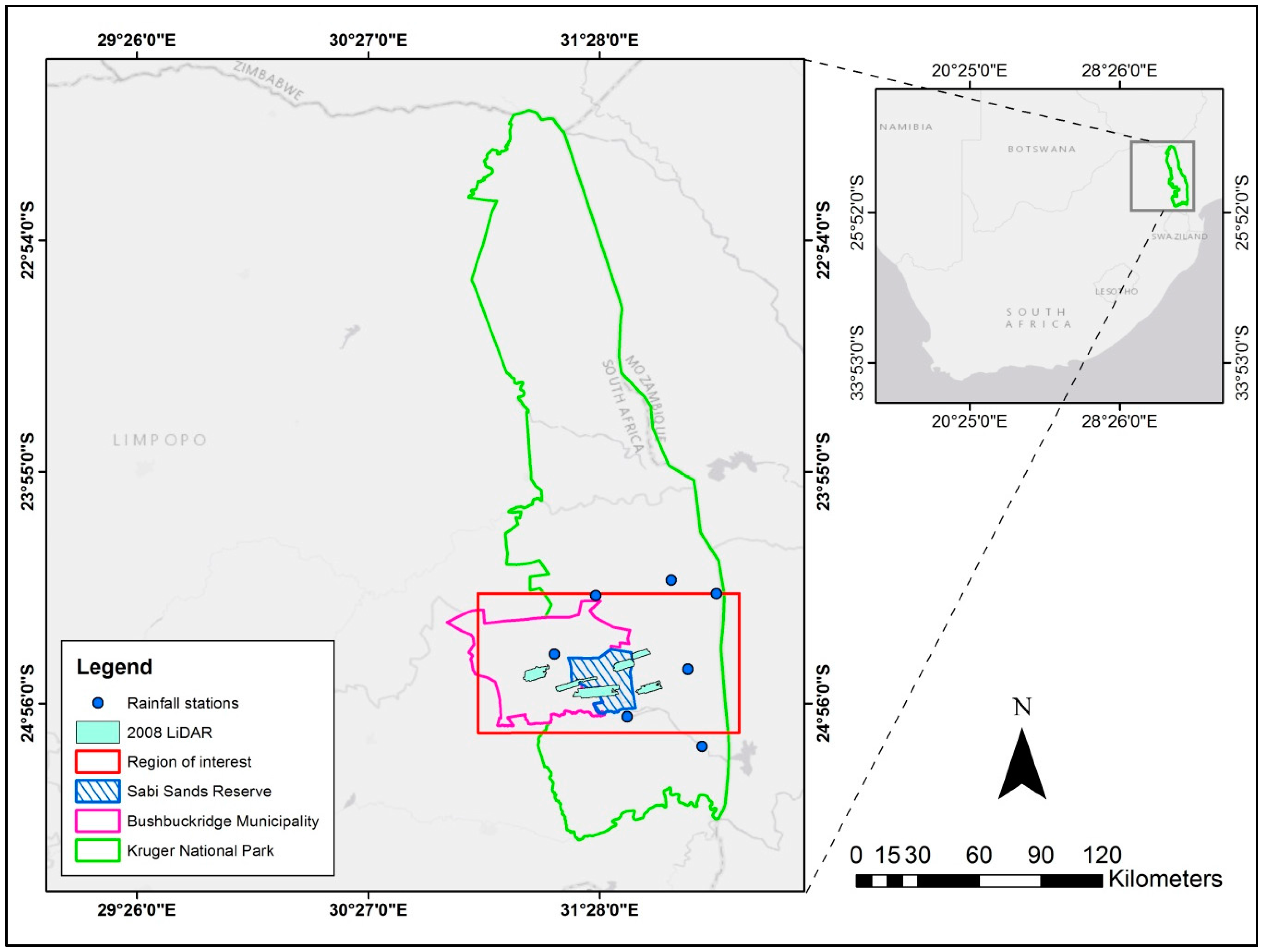
2. Study Area
3. Materials and Methods
3.1. Remote Sensing Data
3.2. Ancillary data
3.3. Sampling and Statistical Analysis
4. Results
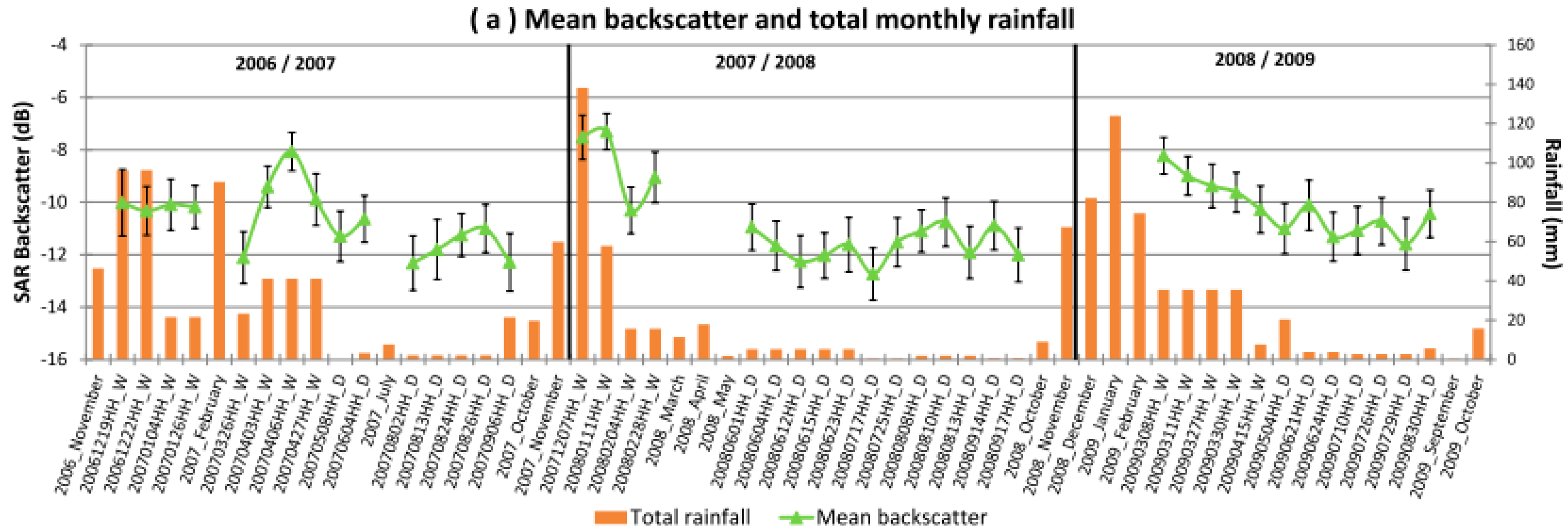
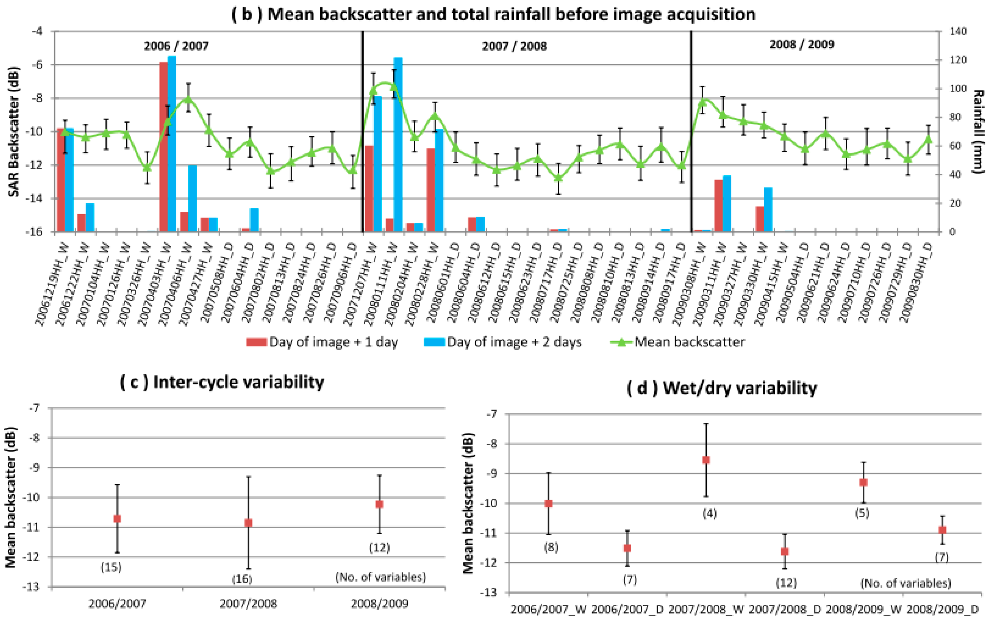
4.1. Rainfall Effects on Backscatter
4.2. Effects of Temporal Filter, Model, and Metric
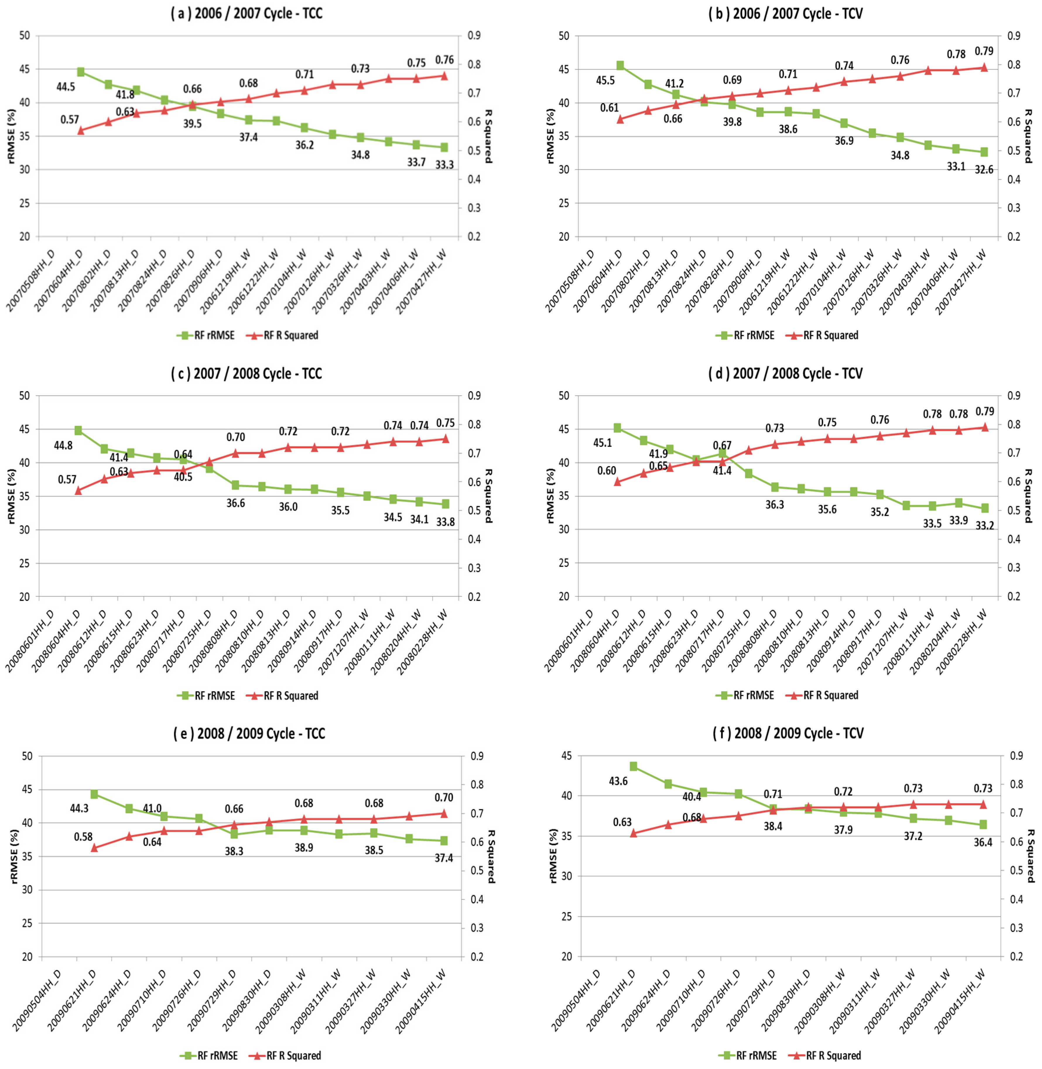
4.3. Wet and Dry Period Combinations
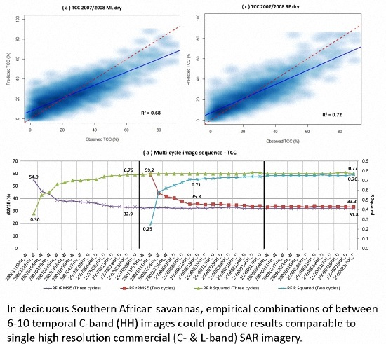
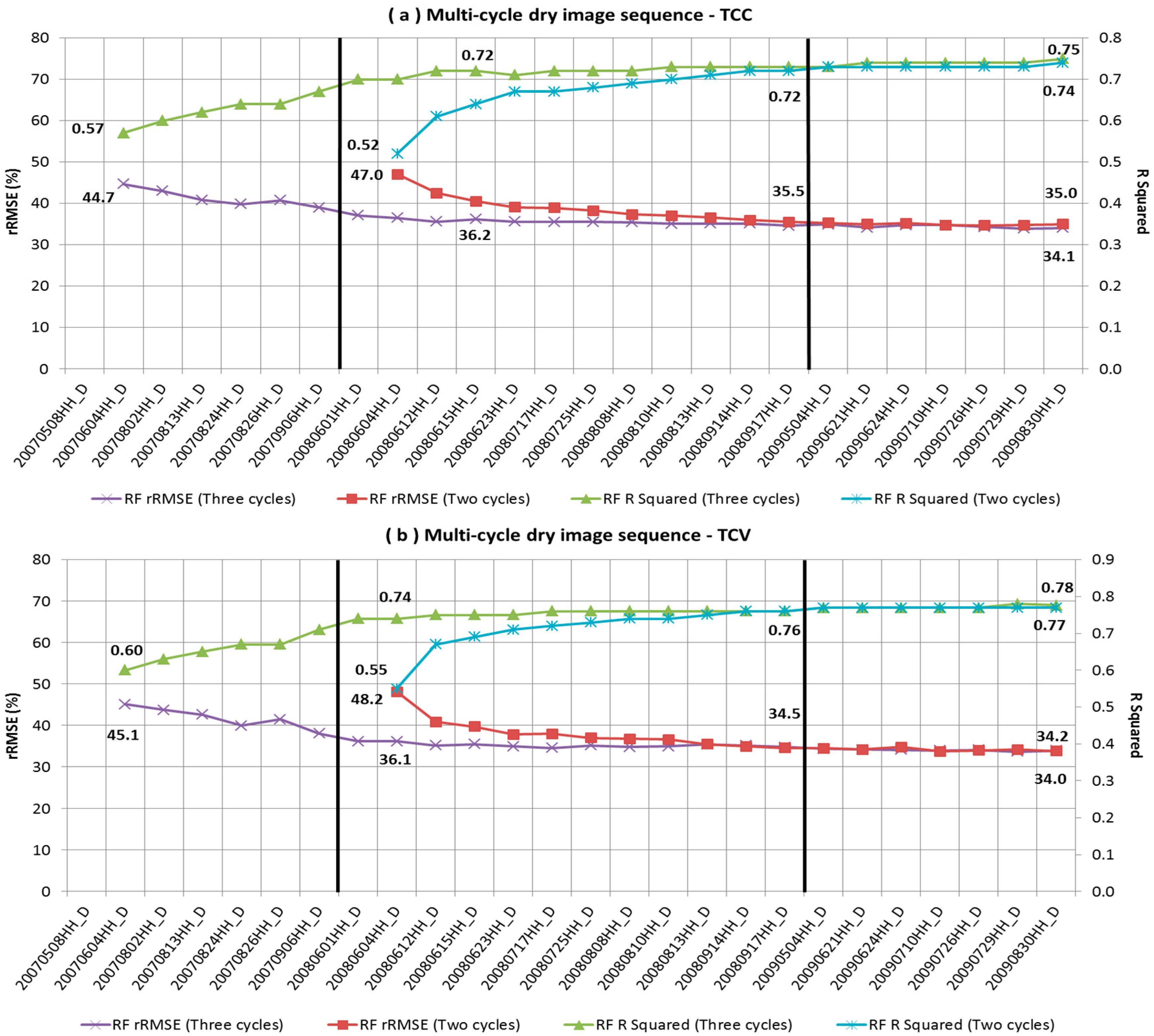
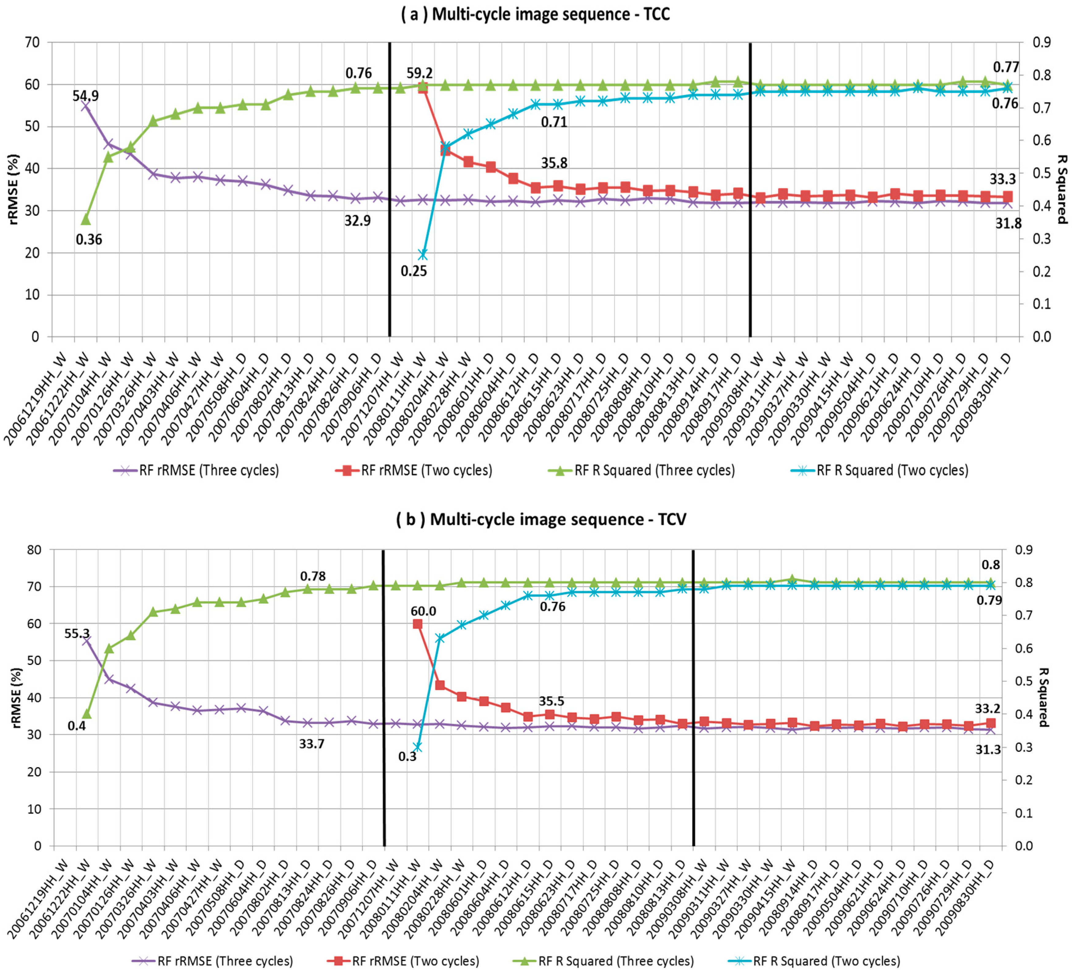
4.4. Image Sequences
5. Discussion
6. Conclusions
Acknowledgments
Author Contributions
Conflicts of Interest
References
- Scholes, R.J.; Archer, S.R. Tree-grass interactions in savannas. Ecology 2013, 28, 517–544. [Google Scholar]
- Sankaran, M.; Hanan, N.P.; Scholes, R.J.; Ratnam, J.; Augustine, D.J.; Cade, B.S.; Gignoux, J.; Higgins, S.I.; Le Roux, X.; Ludwig, F.; et al. Determinants of woody cover in African savannas. Nature 2005, 438, 846–849. [Google Scholar] [CrossRef] [PubMed]
- Twine, W.; Moshe, D.; Netshiluvhi, T.; Siphungu, V. Consumption and direct-use values of savanna bio-resources used by rural households in Mametja, a semiarid area of Limpopo province, South Africa. S. Afr. J. Sci. 2003, 99, 467–473. [Google Scholar]
- Shackleton, C.M.; Shackleton, S.E. The importance of non-timber forest products in rural livelihood security and as safety nets: A review of evidence from South Africa. S. Afr. J. Sci. 2004, 100, 658–664. [Google Scholar]
- Valentini, R.; Arneth, A.; Bombelli, A.; Castaldi, S.; Cazzolla Gatti, R.; Chevallier, F.; Ciais, P.; Grieco, E.; Hartmann, J.; Henry, M.; et al. A full greenhouse gases budget of Africa: Synthesis, uncertainties, and vulnerabilities. Biogeosciences 2014, 11, 381–407. [Google Scholar] [CrossRef] [Green Version]
- Matsika, R.; Erasmus, B.F.N.; Twine, W.C. A tale of two villages: Assessing the dynamics of fuelwood supply in communal landscapes in South Africa. Environ. Conserv. 2012, 40, 1–13. [Google Scholar] [CrossRef]
- Wigley, B.J.; Bond, W.J.; Hoffman, M.T. Bush encroachment under three contrasting land-use practices in a mesic South African savanna. Afr. J. Ecol. 2009, 47, 62–70. [Google Scholar] [CrossRef]
- Knapp, A.K.; Briggs, J.M.; Collins, S.L.; Archer, S.R.; Bret-harte, M.S.; Ewers, B.E.; Peters, D.P.; Young, D.R.; Shaver, G.R.; Pendall, E.; et al. Shrub encroachment in North American grasslands: Shifts in growth form dominance rapidly alters control of ecosystem carbon inputs. Glob. Chang. Biol. 2008, 14, 615–623. [Google Scholar] [CrossRef]
- Santos, J.R.; Lacruz, M.S.P.; Araujo, L.S.; Keil, M. Savanna and tropical rainforest biomass estimation and spatialization using JERS-1 data. Int. J. Remote Sens. 2002, 23, 1217–1229. [Google Scholar] [CrossRef]
- Mitchard, E.T.A.; Saatchi, S.S.; Lewis, S.; Feldpausch, T.R.; Woodhouse, I.H.; Sonké, B.; Rowland, C.; Meir, P. Measuring biomass changes due to woody encroachment and deforestation/degradation in a forest–savanna boundary region of central Africa using multi-temporal L-band radar backscatter. Remote Sens. Environ. 2011, 115, 2861–2873. [Google Scholar] [CrossRef]
- Dobson, M.C.; Ulaby, F.T.; Le Toan, T.; Beaudoin, A.; Kasischke, E.S.; Christensen, N. Dependance of radar backscatter on coniferous forest biomass. IEEE Trans. Geosci. Remote Sens. 1992, 30, 412–415. [Google Scholar] [CrossRef]
- Le Toan, T.; Beaudoin, A.; Riom, J.; Guyon, D. Relating forest biomass to SAR data. IEEE Trans. Geosci. Remote Sens. 1992, 30, 403–411. [Google Scholar] [CrossRef]
- Mitchard, E.T.A.; Saatchi, S.S.; White, L.; Abernethy, K.; Jeffery, K.; Lewis, S.L.; Collins, M.; Lefsky, M.A.; Leal, M.E.; Woodhouse, I.H.; et al. Mapping tropical forest biomass with radar and spaceborne LiDAR in Lopé National Park, Gabon: Overcoming problems of high biomass and persistent cloud. Biogeosciences 2012, 9, 179–191. [Google Scholar] [CrossRef]
- Lucas, R.M.; Cronin, N.; Lee, A.; Moghaddam, M.; Witte, C.; Tickle, P. Empirical relationships between AIRSAR backscatter and LiDAR-derived forest biomass, Queensland, Australia. Remote Sens. Environ. 2006, 100, 407–425. [Google Scholar] [CrossRef]
- Urbazaev, M.; Thiel, C.; Mathieu, R.; Naidoo, L.; Levick, S.R.; Smit, I.P.J.; Asner, G.P.; Schmullius, C. Assessment of the mapping of fractional woody cover in southern African savannas using multi-temporal and polarimetric ALOS PALSAR L-band images. Remote Sens. Environ. 2015, 166, 138–153. [Google Scholar] [CrossRef]
- Ningthoujam, R.; Balzter, H.; Tansey, K.; Morrison, K.; Johnson, S.; Gerard, F.; George, C.; Malhi, Y.; Burbidge, G.; Doody, S.; et al. Airborne S-band SAR for forest biophysical retrieval in temperate mixed forests of the UK. Remote Sens. 2016, 8, 609. [Google Scholar] [CrossRef]
- Lucas, R.M.; Moghaddam, M.; Cronin, N. Microwave scattering from mixed-species forests, Queensland, Australia. IEEE Trans. Geosci. Remote Sens. 2004, 42, 2142–2159. [Google Scholar] [CrossRef]
- Askne, J.; Santoro, M. Multitemporal repeat pass SAR interferometry of boreal forests. IEEE Trans. Geosci. Remote Sens. 2005, 43, 1219–1228. [Google Scholar] [CrossRef]
- Pulliainen, J.T.; Mikkela, P.J.; Hallikainen, M.T.; Ikonen, J.P. Seasonal dynamics of C-band backscatter of boreal forests with applications to biomass and soil moisture estimation. IEEE Trans. Geosci. Remote Sens. 1996, 34, 758–770. [Google Scholar] [CrossRef]
- Naidoo, L.; Mathieu, R.; Main, R.; Kleynhans, W.; Wessels, K.; Asner, G.P.; Leblon, B. Savannah woody structure modelling and mapping using multi-frequency (X-, C- and L-band) Synthetic Aperture Radar data. ISPRS J. Photogramm. Remote Sens. 2015, 105, 234–250. [Google Scholar] [CrossRef]
- Mathieu, R.; Naidoo, L.; Cho, M.A.; Leblon, B.; Main, R.; Wessels, K.; Asner, G.P.; Buckley, J.; van Aardt, J.A.N.; Erasmus, B.F.N.; et al. Toward structural assessment of semi-arid African savannahs and woodlands: The potential of multitemporal polarimetric RADARSAT-2 fine beam images. Remote Sens. Environ. 2013, 138, 1–17. [Google Scholar] [CrossRef]
- Wang, D.; Lin, H.; Chen, J.; Zhang, Y.; Zeng, Q. Application of multi-temporal ENVISAT ASAR data to agricultural area mapping in the Pearl River Delta. Int. J. Remote Sens. 2010, 31, 1555–1572. [Google Scholar] [CrossRef]
- Santoro, M.; Beer, C.; Cartus, O.; Schmullius, C.; Shvidenko, A.; McCallum, I.; Wegmüller, U.; Wiesmann, A. Retrieval of growing stock volume in boreal forest using hyper-temporal series of ENVISAT ASAR ScanSAR backscatter measurements. Remote Sens. Environ. 2011, 115, 490–507. [Google Scholar] [CrossRef]
- Pulliainen, J.T.; Kurvonen, L.; Hallikainen, M.T. Multitemporal behavior of L- and C-band SAR observations of boreal forests. IEEE Trans. Geosci. Remote Sens. 1999, 37, 927–937. [Google Scholar] [CrossRef]
- Askne, J.I.H.; Dammert, P.B.G.; Ulander, L.M.H.; Smith, G. C-band repeat-pass interferometric SAR observations of the forest. IEEE Trans. Geosci. Remote Sens. 1997, 35, 25–35. [Google Scholar] [CrossRef]
- Santoro, M.; Schmullius, C.; Pathe, C.; Schwilk, J.; Beer, C.; Thurner, M.; Fransson, J.E.S.; Shvidenko, A.; Schepaschenko, D.; McCallum, I.; et al. Estimates of forest growing stock volume of the northern hemisphere from ENVISAT ASAR. In Proceedings of ESA Living Planet Symposium, Edinburgh, UK, 9–13 September 2013; pp. 714–722.
- Townsend, P.A. Estimating forest structure in wetlands using multitemporal SAR. Remote Sens. Environ. 2002, 79, 288–304. [Google Scholar] [CrossRef]
- Kumar, S.; Pandey, U.; Kushwaha, S.P.; Chatterjee, R.S.; Bijker, W. Aboveground biomass estimation of tropical forest from Envisat advanced synthetic aperture radar data using modeling approach. J. Appl. Remote Sens. 2012, 6, 1–18. [Google Scholar] [CrossRef]
- Mucina, L.; Rutherford, M.C. (Eds.) The Vegetation of South Africa, Lesotho and Swaziland; South African National Biodiversity Institute: Pretoria, South Africa, 2006.
- Venter, K.J.; Scholes, R.J.; Eckhardt, H.C. The abiotic template and its associated vegetation pattern. In The Kruger Experience: Ecology and Management of Savanna Heterogeneity; Du Toit, J., Biggs, H., Rogers, K.H., Eds.; London Island Press: London, UK, 2003; pp. 83–129. [Google Scholar]
- GAMMA. Differential interferometry and geocoding software: DIFF&GEO. In GAMMA: Geocoding and Image Registration Documentation: User’s Guide; GAMMA: Gümligen, Switzerland, 2008. [Google Scholar]
- Quegan, S.; Yu, J.J. Filtering of multichannel SAR images. IEEE Trans. Geosci. Remote Sens. 2001, 39, 2373–2379. [Google Scholar] [CrossRef]
- Sheng, Y.; Xia, Z. A comprehensive evaluation of filters for radar speckle suppression. Int. Geosci. Remote Sens. Symp. 1996, 3, 1559–1561. [Google Scholar]
- Qiu, F.; Berglund, J.; Jensen, J.R.; Thakkar, P.; Ren, D. Speckle noise reduction in SAR imagery using a local adaptive median filter. GISci. Remote Sens. 2004, 41, 244–266. [Google Scholar] [CrossRef]
- Asner, G.P.; Knapp, D.E.; Kennedy-Bowdoin, T.; Jones, M.O.; Martin, R.E.; Boardman, J.; Field, C.B. Carnegie Airborne Observatory: In-flight fusion of hyperspectral imaging and waveform light detection and ranging for three-dimensional studies of ecosystems. J. Appl. Remote Sens. 2007, 1, 1–21. [Google Scholar] [CrossRef]
- Wessels, K.J.; Mathieu, R.; Erasmus, B.F.N.; Asner, G.P.; Smit, I.P.J.; van Aardt, J.A.N.; Main, R.; Fisher, J.; Marais, W.; Kennedy-Bowdoin, T.; et al. Impact of communal land use and conservation on woody vegetation structure in the Lowveld savannas of South Africa. For. Ecol. Manag. 2011, 261, 19–29. [Google Scholar] [CrossRef]
- Leckie, D.G.; Ranson, K.J. Forestry applications using imaging radar. In Principles & Applications of Imaging Radar. Manual of Remote Sensing; Henderson, F.M., Lewis, A.J., Eds.; John Wiley and Sons: Hoboken, NJ, USA, 1996; pp. 435–509. [Google Scholar]
- SAWS. South African Weather Service Rainfall Data 2006 to 2010; South African Weather Service: Pretoria, South Africa, 2015. [Google Scholar]
- SANParks. South African National Parks Rainfall Data 2006 to 2010; South African National Parks: Skukuza, South Africa, 2015. [Google Scholar]
- R Development Core Team. R: A Language and Environment for Statistical Computing; R Foundation for Statistical Computing: Vienna, Austria, 2016. [Google Scholar]
- Pickett, S.T.A.; Cadenasso, M.L.; Benning, T.L. Biotic and abiotic variability as key determinants of savanna heterogeneity at multiple spatio-temporal scales. In The Kruger Experience: Ecology and Management of Savanna Heterogeneity; du Toit, J.T., Biggs, H.C., Rogers, K.H., Eds.; Island Press: Washington, DC, USA, 2003; pp. 22–40. [Google Scholar]
- Breiman, L.; Friedman, J.; Stone, C.J.; Olshen, R.A. Classification and Regression Trees; The Wadsworth and Brooks-Cole Statistics-Probability Series; Taylor & Francis: Burlington, MA, USA, 1984. [Google Scholar]
- Naidoo, L.; Mathieu, R.; Main, R.; Kleynhans, W.; Wessels, K.; Asner, G.P.; Leblon, B. The assessment of data mining algorithms for modelling Savannah Woody cover using multi-frequency (X-, C- and L-band) synthetic aperture radar (SAR) datasets. IEEE Geosci. Remote Sens. Symp. 2014. [Google Scholar] [CrossRef]
- Wessels, K.J.; Colgan, M.S.; Erasmus, B.F.N.; Asner, G.P.; Twine, W.C.; Mathieu, R.; van Aardt, J.A.N.; Fisher, J.T.; Smit, I.P.J. Unsustainable fuelwood extraction from South African savannas. Environ. Res. Lett. 2013, 8, 1–10. [Google Scholar] [CrossRef]
- Chauhan, N.S.; Lang, R.H.; Ranson, K.J. Radar modeling of a boreal forest. IEEE Trans. Geosci. Remote Sens. 1991, 29, 627–638. [Google Scholar] [CrossRef]
- Bucini, G.; Hanan, N.P.; Boone, R.B.; Smit, I.P.J.; Saatchi, S.S.; Lefsky, M.A.; Asner, G.P. Woody fractional cover in Kruger National Park, South Africa. In Ecosystem Function in Savannas; CRC Press: Boca Raton, FL, USA, 2010; pp. 219–237. [Google Scholar]


| Phenological Cycle (October–September) | Total (mm) | Dry–Total (May–September) (mm) | Wet–Total (October–April) (mm) |
|---|---|---|---|
| 2006/2007 | 494.4 (111.2) | 107.3 (76.2) | 387.1 (146.2) |
| 2007/2008 | 432.8 (115.2) | 24.5 (105.3) | 408.4 (125.1) |
| 2008/2009 | 526.9 (119.7) | 52.4 (95.3) | 474.5 (144.2) |
| TCC | ||||||||||
|---|---|---|---|---|---|---|---|---|---|---|
| Speckle Suppression | Multi-Linear Regression | Random Forest | ||||||||
| Scenario | SISAmean | SISAStdev | R2 (CI) | RMSE (CI) | rRMSE (CI) | Bias | R2 (CI) | RMSE (CI) | rRMSE (CI) | Bias |
| Unfiltered | - | - | 0.6 (0.002) | 10.35 (0.043) | 43.09 (0.002) | 0.00 | 0.6 (0.003) | 10.36 (0.044) | 43.15 (0.002) | −0.05 |
| 3 × 3 Filter | 1 | 0.2 | 0.62 (0.003) | 10.05 (0.034) | 41.56 (0.002) | −0.01 | 0.64 (0.003) | 9.86 (0.034) | 40.75 (0.002) | −0.02 |
| 7 × 7 Filter | 0.99 | 0.27 | 0.66 (0.002) | 9.52 (0.028) | 39.63 (0.001) | 0.09 | 0.69 (0.003) | 9 (0.046) | 37.47 (0.002) | 0.05 |
| 11 × 11 Filter | 0.99 | 0.28 | 0.68 (0.003) | 9.24 (0.03) | 38.53 (0.001) | −0.01 | 0.72 (0.002) | 8.66 (0.032) | 36.1 (0.002) | −0.12 |
| TCV | ||||||||||
| Speckle Suppression | Multi-Linear Regression | Random Forest | ||||||||
| Scenario | SISAmean | SISAStdev | R2 (CI) | RMSE (CI) | rRMSE (CI) | Bias | R2 (CI) | RMSE (CI) | rRMSE (CI) | Bias |
| Unfiltered | - | - | 0.64 (0.004) | 22,806.7 (72.9) | 42.57 (0.002) | −29.88 | 0.64 (0.004) | 22,578.4 (88.1) | 42.14 (0.002) | −17.7 |
| 3 × 3 Filter | 1 | 0.2 | 0.66 (0.003) | 21,982 (85.5) | 40.62 (0.002) | 50.73 | 0.69 (0.003) | 21,210.6 (89.9) | 39.19 (0.002) | −120.3 |
| 7 × 7 Filter | 0.99 | 0.27 | 0.69 (0.003) | 20,981.9 (88.8) | 39.38 (0.002) | −159.01 | 0.74 (0.003) | 19,449.6 (108.8) | 36.5 (0.003) | −288.9 |
| 11 × 11 Filter | 0.99 | 0.28 | 0.71 (0.003) | 20,396.6 (81.5) | 38.42 (0.001) | 70.00 | 0.76 (0.003) | 18,710.1 (103.4) | 35.24 (0.002) | −97.8 |
| TCC | TCV | ||||||||
|---|---|---|---|---|---|---|---|---|---|
| R2 (CI) | RMSE (CI) | rRMSE (CI) | Bias | R2 (CI) | RMSE (CI) | rRMSE (CI) | Bias | Variables | |
| 2006/2007_W | 0.7 (0.004) | 8.92 (0.059) | 36.8 (0.003) | −0.06 | 0.74 (0.004) | 19,481.3 (102.9) | 36.41 (0.002) | −429.9 | 8 |
| 2006/2007_D | 0.67 (0.004) | 9.32 (0.045) | 38.72 (0.003) | 0.00 | 0.7 (0.004) | 20,813 (112) | 38.32 (0.002) | −10.8 | 7 |
| 2006/2007_WD | 0.76 (0.004) | 8.03 (0.052) | 33.32 (0.003) | −0.06 | 0.79 (0.003) | 17,578.9 (92.7) | 32.64 (0.002) | −262.6 | 15 |
| 2007/2008_W | 0.63 (0.004) | 9.99 (0.059) | 41.64 (0.003) | −0.03 | 0.67 (0.005) | 21,613.8 (152.7) | 40.37 (0.003) | −168.9 | 4 |
| 2007/2008_D | 0.72 (0.002) | 8.66 (0.032) | 36.1 (0.002) | −0.12 | 0.76 (0.003) | 18,710.1 (103.4) | 35.24 (0.002) | −97.8 | 12 |
| 2007/2008_WD | 0.75 (0.003) | 8.21 (0.047) | 33.79 (0.002) | −0.09 | 0.79 (0.003) | 17,533.8 (104.2) | 33.15 (0.002) | −229.7 | 16 |
| 2008/2009_W | 0.51 (0.005) | 11.5 (0.056) | 47.91 (0.003) | −0.13 | 0.57 (0.007) | 24,885.5 (178) | 46.19 (0.003) | −443.4 | 5 |
| 2008/2009_D | 0.67 (0.004) | 9.29 (0.044) | 38.4 (0.002) | −0.02 | 0.72 (0.004) | 20,110.7 (127.6) | 37.61 (0.002) | −26.8 | 7 |
| 2008/2009_WD | 0.7 (0.003) | 8.96 (0.037) | 37.35 (0.002) | 0.01 | 0.73 (0.004) | 19,566.9 (127.8) | 36.37 (0.002) | −143 | 12 |
| All Dry Images | 0.75 (0.004) | 8.22 (0.045) | 34.1 (0.002) | 0.01 | 0.78 (0.003) | 17,942.7 (112.2) | 33.96 (0.002) | −22.5 | 26 |
| All Images | 0.77 (0.003) | 7.78 (0.053) | 31.77 (0.002) | −0.19 | 0.8 (0.003) | 16,846.5 (95.3) | 31.31 (0.002) | −267.4 | 43 |
© 2016 by the authors; licensee MDPI, Basel, Switzerland. This article is an open access article distributed under the terms and conditions of the Creative Commons Attribution (CC-BY) license (http://creativecommons.org/licenses/by/4.0/).
Share and Cite
Main, R.; Mathieu, R.; Kleynhans, W.; Wessels, K.; Naidoo, L.; Asner, G.P. Hyper-Temporal C-Band SAR for Baseline Woody Structural Assessments in Deciduous Savannas. Remote Sens. 2016, 8, 661. https://0-doi-org.brum.beds.ac.uk/10.3390/rs8080661
Main R, Mathieu R, Kleynhans W, Wessels K, Naidoo L, Asner GP. Hyper-Temporal C-Band SAR for Baseline Woody Structural Assessments in Deciduous Savannas. Remote Sensing. 2016; 8(8):661. https://0-doi-org.brum.beds.ac.uk/10.3390/rs8080661
Chicago/Turabian StyleMain, Russell, Renaud Mathieu, Waldo Kleynhans, Konrad Wessels, Laven Naidoo, and Gregory P. Asner. 2016. "Hyper-Temporal C-Band SAR for Baseline Woody Structural Assessments in Deciduous Savannas" Remote Sensing 8, no. 8: 661. https://0-doi-org.brum.beds.ac.uk/10.3390/rs8080661