Analyzing Landscape Trends on Agriculture, Introduced Exotic Grasslands and Riparian Ecosystems in Arid Regions of Mexico

Abstract

Riparian Zones are considered biodiversity and ecosystem services hotspots. In arid environments, these ecosystems represent key habitats, since water availability makes them unique in terms of fauna, flora and ecological processes. Simple yet powerful remote sensing techniques were used to assess how spatial and temporal land cover dynamics, and water depth reflect distribution of key land cover types in riparian areas. Our study area includes the San Miguel and Zanjon rivers in Northwest Mexico. We used a supervised classification and regression tree (CART) algorithm to produce thematic classifications (with accuracies higher than 78%) for 1993, 2002 and 2011 using Landsat TM scenes. Our results suggest a decline in agriculture (32.5% area decrease) and cultivated grasslands (21.1% area decrease) from 1993 to 2011 in the study area. We found constant fluctuation between adjacent land cover classes and riparian habitat. We also found that water depth restricts Riparian Vegetation distribution but not agricultural lands or induced grasslands. Using remote sensing combined with spatial analysis, we were able to reach a better understanding of how riparian habitats are being modified in arid environments and how they have changed through time.

1. Introduction

Riparian ecosystems (RE) are considered critical environments, due to the goods and services they provide, for established and developing human populations around the world [1,2]. Described as transition zones between aquatic and terrestrial environments, with high fluxes of material, water and energy [3,4,5], RE are often considered biodiversity hotspots [6,7] as well as ecosystem services hotspots [3,8,9,10,11,12]. However, human activities such as livestock ranching, agricultural development and urbanization could result in the modification and degradation of these systems, diminishing their capacity to sustain their ecological function and thus provide services in the future.

Only 0.1% to 0.5% of the surface covered by arid environments in northwestern Mexico and the Southwestern US are RE [5,13,14]. Despite this, RE represent key habitats in arid environments, since the availability of water makes them unique in terms of their fauna, flora and ecological processes [15]. However, since economic and human activities are highly dependent on the availability and quality of water, the RE in arid environments are often subject to high rates of change and modification [15,16].

Due to the accessibility of freshwater, two of the most common activities associated with riparian systems in arid lands are agriculture (crop yielding) and livestock ranching [17,18]. Since these activities typically modify the systems where they occur, it is critical to monitor how much of the riparian habitat is used by them, as well as analyze the effects that these activities are having on the health and presence of riparian zones.

The San Miguel and the Zanjon Rivers (SMR and ZR), two sub-watersheds in arid Northwestern Mexico, have experienced RE modification. Native riparian vegetation has been replaced by extensive cultivations of exotic grasslands for cattle foraging [19,20,21,22] in the watershed and the establishment of agricultural fields on the side of riverbeds [23]. The alterations of these landscapes has been ongoing for over 300 years [24]. However, starting in the 1950s, the introduction of exotic species for forage, a boom in agriculture (both in area used and intensity of usage) and a subsequent increase in water extraction (usually by wells), have altered the landscape with greater intensity [23,25,26].

In this study, we conducted a historical analysis on the transitions between vegetation types on two sub-watersheds in arid Northwestern Mexico. Using the approach proposed in this paper, historical as well as contemporary land cover distribution maps of riparian vegetation were generated.

Addressing Landscape Dynamics on Riparian Vegetation

Land cover changes of riparian systems in the Southwestern US and Northwestern Mexico have been occurring constantly over the last centuries [14,17,27,28,29,30]. However, the monitoring of land cover change over extensive areas was extremely challenging and resource consuming until technological capabilities provided by remote sensing approaches were developed [15,31]. In this study, we use land cover classification algorithms [32,33], coupled with post-classification change detection techniques [34,35], to map the magnitude and location of land cover change over two sub-watersheds in arid Northwestern Mexico. We also used spatial analysis techniques to determine water depth under the riverbed [36] and the previously generated land cover thematic maps to account for the effect of water depth on riparian vegetation and other key land cover types.

Our focus in the present work was to assess the transitions within the riparian, agricultural and grassland cover classes in our study area between 1993 and 2011, as well as examine the relationship between these land cover types and water depth. Our objectives were: (1) to quantify land cover changes on riparian zones in arid environments; and (2) to observe if land cover distributions are related to water depth, which is often modified by ground water pumping for agricultural purposes.

2. Materials and Methods

We utilized Landsat Thematic Mapper (TM) image data to generate thematic classification maps (for 1993, 2002 and 2011), followed by an accuracy assessment for each of the products generated. After this, a land cover change assessment was performed, to assess the primary conversions that occurred for: (1) the entire river basin; and (2) the main riparian corridor. Emphasis was paid to changes due to agricultural activities or other environmental conditions (such as ground water). Finally, we generated continuous surfaces of water depth on the river in order to analyze how this variable relates to the dynamics of key land cover types on the area influenced by the river.

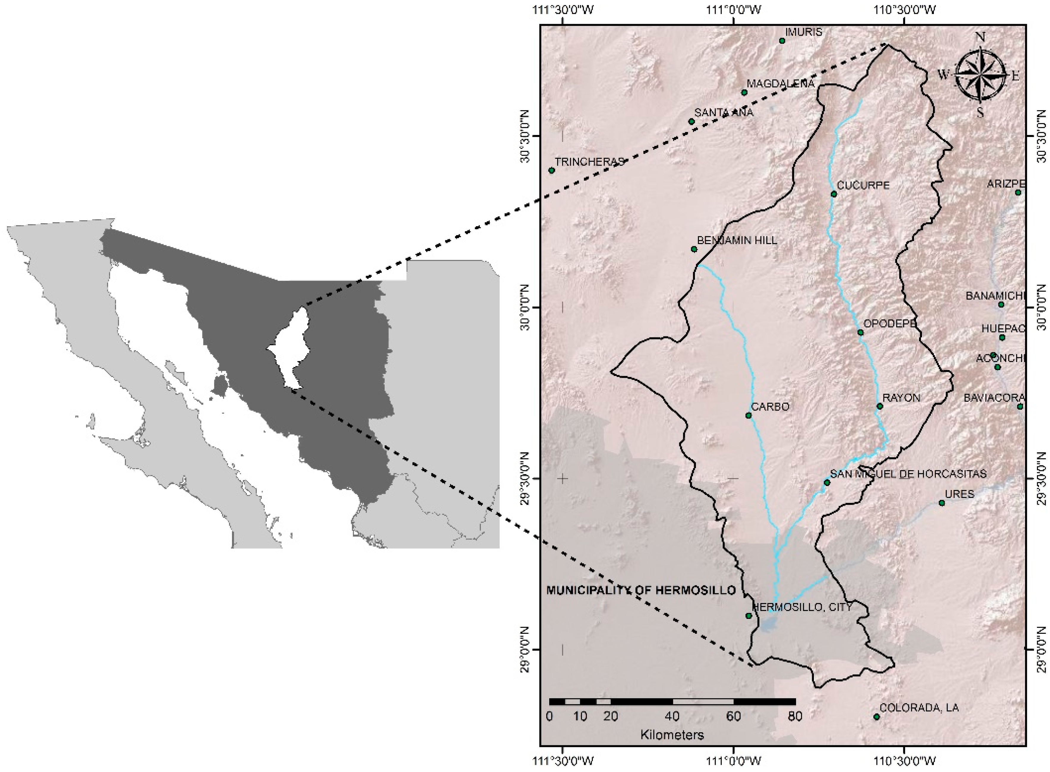
2.1. Study Area

The study area is composed of the SMR and the ZR, two sub-watersheds of the Sonora watershed in Northwestern Mexico. The riparian systems are located northeast of the city of Hermosillo, between the coordinates 28°53′N–30°46′N latitude and 110°21.5′W–111°21.5′W longitude (Figure 1). The approximate extent of the study area is 9437 km² (around 30% of the entire area of the Sonoran watershed), and elevation above sea level ranges from approximately 200 m to 2000 m (at Sierra Azul). In this region, potential annual evapotranspiration is 2400 mm, the mean annual temperature is 21 °C and the mean annual precipitation is about 421 mm, with 70% of it occurring during the summer (June–August) monsoon [37]. The ZR is cataloged as an ephemeral river, while the SMR has both ephemeral (in most of its extension) and perennial flow segments between Cucurpe and Fabrica de los Angeles. It is in one of these perennial segments on the SMR, where the hydrometric station “El Cajon” has measured water flow since 1974 [38]. The mean annual runoff measured in this hydrometric station is 32.33 mm³. Since 1996, a decrease in water flow has been observed and in 2012 the annual runoff was 8.174 mm³ [39]. Information regarding geological parameters on the watershed can be found elsewhere [40].

According to Shreve and Wiggins (1964) [41], the SMR falls within the Arizona Uplands and the ZR is part of the Sonoran Desert Plains. The National Forest Inventory (NFI) lists Subtropical Scrub, Forest and Mesquite as the most dominate vegetation cover types in the SMR. Grasslands and Desert Scrubs are the most prominent covers in the ZR sub-watershed [42].

During the last three centuries, the main economic activities in the SMR and ZR sub-watersheds have been agriculture and cattle ranching [37,43]. Cattle ranching activities became more intensive in both sub-watersheds in the 1950s when buffelgrass (Cenchrus ciliaris) was introduced [22]. The presence of buffelgrass pastures in both areas represents a significant pressure on the river system, since pastures have been established in areas adjacent to the riparian habitats. Buffelgrass has been documented, in the Sonoran Desert, to outcompete and displace native flora by invading adjacent areas where it was not planted [20,21,22].

Another factor impacting the area is the water provisioned to the city of Hermosillo (more than 800,000 habitants), especially due to the construction of the Abelardo L. Rodriguez dam and the drilling of wells to extract water for urban and agricultural use [23].

2.2. Datasets and Variables Processed

2.2.1. Image Classification and Change Detection

We chose to use Landsat TM image data because: (1) they provide an extensive historical record for most places on Earth; and (2) the sensor’s proven capabilities regarding its use in land cover detection and change studies in arid and semiarid riparian systems [15,31]. For this study, we conducted our analysis at intervals of approximately ten years (1993, 2002 and 2011) to analyze changes in riparian vegetation and areas associated with either agriculture (croplands) or cattle ranching. To generate each classification two Landsat TM images were used per year, one prior to and one post monsoon (summer rain), to leverage the phenological characteristics of vegetation as a classification element [15,44]. Our study area is covered by two Landsat TM Scenes (Path 35-Row 39 and Path 35-Row 40) with the collection dates varying from year to year (

Table 1. Dates of the Landsat TM Scenes selected by year.

Year	Pre-Monsoon Date	Post-Monsoon Date
1993	10 April	17 September
2002	21 May	25 August
2011	28 April	19 September

). The images were obtained from the Earth Explorer platform, managed by the United States Geological Survey [45].

The Landsat TM Surface Reflectance images (CDR) acquired were orthorectified and processed through the Landsat Ecosystem Disturbance Adaptive Processing System (LEDAPS) to reduce atmospheric noise [45,46,47]. A 30-m resolution Digital Elevation Model (DEM) was acquired from the National Elevation Dataset archives maintained by the US geological Survey [45]. To improve the quality of the DEM, we resampled it to correct for sinks and tops [36].

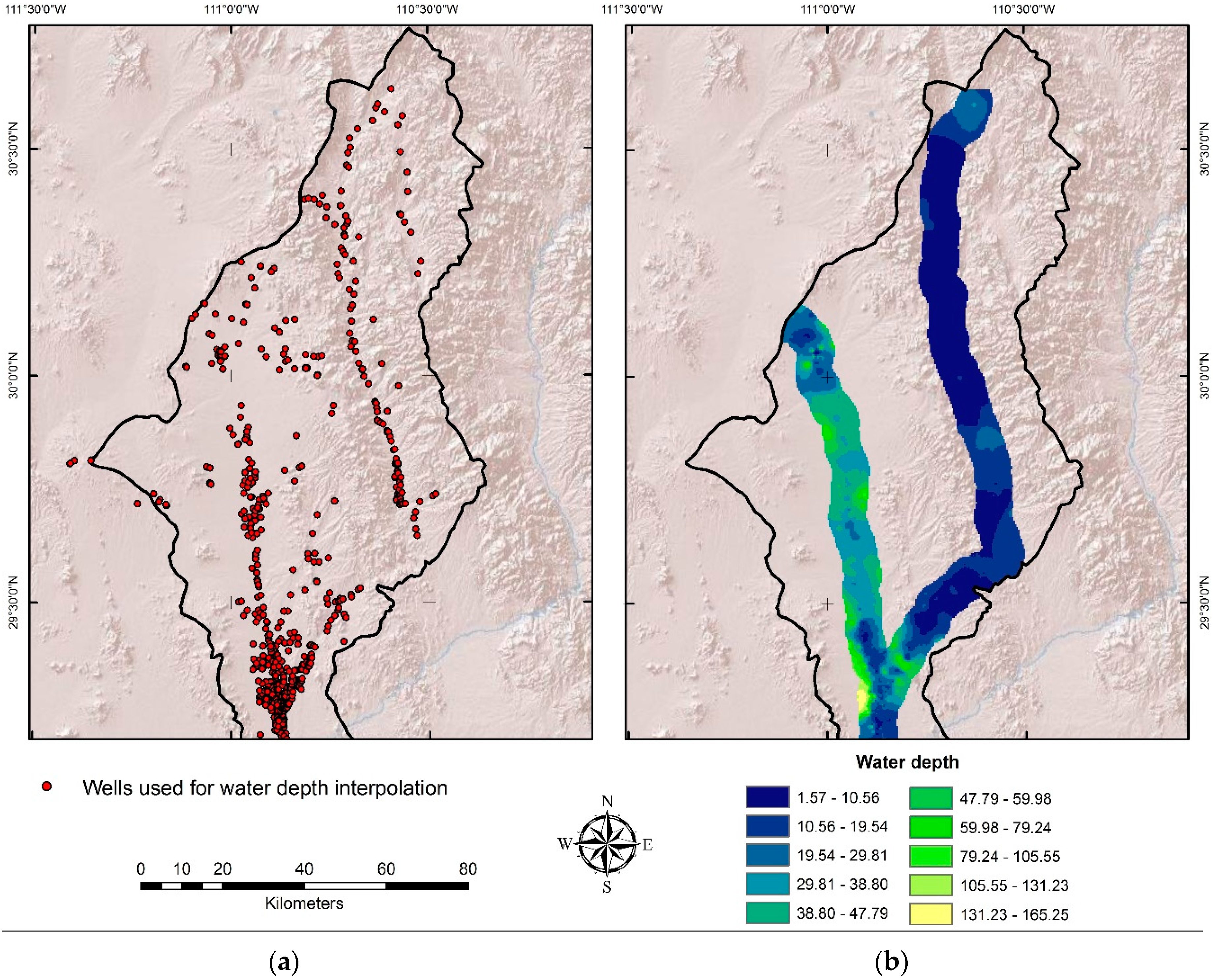
2.2.2. Development of Water Depth Surfaces

Ground water depth data were acquired from the regional ground water office of the National Water Commission (CONAGUA). We obtained the location and water static levels, collected between 2005 and 2013, for 665 wells (212 in the SMR and 453 in the ZR). We obtained readings for static water level in each well with various frequencies (from once a year to once every three years). Since water levels were tested around the same time each year, we proceeded to average the readings in order to obtain a representation of water depth per well in the study area for the period between 2005 and 2013.

2.3. Classification and Change Detection

2.3.1. Classification Scheme

To develop our classification scheme (

Table 2. Description of the types of land use–land cover used for the classification scheme.

ID	Class	Code	Description
1	Agriculture	AG	Areas of perennial crops such as grapes, walnuts and oranges or annual crops including vegetables.
2	Water	W	Areas of permanent water with total cover more than 30 m in length.
3	Bare Soil	BS	Areas of rock, barren soil or less than 10% vegetation cover. Represents mainly mining areas, some rural roads, waterways and highly impacted areas.
4	Desert Scrub	DS	Areas of small-leaved shrubs that grow on alluvial soils that may include groups of thorny species. Within this class can be found species belonging to the genera Cercidium (Parkinsonia), Olneya, Condalia, Lycium, Opuntia and Fouquieria, among others.
5	Mesquite Woodland	MW	Areas principally dominated by Prosopis and other subtropical or thorny trees.
6	Grassland Cultivated/Induced	GCI	Areas of buffelgrass introduced by direct seeding.
7	Riparian Vegetation (include Riparian Mesquite)	RV	Areas of woody vegetation located on the banks of the riverbed. They are characterized by the presence of species that require favorable moisture conditions such as Populus sp. This class may present individuals of the gennus Prosopis.
8	Subtropical/Succulent Scrub	SS	Areas of vegetation mainly formed by shrubs or low, thorny trees. They are described as an ecological transition between the class of forest and thorny scrub. The main genera that can be observed are Ipomoea, Bursera and Acacia, to name a few. In regions of hills and middle elevations, Cercidium microphyllum, Opuntia sp., Carnegia gigantea and Lophocereus schottii are the dominant species.
9	Forest (Oak and Oak/Pine)	F	Areas of woody vegetation found in temperate or cold climates with higher humidity. The canopy cover of this class is observed in more than 10% of the area with heights up to 15 m high.
10	Natural/Native Grassland	GN	Areas dominated by native grasses. Located mainly in the areas of transition between Forest-Subtropical Shrub and forest-Desert Scrub.

) featuring the classes of interest for our analysis, we utilized a combined methodology. First, we used a method proposed by Anderson et al. (1976) [48] where land cover classes were described generally (Level 1 classes, e.g., water, scrub, forest, etc.) according to the capabilities of Landsat TM like sensors. In order to achieve greater detail in our classification, we made further subdivisions of classes using a classification scheme proposed by the Mexican National Forest Commission (CONAFOR) where they describe plant communities according to their physiognomic, floristic and ecologic characteristics [42]. The class denoted as “Urban Area” was inserted after the automated classification was performed using aerial photos and historical datasets as a reference. This was done due to misclassification and the “Urban Area” being rather small.

2.3.2. Classification Model

There are multiple classification techniques available to create maps regarding land cover for a set of properly pre-processed remotely sensed datasets [34,35,49,50]. We used a Classification and Regression Tree (CART) model approach to generate the land cover maps for our study [51,52,53]. CART models have been shown to be accurate when classifying landscape imagery [54,55] and better than other techniques when classifying arid environments [15,44]. Using a CART model, we generated land cover maps for each year of the study using the variables derived from the two Landsat TM images collected and the DEM (

Table 3. Variables used in the land cover classification derived from Landsat spectral reflectance data and a Digital Elevation Model (DEM).

Variable	Reference	No. of Layers	Description
Normalized Difference Vegetation Index (NDVI)	[56]	2	The reflectance properties of vegetation (in the red and near infrared) are used to derive a productivity proxy [33,56,57]
Soil Adjusted Vegetation Index (SAVI)	[58]	2	Minimizes the effect of soil reflectance on the quality of information generated by incorporating a correction factor in the denominator of the classical equation of NDVI [58].
Enhanced Vegetation Index	[59,60]	2	Optimizes the vegetation signal increasing its sensitivity in regions of high biomass and reducing atmospheric interference. These characteristics are used to help reduce the possible saturation of data that can be present with the NDVI [60].
Reflectance	Landsat TM	12	Represented as a percentage. Obtained by dividing the energy reflected by a material in a certain wavelength by the incident energy [32].
Tasseled Cap	[61]	12	Displays data that defines vegetation cover. Provides information on greenness, wetness and brightness of each pixel in the image [32].
Multitemporal Kauth–Thomas (MKT)	[62]	12	Provides vegetation dynamics between two images using their reflectance. The analysis requires a layer stack containing the bands of the two scenes acquired for the same year.
Principal Components	[62]	12	A statistical technique applied to remotely sensed data used to find the causes of variability in an image and sort these causes in order of importance [32].
Texture	[63]	12	In this case the texture refers to a description of the spatial variability of tones found within a scene [32].
Elevation, Aspect and Slope	USGS (NED)	3	Represents the topographic conditions of the area which are derived from the Digital Elevation Model (DEM).

).

The supervised classification approach requires that the user extract variables from layers of spatial information (scenes of Landsat TM) and auxiliary information (DEM) as a prerequisite for obtaining thematic maps of land use [15,32]. The set of derived variables and the DEM were rescaled and re-projected in order to generate a satisfactory and consistent vertical integration [35]. A layer stack was generated resulting in a single image per year (1993, 2002 and 2011) for each Landsat scene (Path 35-Row 39 and Path 35-Row 40) containing all the information generated for a total of 69 layers per year. Finally, the stacks were clipped to the area of interest.

Using the “clipped variable stack”, we proceeded to collect training points for each of the classes listed in our class scheme (Table 2) to run the classification models.

2.3.3. Supervised Classification and Accuracy Assessment

Training datasets for each of the land cover types were generated [32]. To do this, we collected samples: (1) in the field for each land cover class in the study area (collected during a field season in the study area); (2) using historical aerial photography provided by web services; and (3) from the Landsat imagery (only when the land cover was obvious, as in the case of water bodies or agriculture parcels). We collected between 60 and 150 samples per class in order to train our classification model.

After the training points were fed in to the classification model and the thematic classification maps were created, we used a confusion matrix to assess the accuracy of each classification map produced [34,64,65]. To create the confusion matrices, we applied a stratified random sampling of 30 points per class over each classified thematic map (with the exception of water and bare soil classes where we used 15 points per class) and assessed the accuracy of the classification by comparing the map to reality (assessed with field visits and high spatial resolution aerial imagery). Finally, we obtained statistical measurements from the confusion matrix such as: (1) producer’s and user’s accuracy; (2) overall accuracy; and (3) the Kappa statistic [65].

2.3.4. Change Detection in the Watershed and along the Rivers

After joining the two sections of the watershed (the north and the south portions) to create a single classification, for each of the years covered in this study, we proceeded to perform a change detection analysis [66]. Specifically, we used the thematic classifications to generate a post-classification change detection analysis [15,44] between: (1) 1993 and 2002; (2) 2002 and 2011; and (3) 1993 and 2011. Through this analysis we address changes on a 5 km buffer from the two main water streams present in the watershed (the SMR and ZR). Our main interest was to address total change produced by human activities as a main driver for land cover change.

2.4. Water Depth

To generate continuous surfaces regarding ground water depth, we used the Inverse Distance Weighting (IDW) interpolation approach [36]. This method measures the weighted average between known measurements between nearby points giving the greatest weight to the nearest point [36]. We considered this method to be optimal for our study area since well density in the riparian areas is high and the distance between wells is small. The following function describes the IDW:

$$Z\mathit{\left(}\mathrm{x}\mathit{\right)}\text{=}{\displaystyle \mathit{\sum }}_{\mathrm{i}}{\omega }_{\mathrm{i}}{z}_{\mathrm{i}}/{\displaystyle \mathit{\sum }}_{\mathrm{i}}{\omega }_{\mathrm{i}}$$

$${\omega }_{\mathrm{i}}\text{= 1/}{{\mathrm{d}}_{\mathrm{i}}}^2$$

where Z(x) is the unknown value to be interpolated in x; Z_i is the known value; d_i is the distance; and ω_i is the pondered value (Inverse square of the distance).

We specified a 30-m spatial resolution for the output to allow direct comparison to the Landsat TM classification and change detection outcomes. The continuous water depth surface was measured in meters. Since we did not obtain reliable piezometric level measurements for the southernmost portion of the watershed our datasets only cover from a latitude of 29°12′00″ to the north.

2.5. Relationships between Water Depth and Land Cover along the River

Using a 5 km buffer around the main water stream present in both sub-watersheds, we analyzed how water depth relates to land cover distribution and change in the riparian areas. As a sampling approach we selected 20 polygons (larger than 3 Ha to obtain at least 33 pixels in each area), distributed throughout the watershed, for areas where Riparian Vegetation, Agriculture and Grassland Cultivated/Induced did not change between 2002 and 2011. We extracted another 40 polygons where Riparian Vegetation was present in 2002 (20 with water depth lower than 10 m and 20 where water depth was greater than or equal to 10 m). Finally, we conducted an analysis on these polygons comparing the water depth: (1) with the land cover types (using a simple ANOVA); and (2) changes in Riparian Vegetation.

3. Results and Discussion

3.1. Classification Accuracy

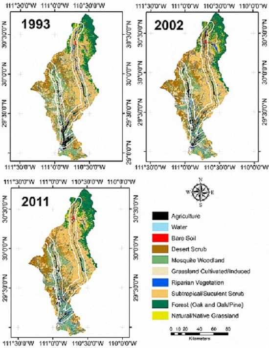
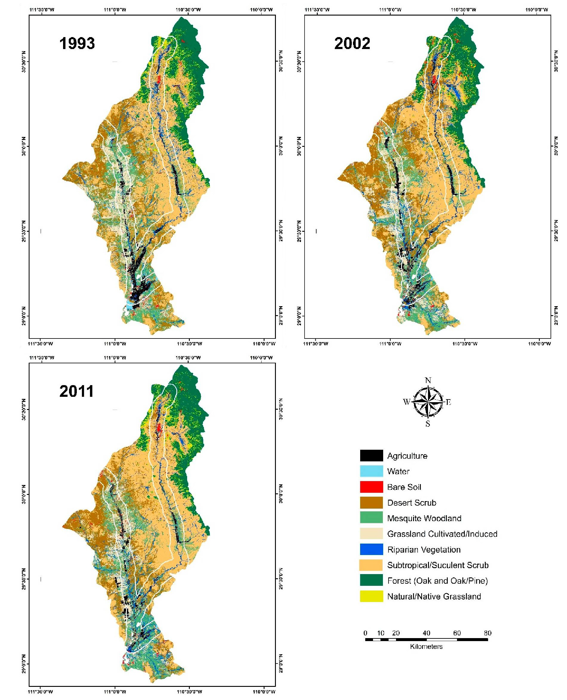
The overall accuracies for our classifications were greater than 78% for the three maps generated (

Table 4. Summary of the User’s, Producer’s, Kappa and Overall accuracies for the CART (Classification and regression Tree) based vegetation classifications for 1993, 2002 and 2011.

Class	1993		2002		2011
	User’s Accuracy %	Producer’s Accuracy %	User’s Accuracy %	Producer’s Accuracy %	User’s Accuracy %	Producer’s Accuracy %
Agriculture	95	86	85	89	80	94
Water	100	100	100	100	100	100
Bare Soil	60	75	60	75	70	100
Desert Scrub	70	52	80	59	75	75
Mesquite Woodland	85	65	75	65	80	53
Grasslands Cultivated/Induced	60	86	80	94	75	79
Riparian Vegetation (includes Riparian Mesquite)	70	100	80	100	80	100
Subtropical/Succulent Scrub	85	71	80	73	90	69
Forest (Oak and Oak/Pine)	90	90	85	94	85	94
Natural/Native Grassland	75	100	80	80	75	88
Overall accuracy %	78.9		80.6		80.6
Kappa coefficient	0.764		0.783		0.783

, Figure 2). User’s accuracy values ranged from 60% to 100% and producer’s accuracy values ranged from 52% to 100%. These results fall within the acceptable range for accuracy [67] and the errors present are likely due to the spectral similarities of certain classes.

Bare Soil was often confused with the Mesquite Woodland and Grasslands classes due to very low vegetation density in the desert leading to almost nonexistent vegetation reflectance. In addition, the Grasslands class was often confused with classes like Desert Scrub and Mesquite Woodland since the class often contained elements of those two types of vegetation as part of its structure. Most of the land cover classes were correctly classified for our three maps (Figure 3) this is likely due to their: (1) Unique reflectance characteristics; (2) Particular phenological cycles; and (3) Presence in areas with distinctive topographical characteristics (slope, aspect or elevation). The two classes that obtained the highest accuracies were the Forest (Oak and Oak/Pine) and Water classes. This was expected since these two types of features have unique characteristics.

3.2. Trends and Changes in the Riparian Areas (1993–2011)

Using the classification outputs and the 5 km buffer around the SMR and ZR, we calculated two statistics: (1) Total change per class through time; and (2) The change among classes through time focusing on the Agriculture, Riparian Vegetation and Grasslands classes [15,44].

3.2.1. Land Cover Trends along the Rivers

We proceeded to analyze the trends for the 5 km buffer around the SMR and ZR using the classified land cover maps (

Table 5. Land cover trends for the 5 km buffer in the ZR and SMR sub-watersheds.

Class Name	Area Ha 1993	Area Ha 2002	Area Ha 2011	Change Ha (1993–2011)	% Change (1993–2011)
Agriculture	21,883	21,231	14,763	−7120	−32.5
Water	964	60	62	−902	−93.6
Bare Soil	2845	3337	4134	1289	45.3
Desert Scrub	30,452	41,247	34,936	4484	14.7
Mesquite Woodland	49,039	49,151	50,745	1706	3.5
Grassland Cultivated/Induced	43,089	37,880	34,004	−9085	−21.1
Riparian Vegetation	22,176	22,567	22,801	625	2.8
Subtropical/Succulent Scrub	79,646	75,146	87,779	8133	10.2
Forest (Oak and Oak/Pine)	5823	6851	7922	2099	36.0
Natural/Native Grassland	4884	3332	3658	−1226	−25.1

). We observed a general decrease in the Agriculture and Grasslands classes and a significant increase in the extent of the Subtropical and Desert Scrub classes. We also observed very little change in the Riparian Vegetation areas (Table 5).

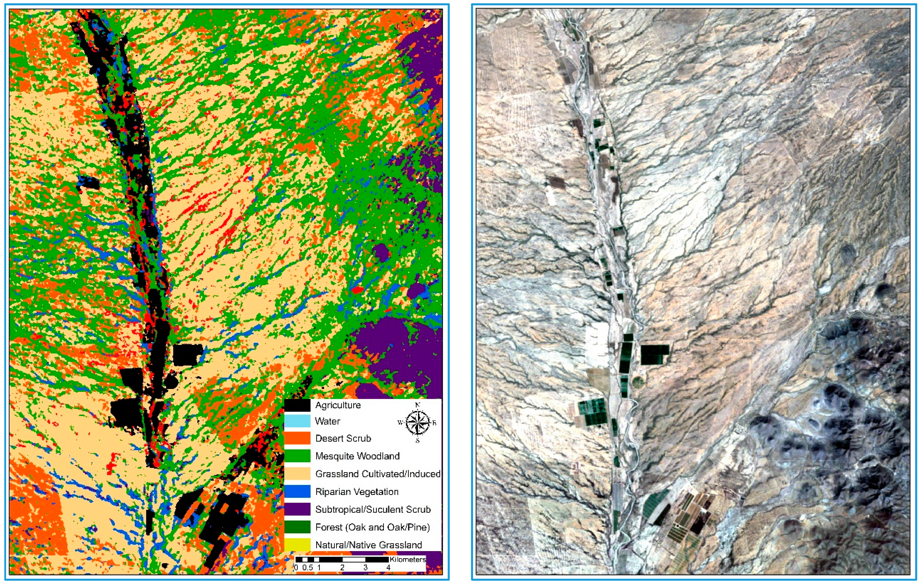
Human activities have caused a drastic change in land cover throughout the SMR and ZR sub-watersheds. Some of the most important changes are related to the establishment and abandonment of agricultural fields (vineyards, pecan orchards, pastures and others), the cultivation of buffelgrass pastures and extensive cattle ranching activities [20,68]. It is important to mention that changes in the area might be related to other factors such as climatic trends, species competition and water redistribution [68,69].

The previous results suggest two important trends. First, the extent of area used as agricultural land near the river has been decreasing. This is consistent with data suggesting that water is now being used for urban use rather than for agricultural purposes [68]. This has led to restrictions on water for agriculture and the abandonment of activities along both rivers. Second, the observed decrease in area indicates that induced grasslands used as pastures are not as resilient or pervasive as suggested previously [20,21,22]. This was expected since the maintenance of the pastures is often intensive [37] and the governmental programs that introduced them are no longer providing the means to implement more grasslands or maintain the current pastures [70].

3.2.2. Changes in Induced Grasslands, Agriculture and Riparian Vegetation in the SMR-ZR (1993–2011)

Using the land cover change maps derived for 1993–2011 and the 5 km buffer for our riparian zone, we were able to analyze how and where Agriculture, Induced Grasslands and Riparian Vegetation changed in our study area.

Riparian Vegetation

Our results show that Riparian Vegetation is more prone to change than Subtropical/Succulent Scrub, Mesquite Woodland or Agriculture even though these classes most often converted to Riparian Vegetation (

Table 6. Land cover trends relative to the Riparian Vegetation class along the 5 km buffer in both sub-watersheds.

From	To	1993–2011 Ha
Riparian Vegetation	Agriculture	1639
Riparian Vegetation	Water	1
Riparian Vegetation	Bare Soil	134
Riparian Vegetation	Desert Scrub	835
Riparian Vegetation	Mesquite Woodland	3198
Riparian Vegetation	Grassland Cultivated/Induced	411
Riparian Vegetation	Riparian Vegetation	9046
Riparian Vegetation	Subtropical/Succulent Scrub	6867
Riparian Vegetation	Forest (Oak and Oak/Pine)	14
Riparian Vegetation	Natural/Native Grassland	30
Agriculture	Riparian Vegetation	2415
Water	Riparian Vegetation	459
Bare Soil	Riparian Vegetation	222
Desert Scrub	Riparian Vegetation	1149
Mesquite Woodland	Riparian Vegetation	4766
Grassland Cultivated/Induced	Riparian Vegetation	1949
Subtropical/Succulent Scrub	Riparian Vegetation	2780
Forest (Oak and Oak/Pine)	Riparian Vegetation	6
Natural/Native Grassland	Riparian Vegetation	7

). These results were mostly expected since agricultural fields are often established (or abandoned) near the riparian areas. Riparian Vegetation has been experiencing structural changes to its plant community composition due to the encroachment of mesquite woodlands along the rivers and conversion to Subtropical/Succulent Scrub vegetation [71].

Cultivated/Induced Grasslands

Cultivated/Induced Grasslands are present due to cattle ranching activities and the necessity of ranchers to improve pastoral activities [37,70]. Our results show conversion from this class to: Desert Scrub, Mesquite Woodland, Agriculture or Riparian Vegetation (

Table 7. Land cover trends relative to the Cultivated/Induced Grasslands class along the 5 km buffer in both sub-watersheds.

From	To	1993–2011 Ha
Grassland Cultivated/Induced	Agriculture	2184
Grassland Cultivated/Induced	Water	1
Grassland Cultivated/Induced	Bare Soil	870
Grassland Cultivated/Induced	Desert Scrub	7423
Grassland Cultivated/Induced	Mesquite Woodland	9338
Grassland Cultivated/Induced	Grassland Cultivated/Induced	19,804
Grassland Cultivated/Induced	Riparian Vegetation	1949
Grassland Cultivated/Induced	Subtropical/Succulent Scrub	1510
Grassland Cultivated/Induced	Forest (Oak and Oak/Pine)	<1
Grassland Cultivated/Induced	Natural/Native Grassland	7
Agriculture	Grassland Cultivated/Induced	2921
Water	Grassland Cultivated/Induced	46
Bare Soil	Grassland Cultivated/Induced	729
Desert Scrub	Grassland Cultivated/Induced	3604
Mesquite Woodland	Grassland Cultivated/Induced	5963
Riparian Vegetation	Grassland Cultivated/Induced	411
Subtropical/Succulent Scrub	Grassland Cultivated/Induced	517
Forest (Oak and Oak/Pine)	Grassland Cultivated/Induced	5
Natural/Native Grassland	Grassland Cultivated/Induced	3

). On the other hand, the classes most often converted to Cultivated/Induced Grasslands are Mesquite Woodlands, Desert Scrub and Agriculture. Due to the biological characteristics of the grasslands introduced in our study area [21], the dynamic exchange between this and the other classes mentioned above is expected and actively promoted by economic activities [70]. It seems that the conditions for grassland prairie growth in the study area are not adequate to replace Riparian Vegetation and change the systems state [72].

Agriculture

Our results show a general decrease in Agriculture; however, the change from this to other land cover types varies (

Table 8. Land cover trends relative to the Agriculture class along the 5 km buffer in both sub-watersheds.

From	To	1993–2011 (Ha)
Agriculture	Agriculture	8170
Agriculture	Water	2
Agriculture	Bare Soil	473
Agriculture	Desert Scrub	905
Agriculture	Mesquite Woodland	6760
Agriculture	Grassland Cultivated/Induced	2921
Agriculture	Riparian Vegetation	2415
Agriculture	Subtropical/Succulent Scrub	228
Agriculture	Forest (Oak and Oak/Pine)	1
Agriculture	Natural/Native Grassland	7
Water	Agriculture	183
Bare Soil	Agriculture	220
Desert Scrub	Agriculture	565
Mesquite Woodland	Agriculture	1505
Grassland Cultivated/Induced	Agriculture	2184
Riparian Vegetation	Agriculture	1639
Subtropical/Succulent Scrub	Agriculture	278
Forest (Oak and Oak/Pine)	Agriculture	15
Natural/Native Grassland	Agriculture	4

). We were able to observe that large amounts of land dedicated to Agriculture have been converting mainly to Mesquite Woodland, Induced Grassland or Riparian Vegetation. In addition, we found a few areas opened for agriculture during this period often at the expense of Mesquite Woodland and Riparian land cover classes.

We found a decrease of nearly 30% of the Agricultural area from 1993 to 2011. Other authors found similar trends in the area [68]. Changes were explained as a social response to the reallocation of water from agricultural to urban use, which was reflected in the abandonment of farmland by small producers in the suburbs of the peri-urban areas of Hermosillo. The abandonment of agricultural areas is common in arid environments due to decrease in water availability [44]. Abandoned areas tend to experience re-establishment of riparian mesquite and desert scrub.

3.3. Water Depth Relationship to Land Cover Dynamics along the Rivers (2002–2011)

3.3.1. Land Cover Relationship to Water Depth (Stable Land Cover between 2002 and 2011)

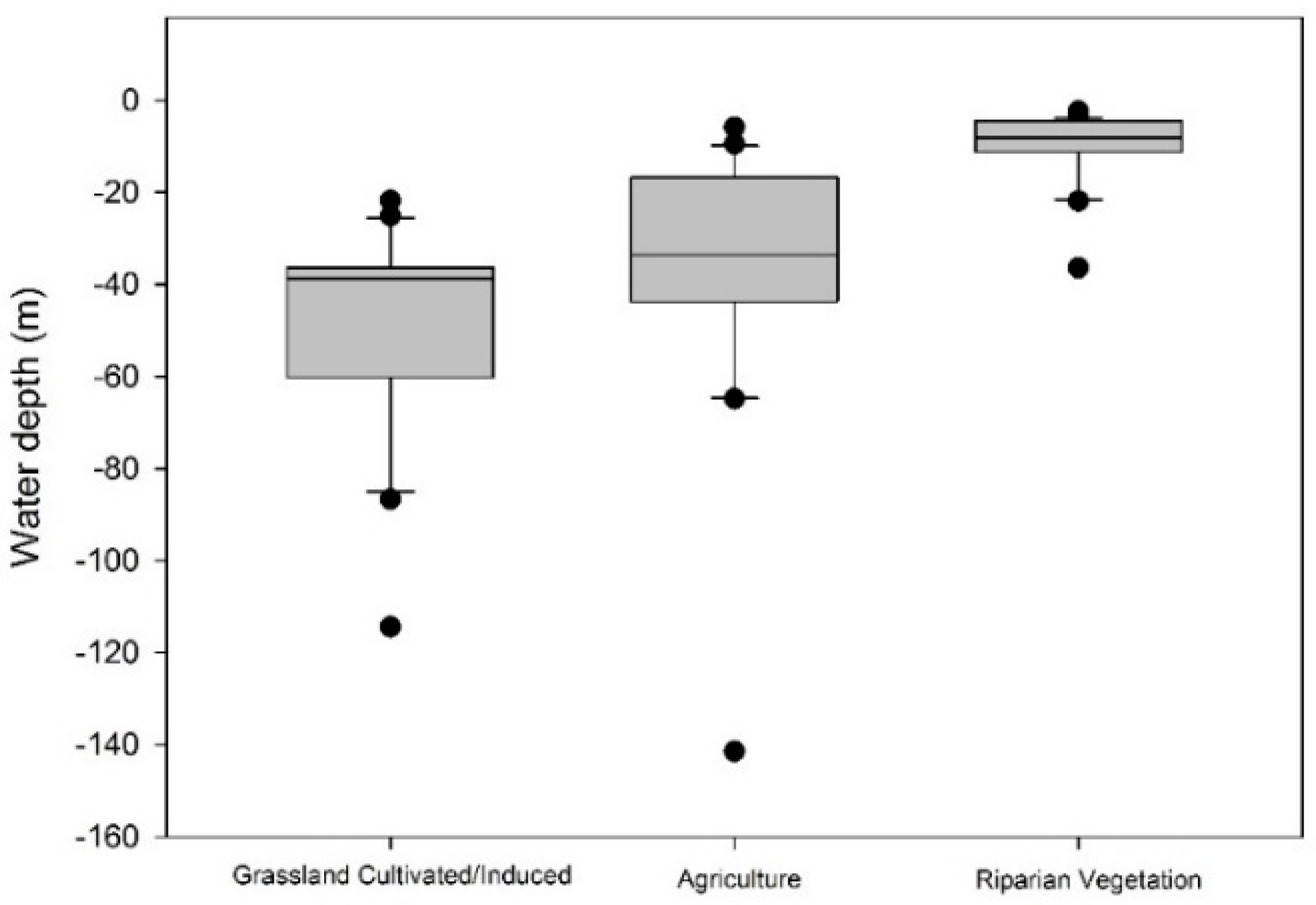
The results show a significant difference between Riparian Vegetation, Induced Grasslands and Agriculture in regard to water depth (ANOVA p < 0.01). Specifically, we found that Riparian Vegetation distributes in a much shallower water depth (mean = 9.9 m, CI 95% = 0–10.9 m) than grasslands (mean = 48.3 m CI 95% = 38.3–58.3 m) and Agriculture (mean = 37.1 m CI 95% = 26.9–47.4 m) (Figure 4).

The previous was expected since Riparian Vegetation is not characterized by very deep root systems even when the vegetation structure has been modified and some phreatophytes like Prosopis species are present. Even though the literature suggests that Riparian Vegetation will only be present at depths no greater than 7 m [71], it seems like some of the species present in these particular systems can reach deeper water sources. This confirms that grasslands are dependent on rainfall and upper soil humidity to trigger and maintain biological cycles [73]. Agriculture in this region is dependent on irrigation rather than ground water depth (or even rainfall) [23,25,26].

According to our results, we observed a greater depth of water on the ZR than the SMR. Our results suggest that deeper groundwater is related to agricultural development (Figure 5). We found that 70% of agricultural fields are associated with areas where groundwater depth is greater than 29 m. On the other hand, about 68% of the area covered by Riparian Vegetation in both sub-watersheds is associated with water depths of between 1 to 20 meters. Due to water extraction practices leading to the lowering of the ground water levels, agricultural areas that were previously RE have potentially crossed water depth thresholds necessary for the riparian vegetation to reestablish [71].

3.3.2. Changes in Riparian Vegetation (between 2002 and 2011) Related to Water Depth

Our results show that riparian cover converted mostly to Subtropical/Succulent Scrub in areas where the ground water levels were shallower than seven meters (

Table 9. Changes in riparian vegetation related to Water depth less than seven meters (changes from 2002 to 2011).

From	To	Ha
Riparian Vegetation	Agriculture	264
Riparian Vegetation	Bare Soil	106
Riparian Vegetation	Desert Scrub	108
Riparian Vegetation	Mesquite Woodland	122
Riparian Vegetation	Grassland Cultivated/Induced	27
Riparian Vegetation	Riparian Vegetation	3195
Riparian Vegetation	Subtropical/Succulent Scrub	2164
Riparian Vegetation	Natural Grassland	3
Agriculture	Riparian Vegetation	849
Bare Soil	Riparian Vegetation	4
Desert Scrub	Riparian Vegetation	82
Mesquite Woodland	Riparian Vegetation	178
Grassland Cultivated/Induced	Riparian Vegetation	5
Subtropical/Succulent Scrub	Riparian Vegetation	226
Forest (Oak and Oak/Pine)	Riparian Vegetation	<1
Natural Grassland	Riparian Vegetation	<1

). This was expected according to our ground water depth maps (Figure 4). The portions of the rivers that have the shallowest ground water occur mostly in the upper latitudes of the SMR where the adjacent vegetation is mostly Subtropical/Succulent Scrub.

The class that converted most to Riparian Vegetation, in areas where the ground water levels were deeper than seven meters, was Agriculture (

Table 10. Changes in Riparian Vegetation related to Water depth greater than seven meters (changes from 2002 to 2011).

From	To	Ha
Riparian Vegetation	Agriculture	781
Riparian Vegetation	Water	3
Riparian Vegetation	Bare Soil	58
Riparian Vegetation	Desert Scrub	699
Riparian Vegetation	Mesquite Woodland	2869
Riparian Vegetation	Grassland Cultivated/Induced	772
Riparian Vegetation	Riparian Vegetation	8181
Riparian Vegetation	Subtropical/Succulent Scrub	1980
Riparian Vegetation	Forest (Oak and Oak/Pine)	<1
Riparian Vegetation	Natural Grassland	2
Agriculture	Riparian Vegetation	1741
Water	Riparian Vegetation	6
Bare Soil	Riparian Vegetation	84
Desert Scrub	Riparian Vegetation	566
Mesquite Woodland	Riparian Vegetation	3728
Grassland Cultivated/Induced	Riparian Vegetation	1152
Subtropical/Succulent Scrub	Riparian Vegetation	1078
Forest (Oak and Oak/Pine)	Riparian Vegetation	45
Natural Grassland	Riparian Vegetation	1

). This can be explained by the fact that agricultural fields are highly managed systems, independent of ground water depth. The conversion of Riparian Vegetation to Mesquite Woodlands was apparent during field work and has been reported in the literature [17]. The change from Riparian Vegetation to phreatophytes with long and deep root systems, like Prosopis spp., might be a consequence of an increase in the depth of ground water [17,74].

Mesquite Woodland and Agriculture are the classes that converted most to Riparian Vegetation, a trend that seems to be unrelated to ground water depth. However, it seems that Riparian Vegetation might be able to persist in environments with ground water depths greater than 7 m when modified by vegetation from adjacent land cover types. Our results show a constant exchange between Mesquite Woodland and Riparian Vegetation this was expected since our field observations and the literature [17,29,75,76] indicate that mesquite dominated vegetation tend to replace or modify the structure of ecosystems including riparian habitats.

The net change in Riparian Vegetation using the 7 m threshold shows that riparian areas have not undergone significant reduction or increase. However, we believe that the functionality of the environment has been heavily modified. Based on a literature review [17,71,74,77,78] and field observations of exchange between Riparian Vegetation and Mesquite Woodlands we can say that mesquites are becoming common vegetation present on the rivers of this region.

4. Conclusions

This study addresses techniques and methodologies to use remote sensing products and derive tools for real applications regarding the study of riparian land cover in arid environments. Moreover, it highlights the usefulness of a classification and land cover change detection approach to obtain timely information for decision making in developing countries.

Specifically, in this study, we found evidence suggesting that threats to riparian habitats in arid environments might come from multiple human factors due to economic activities developed in specific areas. We were able to observe fluctuation in the riparian land cover with the introduction and implementation of nonnative grasses. We observed interchange between Mesquite Woodland, Subtropical/Succulent Scrub and Riparian Vegetation. We believe that further details of these interchanges might be exposed through the study of the relationship of vegetation types to factors such as ground water depth and climatic adaptation.

We were able to capture differences in distribution and change of land cover classes in relation to water depth. Our results agree with the idea that Riparian Vegetation distributes mostly in areas of shallow water (water depth less than 10 m). However, we also found that Riparian Vegetation might thrive in areas with deeper water depth than previously reported. As expected, land cover distribution, as a function of water depth, was key for Riparian Vegetation, but not for other land cover classes analyzed (Grassland Cultivated/Induced and Agriculture).

The RE in arid environments can be considered extremely diverse in terms of the number of species, processes, functions and usage (by humans) when compared to adjacent vegetation or land cover types. It is important to study these environments in arid lands; even though the area occupied by them is small, their importance is enormous for the life in these zones. Through remote sensing and spatial analysis we have been able to further our understanding on how “arid wetlands” interact with the environment and how they change through time.

References

- Costanza, R.; d’Arge, R.; Limburg, K.; Grasso, M.; de Groot, R.; Faber, S.; O’Neill, R.; van den Belt, M.; Paruelo, J.; Raskin, R. The value of the world’s ecosystem services and natural capital. Nature 1997, 387, 253–260. [Google Scholar] [CrossRef]
- Wilson, M.A.; Carpenter, S.R. Economic Valuation of Freshwater Ecosystem Services in the United States: 1971–1997. Ecol. Appl. 1999, 9, 772–783. [Google Scholar]
- Granados-Sánchez, D.; Hernández-García, M.; López-Ríos, G. Ecología de las zonas ribereñas. Rev. Chapingo Ser 2006, 12, 55–69. (In Spanish) [Google Scholar]
- Makkeasorn, A.; Chang, N.-B.; Li, J. Seasonal change detection of riparian zones with remote sensing images and genetic programming in a semi-arid watershed. J. Environ. Manag. 2009, 90, 1069–1080. [Google Scholar] [CrossRef] [PubMed]
- Zaimes, G.; Nichols, M.; Green, D.; Crimmins, M. Understanding Arizona’s Riparian Areas. College of Agriculture and Life Sciences, University of Arizona, Tucson, AZ, 2007. Available online: http://extension.arizona.edu/sites/extension.arizona.edu/files/pubs/az1432.pdf (accessed on 4 August 2016).
- Myers, N. Threatened biotas: “Hot spots“ in tropical forests. Environmentalist 1988, 8, 187–208. [Google Scholar] [CrossRef] [PubMed]
- Myers, N. The biodiversity challenge: Expanded hot-spots analysis. Environmentalist 1990, 10, 243–256. [Google Scholar] [CrossRef] [PubMed]
- De Groot, R.S.; Alkemade, R.; Braat, L.; Hein, L.; Willemen, L. Challenges in integrating the concept of ecosystem services and values in landscape planning, management and decision making. Ecol. Complex. 2010, 7, 260–272. [Google Scholar] [CrossRef]
- Loomis, J.; Kent, P.; Strange, L.; Fausch, K.; Covich, A. Measuring the total economic value of restoring ecosystem services in an impaired river basin: Results from a contingent valuation survey. Ecol. Econ. 2000, 33, 103–117. [Google Scholar] [CrossRef]
- Assessment, M.E. Ecosystems and Human Well-Being; Island Press: Washington, DC, USA, 2005; Volume 5. [Google Scholar]
- Orúe, M.E.; Booman, G.C.; Laterra, P. Uso de la tierra, configuración del paisaje y el filtrado de sedimentos y nutrientes por humedales y vegetación ribereña. In Valoración de Servicios Ecosistémicos: Conceptos, Herramientas y Aplicaciones Para el Ordenamiento Territorial; INTA Ediciones: Buenos Aires, Argentina, 2011; pp. 237–254. (In Spanish) [Google Scholar]
- Sweeney, B.W.; Bott, T.L.; Jackson, J.K.; Kaplan, L.A.; Newbold, J.D.; Standley, L.J.; Hession, W.C.; Horwitz, R.J. Riparian deforestation, stream narrowing, and loss of stream ecosystem services. Proc. Natl. Acad. Sci. USA 2004, 101, 14132–14137. [Google Scholar] [CrossRef] [PubMed]
- Ffolliott, P.F.; DeBano, L.F.; Baker, M.B., Jr.; Neary, D.G.; Brooks, K.N. Hydrology and impacts of disturbances on hydrologic function. In Riparian Areas of the Southwestern United States: Hydrology, Ecology, and Management; Baker, M.B., Ffolliott, P.F., DeBano, L.F., Neary, D.G., Eds.; CRC: Boca Raton, FL, USA, 2004; p. 51. [Google Scholar]
- Scott, M.L.; Nagler, P.L.; Glenn, E.P.; Valdes-Casillas, C.; Erker, J.A.; Reynolds, E.W.; Shafroth, P.B.; Gomez-Limon, E.; Jones, C.L. Assessing the extent and diversity of riparian ecosystems in Sonora, Mexico. Biodivers. Conserv. 2009, 18, 247–269. [Google Scholar] [CrossRef]
- Villarreal, M.L.; Van Leeuwen, W.J.; Romo-Leon, J.R. Mapping and monitoring riparian vegetation distribution, structure and composition with regression tree models and post-classification change metrics. Int. J. Remote Sens. 2012, 33, 4266–4290. [Google Scholar] [CrossRef]
- DeBano, L.F.; DeBano, S.J.; Wooster, D.E.; Baker, M.B., Jr. Linkages between riparian corridors and surrounding watersheds. In Riparian Areas of the Southwestern United States: Hydrology, Ecology, and Management; CRC Press LLC: Boca Raton, FL, USA, 2004; p. 408. [Google Scholar]
- Patten, D.T. Riparian ecosytems of semi-arid north america: Diversity and human impacts. Wetlands 1998, 18, 498–512. [Google Scholar] [CrossRef]
- Strauch, A.; Kapust, A.; Jost, C. Impact of livestock management on water quality and streambank structure in a semi-arid, African ecosystem. J. Arid Environ. 2009, 73, 795–803. [Google Scholar] [CrossRef]
- Arriaga, L.; Castellanos, A.E.; Moreno, E.; Alarcón, J. Potential ecological distribution of alien invasive species and risk assessment: A case study of buffel grass in arid regions of Mexico. Conserv. Biol. 2004, 18, 1504–1514. [Google Scholar] [CrossRef]
- Burquez-Montijo, A.; Miller, M.; Martinez-Yrizar, A.; Tellman, B. Mexican grasslands, thornscrub, and the transformation of the sonoran desert by invasive exotic buffelgrass (Pennisetum ciliare). In Invasive Exotic Species in the Sonoran Region; University of Arizona Press: Tuczon, AZ, USA, 2002; p. 424. [Google Scholar]
- Castellanos, A.; Yanes, F.; Valdez-Zamudio, D. Drought-Tolerant Exotic Buffelgrass and Desertification. In Weeds Across Borders: Proceedings of a North American Conference; University of Arizona Press: Tucson, Arizona, USA, 2002; pp. 99–112. [Google Scholar]
- Franklin, K.A.; Lyons, K.; Nagler, P.L.; Lampkin, D.; Glenn, E.P.; Molina-Freaner, F.; Markow, T.; Huete, A.R. Buffelgrass (Pennisetum ciliare) land conversion and productivity in the plains of Sonora, Mexico. Biol. Conserv. 2006, 127, 62–71. [Google Scholar] [CrossRef]
- Moreno-Vazquez, J.L. y Navarro-Navarro L.A. El fortalecimiento de la resilencia de corredores riparios áridos: Ecohidrología y toma de decisiones en la cuenca del río san miguel. Unpublished work. 2016. (In Spanish) [Google Scholar]
- Ffolliott, P.F.; DeBano, L.F. Riparian Areas of the Southwestern United States: Hydrology, Ecology, and Management; CRC Press: Boca Raton, FL, USA, 2003. [Google Scholar]
- Comisión Nacional del Agua (CONAGUA). Actualización de la disponibilidad media anual de agua subterránea acuífero (2625) Rio San Miguel estado de Sonora. Diario Oficial de la Federación 2009(a). Available online: http://www.conagua.gob.mx/OCNO07/Noticias/2625%20R%C3%ADo%20San%20Miguel.pdf (accessed on 4 August 2016).
- Comisión Nacional del Agua (CONAGUA). Actualización de la disponibilidad media anual de agua subterránea acuífero (2625) Rio Zanjon estado de Sonora. Diario Oficial de la Federación 2009(b). Available online: http://www.conagua.gob.mx/OCNO07/Noticias/2626%20R%C3%ADo%20Zanj%C3%B3n.pdf (accessed on 4 August 2016).
- Ames, C.R. Importance, Preservation, and Management of Riparian Habitat: A Symposium; Technical Report RM-43; USDA Forest Service Gen.: Denver, CO, USA, 1977; pp. 49–51. [Google Scholar]
- Belsky, A.J.; Matzke, A.; Uselman, S. Survey of livestock influences on stream and riparian ecosystems in the western United States. J. Soil Water Conserv. 1999, 54, 419–431. [Google Scholar]
- Nie, W.; Yuan, Y.; Kepner, W.; Nash, M.S.; Jackson, M.; Erickson, C. Assessing impacts of landuse and landcover changes on hydrology for the upper San Pedro watershed. J. Hydrol. 2011, 407, 105–114. [Google Scholar] [CrossRef]
- Webb, R.H.; Leake, S.A.; Turner, R.M. The Ribbon of Green: Change in Riparian Vegetation in the Southwestern United States; University of Arizona Press: Tucson, AZ, USA, 2007. [Google Scholar]
- Kepner, W.G.; Watts, C.J.; Edmonds, C.M.; Maingi, J.K.; Marsh, S.E.; Luna, G. A landscape approach for detecting and evaluating change in a semi-arid environment. J. Environ. Monit. Assess. 2000, 64, 179–195. [Google Scholar] [CrossRef]
- Mather, P.; Tso, B. Classification Methods for Remotely Sensed Data; CRC Press: Boca Raton, FL, USA, 2009. [Google Scholar]
- Jensen, J.R. Introductory Digital Image Processing: A Remote Sensing Perspective; University of South Carolina: Columbus, OH, USA, 1986. [Google Scholar]
- Lu, D.; Mausel, P.; Brondizio, E.; Moran, E. Change detection techniques. Int. J. Remote Sens. 2004, 25, 2365–2401. [Google Scholar] [CrossRef]
- Singh, A. Review article digital change detection techniques using remotely-sensed data. Int. J. Remote Sens. 1989, 10, 989–1003. [Google Scholar] [CrossRef]
- Longley, P. Geographic Information Systems and Science; John Wiley & Sons: Chichester, UK, 2005; p. 517. [Google Scholar]
- Bravo Peña, L.C.; Castellanos Villegas, A.E.; Doode Matsumoto, O.S. Sequía agropecuaria y vulnerabilidad en el centro oriente de sonora: Un caso de estudio enfocado a la actividad ganadera de producción y exportación de becerros. Estudios Soc. (Hermosillo Son.) 2010, 18, 209–241. (In Spanish) [Google Scholar]
- INEGI. Red hidrográfica escala 1:50,000 edición 2.0. Available online: http://www.Inegi.Org.Mx/geo/contenidos/topografia/descarga.Aspx (accesed on 11 June 2016).
- CONAGUA. Programa de Medidas Preventivas y de Mitigación de la Sequía para el Consejo de Cuenca alto Noroeste. Programa Nacional Contra la Sequía (PRONACOSE). Available online: http://www.Pronacose.Gob.Mx/Pronacose14/Contenido/Documentos/Imta_Conagua%20cuenca%20noroeste%20salida.Pdf (accessed on 18 November 2015).
- Universidad de Sonora (UNISON). Estudio geohidrológico de las subcuencas de los ríos Sonora, Zanjon, San Miguel, Mesa del Seri-La Victoria y cuenca Bacoachito. Informe final. Comisión Estatal del Agua. Unpublished Work. 2005. (In Spanish) [Google Scholar]
- Shreve, F.; Wiggins, I.L. Vegetation and Flora of the Sonoran Desert. Vols. 1 and 2; Stanford University Press: Stanford, CA, USA, 1964; pp. 1–840. [Google Scholar]
- Secretaría de Agricultura y Recursos Hidráulicos (SARH). Inventario Forestal Nacional periódico, México 94, Memoria Nacional. Secretaria de Agricultura y Recursos Hidráulicos, Subsecretaría Forestal y de Fauna Silvestre, México, D.F. 1994. Available online: http://repositorio.inecc.gob.mx/ae2/ae_333.750972_m495-08i_1994.pdf (accesed on 2 February 2016). (In Spanish)
- Nabhan, G.P.; Sheridan, T.E. Living fencerows of the Rio San Miguel, Sonora, Mexico: Traditional technology for floodplain management. Hum. Ecol. 1977, 5, 97–111. [Google Scholar] [CrossRef]
- Romo-Leon, J.R.; van Leeuwen, W.J.; Castellanos-Villegas, A. Using remote sensing tools to assess land use transitions in unsustainable arid agro-ecosystems. J. Arid Environ. 2014, 106, 27–35. [Google Scholar] [CrossRef]
- USGS. Earthexplorer. Available online: http://earthexplorer.usgs.gov/ (accessed on 18 July 2014).
- Ju, J.; Roy, D.P.; Vermote, E.; Masek, J.; Kovalskyy, V. Continental-scale validation of MODIS-based and LEDAPS landsat ETM+ atmospheric correction methods. Remote Sens. Environ. 2012, 122, 175–184. [Google Scholar] [CrossRef]
- Wolfe, R.; Masek, J.; Saleous, N.; Hall, F. Ledaps: Mapping North American Disturbance from the Landsat Record. In Proceedings of the 2004 IEEE International Geoscience and Remote Sensing Symposium (IGARSS’04), Anchorage, AK, USA, 20–24 September 2004.
- Anderson, J.R. A Land Use and Land Cover Classification System for Use with Remote Sensor Data; US Government Printing Office: Washington, DC, USA, 1976; Volume 964.
- Coppin, P.; Jonckheere, I.; Nackaerts, K.; Muys, B.; Lambin, E. Review articledigital change detection methods in ecosystem monitoring: A review. Int. J. Remote Sens. 2004, 25, 1565–1596. [Google Scholar] [CrossRef]
- Shalaby, A.; Tateishi, R. Remote sensing and GIS for mapping and monitoring land cover and land-use changes in the Northwestern coastal zone of Egypt. Appl. Geogr. 2007, 27, 28–41. [Google Scholar] [CrossRef]
- Breiman, L.; Friedman, J.; Olshen, R.; Stone, C.J.; Olshen, R.A. Classification and Regression Trees; CRC Press: Belmont, CA, USA, 1984. [Google Scholar]
- Roe, B.P.; Yang, H.J.; Zhu, J.; Liu, Y.; Stancu, I.; McGregor, G. Boosted Decision Trees as an Alternative to Artificial Neural Networks for Particle Identification. Nucl. Instrum. Meth. A 2005, 543, 577–584. [Google Scholar] [CrossRef]
- De’ath, G.; Fabricius, K.E. Classification and regression trees: A powerful yet simple technique for ecological data analysis. Ecology 2000, 81, 3178–3192. [Google Scholar] [CrossRef]
- De Fries, R.; Hansen, M.; Townshend, J.; Sohlberg, R. Global land cover classifications at 8 km spatial resolution: The use of training data derived from Landsat imagery in decision tree classifiers. Int. J. Remote Sens. 1998, 19, 3141–3168. [Google Scholar] [CrossRef]
- Friedl, M.A.; McIver, D.K.; Hodges, J.C.; Zhang, X.; Muchoney, D.; Strahler, A.H.; Woodcock, C.E.; Gopal, S.; Schneider, A.; Cooper, A. Global land cover mapping from MODIS: Algorithms and early results. Remote Sens. Environ. 2002, 83, 287–302. [Google Scholar] [CrossRef]
- Tucker, C.J. Red and photographic infrared linear combinations for monitoring vegetation. Remote Sens. Environ. 1979, 8, 127–150. [Google Scholar] [CrossRef]
- Avery, T.E.; Berlin, G.L. Fundamentals of Remote Sensing and Airphoto Interpretation; Macmillan: New York, NY, USA, 1992. [Google Scholar]
- Huete, A.R. A soil-adjusted vegetation index (SAVI). Remote Sens. Environ. 1988, 25, 295–309. [Google Scholar] [CrossRef]
- Van Leeuwen, W.J.; Huete, A.R.; Laing, T.W. MODIS vegetation index compositing approach: A prototype with AVHRR data. Remote Sens. Environ. 1999, 69, 264–280. [Google Scholar] [CrossRef]
- Huete, A.; Didan, K.; Miura, T.; Rodriguez, E.P.; Gao, X.; Ferreira, L.G. Overview of the radiometric and biophysical performance of the MODIS vegetation indices. Remote Sens. Environ. 2002, 83, 195–213. [Google Scholar] [CrossRef]
- Crist, E.P.; Cicone, R.C. A physically-based transformation of Thematic Mapper data—The TM tasseled cap. IEEE Trans. Geosci. Remote Sens. 1984, 22, 256–263. [Google Scholar] [CrossRef]
- Collins, J.B.; Woodcock, C.E. An assessment of several linear change detection techniques for mapping forest mortality using multitemporal Landsat TM data. Remote Sens. Environ. 1996, 56, 66–77. [Google Scholar] [CrossRef]
- Asner, G.P.; Keller, M.; Pereira, R.; Zweede, J.C. Remote sensing of selective logging in amazonia: Assessing limitations based on detailed field observations, Landsat ETM+, and textural analysis. Remote Sens. Environ. 2002, 80, 483–496. [Google Scholar] [CrossRef]
- Congalton, R.G. A review of assessing the accuracy of classifications of remotely sensed data. Remote Sens. Environ. 1991, 37, 35–46. [Google Scholar] [CrossRef]
- Foody, G.M. Status of land cover classification accuracy assessment. Remote Sens. Environ. 2002, 80, 185–201. [Google Scholar] [CrossRef]
- Rogan, J.; Franklin, J.; Roberts, D.A. A comparison of methods for monitoring multitemporal vegetation change using Thematic Mapper imagery. Remote Sens. Environ. 2002, 80, 143–156. [Google Scholar] [CrossRef]
- Congalton, R.G.; Green, K. Assessing the Accuracy of Remotely Sensed Data: Principles and Practices; CRC Press: Boca Raton, FL, USA, 2008. [Google Scholar]
- Díaz-Caravantes, R.E.; Sánchez-Flores, E. Water transfer effects on peri-urban land use/land cover: A case study in a semi-arid region of Mexico. Appl. Geogr. 2011, 31, 413–425. [Google Scholar] [CrossRef]
- Nguyen, U.; Glenn, E.P.; Nagler, P.L.; Scott, R.L. Long-term decrease in satellite vegetation indices in response to environmental variables in an iconic desert riparian ecosystem: The upper San Pedro, Arizona, United States. Ecohydrology 2015, 8, 610–625. [Google Scholar] [CrossRef]
- Bravo Peña, L.C.; Doode Matsumoto, O.S.; Castellanos Villegas, A.E.; Espejel Carbajal, I. Políticas rurales y pérdida de cobertura vegetal: Elementos para reformular instrumentos de fomento agropecuario relacionados con la apertura de praderas ganaderas en el noroeste de méxico. Reg. Soc. 2010, 22, 3–35. (In Spanish) [Google Scholar]
- Stromberg, J.; Tiller, R.; Richter, B. Effects of groundwater decline on riparian vegetation of semiarid regions: The San Pedro, Arizona. Ecol. Appl. 1996, 6, 113–131. [Google Scholar] [CrossRef]
- Gunderson, L.H. Ecological resilience—In theory and application. Annu. Rev. Ecol. Syst. 2003, 31, 425–439. [Google Scholar] [CrossRef]
- Michel, H.C.; Oliva, F.G.; Rodríguez, J.C.; Villegas, A.E.C. Cambios en el almacenamiento de nitrógeno y agua en el suelo de un matorral desértico transformado a sabana de buffel (Pennisetum ciliare (L.) link). Rev. Terra Latinoam. 2015, 33, 79–94. (In Spanish) [Google Scholar]
- Stromberg, J.C.; McCluney, K.; Dixon, M.; Meixner, T. Dryland riparian ecosystems in the American southwest: Sensitivity and resilience to climatic extremes. Ecosystems 2013, 16, 1–5. [Google Scholar] [CrossRef]
- Pierini, N.A.; Vivoni, E.R.; Robles-Morua, A.; Scott, R.L.; Nearing, M.A. Using observations and a distributed hydrologic model to explore runoff thresholds linked with mesquite encroachment in the Sonoran Desert. Water Resour. Res. 2014, 50, 8191–8215. [Google Scholar] [CrossRef]
- Scott, R.L.; Huxman, T.E.; Williams, D.G.; Goodrich, D.C. Ecohydrological impacts of woody-plant encroachment: Seasonal patterns of water and carbon dioxide exchange within a semiarid riparian environment. Glob. Chang. Biol. 2006, 12, 311–324. [Google Scholar] [CrossRef]
- Stromberg, J.C.; Lite, S.J.; Rychener, T.J.; Levick, L.R.; Dixon, M.D.; Watts, J.M. Status of the riparian ecosystem in the upper San Pedro river, Arizona: Application of an assessment model. Environ. Monit. Assess. 2006, 115, 145–173. [Google Scholar] [CrossRef] [PubMed]
- House-Peters, L.A.; Scott, C.A. Assessing the impacts of land use change on water availability, management, and resilience in arid region riparian corridors: A case study of the San Pedro and Rio Sonora watersheds in southwestern USA and northwestern Mexico. In Procedings of the XIV World Water Congress of the International Water Resources Association, Porto de Galinhas, Brazil, 25–29 September 2011.
© 2016 by the authors; licensee MDPI, Basel, Switzerland. This article is an open access article distributed under the terms and conditions of the Creative Commons Attribution (CC-BY) license (http://creativecommons.org/licenses/by/4.0/).