
An Image Matching Algorithm Integrating Global SRTM and Image Segmentation for Multi-Source Satellite Imagery

Abstract
:
1. Introduction
- Since multi-source satellite images are acquired from different sensors and perspectives, there are large geometric distortions between them (e.g., resolution difference, rotation, projection disparity, etc.). These distortions may decrease the correlation between correspondences and even may make the current matching algorithms invalid.
- To achieve numerous correspondences, the geometry constraint of triangulations is employed by many matching algorithms [3,4,5]. The key to this kind of constraint is that each triangle is assumed to be a locally planar area. However, for areas with large topographic relief (e.g., urban areas and mountain areas), the assumption fails, which seriously affects the matching reliability.
1.1. Related Studies
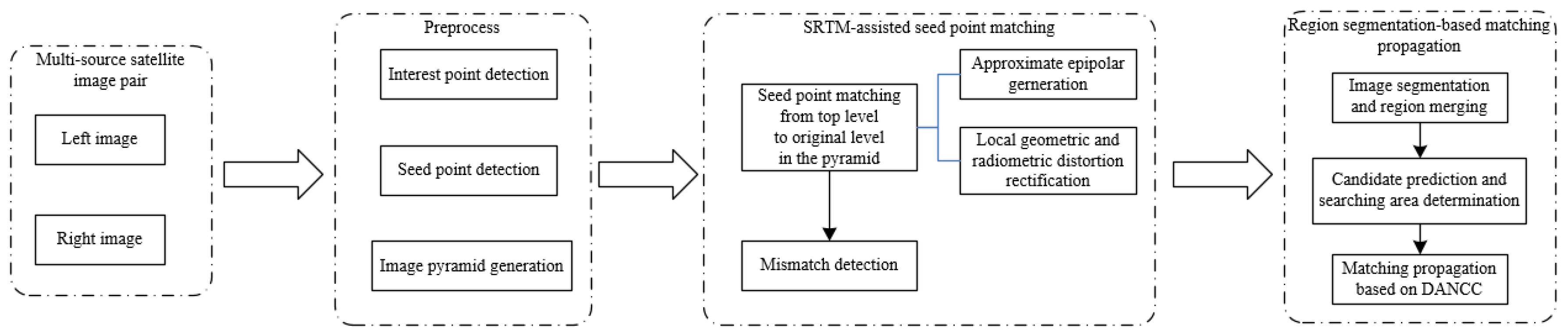
1.2. The Proposed Approach
- Based on the analysis of problems in the existing matching methods, considering the characteristics of multi-source satellite imagery, this paper develops a seed point matching method assisted by global SRTM. By the following research, the seed point selection, epipolar line generation, matching strategy optimization and mismatch detection, we can access reliable and high-precision corresponding points. Then, the corresponding points act as the seeds, which can provide reliable prior knowledge for the subsequent matching propagation.
- In order to obtain dense matching results, we propose a matching propagation method based on region segmentation. In this method, image segmentation technology is adopted innovatively in image matching algorithm in photogrammetry. Using the segmented regions as regional constraints, combined with the radiometric and geometric similarity, we constructed Distance, Angle and Normalized Cross-Correlation (DANCC), aiming at enhancing the validity of the texture-poor regions and repeat regions and to improve the accuracy rate and robustness of matching propagation.
2. Global SRTM-Assisted Seed Point Matching
2.1. Seed Point Selection
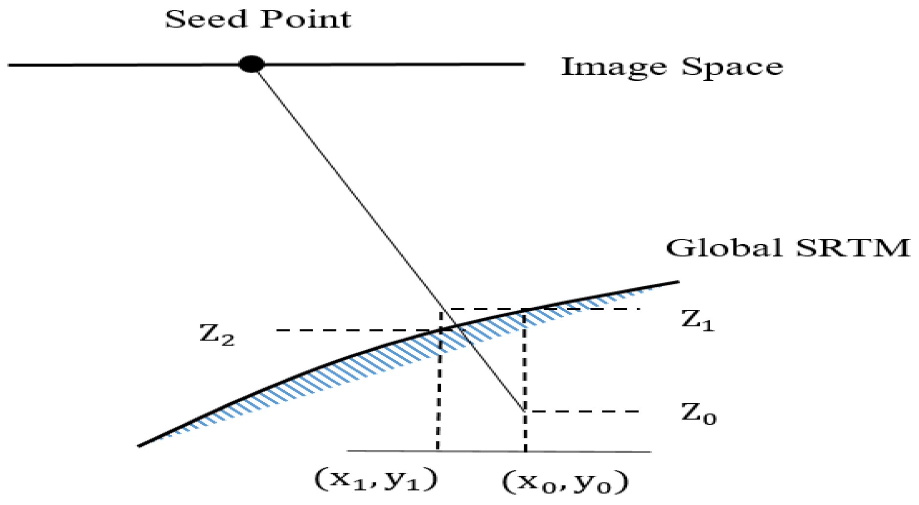
2.2. Epipolar Line Generation
2.3. Local Geometric and Radiometric Distortion Rectification
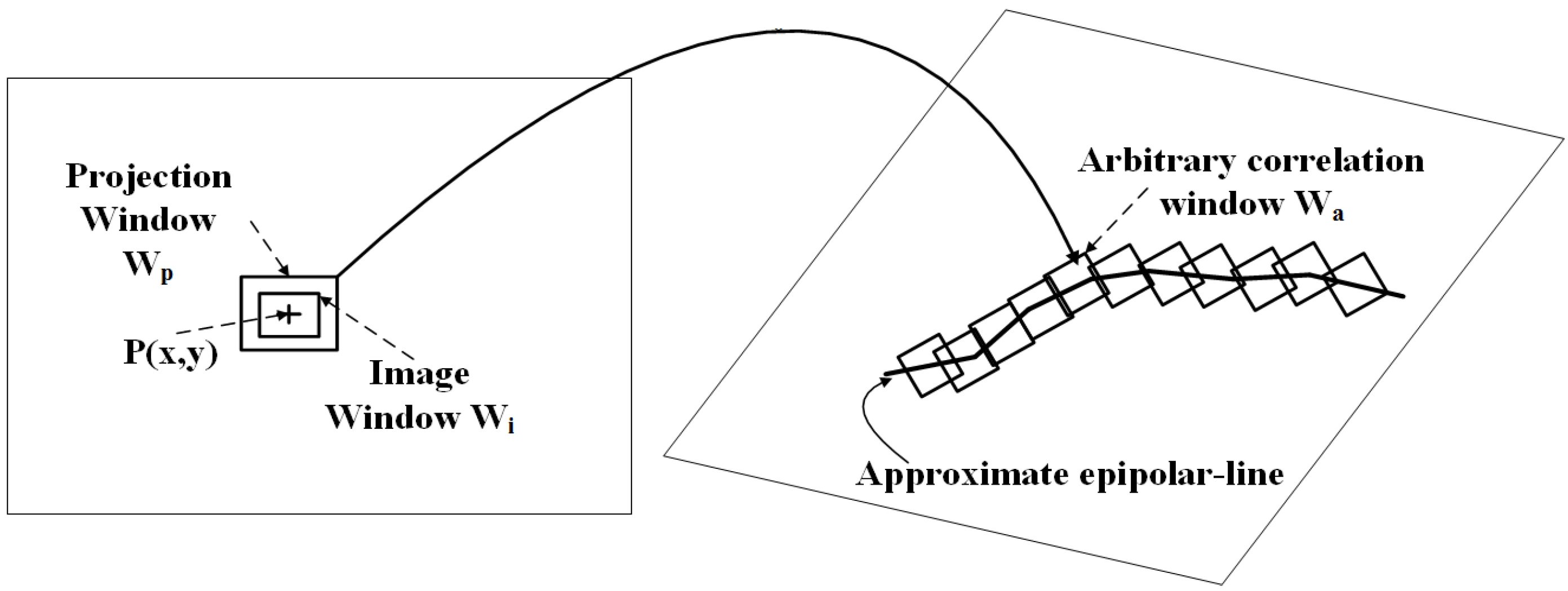
- For a height , which has been mentioned in Section 2.2, forward-project and backward-project (Equation (1)) the projection window , which includes this search area in the right image.where denotes the RFM of the left image, denotes the RFM of the right image and here are image coordinates of an arbitrary node of projection window .
- Use Equation (2) to calculate the affine transformation and linear radiometric transformation parameters between projection window and the correlation window .where and are obtained from the step above, are variables of affine transformation, and represent the left and right image gray value, respectively, and are the variables of linear radiometric transformation.
- Apply the transformation parameters to resample the correlation window to the projection window.
- For each pixel P in the projection window, compute the correlation coefficient between P and the seed point . Record the local maximum correlation coefficient and use affine transformation parameters to transform its coordinates back to the right image.
- Repeat all steps above over ; find the maximum correlation coefficient, and report it as the correspondence of the seed point.
2.4. Matching Strategy
3. Region Segmentation-Based Matching Propagation
3.1. Image Segmentation
3.2. Candidate Prediction
- Apply Equation (1) to compute forecast coordinates of seed point on the right image with height value Z mentioned in Section 2.2.
- Compute translation parameters from:where are the right image coordinates of the correspondence of seed point .
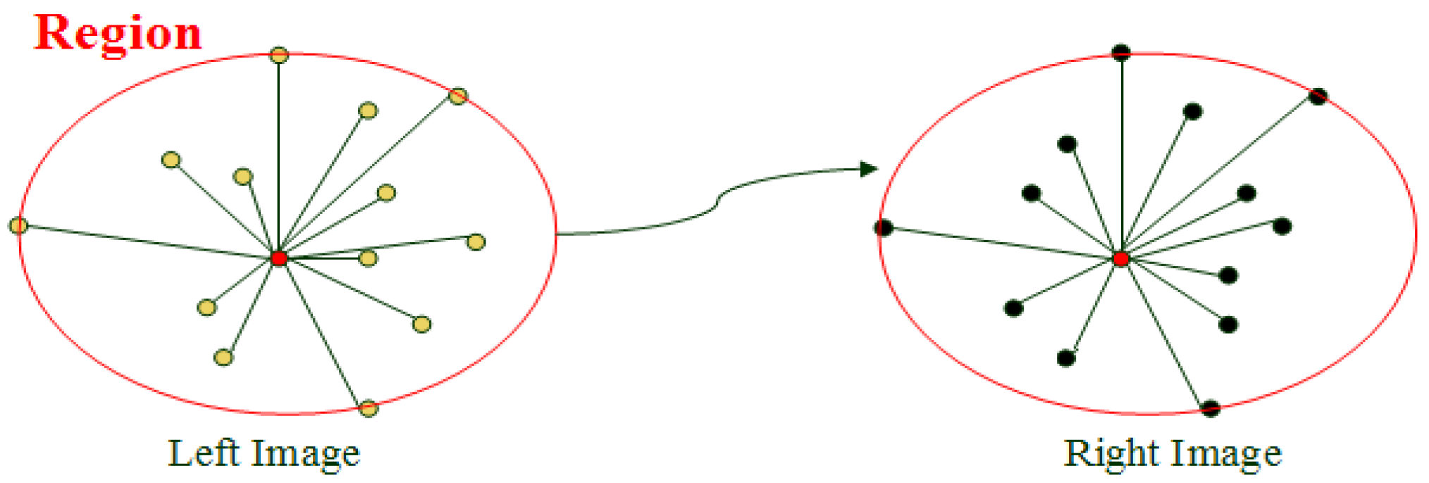
- All interest points within the same segment will be predicted on the right image from:If is in the same segment with the correspondence of the seed point, it will become the remaining point, as seen in Figure 9.
3.3. Searching Area Determination
3.4. Constraints for Matching Propagation
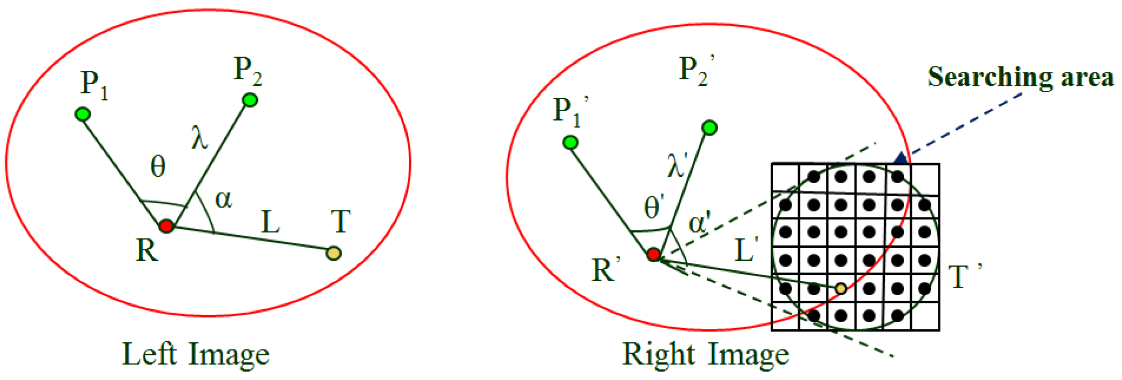
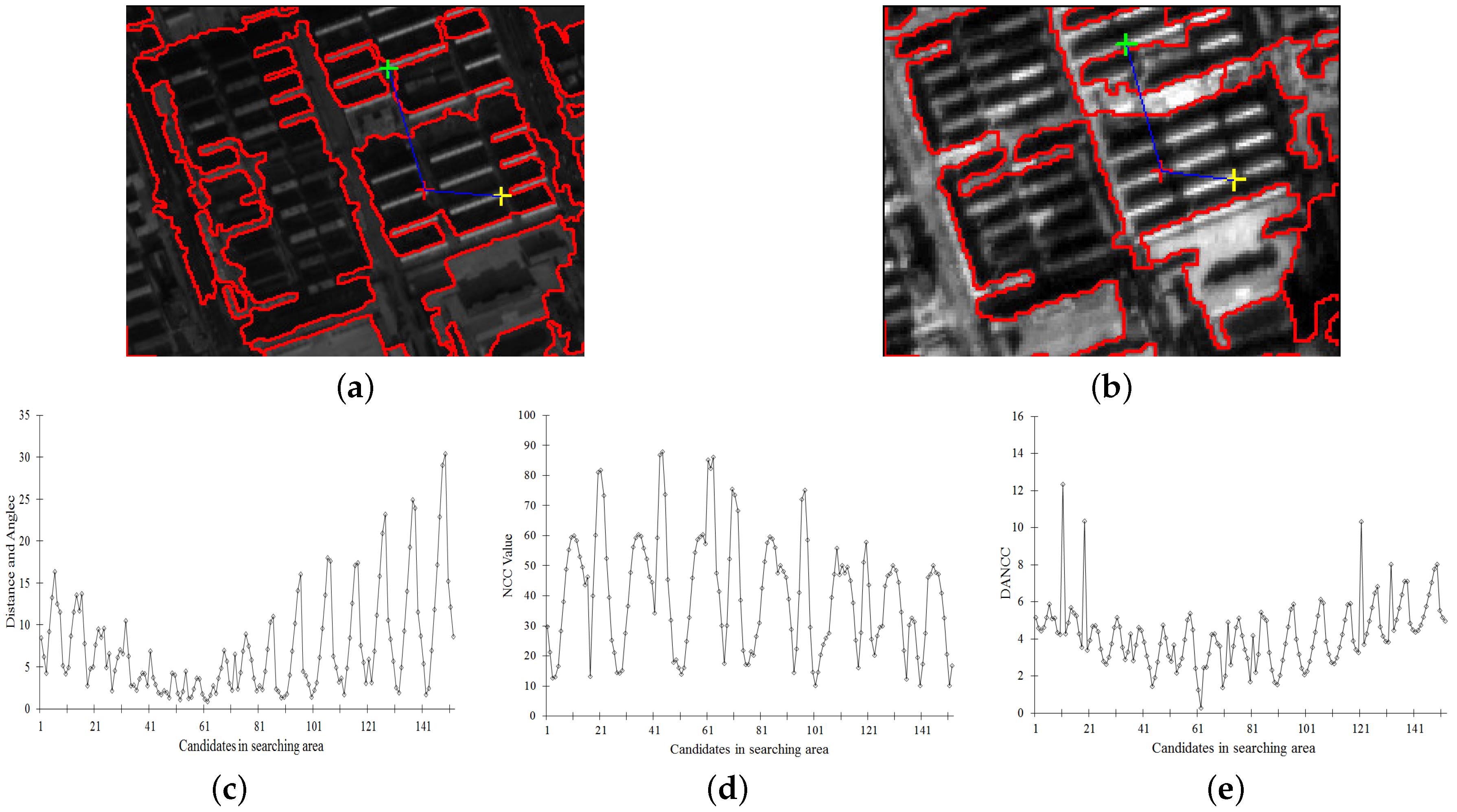
- Segmentation constraint: As seen in Figure 10, the corresponding seed points R and lie within their respective regions in the left and right images, so both regions are assumed to be the corresponding regions (i.e., the correspondence of the remaining point T in left image should be first identified within the corresponding region in the right image). This constraint is helpful for pixels inside the corresponding region in order to raise the priority for being the correspondence.
- Spatial distance constraint: In a locally planar area, the spatial distance between the remaining points and the root node should be relatively consistent. Therefore, a weighted constraint based on spatial distance is employed. As seen in Figure 10, the closer the distance between root node and a candidate in a searching area is to a threshold, the higher weight the candidate is assigned. The threshold is defined by , where is estimated as in Section 3.3.
- Spatial angle constraint: As seen in Figure 10, when point in the right image is assumed to be the correspondence of remaining point T in the left image, the intersection angle α should be consistent with angle in a locally planar area. Therefore, a weighted constraint based on spatial orientation is employed. When the intersection angle between a candidate and the two seed points in the right image is closer to a certain threshold, this candidate is assigned a higher weight, and the probability of correspondence is higher. The threshold is defined by , where is estimated as in Section 3.3.
3.5. An Integrated Similarity Measure (DANCC)
- Each region in the left image is considered to be an independently locally planar area, in which the seed point with the minimum error calculated by mismatch detection is selected as the root node. Another seed point nearest from the root node is selected as the starting node, after which the candidates for all remaining points that lie within the same region are predicted and the searching areas are determined.
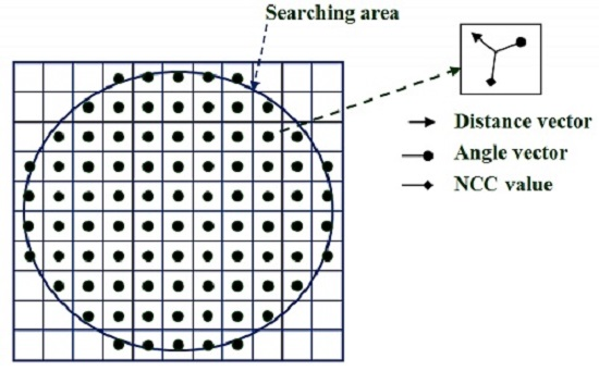
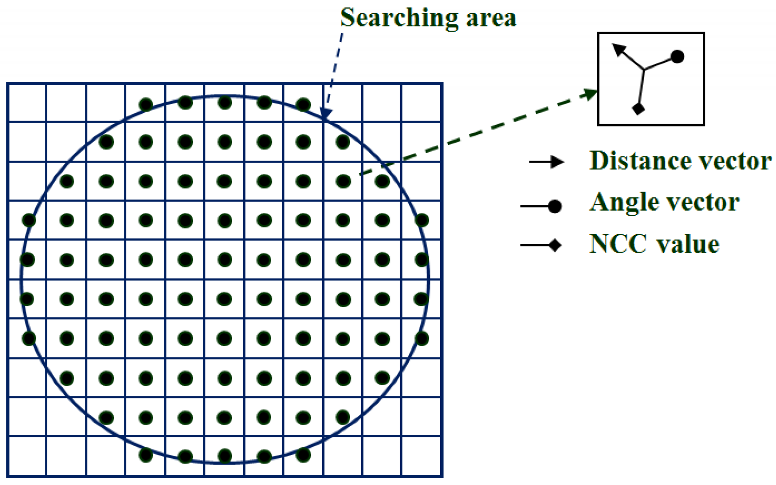
- NCC is employed to calculate the correlation values for all of the sample points in the searching areas. Moreover, distance and intersection angle are assigned to them. Three element vectors therefore are used to describe each sample point, as shown in Figure 11.
- 3.
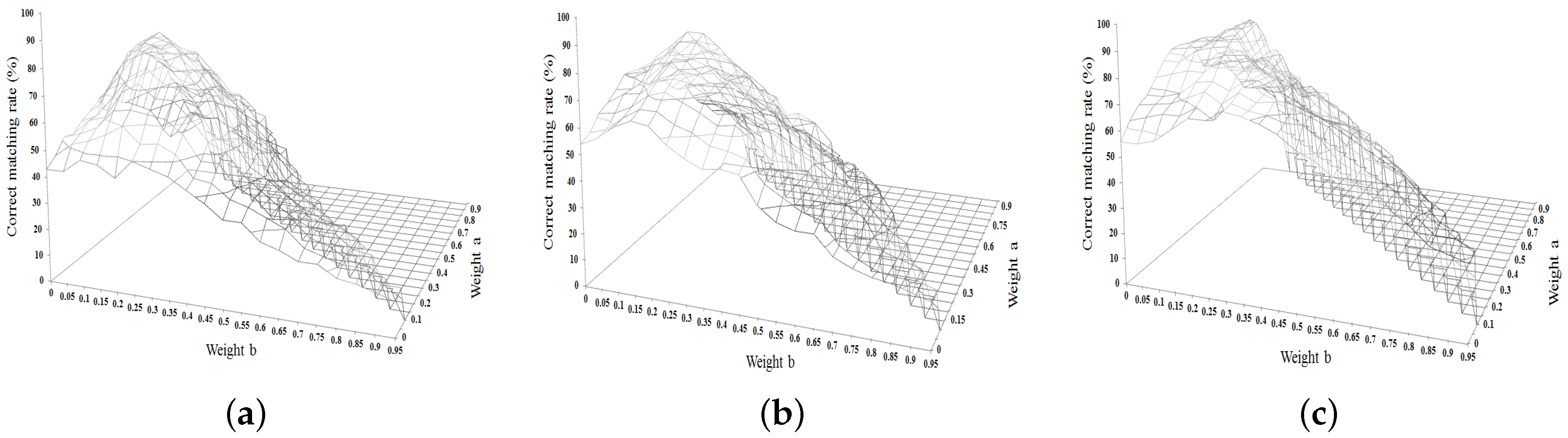
- The best candidate for each remaining point is found by identifying its nearest neighbor in the database of sample points. The nearest neighbor is defined with the minimum Euclidean distance, which is described in Equation (6). is the average correlation value in the searching area. and are both calculated as in Section 3.4. In addition, a, b are the weight values of the distance and angle vectors , which are estimated in the following section.
- 4.
- For each region containing seed points, the correspondences of the remaining points that belong to this region are obtained by DANCC. In addition, when a remaining point is matched in this region, the new correspondence becomes a candidate for the starting node. If the angle θ assigned to a remaining point is close to zero, the starting node is changed. After the remaining points within this region are matched, they are grouped to expand to the regions that do not contain seed points. These regions select the joint correspondences or closest correspondences as root nodes and starting nodes, and the matching propagation is performed in these regions using Step 1–Step 3.
3.6. Weight Value Estimation
4. Experimental Result and Analysis
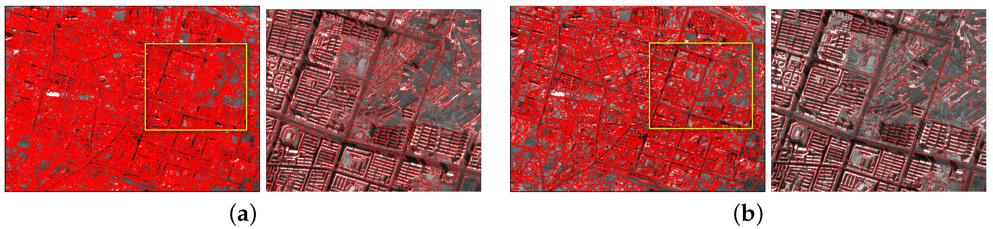
4.1. Experimental Results of Test 1
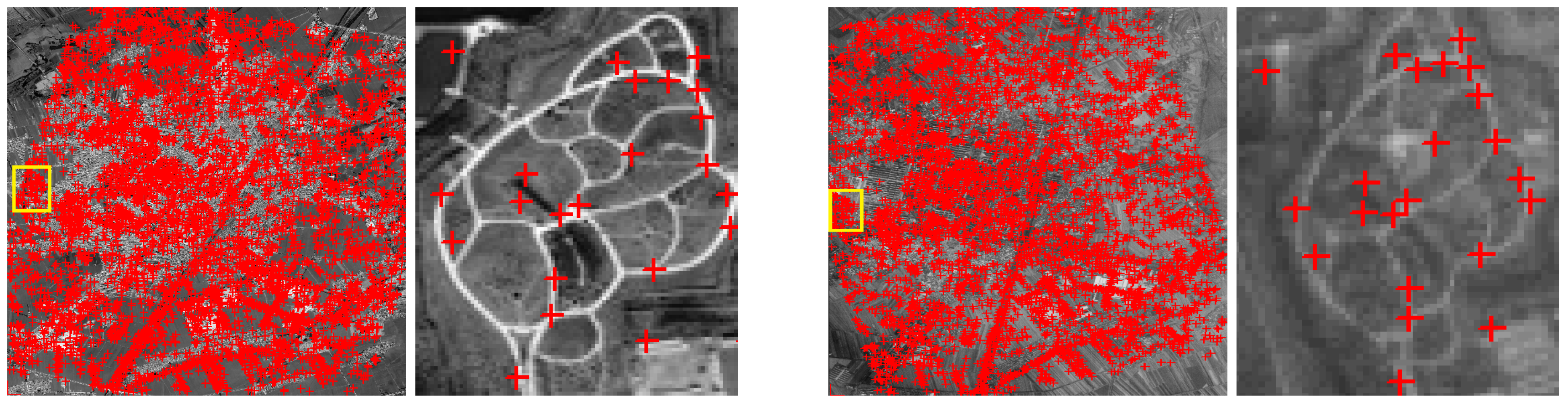
4.2. Experimental Results of Test 2
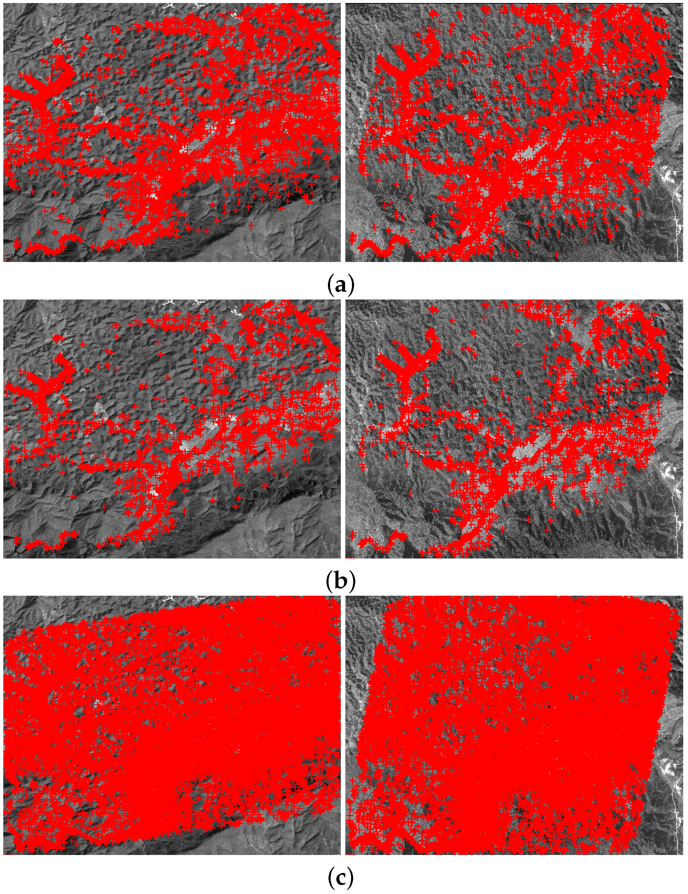
4.3. Experimental Results of Test 3
5. Conclusions
- This matching algorithm is fairly practical and effective for multi-source satellite images, which would be helpful in efforts to combine existing mass satellite data into a digital photogrammetry system.
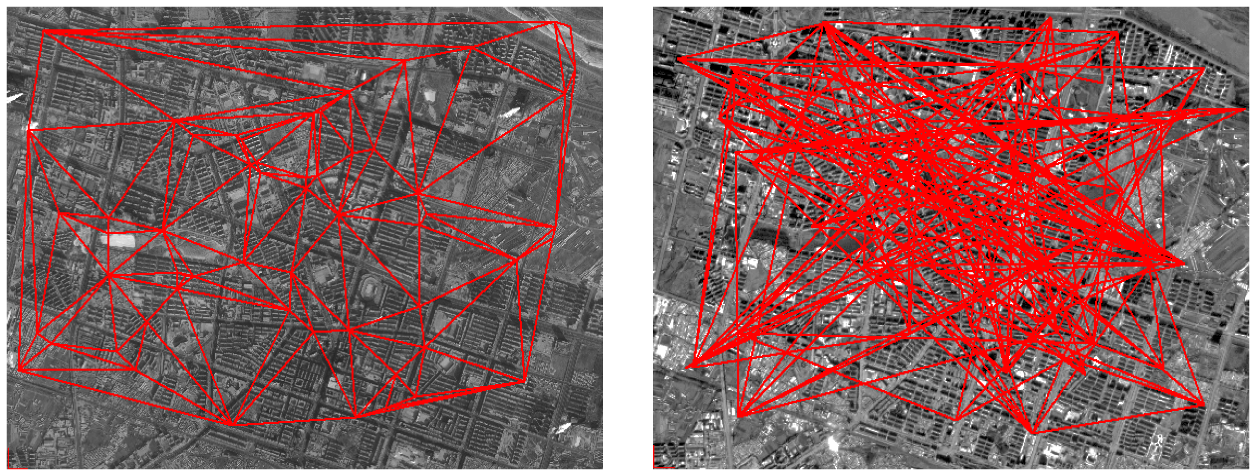
- For satellite images with large geometric distortions, this algorithm is capable of obtaining dense and reliable matching results. In addition, its region segmentation-based matching propagation performed quite well for image matching on repetitive or homogeneous textural images, for which achieving robust correspondences is difficult for existing methods.
Acknowledgments
Author Contributions
Conflicts of Interest
References
- Gruen, A. Development and status of image matching in photogrammetry. Photogramm. Rec. 2012, 27, 36–57. [Google Scholar] [CrossRef]
- Hartley, R.; Zisserman, A. Multiple View Geometry in Computer Vision, 2nd ed.; Cambridge University Press: Cambridge, UK, 2003; pp. 672–674. [Google Scholar]
- Wu, B.; Zhang, Y.S.; Zhu, Q. Integrated point and edge matching on poor textural images constrained by self-adaptive triangulations. ISPRS J. Photogramm. Remote Sens. 2012, 68, 40–55. [Google Scholar] [CrossRef]
- Wu, B.; Zhang, Y.S.; Zhu, Q. A Triangulation-based Hierarchical Image Matching Method for Wide-Baseline Images. Photogramm. Eng. Remote Sens. 2011, 77, 695–708. [Google Scholar] [CrossRef]
- Zhu, Q.; Wu, B.; Tian, Y.X. Propagation strategies for stereo image matching based on the dynamic triangle constraint. ISPRS J. Photogramm. Remote Sens. 2007, 62, 295–308. [Google Scholar] [CrossRef]
- Bleyer, M.; Gelautz, M. A layered stereo matching algorithm using image segmentation and global visibility constraints. ISPRS J. Photogramm. Remote Sens. 2005, 59, 128–150. [Google Scholar] [CrossRef]
- Heipke, C.; Oberst, J.; Albertz, J.; Attwenger, M.; Dorninger, P. Evaluating planetary digital terrain models-The HRSC DTM test. Planet. Space Sci. 2007, 55, 2173–2191. [Google Scholar] [CrossRef]
- Zhang, L. Automatic Digital Surface Model (DSM) Generation from Linear Array Images. Ph.D. Thesis, Swiss Federal Institute of Technology, Zurich, Switzerland, 2005. [Google Scholar]
- Google Satellite Images. Available online: http://www.google.com/earth/index.html (accessed on 14 April 2013).
- Helava, U. Digital correlation in photogrammetric instruments. Photogrammetria 1978, 34, 19–41. [Google Scholar] [CrossRef]
- Lhuillier, M.; Quan, L. Match propagation for image-based modeling and rendering. IEEE Trans. Pattern Anal. Mach. Intell. 2002, 24, 1140–1146. [Google Scholar] [CrossRef]
- Lowe, D.G. Distinctive Image Features from Scale-Invariant Keypoints. Int. J. Comput. Vis. 2004, 60, 91–110. [Google Scholar] [CrossRef]
- Ai, M.; Hu, Q.W.; Li, J.Y.; Wang, M.; Yuan, H. A Robust Photogrammetric Processing Method of Low-Altitude UAV Images. Remote Sens. 2015, 7, 2302–2333. [Google Scholar] [CrossRef]
- Mikolajczyk, K.; Schmid, C. Scale & Affine Invariant Interest Point Detectors. Int. J. Comput. Vis. 2004, 60, 63–86. [Google Scholar]
- Long, T.F.; Jiao, W.L.; He, G.J.; Zhang, Z.M. A Fast and Reliable Matching Method for Automated Georeferencing of Remotely-Sensed Imagery. Remote Sens. 2016, 8, 56. [Google Scholar] [CrossRef]
- Silveira, M.; Feitosa, R.; Jacobsen, K.; Brito, J.; Heckel, Y. A Hybrid Method for Stereo Image Matching. In Proceedings of the the International Archives of the Photogrammetry, Remote Sensing and Spatial Information Sciences, Beijing, China, 3–11 July 2008; pp. 895–901.
- Xiong, Z. Technical Development for Automatic Aerial Triangulation of High Resolution Satellite Imagery. Ph.D. Thesis, University of New Brunswick, Fredericton, NB, Canada, 2009. [Google Scholar]
- Xiong, Z.; Zhang, Y. A Novel Interest-Point-Matching Algorithm for High-Resolution Satellite Images. IEEE Trans. Geosci. Remote Sens. 2009, 47, 4189–4200. [Google Scholar] [CrossRef]
- IAlruzouq, R.; Habib, A. Semi-Automatic Registration of Multi-Source Satellite Imagery with Varying Geometric Resolutions. Photogramm. Eng. Remote Sens. 2005, 71, 325–332. [Google Scholar]
- Colerhodes, A.; Johnson, K.; PLemoigne, J.; Zavorin, I. Multiresolution registration of remote sensing imagery by optimization of mutual information using a stochastic gradient. IEEE Trans. Image Process. 2003, 12, 1495–1511. [Google Scholar] [CrossRef] [PubMed]
- Eugenio, F.; Marques, F. Automatic satellite image georeferencing using a contour-matching approach. IEEE Trans. Geosci. Remote Sens. 2003, 41, 2869–2880. [Google Scholar] [CrossRef]
- Chen, M.; Shao, Z.F. Robust affine-invariant line matching for high resolution remote sensing images. Photogramm. Eng. Remote Sens. 2013, 79, 753–760. [Google Scholar] [CrossRef]
- Hirschmüller, H. Accurate and efficient stereo processing by semi-global matching and mutual information. In Proceedings of the 2005 IEEE Computer Society Conference on Computer Vision and Pattern Recognition, San Diego, CA, USA, 20–25 June 2005; Volume 2, pp. 807–814.
- Hirschmüller, H. Stereo Processing by Semiglobal Matching and Mutual Information. IEEE Trans. Pattern Anal. Mach. Intell. 2008, 30, 328–341. [Google Scholar] [CrossRef] [PubMed]
- Hirschmüller, H. Semi-global matching-motivation, developments and applications. In Proceedings of the Photogrammetric Week 11, Stuttgart, Germany, 5–9 September 2011.
- Humenberger, M.; Engelke, T.; Kubinger, W. A census-based stereo vision algorithm using modified semi-global matching and plane fitting to improve matching quality. In Proceedings of the 2010 IEEE Computer Society Conference on Computer Vision and Pattern Recognition Workshops (CVPRW), San Francisco, CA, USA, 13–18 June 2010; pp. 77–84.
- Harris, C.; Stephens, M. A combined corner and edge detector. In Proceedings of the Alvey Vision Conference, Manchester, UK, 31 August–2 September 1988.
- Ojala, T.; Pietikäinen, M.; Mäenpää, T. Multiresolution gray-scale and rotation invariant texture classification with local binary patterns. IEEE Trans. Pattern Anal. Mach. Intell. 2002, 24, 971–987. [Google Scholar] [CrossRef]
- Ji, S.P.; Yuan, X.X. Automatic Matching of High Resolution Satellite Images Based on RFM. Acta Geod. Cartogr. Sin. 2010, 39, 592–598. [Google Scholar]
- Zhang, Y.J.; Wang, B.; Zhang, Z.X.; Duan, Y.S.; Zhang, Y.; Sun, M.W.; Ji, S.P. Fully Automatic Generation of GeoInformation Products with Chinese ZY-3 Satellite Imagery. Photogramm. Rec. 2014, 29, 383–401. [Google Scholar] [CrossRef]
- Jiang, W.S.; Zhang, J.Q.; Zhang, Z.X. Simulation of Three-line CCD Satellite Images from Given Orthoimage and DEM. Geomat. Inf. Sci. Wuhan Univ. 2008, 33, 943–946. [Google Scholar]
- Kratky, V. Rigorous photogrammetric processing of SPOT images at CCM Canada. ISPRS J. Photogramm. Remote Sens. 1989, 44, 53–71. [Google Scholar] [CrossRef]
- Duan, Y.S.; Huang, X.; Xiong, J.X.; Zhang, Y.J.; Wang, B. A Combined Image Matching Method for Chinese Optical Satellite Imagery. Int. J. Digit. Earth 2016, 9, 851–872. [Google Scholar] [CrossRef]
- Zhang, Y.J.; Wan, Y. DEM-assisted RFM Block Adjustment of Pushbroom Nadir Viewing HRS Imagery. IEEE Trans. Geosci. Remote Sens. 2016, 54, 1025–1034. [Google Scholar] [CrossRef]
- Haris, K.; Efstratiadis, S.N.; Maglaveras, N.; Katsaggelos, A.K. Hybrid image segmentation using watersheds and fast region merging. IEEE Trans. Image Process. 1998, 7, 1684–1699. [Google Scholar] [CrossRef] [PubMed]
- Beaulieu, J.M.; Goldberg, M. Hierarchy in picture segmentation: A stepwise optimization approach. IEEE Trans. Pattern Anal. Mach. Intell. 1989, 11, 150–163. [Google Scholar] [CrossRef]


| Method | Number of Checkpoints | Max Difference | RMSE (Pixel) | |
|---|---|---|---|---|
| Horizontal Direction (Pixel) | Vertical Direction (Pixel) | |||
| Developed method | 86 | 14.3 | 38.4 | 22.8 |
| GC | 86 | 16.5 | 47.2 | 29.3 |
| Matching | Number of | Number of | Successful Rate | Mismatching | RMSE |
|---|---|---|---|---|---|
| Method | Interest Points | Matching Points | of Matching | Rate | (m) |
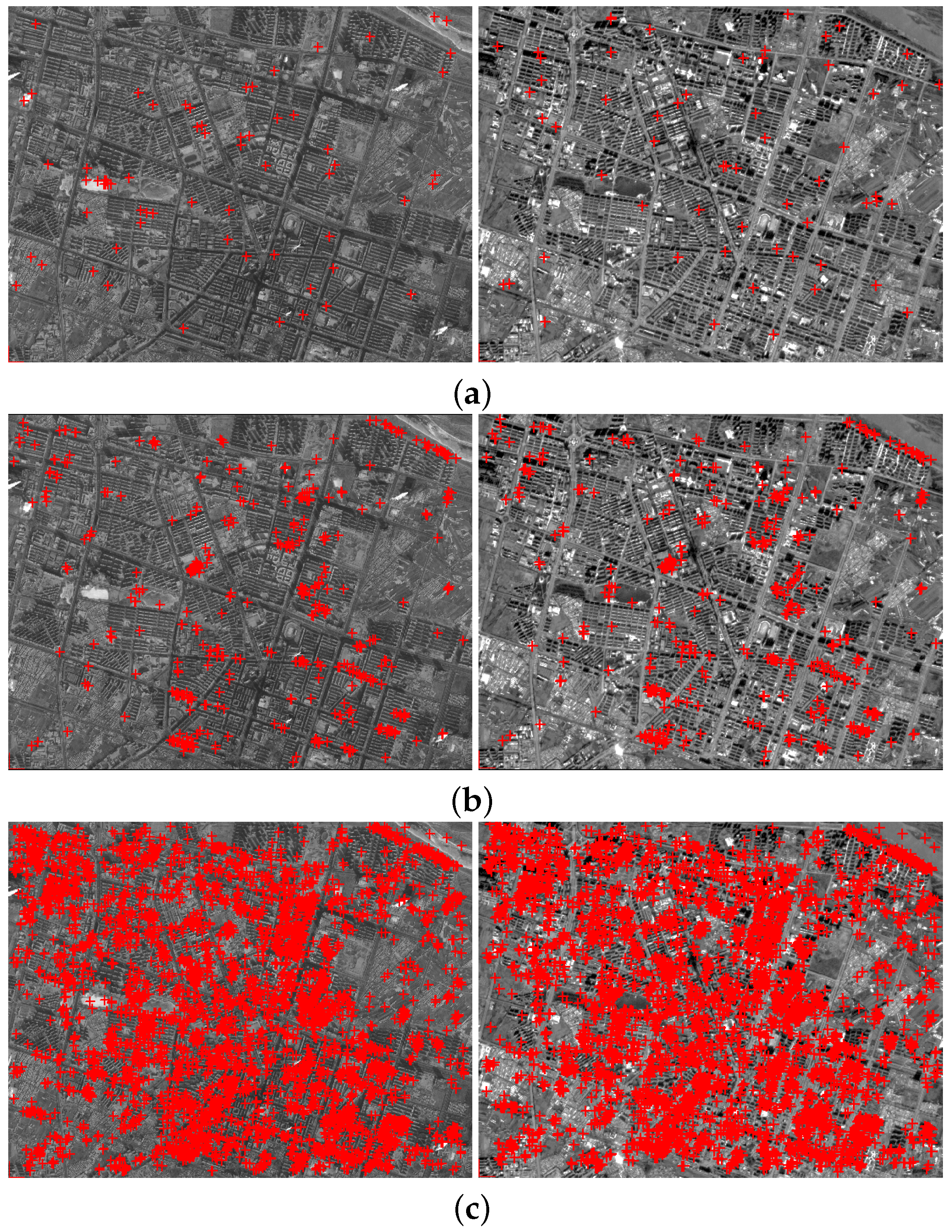
| TAACC | 3000 | 79 | 2.6% | 98.7% | 102.3 |
| GC | 3000 | 691 | 23.0% | 1.4% | 3.4 |
| Proposed method | 3000 | 1946 | 64.8% | 0.6% | 2.4 |
| Matching | Number of | Number of | Successful Rate | Mismatching | RMSE |
|---|---|---|---|---|---|
| Method | Interest Points | Matching Points | of Matching | Rate | (m) |
| TAACC | 26,044 | 11,672 | 44.8% | 8.4% | 10.3 |
| GC | 26,044 | 4985 | 19.1% | 1.8% | 6.2 |
| Proposed method | 26,044 | 19,617 | 75.3% | 0.8% | 5.0 |
© 2016 by the authors; licensee MDPI, Basel, Switzerland. This article is an open access article distributed under the terms and conditions of the Creative Commons Attribution (CC-BY) license (http://creativecommons.org/licenses/by/4.0/).
Share and Cite
Ling, X.; Zhang, Y.; Xiong, J.; Huang, X.; Chen, Z. An Image Matching Algorithm Integrating Global SRTM and Image Segmentation for Multi-Source Satellite Imagery. Remote Sens. 2016, 8, 672. https://0-doi-org.brum.beds.ac.uk/10.3390/rs8080672
Ling X, Zhang Y, Xiong J, Huang X, Chen Z. An Image Matching Algorithm Integrating Global SRTM and Image Segmentation for Multi-Source Satellite Imagery. Remote Sensing. 2016; 8(8):672. https://0-doi-org.brum.beds.ac.uk/10.3390/rs8080672
Chicago/Turabian StyleLing, Xiao, Yongjun Zhang, Jinxin Xiong, Xu Huang, and Zhipeng Chen. 2016. "An Image Matching Algorithm Integrating Global SRTM and Image Segmentation for Multi-Source Satellite Imagery" Remote Sensing 8, no. 8: 672. https://0-doi-org.brum.beds.ac.uk/10.3390/rs8080672