Interferometric SAR Coherence Models for Characterization of Hemiboreal Forests Using TanDEM-X Data

Abstract

In this study, four models describing the interferometric coherence of the forest vegetation layer are proposed and compared with the TanDEM-X data. Our focus is on developing tools for hemiboreal forest height estimation from single-pol interferometric SAR measurements, suitable for wide area forest mapping with limited a priori information. The multi-temporal set of 19 TanDEM-X interferometric pairs and the 90th percentile forest height maps are derived from Airborne LiDAR Scanning (ALS), covering an area of 2211 ha of forests over Estonia. Three semi-empirical models along with the Random Volume over Ground (RVoG) model are examined for applicable parameter ranges and model performance under various conditions for over 3000 forest stands. This study shows that all four models performed well in describing the relationship between forest height and interferometric coherence. Use of an advanced model with multiple parameters is not always justified when modeling the volume decorrelation in the boreal and hemiboreal forests. The proposed set of semi-empirical models, show higher robustness compared to a more advanced RVoG model under a range of seasonal and environmental conditions during data acquisition. We also examine the dynamic range of parameters that different models can take and propose optimal conditions for forest stand height inversion for operationally-feasible scenarios.

1. Introduction

Forest Above Ground Biomass (AGB) is a key variable in the assessment of the state of global forest resources and monitoring its change [1]. Forests are subject to a variety of disturbances, including deforestation, forest degradation, logging operations, forest regrowth and regeneration. Due to the essential role of forests in the global carbon cycle, uncertainties in the AGB estimation affect the accuracy of the carbon stock accounting and can lead to significant uncertainties in the model output. This requires development and implementation of reliable and robust AGB estimation and monitoring methods.

Ground-based inventories are often insufficient for providing frequent up-to-date information on the extent, spatial distribution and dynamics of forests covering vast areas. A more economical approach lies in systematic integration of Earth Observation data with high quality ground measurements. There exists a variety of methods for mapping forest biomass [2], most notably airborne [3] and spaceborne LiDAR (Light Detection And Ranging) scanning [4], satellite optical remote sensing [5] and space-borne imaging radar [6]. Airborne surveys, however, are relatively costly, while approaches using satellite optical data are often obscured by clouds and suffer from a lack of solar illumination, particularly in high latitudes. Furthermore, optical satellite data have limited value for forest biomass estimation, since the reflectance primarily originates from the upper layer of the forest canopy, and the vertical structure is not assessed. In this situation, using Synthetic Aperture Radar (SAR) satellite data might be the most practical option for large-scale forest mapping [7] by being a cost-effective and time-efficient way to obtain regular estimates of forest resources and to provide accurate input for carbon cycle models.

Two widely-known techniques for radar-based AGB estimation are: (1) direct interpretation of the backscattered SAR signal; and (2) radar-based forest height estimation combined with allometric relations. The first approach typically suffers from signal saturation [8], which renders the method unusable for high biomass forests. The saturation level is affected by wavelength, radar polarization, forest characteristics and environmental conditions during the image acquisition. Relationships between AGB and SAR backscatter can be both model-based and empirical. However, training data are typically necessary for this approach to be effective [9,10,11]. The second widely-adopted family of approaches uses interferometric SAR (InSAR) images to estimate forest height, which is an important forest variable. Furthermore, radargrammetry, a technique that relies on a reference ALS-based DTM, is giving promising results for potential applications in large-area boreal forest AGB mapping [12,13,14]. The radar estimated forest height can be applied for deriving aboveground forest biomass [15,16,17,18,19], canopy density [20], estimating carbon flux [21], detecting changes in forests [22] or improving the inventory data for remote areas [23].

Most InSAR techniques use coherence, which is a measure of the complex correlation between two SAR images, and it can be related to forest height using appropriate physics-based [24] or empirical relationships. Unfortunately, the estimation of forest height exclusively from interferometric coherence requires a fully-polarimetric measurement that is not routinely and widely available in the case of spaceborne SAR. Another important factor affecting the usability of InSAR coherence is the level of temporal decorrelation when image acquisitions are separated by a time interval. In the case of bistatic TanDEM-X single pass acquisitions, the latter factor can be neglected.

Supervised semi-empirical and empirical methods particularly using linear [19,25,26,27] and non-linear regression [26,27,28] and non-parametric models [23] are popular tools for relating InSAR coherence and forest parameters. Approaches relying on InSAR coherence magnitude (e.g., [19,26]) and phase (e.g., [23,27,28] in the presence of external DTM), as well as their combination (as suggested in [24]) were found useful in estimating forest variables. Promising results for model-based forest height estimation were demonstrated over a variety of frequency bands and sites from boreal [17,29,30,31] to tropical forests [32,33,34]. However, practically all of these studies were performed only over relatively small test sites and typically required auxiliary data.

Despite successful demonstrations of the potential sophisticated algorithms in several empirical studies, a framework for operational forest height retrieval has not yet been established. In the current work, we try to fill this gap and provide a set of simple, theoretically-justified models and associated methods for relating forest height to available single-polarization coherence data, particularly suitable for wide area (e.g., country-level) mapping. We consider the operational forest height inversion scenarios in the hemiboreal forest environment for enabling downstream services, using only coherence magnitude in absence of any other auxiliary information. Focus is on the coherence magnitude-based forest stand height retrieval, as phase inversion requires additional ground DEM, which is not available globally or is of poor quality. We investigate several simple models suitable for this inversion scenario subject to their suitability, robustness and adequacy of data description and determine the range of validity of these models and the dynamic range of their parameters. The influence of forest tree species is studied, as well, in order to determine if this aspect should be considered during forest height retrieval. Experimental data are represented by bistatic TanDEM-X acquisitions.

Firstly, we establish a simple theoretical framework based on the RVoG model and derive models with different complexity levels. We then investigate the performance of the proposed models by comparing the models with extensive multi-temporal coherence magnitude data acquired over Estonia. This is followed by defining the range of validity of these models for reliable inversion and assessing the inversion parameters for the feasible operational production scenario for three main forest types in the hemiboreal zone.

The paper is organized as follows. In Section 2, we discuss model-based approaches for forest height extraction from InSAR data and present the models examined in the study. Section 3 describes the study areas, TanDEM-X data and reference data used. Section 4 provides an overview of the data processing. Experimental results are presented and discussed in Section 5, and the article is concluded in Section 6.

2. Forest Parameter Relation with Interferometric SAR Measurement

2.1. Interferometric SAR Measurements of Forests

In the case of interferometric SAR (InSAR) measurement, the measured variable is coherence, which is the normalized complex cross-correlation between two complex signals (two SAR images, separated by a baseline) $s_1$ and $s_2$ and is defined as:

$$\gamma =\frac{〈s_1{s}_2^{*}〉}{\sqrt{〈s_1{s}_1^{*}〉〈s_2{s}_2^{*}〉}},0\le \left|\gamma \right|\le 1$$

(1)

where $\langle ..\rangle$ denotes an average over the ensemble of pixels, usually selected by a sliding window of size (azimuth × range) in a single look complex image. Interferometric coherence is essentially a complex variable, combining both the coherence magnitude and interferometric phase. In general, the measured coherence γ can be described as a product of the following factors:

$$\gamma ={\gamma }_{System}{\gamma }_{SNR}{\gamma }_{Temp}{\gamma }_{Vol}$$

(2)

where ${\gamma }_{System}$ combines decorrelation caused by measurement system quantization, ambiguities, relative shift of the Doppler spectra and the baseline, ${\gamma }_{SNR}$ describes the coherence decrease caused by the finite sensitivity of the system (the signal to noise ratio), ${\gamma }_{temp}$ accounts for changes in the target over time and ${\gamma }_{Vol}$ describes decorrelation caused by volume scattering over vegetated areas where several scatterers at different heights contribute to scattering [35]. The two last terms depend on target properties and have the largest dynamics when measuring natural targets.

Forest parameter estimation from InSAR measurements assumes that forest causes a decrease of coherence due to volume scattering (referred to as volume decorrelation) and can therefore be characterized by interpreting the coherence (1). The amount of decorrelation depends on the imaging configuration and also on the properties of the volume.

One of the most important descriptors of the volume is the thickness of the volume layer and the attenuation properties of the medium. As can be seen from (2), distinguishing between temporal and volume scattering-induced effects is difficult, and therefore, the measurement is arranged in a way that the temporal decorrelation can be neglected, for example by making measurements for both signals simultaneously.

2.2. RVoG Coherence Model

One of the simplest physics-based models describing volume scattering effects to InSAR coherence ${\gamma }_{Vol}$ is the Random Volume over Ground (RVoG) model. It relates the volume induced decorrelation ${\gamma }_{Vol}$ in observed interferometric coherence (1) to the physical properties (structure) of the forest layers [36,37,38]. RVoG is closely associated with the interferometric water cloud model [39], [24] and can be considered a simplified version of the latter when gaps in vegetation are excluded from the analysis [16].

The RVoG is a two-layer model that assumes that a homogeneous layer of volume scatterers, representing the forest canopy, is located over a reflective ground layer, while ignoring the even-bounce scattering mechanism and higher order interactions. The model has been used for retrieving forest parameters from polarimetric interferometric SAR data, which are able to provide a sufficient number of independent measurements. The RVoG model presents the interferometric coherence as a normalized sum of volume coherence ${\gamma }_V$ and the polarization ω-dependent ground reflection term $\mu \left(\omega \right)$ as:

$${\gamma }_{RVoG}=e^{i\varphi }\left(\frac{{\gamma }_V+\mu \left(\omega \right)}{1+\mu \left(\omega \right)}\right)$$

(3)

where the common ground phase is taken into account with the coefficient, reliant on the ground phase φ. The term ${\gamma }_V$ is dependent on both the volume layer properties and also on the imaging configuration. The equation (3) can also be presented in the form of:

$${\gamma }_{RVoG}=e^{i\varphi }\left(1-\frac{1-{\gamma }_V}{1+\mu \left(\omega \right)}\right)$$

(4)

where the variable μ occurs only once, as proposed in [31].

The volume decorrelation term ${\gamma }_V$ is the Fourier transform of the normalized scattering profile in the vertical direction. When assuming a random isotropic volume, the profile can be modeled with an exponential distribution and ${\gamma }_V$ can be written as:

$${\gamma }_V=\frac{{\int }_0^h{e}^{\sigma z}{e}^{i{\kappa }_{z}z}dz}{{\int }_0^h{e}^{\sigma z}dz}$$

(5)

where the parameter σ describes the attenuation in the volume layer and is called extinction, and imaging geometry is described by the vertical wavenumber ${\kappa }_z$. It is important to note that in this simplified notation, the extinction parameter σ depends also on the incidence angle θ because $\sigma =\frac{2{\sigma }_m}{cos\left(\theta \right)}$, where ${\sigma }_m$ is the extinction coefficient of the medium. After integration, one can write:

$${\gamma }_V=\frac{\sigma (e^{h\sigma }{e}^{i{\kappa }_{z}h}-1)}{(\sigma +i{\kappa }_z)(e^{h\sigma }-1)}$$

(6)

The RVoG model is obtained by combining Equations (6) and (3). The model depends on imaging geometry ${\kappa }_z$ and on three variables characterizing the volume: volume extinction σ, volume layer height h and the polarization-dependent term $\mu \left(\omega \right)$ that defines the contribution of the scattering from the ground. The model also depends on the SAR instrument wavelength via ${\kappa }_z$ and extinction, which is a function of wavelength.

As seen, the model connects forest height to measured interferometric coherence and provides the opportunity to derive the height directly from InSAR coherence. However, despite being a relatively simple approach, this model still has four unknown parameters and, therefore, needs at least four independent measurements for rigorous inversion. Therefore, at least two independent complex measurements are required for model inversion at the pixel level. Typically, fully-polarimetric SAR data are used to provide a sufficient amount of measurements to derive the coherence region and allow meaningful model inversion. However, such data are not routinely available from space. To overcome this difficulty and obtain height estimates using dual-polarization (dual-pol) or even single-polarization (single-pol) InSAR data [31,34], additional assumptions, auxiliary data or further regularization are needed. Including the auxiliary Digital Terrain Model (DTM) representing ground surface, fixing the phase center height location, discarding the ground scattering contribution and fixing the forest extinction to a predefined value are among the commonly-used solutions [31,33,34,40].

3. Simplified Coherence Models for Forests

The performance of a coherence model is influenced by several factors, such as the selection of the perpendicular baseline (affecting the vertical wavenumber) [34], the seasonal variability of the volume extinction and ground reflectance [41,42]. For example, the dependence of the model-based inversion on weather conditions has been studied to a very limited extent [43,44], and no studies focused on the peculiarities of forest height retrieval for different forest species. When working with space-borne coherence data, the quantity of independent measurements is usually limited, and various error sources cannot be entirely controlled. Therefore, in practice, often, simpler models than the RVoG are applied in order to retrieve forest height from coherence magnitude measurement. Despite its relative simplicity, the RVoG model is still too complicated for operational forest height estimation, and a variety of simplifications, such as regression models or the sinc model, are typically used. Moreover, practically all pf the above-mentioned studies using RVoG were carried out over relatively small test sites (at the extent of one scene), typically with a specific dominating type of forest. Wide area mapping, however, requires a somewhat different, more robust approach, which would allow model inversion based on available single-polarization data. Reliable inversion is needed over all service areas, and a set of applicable models and the dynamic range of their parameters should be well defined for different inversion scenarios. A regression model cannot answer to those demands, and in the following, we propose an RVoG model simplification to provide a set of semi-empirical models to form a physics-based framework for coherence modeling for forest height retrieval.

3.1. RVoG Model Simplifications

As was noted above, simpler models have several benefits during practical forest height retrieval, mainly in terms of invertibility. One straightforward way to simplify the RVoG model is to eliminate some of its variables. This can be, for example, done by considering the volume decorrelation integral (5) in the case where extinction parameter σ approaches zero. The $\sigma =0$ condition should be applied prior to the integration in order to derive a defined function. Effectively, this means that the profile function in (5) is assumed to be constant instead of exponential. The simplification can be derived in the form of:

$${\gamma }_{V0}=\frac{(e^{ih{\kappa }_z}-1)}{ih{\kappa }_z}$$

(7)

This can be presented using trigonometric functions as:

$${\gamma }_{V0}=e^{i\frac{h{\kappa }_z}{2}}\frac{sin\left(\frac{h{\kappa }_z}{2}\right)}{\frac{h{\kappa }_z}{2}}=e^{i\frac{h{\kappa }_z}{2}}sinc\left(\frac{h{\kappa }_z}{2}\right)$$

(8)

which provides the equation as a product of the imaginary and real functions [45]. As can be noted from (7) and (8), a convenient argument for this problem is not h, but $h{\kappa }_z$. Moreover, when taking into account the definition of InSAR height of ambiguity, defined as:

$$HoA=\frac{\lambda R_D\sin \left(\theta \right)}{2\pi LN}=\frac{2\pi }{{\kappa }_z}$$

(9)

where λ is the wavelength, θ is incidence angle, L is baseline, $R_D$ is the range distance, $N=2$ denotes monostatic and $N=1$ for bistatic measurement and ${\kappa }_z$ is the vertical wavenumber, the zero extinction volume decorrelation can be presented as:

$${\gamma }_{V0}=\frac{i}{2\pi }\left(1-e^{i2\pi \frac{h}{HoA}}\right)\frac{HoA}{h}=e^{i\pi \frac{h}{HoA}}sinc\left(\pi \frac{h}{HoA}\right)$$

(10)

Here, the $\frac{h}{HoA}$ can be interpreted as a relative (fringe-height-normalized) height of the forest stand. The $\frac{h}{HoA}$ is a dimensionless parameter, which provides comparable reference for volume-induced coherence, measured with different baselines.

When substituting the simplified volume decorrelation function (10) into RVoG model (3) and assuming zero ground contribution $\mu =0$, the so-called sinc-model can be derived as:

$$|{\gamma }_{sinc}|=sinc\left(\pi \frac{h}{HoA}\right)$$

(11)

A particular benefit of the sinc model is that it can be used for coherence magnitude-based inversion [31,43,44] or, alternatively, in hybrid inversion scenarios where both the magnitude and the phase of the InSAR coherence are used [24]. The drawback is that it is harder to explain model performance in the typical terms in which the RVoG operates, i.e., ground-to-volume ratio and extinction. Furthermore, the simple sinc model does not take into account the interferometric phase.

3.2. Linear Model for Coherence

An even simpler model can be constructed using the RVoG model to establish a linear relation between coherence and forest height. The motivation for that is given by the fact that often, a linear relation between forest height and interferometric coherence is established empirically. This can be done using linear approximation for the sinc function. It is known that for height estimation with the RVoG model, the forest height should generally be in the range, or smaller, than the height of ambiguity. This means that the argument range of (11) is restricted to an area between zero and π. In this region, the sinc function can be approximated rather well with a simple linear function $(1-\frac{x}{\pi })$. By replacing the sinc in (10) with this linear function, one can derive a simple linear approximation for the coherence and height relation as:

$${\gamma }_l=e^{i\varphi }{e}^{i\pi \frac{h}{HoA}}\left(1-\frac{h}{HoA}\right)$$

(12)

where h denotes the thickness of forest volume (forest height), HoA is the Height of Ambiguity of the SAR system and φ is the interferometric phase on the ground. When only the coherence magnitude is considered, the above model (12) represents a simple linear relationship between the volume height and InSAR coherence and shows that the RVoG model can be used to explain theobserved linear relationship between the forest height and interferometric coherence amplitude.

It will be demonstrated later that when plotting $\frac{h}{HoA}$ against coherence values, the result depends on the imaging configuration much less than on the actual forest stand height. Therefore, in the following, we will use $\frac{h}{HoA}$ as an argument for empirical models.

3.3. RVoG-Based Semi-Empirical Models

In the following, we assume that the derived simplifications of the RVoG model capture the essential dependencies between the forest height, imaging parameters and the interferometric coherence. We assume that with additional empirical parametrization, the models can provide viable robust tools for forest height derivation from coherence images. However, in this work, we only investigate the plausibility of such models by comparing various possible models with ALS forest height and TanDEM-X coherence magnitude measurements. Here, we propose three semi-empirical models (13), (14) and (15):

$$|{\gamma }_{linear}|=1-\frac{h}{HoA}{C}_{lin}$$

(13)

$$|{\gamma }_{sinc}|=0.95·sinc\left(C_{sinc}\pi \frac{h}{HoA}\right)$$

(14)

$${\gamma }_{0ext}=\left[\left(1-e^{i2.4\pi \frac{h}{HoA}}\right)\frac{HoA}{h}\frac{i}{2.4\pi }-1\right]\frac{1}{C_{0ext}}+0.95$$

(15)

where $C_{lin}$, $C_{sinc}$ and $C_{0ext}$ are empirical parameters for the derived models. The linear model (13) is based on (12); the sinc-model (14) is based on (11); and the 0ext model (15) is derived by combining (7) with (4). The last model can be presented and constructed also in terms of a sinc function, but it is important to include both the imaginary and real components of the model for additional empirical parametrization. The magnitude of the model depends also on the imaginary component, and a simple real sinc model fails to agree with the data. There are also many more ways to parametrize (10) and get good empirical models. The parametrization here is performed in a way that keeps the shape of the original functions, but allows one to adjust slightly the model range to fit with the data. The models also contain a few constants, which are selected to adjust the model shape to meet the majority of the data. 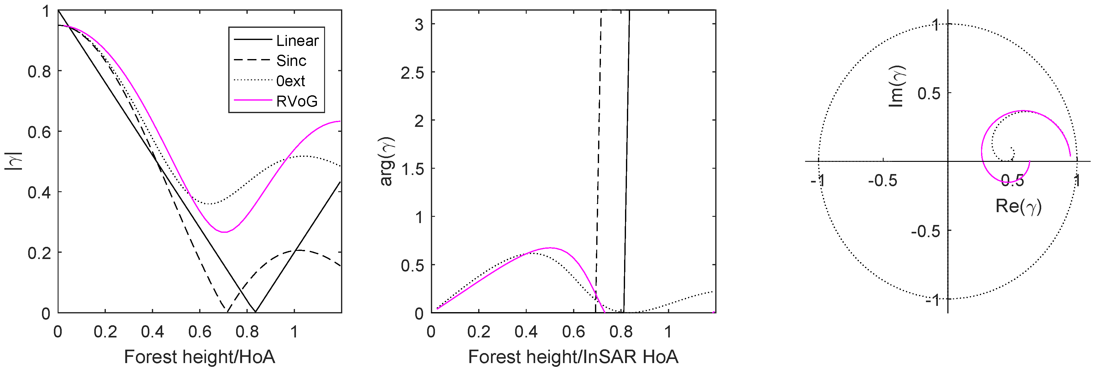For example, the coherence maximum is adjusted to a lower value than one (0.95 was selected according to the $0ext$ model fit to the entire dataset). The models are depicted graphically in Figure 1, where the general shape of the functions can be seen. As can be noted, all proposed models behave in a similar way for a coherence magnitude range of 0.4–0.8. Furthermore, linear and sinc models do not describe the phase, as they use only real functions. It has to be noted that the linear, sinc and 0ext model shapes do not contain additional dependencies on the baseline when the $h/HoA$ argument is used, but, the RVoG model has a more complex dependence on HoA; and the model shape is actually slightly different for different baselines also in the $h/HoA$ axis reference.

In the following, we proceed to assess the potential of the proposed models for forest height retrieval and define the applicable region of model parameters by using an extensive dataset of X-band multitemporal coherence magnitude images and ALS-based forest height maps.

4. Test Sites and Description of the Data

4.1. Study Area

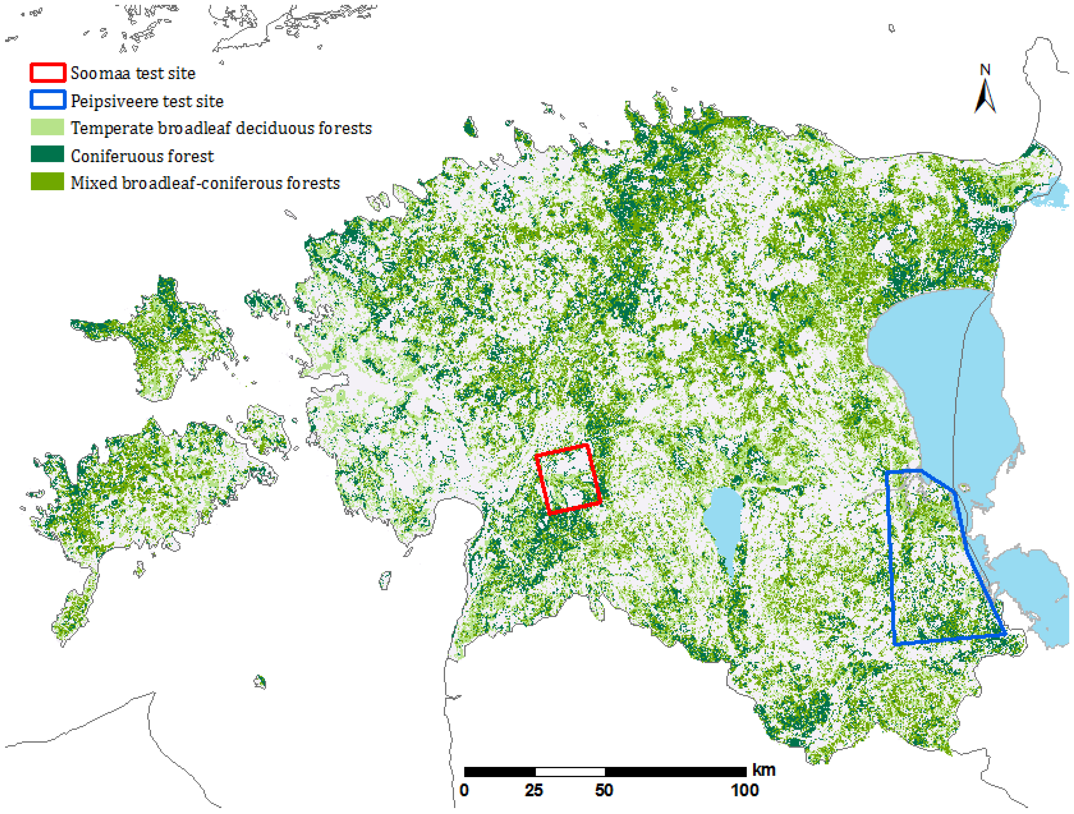
The study areas are located in southern Estonia (Figure 2). The first test site (12 km × 15 km) is situated in Soomaa National Park in southwestern Estonia ($58°{24}^{\prime }$N, $25°6^{\prime }$E), and the second Peipsiveere test site covered a larger region (46 km × 61 km) in southeastern Estonia ($58°8^{\prime }$N, $27°{19}^{\prime }$E). It is located in Tartu and Põlva County and includes the Peipsiveere Nature Reserve and the old-growth forests of the Järvselja Primeval Forest Reserve.

The Soomaa site is situated on a flat terrain (elevations ranging from 20–30 m above sea level) between large mires and rivers of the Pärnu River basin (Halliste, Raudna and Lemmjõgi). The Peipsiveere site contains the primeval forests of Järvselja Nature Reserve and Peipsiveere Nature Reserve that are located around the estuary of the Emajõgi River on the southwestern coast of Lake Peipus. The region is relatively flat (30–40 m above sea level) and surrounded by wetlands and forest.

As demonstrated in Figure 2, the forest data from the Estonian Forest Registry [46] are divided into three main classes according to the dominant tree species. A total of 242 forest stands covering 591 hectares of forests were selected over the Soomaa site, with the average stand size of 2.44 ha. The dominating tree species for more than half of the forests (116 stands) is Scots pine (Pinus sylvestris L.). The deciduous stands are represented by 101 stands, dominated by silver birch (Betula pendula Roth) with 57 stands and followed by black alder (Alnus glutinosa L.) with 36 stands, grey alder (Alnus incana L.) with five stands and trembling aspen (Populus tremula L.) with three stands. Norway spruce (Picea abies L.) has the smallest presence with a total of 25 stands.

The Peipsiveere site includes 563 forest stands covering over 1620 ha. The average stand size is 2.88 ha. The site conditions are influenced by the large wetlands and are also reflected in the distribution of the tree species common for wet locations and moist soils. The majority of the forests are deciduous (333 stands), composed of 303 silver birch and 26 black alder stands. The remaining four stands are represented by grey alder, larch (Larix decidua) Mill.) and aspen stands. The Scots pine forests include altogether 173 stands, while the smallest class is Norway spruce with 57 stands.

4.2. Forest Inventory Data

The forest inventory data were provided by the Estonian Environment Information Centre [46]. The data were used to select forest sub-compartments from the State Forest Registry for accounting of forest resources, which are integrated, sufficiently homogeneous in their origin, composition, age, basal area, height, standing volume and site type and subject to common methods of management [47].

The average stand height over the Soomaa test site is 16.7 m, with the stand height ranging from 1.4 m–29.7 m. The mean standing volume density over the test site is 140 ${\mathrm{m}}^3$/ha, ranging between 1 and 327 ${\mathrm{m}}^3$/ha. For the Peipisveere test site, the mean stand height is 14.8 m, with the stand height ranging from 1.5 m–30.2 m. The mean standing volume density over the test site is 121 ${\mathrm{m}}^3$/ha, ranging between 0 and 449 ${\mathrm{m}}^3$/ha.

The mean size of the 242 Soomaa stands is 2.44 ha (median 1.70 ha), ranging from 1.0 ha–15.2 ha. The mean size of the 563 Peipsiveere stands is 2.88 ha (median 1.96 ha), where the smallest stand is 1.0 ha and the largest 47.0 ha.

4.3. TanDEM-X Dataset

The interferometric SAR dataset consists of 19 TanDEM-X bistatic Stripmap (SM) dual polarization (HH/VV) and single polarization (HH) images acquired from 2010–2012 over the Soomaa (

Table 1. The list of bistatic TanDEM-X stripmap acquisitions over the Soomaa test site. HoA is the Height of Ambiguity.

ID	Date	Incidence Angle (°)	HoA (m)	Minimum Ground Temperature (°C)	Temperature (°C)	Precipitation (mm)	Polarization	Water Level (cm)	Orbit	Resolution Ground Azimuth/Range (m)	Pixel Spacing Ground Azimuth/Range (m)
1	29 December 2010	44.6	41.4	−9.2	−6.8	0	HH	112	Ascending	3.30/2.52	1.99/1.94
2	1 August 2011	36.2	45.9	12.0	18.6	0	HH	46	Ascending	3.30/2.99	2.04/2.31
3	3 March 2012	23.4	44.7	−5.3	0.9	0	HH/VV	88	Ascending	6.60/2.96	2.35/2.29
4	8 March 2012	34.8	66.2	−22.9	−2.7	0	HH/VV	81	Ascending	6.60/2.06	2.85/1.59
5	14 March 2012	23.4	43.6	−5.5	−0.4	0	HH/VV	91	Ascending	6.60/2.96	2.35/2.29
6	25 March 2012	23.4	43.9	−3.5	0.9	9.9	HH/VV	374	Ascending	6.60/2.96	2.35/2.29
7	5 April 2012	23.4	16.2	−8.4	4.6	0	HH/VV	258	Ascending	6.60/2.97	2.35/2.30
8	5 April 2012	18.2	41.8	−8.4	−3.7	0	HH/VV	271	Descending	6.60/3.76	2.8/2.94
9	15 April 2012	45.2	30.8	−2	10.8	0	HH	147	Ascending	3.30/2.49	2.01/1.92
10	02 May 2012	34.8	24.7	−2.2	13.4	0	HH/VV	122	Ascending	6.60/2.06	2.85/1.59
11	18 May 2012	43.4	32.7	6.5	12.3	11	HH	81	Ascending	3.30/2.57	1.85/1.98
12	30 May 2012	23.4	18.5	6.6	9.1	20.6	HH/VV	57	Ascending	6.60/2.97	2.35/2.31
13	3 October 2012	34.8	33.7	5.6	10.2	0	HH/VV	88	Ascending	6.60/2.06	2.85/1.59
14	11 November 2012	23.3	19.7	−0.2	5.1	0	HH/VV	234	Ascending	6.60/2.97	2.35/2.30
15	16 November 2012	34.8	31.8	0.6	5.5	0	HH/VV	174	Ascending	6.60/2.06	2.85/1.59

) and Peipsiveere test sites (

Table 2. The list of bistatic TanDEM-X stripmap acquisitions over the Peipsiveere test site.

ID	Date	Incidence Angle (°)	HoA (m)	Minimum Ground Temperature (°C)	Temperature (°C)	Precipitation (mm)	Polarization	Orbit	Resolution Ground Azimuth/Range (m)	Pixel Spacing Ground Azimuth/Range (m)
16	4 January 2011	44.6	41.6	-13.4	-5.2	2.2	HH	Asc	3.30/2.51	1.99/1.94
17	9 September 2011	36.2	48.2	7.3	13.7	0.8	HH	Asc	3.30/2.99	2.20/2.31
18	30 March 2012	45.2	30.1	0.0	1.6	3.1	HH	Asc	3.30/2.49	2.01/1.92
19	5 November 2012	43.4	33.6	1.6	2.7	12.6	HH	Asc	3.30/2.57	1.85/1.98

). In order to have a consistent dataset, only the HH-polarization component of dual-pol TanDEM-X Coregistered Single look Slant range Complex (CoSSC) scenes is used. As was demonstrated in our earlier study [44], there is typically a small difference between HH and VV polarizations due to a weak double-bounce mechanism as a result of the forest floor conditions and flat terrain. The VV polarization should mainly be considered when dealing with flooded environments, as inundated forest floor is better seen in the HH channel and has less impact on the VV channel coherence [44,48,49].

The images for Soomaa and Peipsiveere sites were acquired with effective baselines ranging from 64–259 m and incidence angles ranging from 18°–45°. The satellite look direction is to the right for all images. The minimum ground temperature in Table 1 and Table 2 shows the lowest ground temperature over a 24-h period, while the precipitation information is the sum of total rainfall over 24 h prior to the satellite data acquisition. Data in the temperature column were recorded in the nearest weather station [50] and reflect weather conditions during the data acquisition. The given water level in Table 1 is measured from the Halliste River and is relative to a long-term minimum [50].

4.4. ALS Data

Airborne LiDAR scanning (ALS) measurements over both test sites were carried out by the Estonian Land Board in June 2010 using a Leica ALS50-II scanner. The ALS data point density is 0.45 per ${\mathrm{m}}^2$ with a pulse repetition frequency of 94 kHz MPiA (multiple pulses in air).

The 90th percentile ($P_{90}$) of the point cloud height is used as an estimate of the forest height. The $P_{90}$ was chosen as it is known to have a strong linear correlation to the measured forest height [51]. The point heights above ground are calculated using a Digital Terrain Model (DTM) in the L-EST reference coordinate system. Data from 2659 forest stands are used for the analysis. The stand polygon shapes are buffered 20 m inside for the Soomaa test site and 15 m inside for the Peipsiveere test site to avoid the influence of the borderline errors and to take into account the sliding window footprint on the ground in coherence magnitude calculations. For each stand, ALS point clouds are then extracted and processed using FUSION/LDV freeware [52].

5. Data Processing

The processing steps of the TanDEM-X Coregistered Single look Slant range Complex (CoSSC) product include coherence calculation according to (1) with a sliding window of (azimuth×range) and orthorectification of the coherence product (range Doppler terrain correction and geocoding) using satellite orbital information and Ground Control Points (GCP) from the image metadata. SRTM DEM is used in connection with the orthorectification.

For the Soomaa test site, coherence values are calculated for CoSSC images according to (1) using window sizes (azimuth × range) of 12 × 21, 13 × 14 and 17 × 18 pixels. In the Peipsiveere area, the window sizes are 12 × 13 and 13 × 14 pixels. The coherence calculation window size projected to the ground is approximately squared, with the length of its shortest edge starting from 25 m and ranging to 45 m for the largest window. The use of a relatively large averaging window during coherence calculation guarantees that the coherence overestimation bias is always less than 0.02 [53] and, thus, insignificant.

Further, coherence magnitude images are imported into a GIS program and converted to the same reference coordinate system as the previously-calculated ALS measured forest height data and the stand borders from the forest inventory database. Forest stands are divided into three groups by the dominant tree species, and statistics were calculated for each stand, resulting in a corresponding mean coherence magnitude and mean ALS forest height.

In order to provide representative and less biased estimates of coherence and heights in model fitting, the coherence data are analyzed stand-wise using a stand border map from ancillary data. The features of the stand border map are buffered 20 m inside for the Soomaa test site and 15 m inside for the Peipsiveere test site, with the purpose of avoiding border effects during the coherence calculation. The buffer distance size is approximately half of the size of the coherence image pixel size. The values of coherence and stand height pixels are then averaged inside the buffered polygons for the stand-wise estimates.

Additional criteria for the selection of the forest stands is based on the size and composition of the main tree layer. From the remaining polygons, only stands larger than one hectare are included in the analysis. Furthermore, only homogeneous stands with one tree layer and no understory layer are selected with the requirement that the proportion of the dominant tree species in the main tree layer is higher than 75%.

From the ALS data, mean forest height is calculated for every forest stand using the 90 percentile ($P_{90}$) height above the ground values of all of the echoes. The ALS data were acquired during 2010, while TanDEM-X scenes were acquired during 2010–2012; this factor can potentially introduce minor height differences during the model fitting. As the growth speed of forest depends on many environmental variables, such as the age of the forest, site type and water access, the corresponding change in stand height (different also for every scene) is neglected.

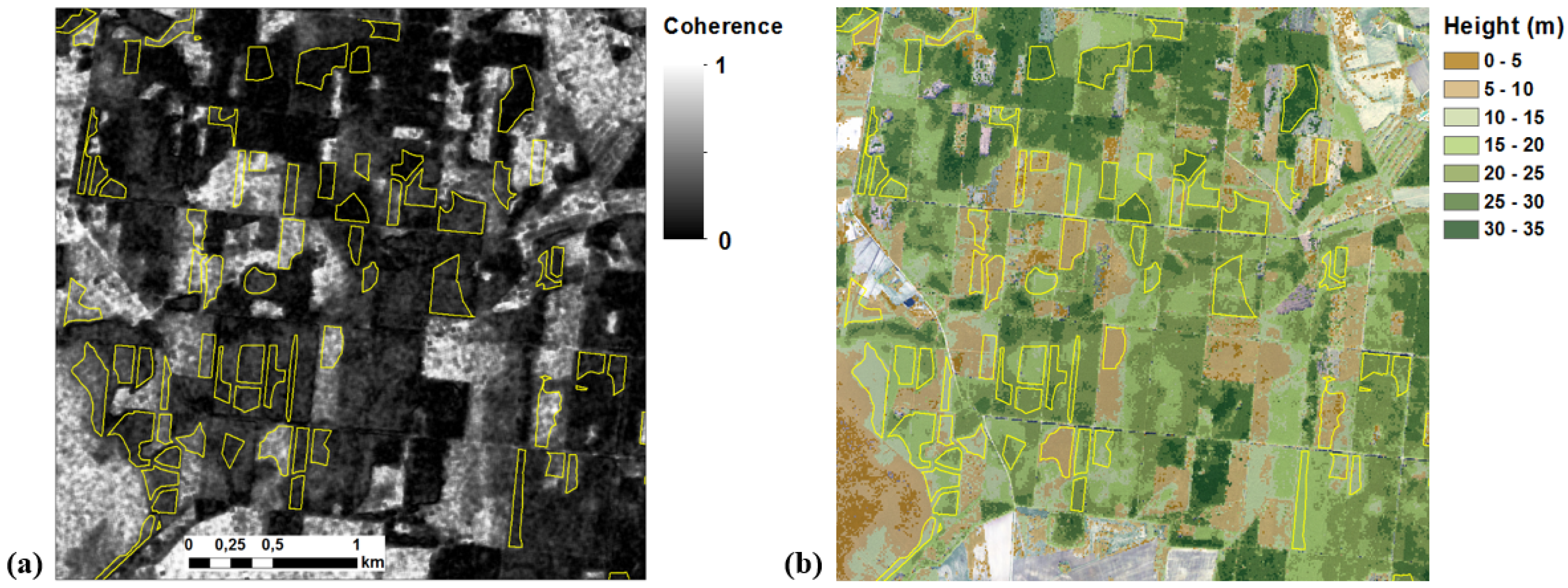
The pre-selected forest stands define the buffered polygons in which the coherence and ALS data are averaged and compared to each other, allowing one to calculate statistics for each forest stand. Figure 3 shows the TanDEM-X coherence magnitude image with the corresponding LiDAR-derived forest stand height map.

Fitting the Models to Measurements and Estimating Model Parameters

In the following section, three semi-empirical models (13), (14) and (15), along with the RVoG model (6) and (3) are compared using experimental data in order to evaluate their performance and to give estimates of the parameters of the models. The analysis is done by comparing stand-wise coherence magnitude measurements to the ALS measured stand average forest height data for every interferometric coherence image. Every coherence magnitude image contains a varying number of forest stands and has different imaging parameters. We assume that during the same acquisition, forests with a similar species composition have comparable attenuation and ground reflectivity properties and, therefore, can be described with the same model parameter.

Clearly, such an assumption works best only for relatively homogeneous forests. Here, we use forest dominant species to assure forest similarity.

A map of forest species is the most common and often the only a priori information available, thus also suitable for the operational scenarios. Therefore, three dominant tree species (pine-dominated, spruce-dominated and deciduous forests) are analyzed separately in the study areas. All four presented models are fitted to the data in order to find the best parameter values and the goodness of fit. The model-fitting is performed separately for every scene and dominant species class. Parameter values are found by using an unconstrained non-linear optimization (Nelder–Mead method) to seek the minimum difference between the forward modeled coherence magnitude and the ALS forest height in the least squares sense. The goodness of fit is calculated as the root-mean-square deviation between the measured coherence magnitude and modeled coherence for the current subset as:

$$RMSD=\sqrt{\frac{{\sum }_{i=1}^N{\left(x_i-x_i^{meas}\right)}^2}{N}}$$

(16)

where $x_i$ and $x_i^{meas}$ are the modeled and measured coherence magnitudes for the i-th forest stand and N is the number of examined stands (either whole scene or specific forest type).

6. Experimental Results

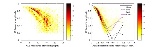
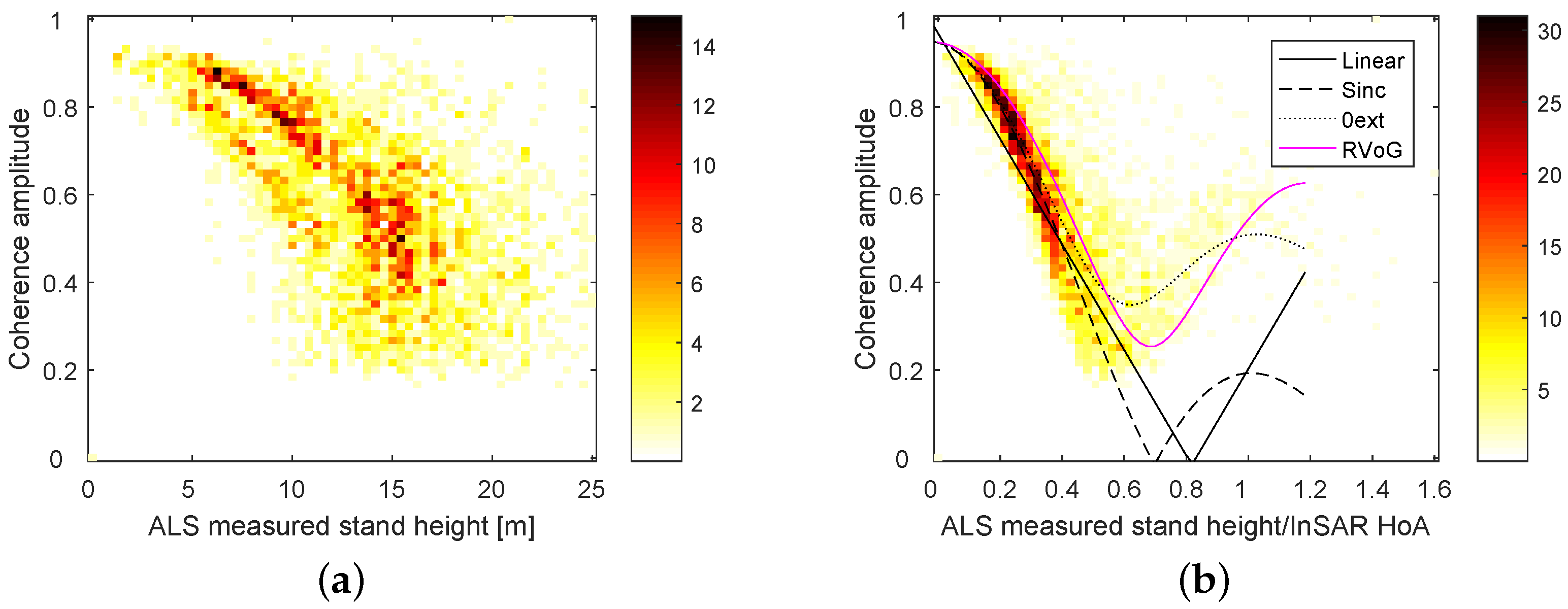
In Figure 4, an overview of the entire multitemporal dataset is presented as a relation between the coherence magnitude and ALS forest height. The dataset comprises 3787 forest stands on 19 different image pairs acquired over two years. The left image shows the initial relation between forest stand heights and coherences, and on the right side, the same relation corrected with HoA (9) is shown. The benefit of using $h/HoA$ as an argument is apparent, as the the variability caused by different baselines is mostly eliminated. For comparison, all three proposed semi-empirical models are presented on top of the data. Here, for simplicity, only one RVoG line is shown, while in reality, RVoG has slightly different curves for every baseline. As can be seen, at the general level, all models provide a reasonably good agreement with the majority of the measurements. However, it can be noted that the linear and sinc models cannot account for the ground contribution and assume zero coherence on the ground. On the other hand, it is remarkable how closely most of the measurements are located to a single line, taking into account that the graph covers all seasonal differences of three different forest types and several baseline configurations. In the following, a more detailed comparison between the models and data is provided scene by scene.

6.1. Model Performance across Different Scenes

Relationships between the ALS measured stand height and coherence magnitude estimates are presented in Figure 5 for individual interferometric scenes and dominant tree species, along with the results of fitting the four proposed coherence models to the data. Only a selection of five representative images (out of 19 scenes in total) are shown in the figure.

All forest scenes generally exhibit a similar behavior with respect to the measured coherence in the $h/HoA$ coordinates. Furthermore, all four models show agreement with the data, especially when the coherence is in the range between 0.4 and 0.9. In some cases, a very good correlation can be observed (particularly the 4 January 2011 and 3–25 March 2012 scenes) down to as low a coherence as $0.2$.

The dominant species of the forest has an effect on the model parameters. For example, the scene acquired on 30 March 2012 shows that deciduous forest had clearly different extinction properties compared to coniferous forests. On the other hand, it appears that differences in between acquisition dates are larger than differences between tree species.

One notable feature that can be observed is that the negative correlation between forest height and coherence magnitude can turn into a positive correlation when the stand height is close to HoA (or even exceeds the HoA value), as for example seen on the 5 April 2012 or 30 March 2012 scene. This indicates that potential inversion based on the proposed models might still be possible even when the forest height exceeded HoA. However, errors are large, and potential inversion could lead to ambiguous results.

The different models mostly agree in the region of $0.2<h/HoA<0.6$. However, it can be clearly seen that in the case of high coherence magnitude values (>0.9), the linear model is not adequate and fails to describe the data, while all other models agree well with each other and with the data. The differences between the sinc model and the RVoG model become evident in the case of low coherence values where RVoG and the 0ext model adapt well to variations in the attenuation and ground reflection strength. A good compromise between the RVoG model and the sinc model appears to be the 0ext model, which is a single parameter model like the sinc model, but allows flexibility close to that of RVoG. While the RVoG model adapts clearly best for all of the cases, this might have no importance in the operational scenarios where model parameters are unknown and the model flexibility hampers the potential inversion process. Therefore, for an operational height retrieval scenario, the linear model and the 0ext model might give the best results, as the 0ext model is more stable for small changes than RVoG, which has very high sensitivity for some combinations of ground to volume ratio and extinction.

According to RVoG, stands with high extinction and/or very strong ground contribution should occupy the region in the plot with high $h/HoA$ and high coherence magnitude values. However, there are only a few such data points in our dataset, and presumably, such parameter combinations are not common for hemiboreal forest in the case of the X-band.

6.2. Goodness of Fit for Different Models and Tree Species

Different forest stands are likely to have slightly different extinction and ground reflectivity values, partially explaining fit error and scatter in the data, as a single model explains only the variation of heights between different forest stands. The variations in the ground contribution tend to increase the coherence magnitude and scatter the data towards the “tail” of RVoG. In other words, the coherence magnitude for a certain forest height can be significantly higher than expected, but very seldom lower than a certain limit. Therefore, when solving an inverse problem, it should be taken into account that the coherence model errors are asymmetric and tend to scatter towards higher coherence magnitude values.

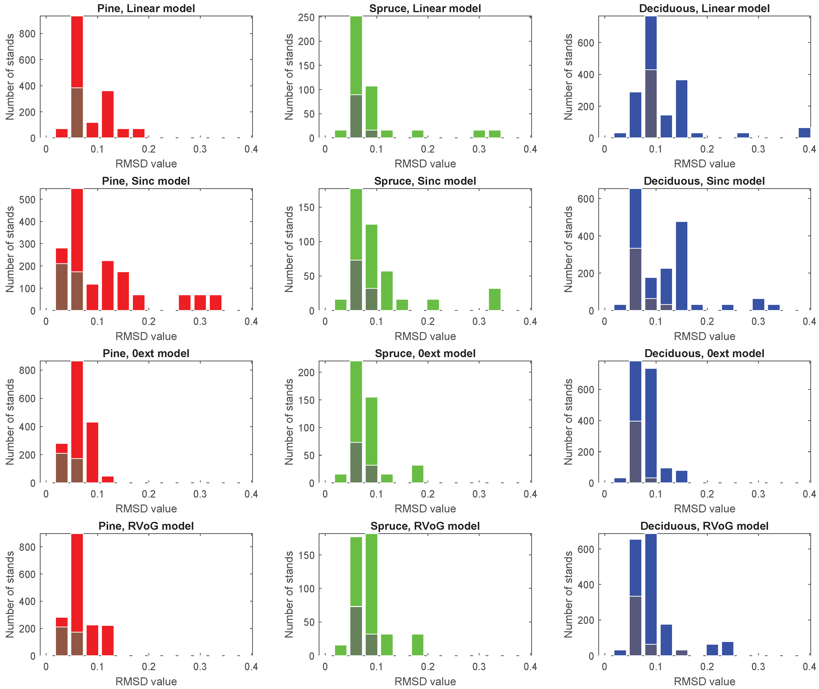
Figure 6 illustrates the goodness of fit for three forest types across all stands and InSAR scenes for the examined models using the RMSD measure where the 0ext model shows the best performance. Every stand is accounted in the histograms as a separate data point despite the fact that stands from the same scene have identical values for model parameters. As can be seen in Figure 6 (top row), the linear model has higher minimal error, but agrees rather well with a variety of the data. It cannot describe data well in the case of low coherence magnitude values and also has a significant deviation for coherence values above 0.9 (see Figure 5). The biggest drawback of using the linear model is that it cannot describe the increase of coherence magnitude (in response to increasing $h/HoA$) upon reaching intermediate values, like in the case of the 30 March 2012 scene (the “tail” scenario).

The same problem hampers the performance of the sinc model, which seems to offer slightly better performance than the linear model when the coherence is relatively high, but conditions present on the 30 March 2012 scene are problematic to describe. The sinc model has the poorest fit with the data in the region where stand height is closer to the height of ambiguity.

Based on the goodness of fit, the best performance is provided by the 0ext model and RVoG. On average, the 0ext model performs similarly to or even better than RVoG. A possible explanation is related to the high robustness of the 0ext model. In cases where the RVoG parameters take extreme values to fit the coherence magnitude points in the low coherence region, the 0ext model behaves in a more robust way. On the other hand, RVoG provides the best fit for scenarios when coherence values start to increase with increasing $h/HoA$ (e.g., the 30 March 2012 scene), something that is not captured by other models.

The pine-dominated stands show the best agreement with the elaborated models. This is probably due to the homogeneity and similarity between the stands. Therefore, the pine stands agree best with the general assumptions made about the similarity between the stands on one image.

6.3. Goodness of Fit for Different Baselines

During the analysis, it was noted that the RMSD values are correlated between the different models, probably indicating the limitations of the assumption of similarity between stands from the same stratum. When the extinction values or ground contribution of the stands are in reality very different, a single model line cannot fit all of the points.

The dependence of the model fitting error on HoA is shown in Figure 7. The HoA appears to be one of the main parameters influencing the goodness of fit. There is a strong dependence between the linear and sinc model fitting error and HoA, which is caused mainly by the fact that these models are not able to adapt to the “tail” scenario (see Section 6.2). A similar dependence is visible for the more complex models, but to a lesser extent. One should keep in mind that the RMSD of the coherence magnitude model fit does not directly describe the error of the stand height accuracy, as both depend on HoA in a similar way. Therefore, the most accurate forest height predictions would be possible in cases where HoA is small enough to enable large coherence dynamics, but large enough to avoid the effects caused by true height being close to the HoA. The scenes with HoA around two-times higher than the stand height appear to be an optimal choice for forest height inversion. This is in good agreement with, e.g., [42] where it was observed that for Norway spruce-dominated forest with maximum tree heights of about 30 m, the optimum HoA is in the range of 20–50 m.

6.4. Goodness of Fit for Winter Scenes

In Figure 6, the darker bars in all plots depict a subset of the data with frozen conditions. The subset comprises five scenes (4 January 2011, 3 March 2012, 8 March 2012, 14 March 2012, 25 March 2012), where the temperature has been significantly below the freezing point throughout the day. For all of those images, the HoA is approximately two-times higher than the highest stand height. Those conditions seem to give the best fit with models and create also the most favorable conditions for model inversion. It is notable that these scenes give a similar error level throughout all of the models, including the simple linear model. These results indicate the potential feasibility for forest height retrieval using single-pol X-band data and simple models given certain acquisition conditions. This is supported by the results from [42], where, based on the evaluation of InSAR height dynamics within the forest canopy, scenes acquired either only in frozen or only in unfrozen conditions are recommended for forest parameter estimation.

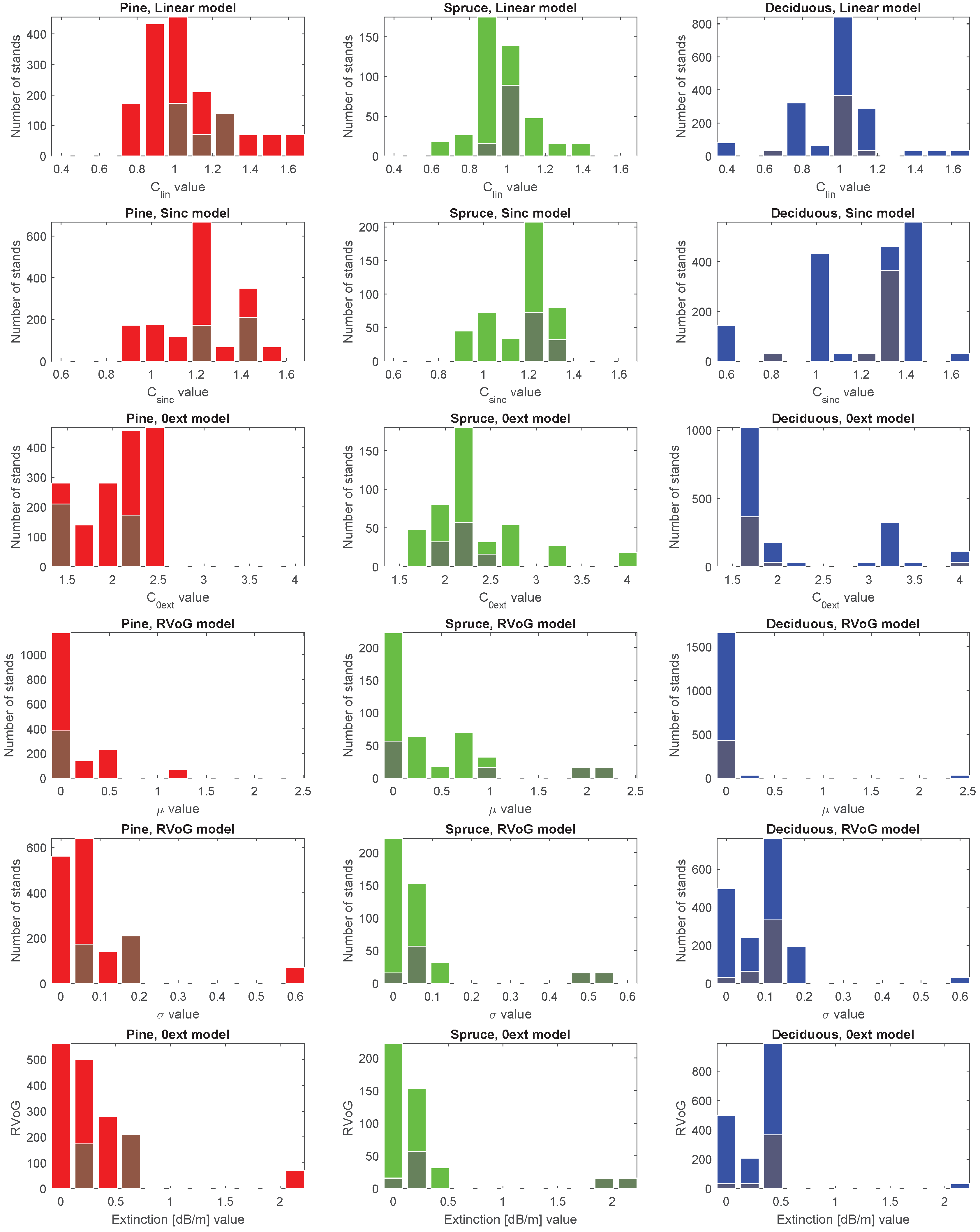
6.5. Parameter Range for Different Models

Figure 8 illustrates the species-wise dynamic range of parameters that the chosen models take across all InSAR scenes. Every stand is again counted as one data point in the histogram. The best fitting winter scenes are highlighted with darker bars. In general, differences between tree species are small. Larger variability and a smaller sample of spruce-dominated and deciduous stands has led to a wider variability in most of the parameters, respectively.

It should be taken into account that in the case of a poor fit, the model parameters tend to find middle ground and do not tell much about the target. Therefore, it is interesting to look at the results from the winter scenes, highlighted with darker bars. These describe parameter values for cases where the noise is the smallest. Interestingly, the parameters for pine stands show different regions where the model fit is good, indicating that the forest attenuation properties and/or ground contribution are clearly different for different acquisition dates.

From the linear model, it is easy to demonstrate the influence of the chosen parameter $C_{lin}$ value on height prediction accuracy. With coherence magnitude around $\gamma =0.5$, a variation of $C_{lin}$ between 1.4 and 1.7 causes a difference in the predicted forest height in the order of magnitude $HoA/10$. This means that, given optimal acquisition conditions, forest stand height could be derived with an accuracy of a few meters even with fixed parameter values.

The RVoG parameter σ is also converted to actual extinction coefficient values by taking into account the incidence angle and presenting the value in dB/m (see Figure 8, last row). In general, the result is in agreement with values reported in the literature [31,54]. The extinction of the volume seems to be mostly less than 0.5 dB/m. However, it is difficult to explain why pine and deciduous forest seem to expose higher extinction than spruce dominated forests, which are usually denser. This might be caused by generally higher variability among spruce and deciduous stands, which also means that the assumption about the similarity of the attenuation properties is less valid.

6.6. Similarities between the Models and Parameters

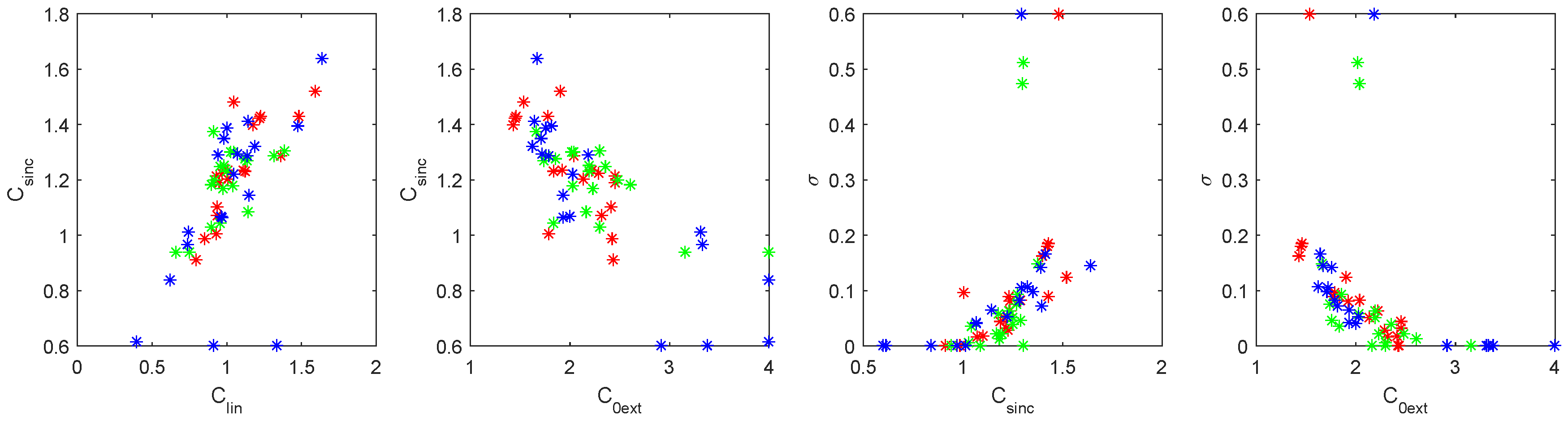
The presented models share common features, and four most significant inter-dependencies between the parameters of presented models are depicted in Figure 9. As can be seen from the panel on the left, the linear model and the simple sinc model parameters are in linear relation, as both parameters describe the steepness of the function. When comparing the model parameters with the RVoG model, it appears that all of the parameters are mainly related to the extinction parameter of the RVoG model. This indicates that in the RVoG model, the extinction parameter is perhaps more significant than the ground-to-volume ratio.

7. Discussion

All four models perform well in describing the relationship between forest height and interferometric coherence magnitude. A single-parameter linear model shows a surprisingly balanced performance throughout the different conditions and imaging geometries. However, the linear model has a clear bias in the high coherence areas. In this region, the semi-empirical sinc model, on the other hand, provides good agreement with the data. However, both the linear and sinc model fail in describing the low coherence areas when stand height is close to the height of ambiguity. The best flexibility is provided by the two-parameter RVoG model, but unfortunately, two exponential parameters make the model rather unstable. The best compromise is provided by the empirically-parametrized zero extinction model, derived from RVoG.

Our analysis of the model fitting experiments supports the idea about the similarity of the electrophysical and ecological parameters of stands (e.g., extinction, tree density) on the same image that belong to the same tree species. This is demonstrated by the fact that even a large amount of different forest stands agree with the same empirical model curve, defined by a single empirical parameter. At the same time, this empirical parameter might slightly vary from scene to scene. This implies that variation between the stands that belong to the same forest type can be much smaller than the variation between the same stands acquired on different dates. The best agreement with the models was achieved in cold imaging conditions, indicating that in cold conditions, the forest stands’ electrophysical parameters are probably most similar. This result indicates that the auxiliary information of tree species should be incorporated into routine forest height estimation whenever possible.

The work also indicates that in cold winter conditions, the assumption of similar extinction and ground reflection properties among similar forest types holds best and might be used for estimating forest height or forest extinction properties via model inversion. The results also show that when used for the purpose of forest height retrieval, the optimal height of ambiguity of the interferometric system should be around twice as large as the expected maximal forest height. It is observed, specifically for RVoG and sub-zero winter scenes, that decreasing the height of ambiguity does not increase the fit error, but rather introduces better dynamics for model inversion. This is expected to lead to better height retrieval accuracies. On the other hand, when the height of ambiguity of the interferometric system is in the order of the maximal stand height, models do not perform very well, and variations in the extinction properties introduce significant differences. Furthermore wet conditions introduce large variations, and model fitting by assuming similarity between the stands of the same forest type gives poor results.

This work also shows that both positive and negative correlation between forest height and coherence are possible and can also be described by the models. The positive correlation is observed in the areas where stand heights approached the height of ambiguity, within the so-called “tail” region of the model.

A set of models described in this work can be further used for predicting forest tree height and other relevant forest parameters, both on the stand level and the grid level.

8. Conclusions and Future Work

In this paper, space-borne interferometric X-band SAR coherence data and ALS-measured forest stand heights are used for comparing four different forest coherence models linking forest height and coherence magnitude. In addition to the random volume over ground model, three semi-empirical models are derived requiring only one fitting parameter: a simple linear model, a sinc model and a zero extinction 0ext model. Moreover, it is shown that instead of the forest height, the height relative to the height of ambiguity should be used as a parameter in the model fitting. Using such relative forest height as an argument simplifies the models and provides a common basis for the assessment of different models and approaches despite differences in the imaging geometry.

Four models are compared to each other in the proposed framework and validated against a large dataset of coherence magnitude and ALS data over hemiboreal forests in Estonia. Both positive and negative correlation between forest height and coherence are captured and can also be described by the models. The positive correlation is observed in the areas where stand heights approached the height of ambiguity, within the so-called “tail” region of the model.

In addition to the models, the variation range for empirical model parameters is also given for hemiboreal forest, paving the road towards forest stand height maps derived from InSAR coherence measurements. Overall, these models establish the basis for a simple semi-empirical modeling approach that is capable of successfully describing the dynamics of InSAR coherence observed over boreal and hemiboreal forests. Further work will concentrate on actual forest height inversion using the proposed set of models.

The future work will concentrate on the application of the proposed models for tree height retrieval and potentially forest stem volume estimation taking into account species-specific allometric approaches. Further developments will consider producing estimates on the grid level rather than the stand-wise approach, as stand information might not be available for large-scale operational applications.