Weak Environmental Controls of Tropical Forest Canopy Height in the Guiana Shield

Abstract

Canopy height is a key variable in tropical forest functioning and for regional carbon inventories. We investigate the spatial structure of the canopy height of a tropical forest, its relationship with environmental physical covariates, and the implication for tropical forest height variation mapping. Making use of high-resolution maps of LiDAR-derived Digital Canopy Model (DCM) and environmental covariates from a Digital Elevation Model (DEM) acquired over 30,000 ha of tropical forest in French Guiana, we first show that forest canopy height is spatially correlated up to 2500 m. Forest canopy height is significantly associated with environmental variables, but the degree of correlation varies strongly with pixel resolution. On the whole, bottomland forests generally have lower canopy heights than hillslope or hilltop forests. However, this global picture is very noisy at local scale likely because of the endogenous gap-phase forest dynamic processes. Forest canopy height has been predictively mapped across a pixel resolution going from 6 m to 384 m mimicking a low resolution case of 3 points·km${}^{-2}$. Results of canopy height mapping indicated that the error for spatial model with environment effects decrease from 8.7 m to 0.91 m, depending of the pixel resolution. Results suggest that, outside the calibration plots, the contribution of environment in shaping the global canopy height distribution is quite limited. This prevents accurate canopy height mapping based only on environmental information, and suggests that precise canopy height maps, for local management purposes, can only be obtained with direct LiDAR monitoring.

1. Introduction

The height of a tropical forest canopy is a key feature of the functioning and dynamics of a tropical forest ecosystem [1]. Canopy height is mainly determined by the natural regime of disturbances inducing the gap-phase forest dynamic [2], but also depends heavily on the impacts of human activity such as fire occurrence in disturbed forests [3] or logging activity in production forests [4]. In the global change context, precise knowledge of forest canopy height is also a prerequisite to accurately predict the aboveground forest biomass, a key component of the terrestrial carbon cycle [5]. At the individual tree level, forest canopy height is an important parameter to improve tree allometric equations [6]. Indeed, most allometric equations estimate this height value from a statistical inference procedure based on tree diameter at breast height, which add its own uncertainty. Therefore, alternative strategies to independently measure canopy height from the field or via remote sensing tools would greatly improve the accuracy of tree aboveground biomass estimates [7]. At the forest landscape level, carbon mapping relies very often on forest height mapping derived from remote sensing products [8].

Despite the importance of canopy height information for scientific issues related to current global changes, our knowledge about the drivers and the natural variation of tropical forest heights remain scarce. We do know the general latitudinal gradient of forest canopy heights [9] and the differences between continents, but it is often assumed that canopy heights in tropical forests are quite homogeneous within major basins (Amazonia, Africa, Southeast Asia). In the Amazonian region, for instance, the terra firma forests are often seen as having homogeneous structures and dynamics properties [10]. This may hide strong local variations that are essentially related to (i) changes in the availability of water resources and (ii) changes in soil topography associated with variations in soil fertility, soil depth, or wind exposure, all being intimately linked to the geomorphological landscape [11].

At the global scale, the canopy height of tropical forests tends to be higher in areas that are wetter and/or have low climate seasonality, so that water availability has often been viewed as a key driver [12]. Water availability is linked to two processes [13]: precipitation and water redistribution. The supply of precipitation obviously conditions the water availability for trees, but local soil properties, such as soil drainage and topographic features, modulate the local water availability for trees. The links between topographic indexes, such as the distance from the nearest channel and tree growth, are now very well established [14,15].

Recently, indexes related to landscapes and landforms features were successfully used to infer floodplain areas, drainage conditions, soil properties, and the hydrological network [11]. At a local scale, topographic variables such as slope, aspect, and curvature are often invoked to understand the drivers of forest structure [15,16], gap distribution or dynamic [17], and spatial distribution of species [18]. Despite the field evidence suggesting that topography shapes forest height variation [19], few studies so far have investigated in detail the ecological processes underlying the association between tropical forest canopy height and topographical characteristics. For instance, it could be expected that forest canopy height decreases with increasing elevation because of lower nutrient content in soil and water availability during the dry season in elevated positions on the landscape. Another important ecological driver directly related to the topography is wind speed. Wind exposure was shown to control the tropical tree growth and mortality at least in very windy island systems [20] and hurricane-prone regions [21,22]. Lobo et al. [17] successfully used the Topographic Exposure index (TOPEX) developed by [23] to predict gap formation and variation of canopy height in a continental/interior forest in Panama. In the last decade, airborne Light Detection and Ranging (LiDAR) has become a reliable remote sensing technique for estimating individual tree and stand parameters in forestry, due to its capability to generate detailed and accurate three-dimensional tree information and can be deployed from space, on the ground or in an aircraft [24]. LiDAR offers the possibility of reducing inventory costs and improving estimations of biomass at large scale [25]. For instance, LiDAR has been used to estimate structural element such as basal area, stand volume [26] and thus gives not only information about the landscape topography but also about the structure of the forest [27]. Several studies have demonstrated that LiDAR data such as Digital Canopy Model (DCM) provide an accurate information of vegetation height to estimate forest carbon [9,28], structural differentiation between primary or secondary forest and human disturbance [29,30,31]. In temperate forest, LiDAR data and Landsat ETM+ data are used in combination to analyze spatial structure and to map canopy height [32]. It was shown that an integrated modeling strategy is most suitable for estimating and mapping canopy height at locations unsampled by LiDAR. Recently in French Guiana Fayad et al. [33] used ICESat/GLAS to create a map of canopy height by using random forest regression. Their results show that it is possible and that accuracy of the prediction depend of point density of the calibration data-sets used such as space-borne LiDAR. Few studies investigates the relationship between forest structure and environmental variables and the effect of sampling strategy on the accuracy of the canopy height map prediction with airborne LiDAR in French Guiana. It is interesting to understand the mechanisms that control forest structure and provide a map of forest canopy height for forest manager at large scale. However, a common feature of data regularly sampled in space, such as the LiDAR and environmental variables used in this study, is that they typically exhibit spatial autocorrelation [34]. Most statistical tests of association require independence between observation data, a condition always being violated when autocorrelation is present within the data [35]. In this study, we take advantage of a randomization method recently developed by [36] to test the association between two spatially structured variable sets. In the present study, we use high-resolution maps of LiDAR-derived DEM and DCM to investigate the role of a large panel of potential environmental drivers on variations in forest height in tropical forests. More specifically, we address the following questions:

• What is the scale and magnitude of spatial autocorrelation of tropical forest heights?
• Are there links between environmental variables and canopy heights in tropical forests and do these links depend on the spatial resolution of the LiDAR-derived maps?
• Are environmental variables important drivers of tropical forest canopies and do they bring useful information in the perspective of predictive mapping?

2. Material and Methods

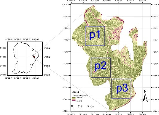
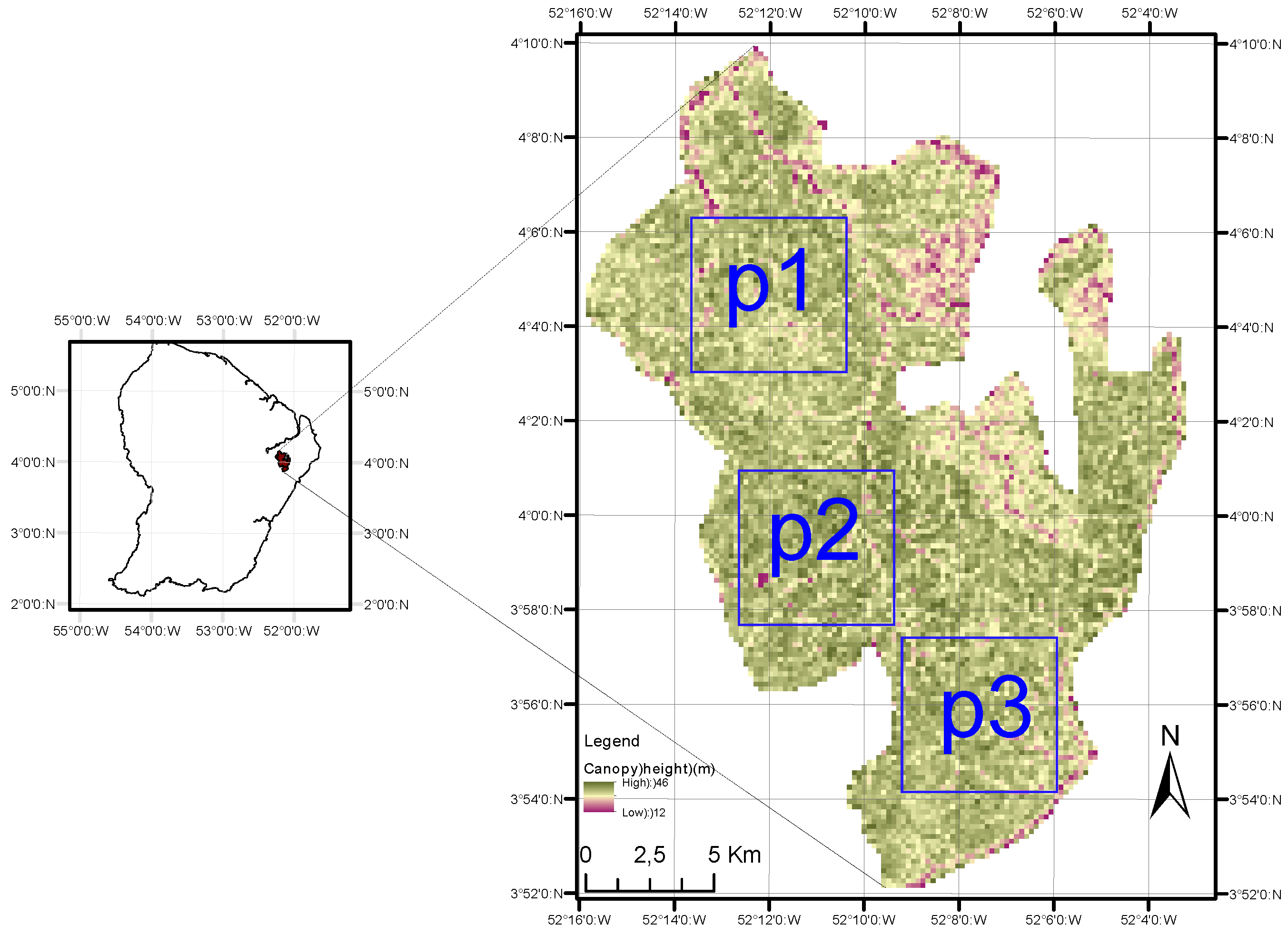
2.1. Study Site

The study site is located in the Regina forest (4${}^{\circ }$N, 52${}^{\circ }$W) (Figure 1). The most common soils in the Regina forest are ferralitic soils. The site is located on slightly contrasting plateau-type reliefs that are rarely higher than 150 m on average. The forest is typical of Guianan rainforests. The dominant families in the Regina forest include Burseraceae, Mimosoideae and Caesalpinoideae. The site receives 3806 mm of precipitation per year, with a long dry season from mid-August to mid-November, and a short dry season in March [13].

2.2. LiDAR DEM and DCM

LiDAR data were acquired in 2013 over 30,000 ha of forest by a private contractor, Altoa [37] by aircraft. The LiDAR system used for acquisition was a Laser Riegl LMS-Q560. This system was composed of a scanning laser altimeter with a rotating mirror (Riegl LMS-Q560), a GPS receiver (coupled to a second GPS receiver on the ground), and an inertial measurement unit to record the pitch, roll, and heading of the aircraft. The laser wavelength was 0.9 $\mathsf{\mu }$m (near infra-red) . The aircraft flights were conducted at 500 m above ground level with a ground speed of 180 km·h${}^{-1}$. Each flight derived two acquisitions. The LiDAR was operated with a scanning angle of 60${}^{\circ }$ and a 200 kHz pulse repetition frequency. The laser recorded the last reflected pulse with a precision better than 0.10 m with a density of 5 pulses·m${}^{-2}$. The ground routine of Terrascan software (Terrasolid Ltd., Helsinki, Finland) was used to filter raw points and identify ground echoes from which the Digital Elevation Model (DEM) was derived from a triangular interpolation network. A Digital Surface Model (DSM) was then obtained by extracting the highest echo on a 1 m grid, and a canopy height model (DCM) was finally derived by subtracting the 1 m-resolution DTM from the 1 m-resolution DSM. Because Deblauwe’s [36] algorithm requires square raster maps, we clipped three plots in the natural forest: p1, p2, and p3 (Figure 1).

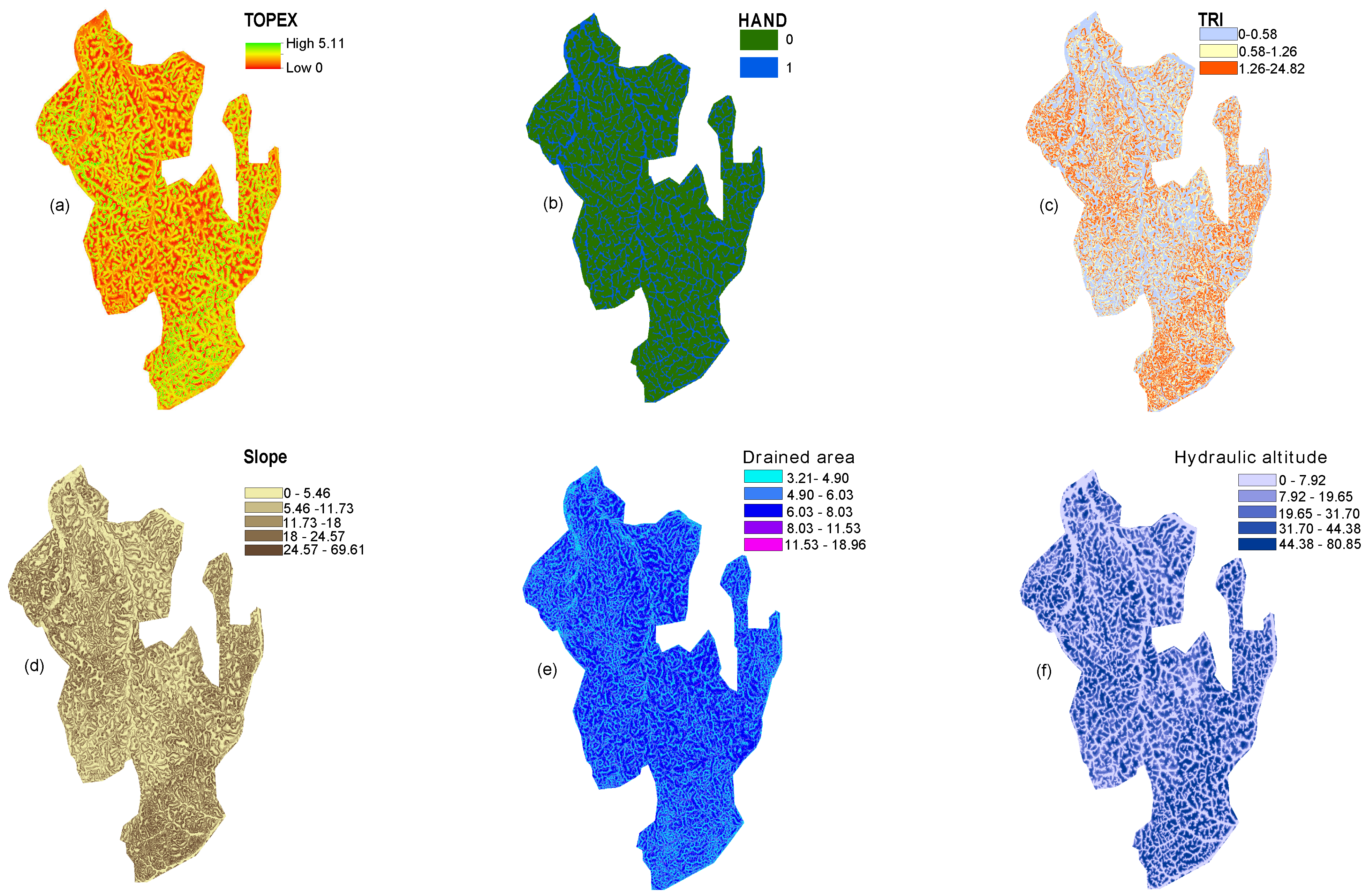
2.2.1. Environmental Variables

In order to evaluate the relationship between the DCM and the environment, we extracted several topographical and hydrological variables that we believe are important for driving canopy height variation (Figure 2) (

Table 1. The six environmental variables used in this study, with description, abbreviation, and observed range.

Environmental Variable	Abbreviation	Range	Unit
Slope	Slope	(0.1∘69.9)	${(}^{\circ })$
Terrain Ruggedness Index	TRI	(0.01–5.2)
Topographic Exposure	TOPEX	(1–4.9)
Drained Area	DA	(3.2–18.4)
Hydraulic Altitude	HA	(0–78.6)	m
Height Above the Nearest Drainage	HAND	(0–1)	m

). All variables were computed from a LiDAR Digital Elevation Model (DEM) with $25{\mathrm{m}}^2$ cells.

Hydrological variables

• The Drained Area (DA) was extracted. The DA measures the surface of the hydraulic basin that flows through a cell. A low value indicates cells located on the border between two basins, whereas the highest values indicate cells located downstream.
• The Hydraulic Altitude (HA) was computed from the 3rd order hydraulic system. The HA of a cell is its altitude above the closest stream of its hydraulic basin.
• In order to map terra firme versus floodplain forest, we used a predictive model adapted from the HAND topographic algorithm (Heigh Above the Nearest Drainage ) using a high resolution DTM. The HAND binary index has been developed to model soil water conditions in Amazonia rainforest and proved to provide good proxy of permanent water saturation in other contexts [38]. We classify pixels with HAND ≤ 2 m as floodplain and other pixels as terra firme.

Topographical variables

• We computed the slope from the DEM as the maximum rate of change in elevation from a cell to its eight neighboring cells over the distance between them.
• The Terrain Ruggedness Index (TRI) catches the difference between flat and more mountainous landscapes. The TRI was calculated using Arc-GIS 10.2 as the sum of the change in altitude between a grid cell and its eight neighbors.
• We used the Topographic Exposure index (TOPEX) to measure exposure to the wind. TOPEX is a variable that represents the degree of shelter assigned to a location. TOPEX was derived from the quantitative assessment of the horizontal inclination. The values of this index are closely correlated with the wind-shaped index. Exposure is calculated based on the height and distance of the surrounding horizon, which are combined to obtain the inflection angle. We used this angle to quantify topographic exposure. A higher inflection angle is equal to a lower exposure or more shelter [23].

2.3. Data Analysis

As input data, we extracted three large plots (p1, p2, p3, each 3782.25 ha, corresponding to a grid with 1230 × 1230 grid cells of 25 m${}^2$) in our study area. The three plots were chosen in order to cover the maximum area of LiDAR coverage. The shape of the plots is important because the Deblauwe algorithm what we use only works with square rasters (number of lines = number of columns).

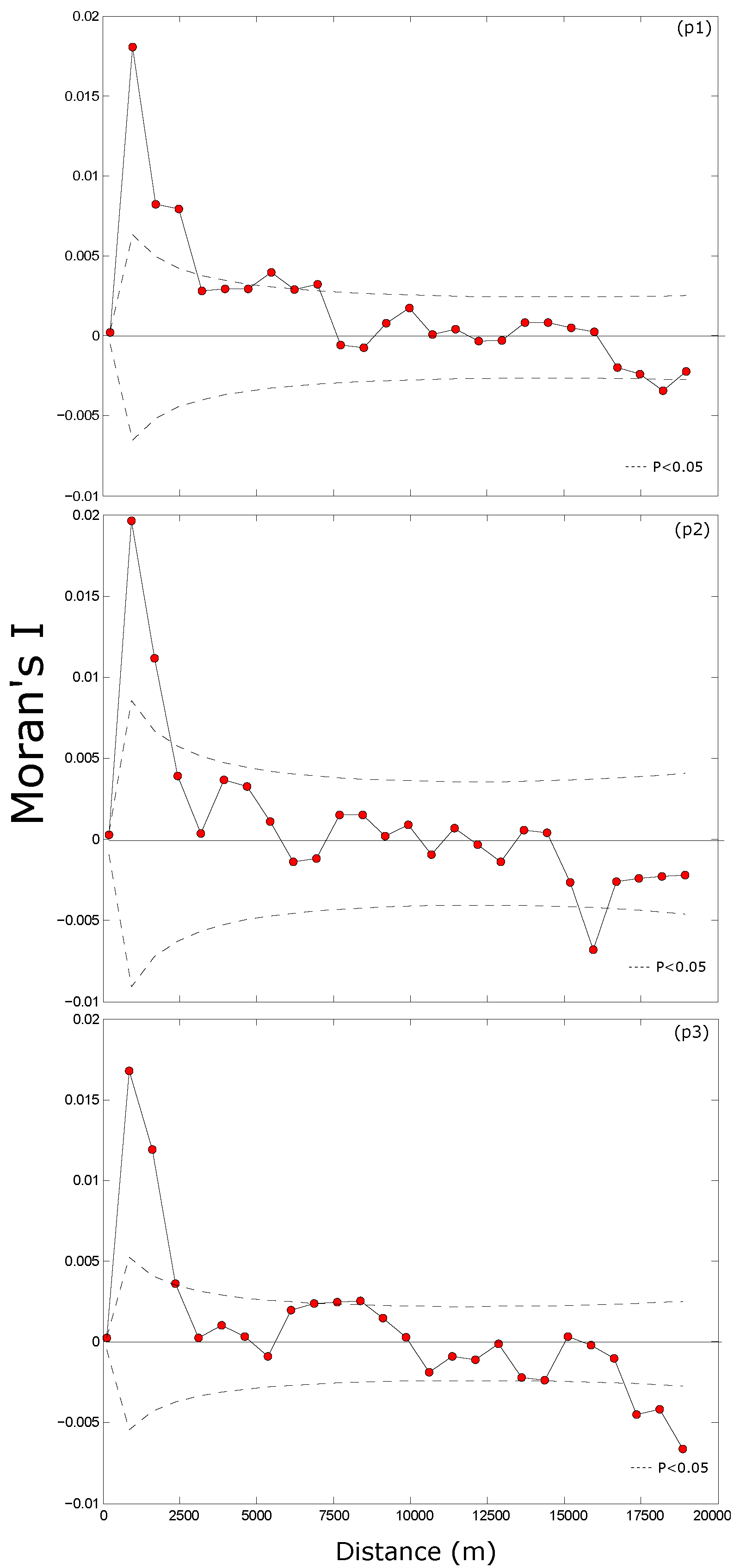
2.3.1. Spatial Autocorrelation

The scale and magnitude of spatial autocorrelation in canopy height was determined using the Moran index [39]. Moran’s Index is based on the a priori specification of neighborhood connections between observations, taking values close to 1 in case of positive spatial autocorrelation, close to −1 in case of negative spatial autocorrelation, and close to 0 when there is no spatial autocorrelation. We obtained a Moran correlogram, which represents the values of the Moran Index according to distance (cell size: 5 m) in plots p1, p2, and p3.

2.3.2. Link between Forest Canopy Height and Environmental Drivers at Different Scales

We used a wavelet-based technique developed by [36] on squared plots, to test pairwise association between the spatial structure of the digital canopy model and the environmental variables at multiple scales. The procedure can be applied to an unbiased test of any test statistic of association. We chose to test the Pearson’s product-moment correlation coefficient $r_{obs}$ between gridded data sets of canopy height and environmental data.

We calculated confidence intervals for the null hypothesis of no correlation ($H_0$: r = 0) using Monte Carlo methods. Specifically, we randomized one of the processes, in our case the DCM (canopy height data), in a way that preserves the same probability density function as the original template and also preserves the autocorrelation function. From Monte Carlo simulations, we generated 999 Dual-Tree Complex Wavelet Transform (DT-CWT) data surrogates for the DCM and environmental variable (in a quadrat subset) to determine the p-value of the null hypothesis. DT-CWT, is an improvement on classical discrete wavelet transform techniques that is immune to shift dependence, i.e., major variations in the distribution of discrete wavelet transform coefficient energy over scales and orientations caused by small integer displacements of the pattern. DT-CWT also has the advantage of a better distinction and reproduction of possible pattern directions. We then compared the correlation between the observed DCM and environmental variables with the $95\%$ confidence interval generated from these surrogates. In the case of Pearson’s product-moment correlation coefficient, which may vary between −1 and 1, the test is two-tailed, and we consider the proportion of simulations for which the correlation $r_{sim}$ falls outside the interval $[-r_{obs},r_{obs}]$ where $r_{obs}$ is the observed Pearson’s correlation coefficient. Because hydrological and topographic variables are structured at multiple scales, and in order to assess the importance of the spatial scale in shaping the link between forest canopy height and environmental drivers, we apply the test to the grids re-sampled at six different resolutions: 1024, 512, 256, 128, 64, and 32 pixels, which correspond to 6, 12, 24, 48, 96, 192, and 384 m per pixel, respectively. Conversion to larger pixel size was done by using the “aggregate” function of the Raster package, using the mean height estimate.

2.3.3. Prediction of Forest Height from Environmental Drivers

We predicted the forest canopy height using Kriging with the following Equation (1):

$$\widehat{z}\left(s_0\right)=\widehat{m}\left(s_0\right)+\widehat{e}\left(s_0\right)=\widehat{z}\left(s_0\right)+\sum _{i=1}^n{\lambda }_i\times e\left(s_i\right)$$

(1)

where $\widehat{z}\left(s_0\right)$ is the predicted value at an unsampled location $s0$, $\widehat{m}\left(s_0\right)$ is the fitted trend, $\widehat{e}\left(s_0\right)$ is the Kriging residual, ${\lambda }_i$ are the Kriging weights determined by the spatial autocorrelation structure (variogram) of the residual, and $e\left(s_i\right)$ is the residual at location $s_i$. We used the Ordinary Kriging (OK) model, allowing the interpolation of unsampled data from the semivariogram [40]. The semivariogram plots the semivariance γ as a function of the distance between samples h:

$$\gamma \left(h\right)=\frac{1}{2N\left(h\right)}\sum _{i=1}^{N\left(h\right)}{[z\left(s_i\right)-z(s_i+h)]}^2$$

(2)

where $\gamma \left(h\right)$ is the semivariance as a function of the lag distance h, $N\left(h\right)$ is the number of pairs of data separated by h, and z is the estimated canopy height at locations u$s_i$ and $(s_i+h)$. Three parameters are commonly used to model the behavior of semivariograms:

• The range is the lag distance at which the sill is reached. The range is the distance where the spatial correlation vanishes and the variogram levels off.
• The sill is the semivariance at the lag distances above which there is no spatial autocorrelation.
• The nugget is the semivariance at a lag distance of zero; it represents the spatial variability below the sampling frequency.

In this study, we postulated an exponential form to the covariance model, which takes the form:

$$\gamma \left(h\right)=c_0+c\left\{1-exp(-3\left(\frac{h}{a}\right)\right\}$$

(3)

where a is the range, h is the lag, $c_0$ is the nugget, and $c_0+c$ is the sill. For each case, the mean semi-variance was computed for 10 distance classes (i.e., limits at 250 m, 500 m, 1 km, 1.5 km, 2 km, 2.5 km, and 3 km) and compared with the null hypothesis of an absence of spatial structure simulated by 999 randomizations of canopy height. OK was then used to estimate values of $\widehat{z}$ at location $s_0$ using the following Equation (4):

$$\widehat{z}\left(s_0\right)=\sum _{i=1}^n{\lambda }_i\times z\left(s_i\right)$$

(4)

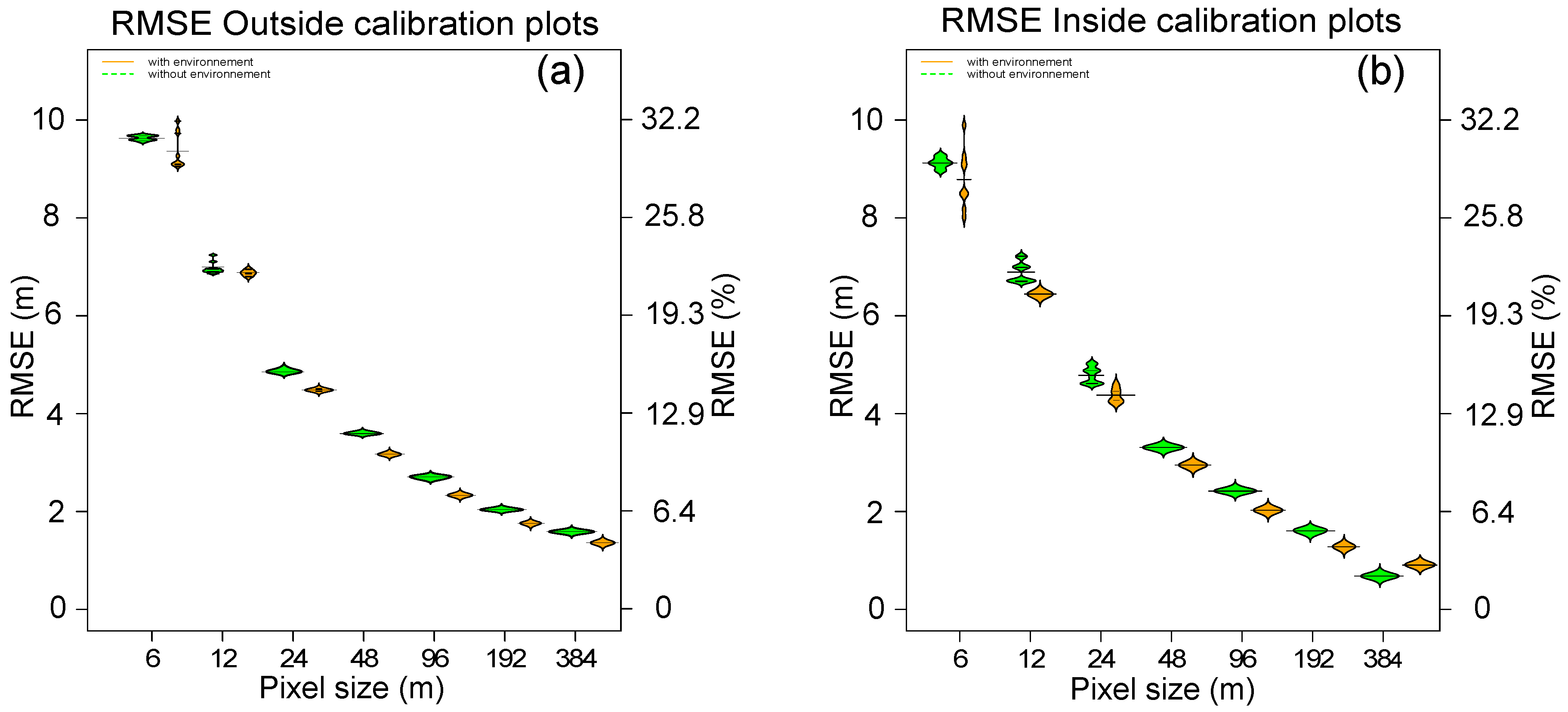
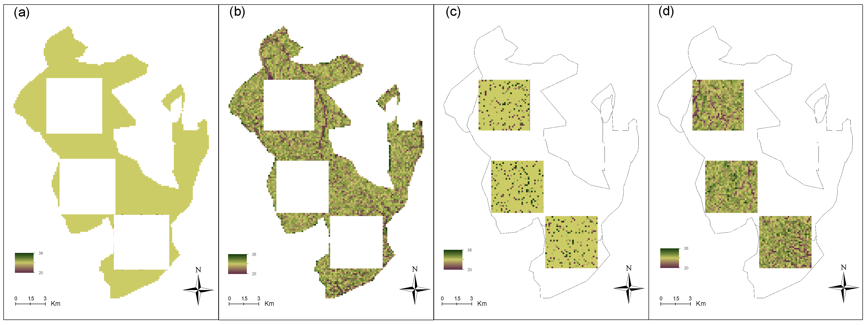
2.3.4. Strategies to build height maps

We first sampled 500 points from p1, p2, and p3, and for each pixel size (6, 12, 24, 48, 96, 192, and 384). We chose 500 points because this number corresponds to a low-resolution case (GLAS spaceborne) of about 3 points·km${}^{-2}$. Then, we made two types of predictions:

• Inside the calibration plots, where we compared the prediction with and without environmental covariates (Slope, TOPEX, TRI, HA, DA, HAND)
• Outside the calibration plots, where we compared predictions with environment-only to a null model (no calibration points, no environment)

To do so, we defined a regularly spaced grid covering the study area with pixel sizes of 6, 12, 24, 48, 96, 192, and 384 m. For each pixel size and for each type of prediction (with and without environment, inside or outside), 10 maps were computed, a new sampling of 500 points each time to generate confidence intervals. For each pixel size, the canopy height was predicted and the accuracy of the spatial prediction of canopy height ($\overline{H}$) was assessed by comparing predicted values with LiDAR values (H) from DCM using the Root Mean Square Error ($RMSE$):

$$RMSE=\sqrt{\frac{1}{N}\sum _{i=1}^N(H_i-{\overline{H}}_i{)}^2}$$

(5)

Arc-GIS 10.2 software was used to create environmental variables from DTM. MATLAB software (The MathWorks Inc., Natick, MA, USA, 2012) was used to perform environmental variable association tests. Most of the analysis was performed with the R project software [41] and more specifically, with the following packages: rgdal [42] and maptools [43].

3. Results

3.1. Spatial Variability of Canopy Height

In order to characterize the range of magnitudes of the spatial autocorrelation, Moran’s Index was used for each plot (p1, p2, p3). The three correlograms are very similar and significant at low distances ($I_{p1}=0,018;I_{p2}=0.019;I_{p3}=0.017$) (Figure 3). The main conclusion is that Moran’s Index decreases with distance and is non-significant beyond 2500 m.

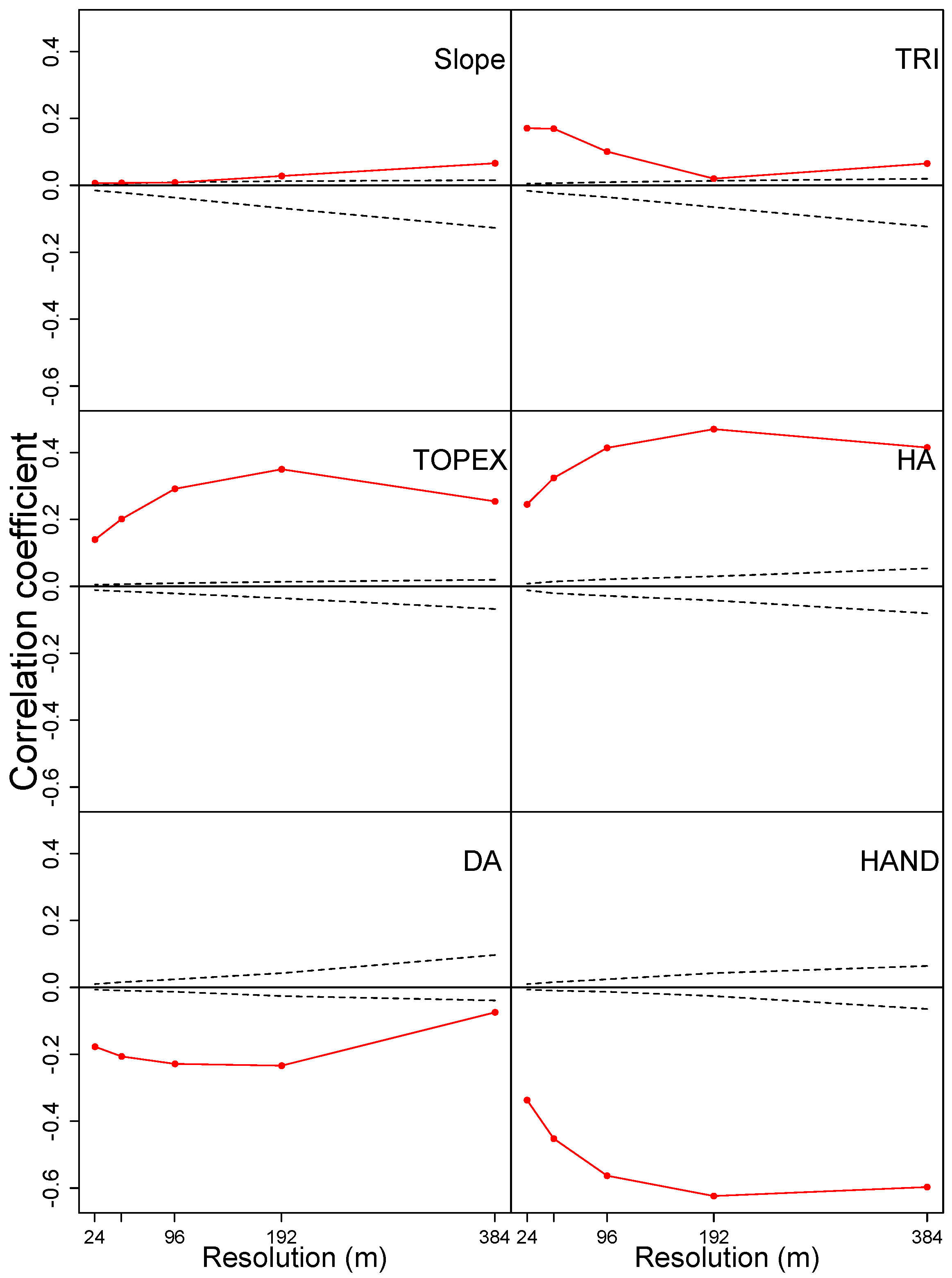
3.2. Environmental Drivers of Canopy Height

We found that the investigated environmental variables were significantly correlated with forest canopy height and that the degree of correlation varied strongly with the pixel size for all variables except the slope (Figure 4). We note a decrease in the absolute value of most coefficients of correlation when pixel sizes decrease. We observed (i) two variables negatively correlated with forest height: HAND and DA; and (ii) four variables positively correlated: TOPEX, HA, TRI, and SLOPE.

3.2.1. Effect of Hydrological Variables

We found a very strong positive correlation between HA and canopy height variation for a pixel size of (192 m × 192 m), r = 0.47, p-value < 0.001. The HAND index also showed a very high correlation with forest canopy height, with the highest for a pixel size of 3.6 ha (192 m × 192 m), r = −0.62, p-value < 0.001.

3.2.2. Effect of topographical variables

TOPEX was positively correlated with canopy height r = 0.34, p-value < 0.001; when the canopy was exposed to wind, we observed an increase in canopy height. TRI was a positive predictor of canopy height variation with a pixel size of 0.14 ha (12 m × 12 m), where we observed a maximum of coefficient correlation, r = 0.17, p-value < 0.001. Finally, we found non significant correlation between slope and canopy height with r = 0.066, p-value = 0.41.

3.3. Mapping Forest Canopy Height

3.3.1. Case 1: Inside Calibration Plots

RMSE values generally decreased from 6 m to 384 m, from RMSE${}_6$ = 8.7 m to RMSE${}_{384}$ = 0.91 m (Figure 5b), with environmental covariates and from RMSE${}_6$ = 9.12 m to RMSE${}_{384}$ = 0.68 m without. Environmental covariates slightly improved the prediction accuracy, except for a pixel size of 384 m (Figure 5b).

3.3.2. Case 2: Outside Calibration Plots

RMSE values generally decreased from 6 m to 384 m, from RMSE${}_6$ = 9.36 m to RMSE${}_{384}$ = 1.3 m with environmental covariates and from RMSE${}_6$ = 9.6 m to RMSE${}_{384}$ = 1.5 m without. Environmental covariates always, but only slightly, improved the prediction accuracy (Figure 5b).

4. Discussion

In this study, we investigated the spatial structure of canopy height variations and its relationship with the environment across spatial scales of 6 to 384 m using high-resolution maps of LiDAR-derived digital canopy height and elevation for 30,000 ha of tropical forests in French Guiana.

4.1. Spatial Auto-Correlation in Forest Canopy Height

As hypothesized, canopy height is spatially auto-correlated at a fine scale. However, we highlight a residual spatial structure even at long distance (i.e., 2500 m) that was not really expected. This suggests that canopy height variation results from complex interactions with biotic and abiotic factors at various spatial scales. Taking into account this spatial structure is thus of primary importance for predictive mapping. For instance, Fayad et al. [33] strongly improved the precision of canopy height estimates using regression Kriging (from 6.5 to 4.2 m in RMSE using the GLAS dataset, and from 5.8 to 1.8 m using an airborne LiDAR dataset).

4.1.1. Spatial Structure at Fine Scale

At fine resolution, the individual tree crown structure may be detectable and drives the auto-correlation signal [44]. In the same way, a forest gap induced by a single tree fall [45] can be observed, and structures the LiDAR signal. Gap phase dynamics play an important role in forest structure, because the formation of gaps creates openings from 10 m${}^2$ to 1000 m${}^2$, which provide ideal conditions for tree growth but also modify the forest height by creating disrupted forest canopies. At this fine spatial scale, competition for light between individual trees colonizing the forest gaps drives the changes, in time and in space, in forest canopy height. Such competition for light leads to tree crown rearrangement and to the clustering of trees growing together in the form of homogeneous patches of similar canopy height up to 60 m [46,47]. These higher biotic interactions, typical of many tropical forests, are likely to drive the spatial structure of forest height at fine scale. Our results thus suggest that observations of canopy height with high resolution give useful information on the spatial extent of forest dynamics. Another possible explanation for the spatially structured forest height at fine scale is related to the fine-scale spatial structure of the forest environment [48]. Clark et al. [2] observed that the spatial structure of abiotic factors such as soil types or topographical levels in tropical forests may modify tree growth in both diameter and height. We thus have to keep in mind that abiotic factors such as edaphic conditions may also indirectly contribute to create spatial structures of forest height at very fine scale.

4.1.2. Spatial Structure at Large Scale

The spatial auto-correlation at large scale (>100 m) could be explained by landscape-scale variation in topography. For instance, several studies observed that dendrometric (diameter and height) measurements and allometric relationships for one species could be different according to the type of soil [6], which is directly linked to the type of water drainage [11]. Indeed, in French Guiana [49], examined in detail the spatial distribution of vegetation in 19 ha of tropical forests and concluded that large soil drainage classes affect tree height. Moreover, at even larger scales, geomorphology and landform variations may contribute to modify the forest canopy height [50]. On our three plots, we observed a deep vertically draining soil and the same type of landscape [11]. We may thus suppose that the absence of spatial structure in forest canopy height at very long distances (greater than 2500 m) is partly linked to the low geological and geomormophologic variation of our study area.

4.2. Detecting Environmental Drivers with Multi-Scale Analysis

Many authors link the canopy height of mature forests to edaphic factors, and notably, to drainage conditions [50] . Our results expand on previous findings on the influence of topographic variation on tropical forest structure by identifying the major topographic variables and the scales at which relationships are strongest, and by clearly illustrating their link to hydrological processes.

4.2.1. Observations from Fine to Large Scale

Regardless of scale, the behaviors of the Pearson’s correlation coefficients are coherent, i.e., even with a change in pixel size, and the signs of all the correlation coefficients are not reversed. A second common observation is related to the increase in the absolute value of the correlation coefficient when the scale of observation increases. This result could be explained by the fact that at fine scale (<0.05 ha), we observe the height of each tree and the forest gap dynamic fingerprints, while at large scale (>1 ha), we observe forest height variation due to topographical heterogeneity. We thus highlight that the transition from fine to large scale removes the effects of local variations that are related to specific local forest history.

4.2.2. Effects of Specific Environmental Variables

All the environmental drivers used in this study were successfully related to forest canopy height variation. However, hydrology-related variables such as HA, HAND, and DA are much more significantly related to forest canopy height than SLOPE or TRI. Sabatier [51] noticed that the distribution of stand heights reflects soil conditions, while Lescure and Boulet [52] highlighted that soils with deep vertical drainage have a greater number of taller trees. Our results are in accordance with larger landscape scales. We observed an unexpected effect of slope and terrain ruggedness on forest height, unlike Ashton and Hall [12], who observed that in Borneo, the tallest forests are generally found on lower slopes and flat or undulating land. The Regina forest is characterized by a gentle hilly landscape comprised of ferralitic soils [49]. The ferralitic soils may have mechanical properties that make it possible to have a high canopy. Topographic exposure to wind showed a significant effect on forest height; however, this result was again not expected, i.e., canopy height was higher on the more exposed pixels. The Amazonian forests are rarely thought to be strongly affected by wind or hurricanes. However, pixels that are most exposed to wind are on hilltops where environmental conditions such as drainage, nutrients, and soil chemical properties are highly favorable to tree growth [11]. The effects of wind are well known on insular systems or in places where hurricanes are frequent [20]. In French Guiana, this is clearly not the case, and we believe that the positive effect of exposure is likely due to an indirect soil effect.

4.3. Mapping Tropical Forest Canopy Height

4.3.1. Mapping Canopy Height with Low-Resolution Remote Sensing Information

Using a few points (N = 500) to map the canopy height inside the calibration plots, we showed that (i) RMSE values remained quite high compared to a constant forest height null model; and that (ii) the input of additional ancillary environmental covariates only slightly improved the prediction accuracy (Figure 5). This result is quite surprising given that many recent studies have mapped canopy height at large scale from LiDAR spaceborne data. For instance, [47] estimated, from GLAS and 500 m Moderate Resolution Imaging Spectroradiometer (MODIS) data, a canopy height with an RMSE of 5.9 m. Building on [47], Simard et al. [9] drew a global canopy height map (RMSE of 6.1 m) making use of environmental ancillary data such as the annual mean precipitation, seasonal precipitation, annual mean temperature, seasonal temperature, and data from a DEM and percentage tree cover provided by MODIS. In these two recent studies, the use of GLAS allowed the mapping of canopy height at coarse resolution on the global scale. Our results show that forest height can indeed be estimated using points sampled from LiDAR waveforms (Figure 6), but when high-resolution mapping is needed (e.g., for forest management) it fails mostly because the environmental heterogeneity, at this scale, is too low to deeply shape the forest canopy height variation. Other problems that arise in comparing results from low-resolution spaceborne to high-resolution airborne LIDAR are that (i) the altimetric error of airborne LiDAR is better than that of spaceborne LiDAR; and (ii) GLAS Lidar values are strongly influenced by terrain slope. Indeed, Hilbert and Schmullius [53] showed that terrain slope plays a key role in the spaceborne LiDAR height estimate, while airborne LiDAR is only slightly influenced by terrain slope effects. This may explain the a priori low performance of our height model map when compared to spaceborne LiDAR studies.

4.3.2. Do Environment Variables Really Help to Map Forest Canopy Height?

On one hand, outside of the calibration plots (cases with absolutely no information), the environmental covariates only slightly improved the RMSE. On the other, inside the calibration plots (cases with low-resolution information), the environmental covariates barely helped to improve the forest height accuracy. This raises questions as to the usefulness of environmental data in predicting forest canopy height at the forest management scale (dozens of hectares). This also means that the prediction accuracy will significantly depend on the LiDAR sampling intensity and pixel resolution (Figure 5). Outside of the calibration plots, the effects of the spatial Kriging quickly disappear [32] and only the linear covariables (environment) effects remain. Because of this strong spatial structure, another sampling strategy, e.g., using transect lines, may be a good option [32,33]. However, when transect lines or subsamples with high sampling intensity are not available, the computing costs of the spatial model may seem prohibitive for mapping canopy heights at large scale. Finally, the contribution of environmental covariates is higher at low-resolution where the control of topography, landforms, and hydrological processes on the variability of forest canopy height is clear. At fine resolution, the height variability is more controlled by forest endogenous dynamic processes, e.g., the gap phase dynamic typical of many undisturbed tropical forests. It may be expected that the environment plays a key role in this endogenous dynamic [19], but its effect is hardly detectable when looking only at the forest canopy height.

5. Conclusions

In this study, we evaluated the spatial structure of the canopy in natural forests and we analyzed environmental factors affecting canopy height distribution in French Guiana. Our results provide evidence of the scale-dependent linkage of the topographical and hydrological variables in shaping the canopy structure of tropical forest. Furthermore we mapped forest canopy height on 30,000 ha with LiDAR data, it appears that it could be possible to map forest canopy height even if at fine scale they have high error values of prediction. On one hand, using the kriging method shows that prediction accuracy of forest canopy height strongly depends on sampling intensity. On the other, when we try to predict canopy height with environmental variables we observed that the pixel resolution play an important role in the final error of prediction. Future work should evaluate the generality of our results at a regional scale, and aim to elucidate the ecological mechanisms that underlie them. Studies should specifically investigate how canopy height is control by soil depth, geological formation, climate and, and how spatial variance in DCM scales in these Guiana Shield forests. Understanding the roles of different factors is likely to be challenging because many factors covary spatially. Study design, and especially appropriate choice of scales, is thus a critical issue. Well-designed studies of this kind have the potential to greatly improve our understanding of tropical forest structure for forest managment, and our ability to project the responses of tropical forests to anthropogenic global change.

References

1. Denslow, J.S. Tropical rainforest gaps and tree species diversity. Annu. Rev. Ecol. Syst. 1987, 18, 431–451. [Google Scholar] [CrossRef]
2. Clark, D.B.; Palmer, M.W.; Clark, D.A. Edaphic factors and the landscape-scale distributions of tropical rain forest trees. Ecology 1999, 80, 2662–2675. [Google Scholar] [CrossRef]
3. Andersen, H.E.; McGaughey, R.J.; Reutebuch, S.E. Estimating forest canopy fuel parameters using LIDAR data. Remote Sens. Environ. 2005, 94, 441–449. [Google Scholar] [CrossRef]
4. Okuda, T.; Suzuki, M.; Adachi, N.; Quah, E.S.; Hussein, N.A.; Manokaran, N. Effect of selective logging on canopy and stand structure and tree species composition in a lowland dipterocarp forest in peninsular Malaysia. For. Ecol. Manag. 2003, 175, 297–320. [Google Scholar] [CrossRef]
5. Brienen, R.; Phillips, O.; Feldpausch, T.; Gloor, E.; Baker, T.; Lloyd, J.; Lopez-Gonzalez, G.; Monteagudo-Mendoza, A.; Malhi, Y.; Lewis, S.; et al. Long-term decline of the Amazon carbon sink. Nature 2015, 519, 344–348. [Google Scholar] [CrossRef] [PubMed] [Green Version]
6. Molto, Q.; Hérault, B.; Boreux, J.J.; Daullet, M.; Rousteau, A.; Rossi, V. Predicting tree heights for biomass estimates in tropical forests—A test from French Guiana. Biogeosciences 2014, 11, 3121–3130. [Google Scholar] [CrossRef]
7. Molto, Q.; Rossi, V.; Blanc, L. Error propagation in biomass estimation in tropical forests. Methods Ecol. Evol. 2013, 4, 175–183. [Google Scholar] [CrossRef]
8. Saatchi, S.; Asefi-Najafabady, S.; Malhi, Y.; Aragão, L.E.; Anderson, L.O.; Myneni, R.B.; Nemani, R. Persistent effects of a severe drought on Amazonian forest canopy. Proc. Natl. Acad. Sci. USA 2013, 110, 565–570. [Google Scholar] [CrossRef] [PubMed]
9. Simard, M.; Pinto, N.; Fisher, J.B.; Baccini, A. Mapping forest canopy height globally with spaceborne lidar. J. Geophys. Res. Biogeosci. 2011, 116, G04021. [Google Scholar] [CrossRef]
10. Baraloto, C.; Rabaud, S.; Molto, Q.; Blanc, L.; Fortunel, C.; Herault, B.; Davila, N.; Mesones, I.; Rios, M.; Valderrama, E.; et al. Disentangling stand and environmental correlates of aboveground biomass in Amazonian forests. Glob. Chang. Biol. 2011, 17, 2677–2688. [Google Scholar] [CrossRef]
11. Guitet, S.; Cornu, J.F.; Brunaux, O.; Betbeder, J.; Carozza, J.M.; Richard-Hansen, C. Landform and landscape mapping, French Guiana (South America). J. Maps 2013, 9, 325–335. [Google Scholar] [CrossRef]
12. Ashton, P.S.; Hall, P. Comparisons of structure among mixed dipterocarp forests of north-western Borneo. J. Ecol. 1992, 80, 459–481. [Google Scholar] [CrossRef]
13. Wagner, F.; Hérault, B.; Stahl, C.; Bonal, D.; Rossi, V. Modeling water availability for trees in tropical forests. Agric. For. Meteorol. 2011, 151, 1202–1213. [Google Scholar] [CrossRef]
14. Wagner, F.; Rossi, V.; Stahl, C.; Bonal, D.; Herault, B. Water availability is the main climate driver of neotropical tree growth. PLoS ONE 2012, 7, e34074. [Google Scholar] [CrossRef] [PubMed] [Green Version]
15. Detto, M.; Muller-Landau, H.C.; Mascaro, J.; Asner, G.P. Hydrological networks and associated topographic variation as templates for the spatial organization of tropical forest vegetation. PLoS ONE 2013, 8, e76296. [Google Scholar] [CrossRef] [PubMed]
16. Clark, D.B.; Clark, D.A. Landscape-scale variation in forest structure and biomass in a tropical rain forest. For. Ecol. Manag. 2000, 137, 185–198. [Google Scholar] [CrossRef]
17. Lobo, E.; Dalling, J. Effects of topography, soil type and forest age on the frequency and size distribution of canopy gap disturbances in a tropical forest. Biogeosciences 2013, 10, 6769–6781. [Google Scholar] [CrossRef]
18. Lan, G.; Hu, Y.; Cao, M.; Zhu, H. Topography related spatial distribution of dominant tree species in a tropical seasonal rain forest in China. For. Ecol. Manag. 2011, 262, 1507–1513. [Google Scholar] [CrossRef]
19. Ferry, B.; Morneau, F.; Bontemps, J.D.; Blanc, L.; Freycon, V. Higher treefall rates on slopes and waterlogged soils result in lower stand biomass and productivity in a tropical rain forest. J. Ecol. 2010, 98, 106–116. [Google Scholar] [CrossRef]
20. Thomas, S.C.; Martin, A.R.; Mycroft, E.E. Tropical trees in a wind-exposed island ecosystem: Height-diameter allometry and size at onset of maturity. J. Ecol. 2015, 103, 594–605. [Google Scholar] [CrossRef]
21. Gleason, S.M.; Williams, L.J.; Read, J.; Metcalfe, D.J.; Baker, P.J. Cyclone effects on the structure and production of a tropical upland rainforest: Implications for life-history tradeoffs. Ecosystems 2008, 11, 1277–1290. [Google Scholar] [CrossRef]
22. Chambers, J.Q.; Asner, G.P.; Morton, D.C.; Anderson, L.O.; Saatchi, S.S.; Espírito-Santo, F.D.; Palace, M.; Souza, C. Regional ecosystem structure and function: Ecological insights from remote sensing of tropical forests. Trends Ecol. Evol. 2007, 22, 414–423. [Google Scholar] [CrossRef] [PubMed]
23. Ruel, J.; Pin, D.; Spacek, L.; Cooper, K.; Benoit, R. The estimation of wind exposure for windthrow hazard rating: Comparison between Strongblow, MC2, Topex and a wind tunnel study. Forestry 1997, 70, 253–266. [Google Scholar] [CrossRef]
24. Palace, M.; Sullivan, F.B.; Ducey, M.; Herrick, C. Estimating tropical forest structure using a terrestrial lidar. PLoS ONE 2016, 11, e0154115. [Google Scholar] [CrossRef] [PubMed]
25. Asner, G.P.; Mascaro, J.; Muller-Landau, H.C.; Vieilledent, G.; Vaudry, R.; Rasamoelina, M.; Hall, J.S.; van Breugel, M. A universal airborne LiDAR approach for tropical forest carbon mapping. Oecologia 2012, 168, 1147–1160. [Google Scholar] [CrossRef] [PubMed]
26. Lefsky, M.A.; Cohen, W.; Acker, S.; Parker, G.G.; Spies, T.; Harding, D. Lidar remote sensing of the canopy structure and biophysical properties of Douglas-fir western hemlock forests. Remote Sens. Environ. 1999, 70, 339–361. [Google Scholar] [CrossRef]
27. Alonzo, M.; McFadden, J.P.; Nowak, D.J.; Roberts, D.A. Mapping urban forest structure and function using hyperspectral imagery and lidar data. Urban For. Urban Green. 2016, 17, 135–147. [Google Scholar] [CrossRef]
28. Popescu, S.C. Estimating biomass of individual pine trees using airborne lidar. Biomass Bioenergy 2007, 31, 646–655. [Google Scholar] [CrossRef]
29. Drake, J.B.; Dubayah, R.O.; Clark, D.B.; Knox, R.G.; Blair, J.B.; Hofton, M.A.; Chazdon, R.L.; Weishampel, J.F.; Prince, S. Estimation of tropical forest structural characteristics using large-footprint lidar. Remote Sens. Environ. 2002, 79, 305–319. [Google Scholar] [CrossRef]
30. Drake, J.B.; Dubayah, R.O.; Knox, R.G.; Clark, D.B.; Blair, J.B. Sensitivity of large-footprint lidar to canopy structure and biomass in a neotropical rainforest. Remote Sens. Environ. 2002, 81, 378–392. [Google Scholar] [CrossRef]
31. Gibbs, H.K.; Brown, S.; Niles, J.O.; Foley, J.A. Monitoring and estimating tropical forest carbon stocks: Making REDD a reality. Environ. Res. Lett. 2007, 2, 045023. [Google Scholar] [CrossRef]
32. Hudak, A.T.; Lefsky, M.A.; Cohen, W.B.; Berterretche, M. Integration of lidar and Landsat ETM+ data for estimating and mapping forest canopy height. Remote Sens. Environ. 2002, 82, 397–416. [Google Scholar] [CrossRef]
33. Fayad, I.; Baghdadi, N.; Bailly, J.; Barbier, N.; Gond, V.; Hérault, B.; El Hajj, M.; Lochard, J.; Perrin, J. Regional scale rain-forest height mapping using regression-kriging of spaceborne and airborne LiDAR data: Application on French Guiana. In Proceedings of the 2015 IEEE International Geoscience and Remote Sensing Symposium (IGARSS), Milan, Italy, 26–31 July 2015; pp. 4109–4112.
34. Congalton, R.G. A review of assessing the accuracy of classifications of remotely sensed data. Remote Sens. Environ. 1991, 37, 35–46. [Google Scholar] [CrossRef]
35. Cerioli, A. Testing mutual independence between two discrete-valued spatial processes: A correction to pearson chi-squared. Biometrics 2002, 58, 888–897. [Google Scholar] [CrossRef] [PubMed]
36. Deblauwe, V.; Kennel, P.; Couteron, P. Testing pairwise association between spatially autocorrelated variables: A new approach using surrogate lattice data. PLoS ONE 2012, 7, e48766. [Google Scholar] [CrossRef] [PubMed]
37. Altoa 2016 Website. Altoa. Maitrisez Votre Espace. Available online: http://www.altoa.org/fr/lidar.html (accessed on 10 January 2016).
38. Nobre, A.; Cuartas, L.; Hodnett, M.; Rennó, C.; Rodrigues, G.; Silveira, A.; Waterloo, M.; Saleska, S. Height above the nearest drainage—A hydrologically relevant new terrain model. J. Hydrol. 2011, 404, 13–29. [Google Scholar] [CrossRef]
39. Fortin, M.J.; Drapeau, P.; Legendre, P. Spatial autocorrelation and sampling design in plant ecology. Vegetatio 1989, 83, 209–222. [Google Scholar] [CrossRef]
40. Tsui, O.W.; Coops, N.C.; Wulder, M.A.; Marshall, P.L. Integrating airborne LiDAR and space-borne radar via multivariate kriging to estimate above-ground biomass. Remote Sens. Environ. 2013, 139, 340–352. [Google Scholar] [CrossRef]
41. R Project Software 2015. Available online: http://www.r-project.org/ (accessed on 20 December 2015).
42. Bivand, R.; Keitt, T.; Rowlingson, B. Rgdal: Bindings for the Geospatial Data Abstraction Library. R Package Version 0.8-10. Available online: https://cran.r-project.org/web/packages/rgdal/index.html (accessed on 20 December 2015).
43. Bivand, R.; Lewin-Koh, N. Maptools: Tools for Reading and Handling Spatial Objects. R Package Version 0.8-27. Available online: http://cran. r-project. org/web/packages/maptools/maptools (accessed on 20 December 2015).
44. Vincent, G.; Sabatier, D.; Blanc, L.; Chave, J.; Weissenbacher, E.; Pélissier, R.; Fonty, E.; Molino, J.F.; Couteron, P. Accuracy of small footprint airborne LiDAR in its predictions of tropical moist forest stand structure. Remote Sens. Environ. 2012, 125, 23–33. [Google Scholar] [CrossRef]
45. Asner, G.P.; Kellner, J.R.; Kennedy-Bowdoin, T.; Knapp, D.E.; Anderson, C.; Martin, R.E. Forest canopy gap distributions in the southern Peruvian Amazon. PLoS ONE 2013, 8, e60875. [Google Scholar] [CrossRef] [PubMed]
46. Bruijnzeel, L.A.; Scatena, F.N.; Hamilton, L.S. Tropical Montane Cloud Forests: Science for Conservation and Management; Cambridge University Press: Cambridge, UK, 2011. [Google Scholar]
47. Lefsky, M.A. A global forest canopy height map from the moderate resolution imaging spectroradiometer and the geoscience laser altimeter system. Geophys. Res. Lett. 2010, 37, 15. [Google Scholar] [CrossRef]
48. Harms, K.E.; Condit, R.; Hubbell, S.P.; Foster, R.B. Habitat associations of trees and shrubs in a 50-ha neotropical forest plot. J. Ecol. 2001, 89, 947–959. [Google Scholar] [CrossRef]
49. Sabatier, D.; Grimaldi, M.; Prévost, M.F.; Guillaume, J.; Godron, M.; Dosso, M.; Curmi, P. The influence of soil cover organization on the floristic and structural heterogeneity of a Guianan rain forest. Plant Ecol. 1997, 131, 81–108. [Google Scholar] [CrossRef]
50. Paget, D. Etude de la Diversite Spatiale des Ecosystemes Forestiers Guyanais: Reflexion Methodologique et Application. Ph.D. Thesis, Ecole Nationale de Génie Rural des Eaux et Forêts (ENGREF), Nancy, France, 1999. [Google Scholar]
51. Sabatier, D. Diversité des arbres et du peuplement forestier en Guyane. In Gestion de l’écosysteme Forestier et Aménagement de L’espace Régional; Actes du II éme Congrés Régional de L’Evironnement: Sapanguy, Cayenne, 1990; pp. 41–47. [Google Scholar]
52. Lescure, J.P.; Boulet, R. Relationships between soil and vegetation in a tropical rain forest in French Guiana. Biotropica 1985, 17, 155–164. [Google Scholar] [CrossRef]
53. Hilbert, C.; Schmullius, C. Influence of surface topography on ICESat/GLAS forest height estimation and waveform shape. Remote Sens. 2012, 4, 2210–2235. [Google Scholar] [CrossRef]
Figure 1. Map of study site location in the Regina forest, a lowland tropical rainforest in French Guiana (192 m × 192 m). Three 3782.25 ha plots (p1, p2, p3) are used to test the environmental effects in shaping forest canopy height. The remaining areas are used to test the predictive power of the environment-only models. Green colors represent taller canopy and red colors represent shorter canopy.
Remotesensing 08 00747 g001
Figure 2. Spatial distribution of the six environmental variables used to (i) test association and (ii) map canopy height in Regina forest: (a) TOPEX; (b) HAND; (c) TRI; (d) Slope; (e) Da; and (f) Hydraulic altitude.
Remotesensing 08 00747 g002
Figure 3. Moran’s correlograms of canopy height for plots p1, p2, and p3 in the Regina forest, French Guiana. Moran’s correlograms indicate a significant effect (p-value < 0.05) of spatial autocorrelation up to 2500 m.
Remotesensing 08 00747 g003
Figure 4. Correlation coefficients between smoothed DCM and smoothed topographic variables (defined in Table 1), as a function of the smoothing scale. Dotted lines represent the 95% confidence intervals of Pearson’s test computed from 999 simulations.
Remotesensing 08 00747 g004
Figure 5. Violin plots showing the density of the root mean square (RMSE) for 10 height prediction maps for each pixel size. Green violin plot represents RMSE without covariables, and orange violin plot represents RMSE with covariables. (a) RMSE outside plots; (b) RMSE inside plots p1, p2, p3.
Remotesensing 08 00747 g005
Figure 6. (a) DCM map derived from Kriging method outside plots without environment; the canopy height is equal to the average predicted values; (b) DCM map derived from Kriging method outside plots with environment; (c) DCM predicted with Kriging method inside plots without environment; (d) DCM predicted with Kriging method inside plots with environment
Remotesensing 08 00747 g006