1. Introduction
Remote sensing methods are often used in landscape archaeology for the acquisition of raw data. However, despite an abundance of techniques that use propagated signals to observe the Earth’s surface from above, archaeological remote sensing still relies mainly on passive air- and spaceborne imaging in the optical spectrum or the active sounding technique known as Airborne Laser Scanning (ALS) for data acquisition. Furthermore, selection of the appropriate technique is often linked to the nature of the (often hidden) archaeological remains that are expected to be discovered.
Archaeological remains can be revealed in a number of ways, but so-called vegetation marks are among the most abundant indicators of sub- or near-surface archaeological activity. Moreover, they often form the main focus of both aerial observers and image interpreters due to their potential to disclose very detailed morphological information about hidden features and structures (certainly in cereals such as wheat and barley). Sub-surface archaeological remains such as trenches or pits will often be filled with organic material and/or new soil, which often has greater moisture retention and is more nutrient-dense than the surrounding matrix. In periods of drought, these fillings might have a favourable effect on the vegetation growing on top, allowing the plants to grow profusely and for an extended period of time. The adjacent plants will be shorter, thinner, and ripen quicker, leading to differences in colour that can be seen from above as positive vegetation marks. In unfavourable situations (e.g., plants growing over buried floors or stone walls), weaker and shorter plants might occur, resulting in negative vegetation marks. Speaking in more technical terms, such adverse situations put a certain stress on the vegetation, blocking the growth, development, or metabolism of the plant. It is the senescence or stress-related decay of chlorophyll—a green pigment that can be found in all green plants and largely absorbs incident visible wavelengths in the visible blue waveband (centred around 450 nm) and visible red (around 670 nm) spectral region [
1,
2]—that induces an increased visible reflectance in the visible green to red wavebands [
3,
4]. Consequently, the plant’s dominant green colour disappears in favour of a yellow discoloration, a phenomenon called chlorosis [
5,
6,
7]. By recording the reflected portion of the visible radiation, aerial optical imaging thus allows the remote assessment of vegetation status. This can subsequently be given an archaeological interpretation [
8], although the exact physical vegetation properties still depend on the type and amount of environmental stress as well as the plant species, agricultural practices, and the chemical, physical, and biological properties of the soil (see [
9] for more details).
Apart from the differences in colour, the height of the plants could also theoretically serve as a proxy to detect changes in the soil caused by past anthropogenic activity, because the differences in the structure and composition of the soil allow plants to grow vigorously for a longer period of time. Since these local height variances in the uppermost vegetation surfaces (often referred to as the canopy) can reveal themselves as shadow marks when thrown into relief by low slanting sunlight, archaeologists have always relied upon these indirect markers of canopy height differences rather than assessing their true physical difference.
As a matter of fact, vegetation canopies that do no exhibit any archaeologically useful discoloration have generally been considered an annoyance in archaeological prospection. Prior to the advent of ALS in archaeological prospection, vegetation canopies visible in remote sensing data frequently remained an impenetrable cover, masking underlying and sometimes archaeologically significant features (e.g., barrows and hillforts covered by forest). Given its capability to digitise (overgrown) surfaces with high accuracy, ALS is able to document and visualise the geometry of very small topographic undulations such as earthworks or other (even submerged) features of archaeological interest [
10,
11,
12,
13]. Therefore, it should not come as a surprise that the introduction of ALS into landscape archaeology was mainly hailed for its ability to record sub-canopy features. Using this technology, vegetation could be digitally removed to expose the underlying terrain while also allowing for the modelling of solid standing structures. Such local topographic variations are generally visualised with a selection of 2.5D visualisation techniques, often developed by cartographers [
14,
15] or scholars working in the field of (archaeological) remote sensing [
16,
17,
18,
19,
20,
21,
22,
23].
Various non-archaeological authors, however, realised the potential of ALS data for the identification of geometrical changes in plant properties. They deliberately started to use the first rather than the last return of each laser pulse to create a dense three-dimensional point cloud of the vegetation canopy rather than the bare earth. Such a canopy model—which is sometimes denoted a Crop Surface Model (CSM) when dealing with crops [
24]—has since been commonly applied in forestry [
25,
26] and agriculture [
27,
28,
29]. The rare investigations that rely on a vegetation canopy model for archaeological vegetation mark identification [
30] indicate that, to this very day, archaeologists have still not truly realised the archaeological prospection potential of digitally encoded plant height differences.
Until a few years ago, such dense point clouds would almost exclusively be acquired using laser scanning (both airborne and terrestrial) approaches. Owing to the recent popularity of (semi-) automated image orientation techniques such as Structure from Motion (SfM) complemented by dense image-matching algorithms embedded in Multi-View Stereo (MVS) approaches, in recent years passively generated image-based point clouds have become nearly as common as their actively generated counterparts. It is easy to observe this trend in the field of airborne mapping and Digital Elevation Model (DEM) generation. Whether the end product is a Digital Surface Model (DSM) or bare-earth Digital Terrain Model (DTM), image-based dense point cloud generation as a means to digitise specific elevation surfaces can now be considered a very suitable alternative to active laser scanning approaches [
31,
32,
33,
34,
35,
36,
37]. Additionally, SfM-MVS-based georeferencing and (ortho)rectification pipelines can now deal with hundreds, if not thousands, of images at once while also properly dealing with the tilt- and topographically-induced deformations of the photographs, both of which were previously impossible using standard archaeologically-dedicated tools such as AERIAL [
38] and Airphoto [
39]. As the majority of remotely sensed archaeological data still consists of aerial photographs collected during observer-biased reconnaissance flights [
40], it is not surprising that the archaeological potential of these so-called Image-Based Modelling (IBM) approaches has been extensively explored from a number of perspectives during the past five years [
41,
42,
43,
44,
45,
46,
47,
48].
Despite these advances in aerial image processing, it seems that nobody has really explored the new possibilities that these IBM workflows could offer for vegetation mark identification (a situation that is, not surprisingly, very similar to the lack of research on the archaeological use of ALS-based vegetation height data). As was mentioned earlier, aerial image interpretation has always focused on the obvious spectral dimensions of an aerial photograph collection (i.e., the three broad spectral bands of a standard colour image). There is, however, also an inherent geometrical dimension stored in the images that can be extracted via dense image-matching techniques. Therefore, the key focus of this paper is extracting both the spectral (i.e., colour) and geometrical (i.e., absolute and relative heights) components of a crop canopy from archived analogue aerial photographs and using both parameters as proxies for archaeological prospection. Subsequently, visualisation techniques from the ALS community can help to bring out useful geometrical features that are encoded in this newly derived height dataset. Using archival imagery from an Italian case study, it will be demonstrated that a combination of the spectral and geometrical dimensions of a crop canopy can even overcome hurdles that are typical for each information set on its own.
The remainder of this paper will first introduce the case study and the research project it is part of. Next, the fundamental steps that are needed to model and visualise the canopy surface will be detailed. Along the way, the article will illustrate the unique capabilities that combining both the spectral and geometrical vegetation characteristics can provide to archaeological interpretation. Finally, we will discuss some of the current limitations and planned improvements for this workflow before this article concludes.
3. Data Processing Methods
3.1. Image-Based Modelling
To date, there are several SfM-MVS-based packages that can be employed to obtain a (semi-) automated processing pipeline for image-based three-dimensional (3D) visualisation. For this paper, all 3D models and orthophotographs were computed using PhotoScan Professional Edition (version 1.2.4), an IBM package from Agisoft LLC [
59,
60]. As can be seen in
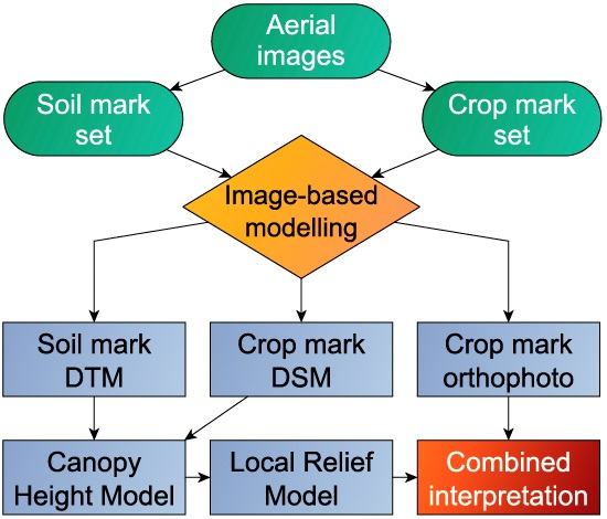
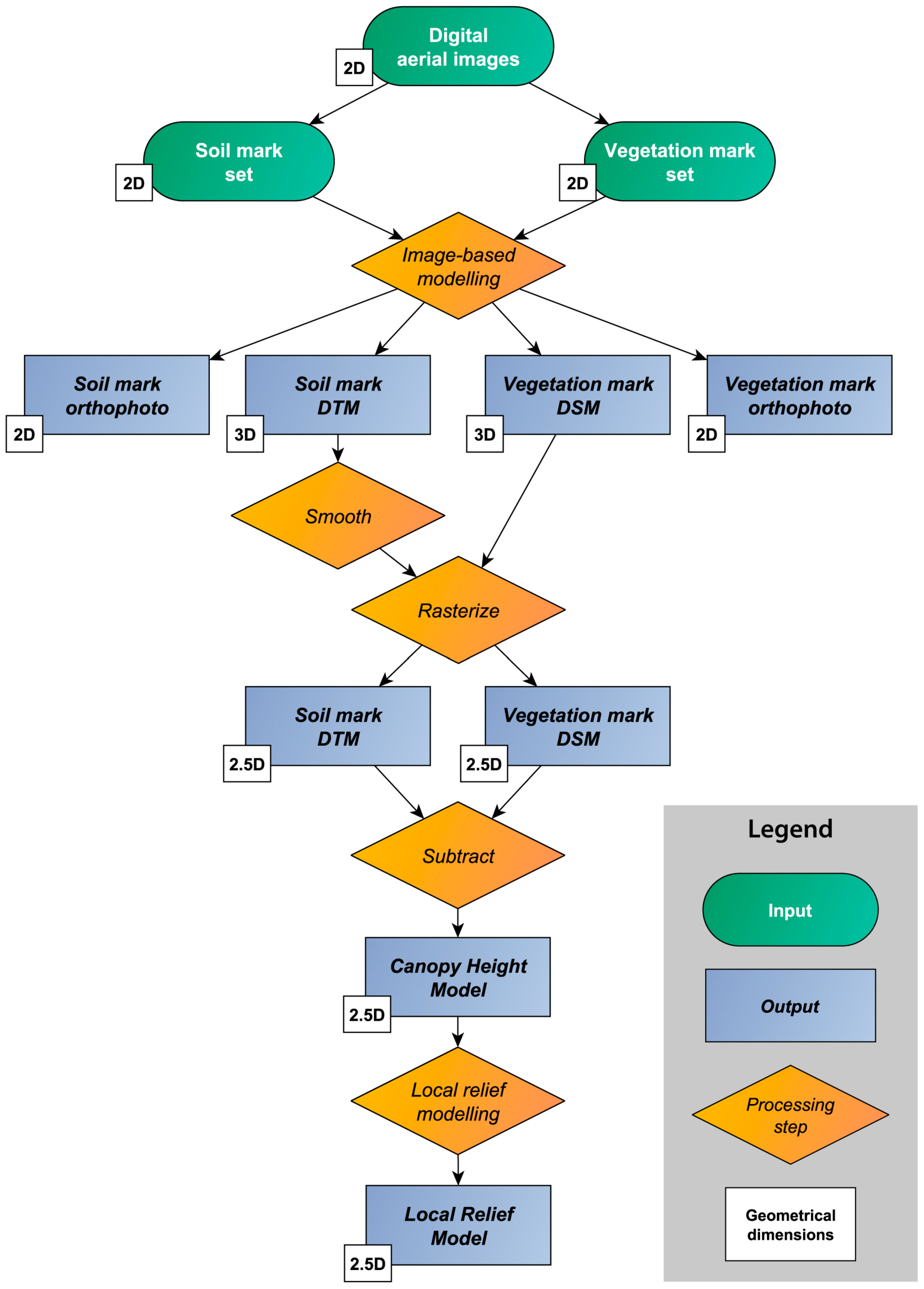
Figure 1, the IBM of both soil and vegetation mark datasets yielded an elevation model and accompanying orthophotograph. Although both photo collections were characterised by a very high overlap (70% to 100% between successive images), these steps were, however, not as straightforward as initially anticipated and several problems had to be solved before decent results could be obtained.
For the Montarice case study, three key issues could be defined: site coverage, photograph geometry, and ground control. First, the Montarice hilltop was captured once with and once without vegetation, which renders the same scene completely differently. Since this can lead to the extraction of wrong tie points on the one hand and ambiguous dense image matching results on the other hand, the only solution is to process both datasets separately. The second problem is related to the geometry of the aerial photographs. Being non-photogrammetrically scanned diapositives, several (potentially highly non-uniform) geometrical deformations come together in every image. First, every photograph suffers from distortions induced by the camera optics. These are, however, complemented by possible film deformations—resulting from film shrinkage and/or expansion due to their storage in a non-optimised environment—as well as serious geometric errors that can be introduced at the scanning stage [
61]. Moreover, the focal length of the images is unknown, which means that the SfM step does not have a suitable initial value to start from. Both factors can prevent many SfM algorithms from properly estimating the exterior camera parameters or accurately modelling the interior parameters.
In order to mitigate the issue of geometric distortion, several highly accurate Ground-Control Points (GCPs) have to be used as constraints in the SfM bundle adjustment. Although 22 GCPs were measured by differential GNSS (Global Navigation Satellite System) during the summer of 2015, almost all were located at the foot of electricity pylons. This is due to the fact that almost 13 years have passed since the acquisition of the images, making it very difficult to find targets that were distinguishable and still present in the current landscape. Additionally, a number of better potential targets were inaccessible because they were located on private property. Given the abundance of electricity pylons on Montarice, their feet were the most appropriate objects to feature as GCP. However, as the pylon feet are round, it is very difficult to determine exactly the part of the foot where the GCP has been measured. Furthermore, that part might also be invisible in the photographs from certain observation angles (
Figure 2A). Computing the pylon’s exact centre is also not an option, since it is impossible to indicate that on an image. Although the individual 3D positional accuracies of all GCPs are known to be in the two to four centimetre range, due to these factors the accuracy by which they can be indicated remains to a certain extent unknown. Moreover, many of these pylons are partly obscured by bushes or shielded by tree crowns, meaning that the ground surface (and thus the pylon’s foot) remain invisible (
Figure 2B,C). As a result, some of the GCPs could only be positioned very coarsely, while others could not be indicated at all.
Using accurately positioned GCPs as constraints in the bundle adjustment of the SfM algorithm is very important to avoid instability of the bundle solution and correct for errors in the recovered camera orientations. However, due to all of the abovementioned issues, simply incorporating the indicated GCPs in the SfM step risks seriously overestimating the camera’s interior and exterior parameters. In turn, this could lead to a 3D model that might be over-fitted and heavily geometrically distorted.
In order to address this issue, a complex and iterative IBM procedure was followed for every image collection. The soil mark dataset was processed first due to its larger coverage and the fact that the GCPs were easier to identify. Initially, 18 GCPs were indicated and the SfM step was run a number of times, gradually increasing GCP accuracy settings (i.e., 15 cm, 10 cm, 8 cm, 5 cm, 2 cm, and 5 mm). Since approximately the same subset of GCPs showed a high Root-Mean Square Error (RMSE) across all SfM solutions, a subset of three erroneous GCPs was removed and the exact same procedure was repeated. With an overall RMSE in the order of 10 cm to 15 cm, the subsequent SfM solutions were much more accurate than the initial ones, which featured overall RMSEs in the order of 20 cm to 50 cm. After cleaning the sparse point clouds of the more accurate SfM solutions by removing the tie points with the highest Reprojection Error (RE), the bundle adjustment was executed once more for every SfM solution to further optimise the camera’s interior and exterior orientation.
Given the complexity of the geometrical deformations, the amount of optimised interior orientation parameters was also varied. In the end, the numerous possible SfM solutions—all based on the same image set—were tested both quantitatively (in terms of overall and maximum RE as well as image-specific mean RE) and qualitatively (in terms of surface artefacts that were visible after densely matching the SfM solution and obvious incorrectly positioned cameras). From this analysis, it became clear that low RMSEs do not necessarily mean that the surface will be accurately constructed after dense matching. Using a GCP accuracy of 1 cm or lower leads to surface artefacts due to model overfitting of the camera orientation parameters. In the end, applying a GCP accuracy of 5 cm while solving for three radial (
k1,
k2,
k3) and two decentring lens distortion parameters (
p1,
p2) yielded the most satisfying result, with an overall RMSE of 13.7 cm (see
Table 1).
Afterwards, the same approach was followed for the vegetation dataset. In addition to a qualitative and quantitative assessment of all the vegetation-based IBM results, the resulting surfaces were also compared with the previously computed 3D soil surface. This revealed a noticeable tilt of all the vegetation surface versions with respect to the soil surface. Since the cause of this tilt could be attributed to the absence of ground control on the northern side of the Montarice flank, this issue was solved by introducing an additional GCP whose coordinates were derived from the soil mark dataset. In the end, the final solution was optimised for four radial (
k1,
k2,
k3,
k4) and four decentring lens distortion parameters (
p1,
p2,
p3,
p4) as well as two parameters (
b1,
b2) that model the affinity in the image plane (consisting of aspect ratio and skew). The GCP accuracy was again set to 5 cm. Apart from approximately identical RMSEs for the soil and vegetation datasets (see
Table 1), both 3D surfaces also coincided in non-vegetated regions such as roads and houses.
As a final step in the IBM process, an orthophotograph was computed for every dataset. Although the initial orthophotographs provided a geometrically accurate record of the soil and vegetation marks that were visible in the photographs, a colour and a contrast improved version were derived and used during the interpretative mapping stage.
3.2. Computing a Canopy Height Model
The IBM process detailed in the previous section produced the two 3D data sets needed to construct a digital model of the Montarice vegetation. A geometrically 3D bare-earth DTM was computed from the September 2002 soil mark images, while a 3D vegetation DSM or CSM was obtained from the May 2003 images. While the height differences embedded in the DSM can already provide useful information, this model makes it rather difficult to assess the subtle plant differences since they are combined with the overall topography of the underlying terrain.
In order to more easily define these differences, the underlying terrain (in the form of the calculated bare-earth digital model) first needs to be subtracted from the DSM to obtain a DEM that represents the height of vegetation above the ground only. Although such a difference surface representation is generally known as a normalised Digital Surface Model (nDSM) or Object Height Model (OHM), a vegetation-specific model is often denoted Canopy Height Model [
62]. As this article deals specifically with the height of the vegetation canopy, the term Canopy Height Model (CHM) will be used throughout this article.
Before subtracting the DTM from the DSM, the DTM was uniformly but very moderately smoothed in 3D using the “Quicksmooth” option in Geomagic Studio 2013 [
63] to average out the small elevation variations made by tillage in the cultivated surface. Geomagic Studio 2013 was also used to fix topological and geometrical errors (e.g., holes, islands of facets, singular vertices, very complex edges, overlapping and intersecting facets) in both DEMs and create two hole-free two-manifold triangular meshes [
64]. Afterwards, both the DSM and smoothed DTM were rasterised to 2.5D surfaces inside PhotoScan Professional Edition before they were subtracted from each other in Global Mapper v17 [
65] to generate the 2.5D raster CHM with a 13 cm by 13 cm cell size (consider
Figure 1 for an overview of all these steps). Although the initial, unoptimised dense point clouds and derived meshes could support a raster cell size of approximately 8 cm, a slightly larger cell size was chosen in order to reduce the size of the 2.5D CHM without losing relevant geometrical information. Visual comparison of the smoothed DSM and DTM with differently rasterized versions of them verified that 13 cm was the largest cell size that sufficiently captured all the geometrical details of these optimised 3D meshes.
3.3. Visualising Canopy Differences
Although the canopy differences encoded in the 2.5D CHM could be visualised in a simple way directly after processing (e.g., by hillshading), various visualisation techniques have been specifically developed to improve the perception of topographic characteristics in such raster datasets. One of the techniques that works extremely well to enhance small height contrasts is the Local Relief Model (LRM, 20). Hesse developed the LRM out of the 3D trend removal technique to better measure the height/depth of local features that deviate from the overall elevation flow. LRM starts with a trend removal indicating the positive and negative local topographic features. Next, the boundaries of those features are identified by checking the places for which the trend removal returned a zero difference. For every raster cell in the original DEM, only those values are kept for which the trend removed DEM returned a zero value. All the other cells (representing the positive and negative features) are interpolated to yield a so-called ‘purged’ DEM in which the local relief features are completely removed. Extracting this purged DEM from the initial DEM results in the LRM. As the LRM is an ideal technique if one seeks to visualise very small topographic features in a surface without steep slopes, it is perfectly suited to bring out the small height variations of the CHM for the central Montarice plateau.
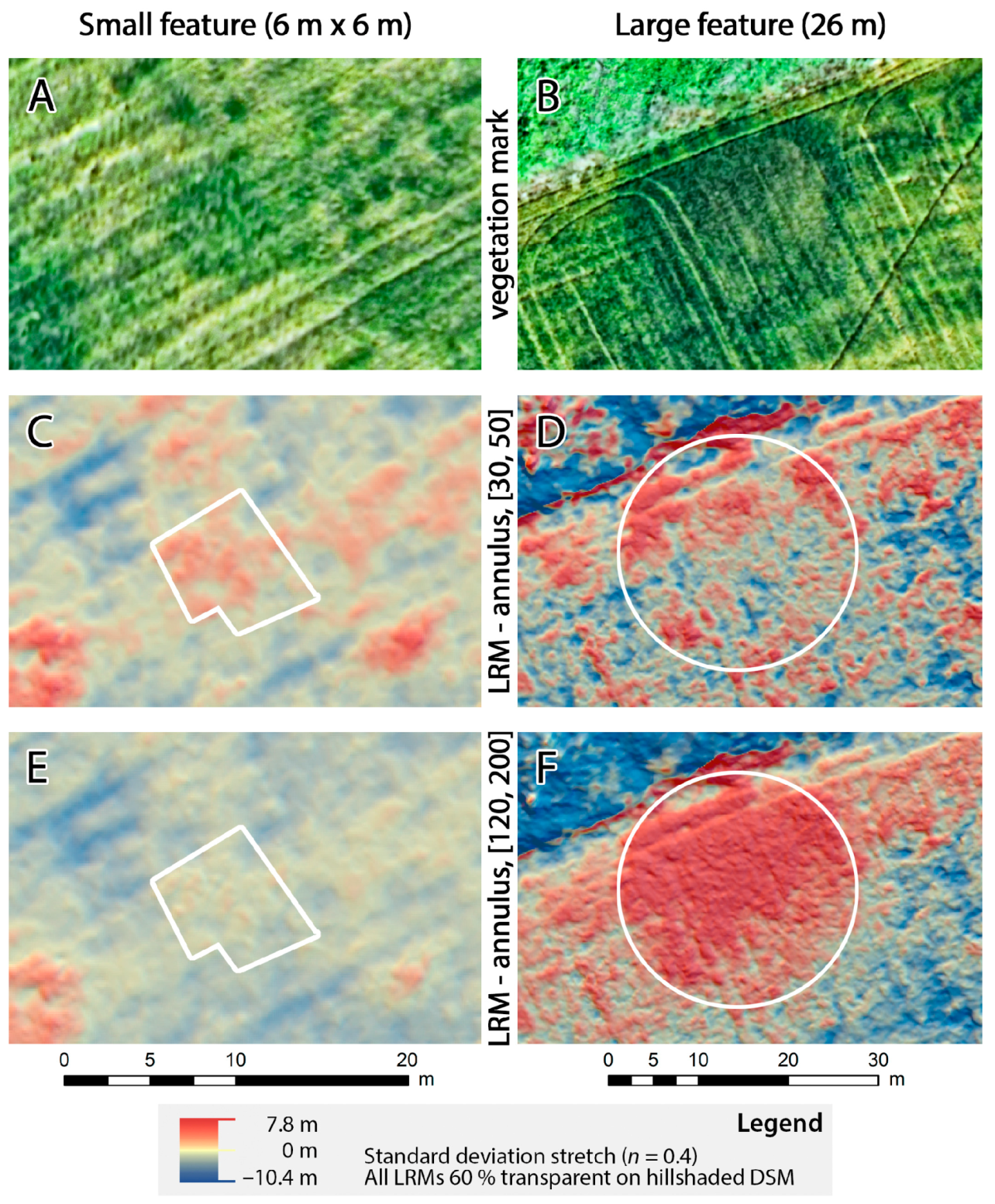
As applies to any kernel-based algorithm, the LRM computation greatly depends on the kernel’s shape and certainly its size (
Figure 3). After some experimentation, the annulus kernel (which is doughnut-shaped) has proven to be very effective (e.g., in handling noise). However, if the diameter of the kernel is too small, very large surface features can remain in the purged DEM. Small kernels will thus highlight smaller features better (e.g.,
Figure 3C), while large kernels tend to remove the smaller features, hereby accentuating the bigger ones (e.g.,
Figure 3F). Moreover, the LRM can, much like any other DEM, be displayed with different colour mappings. Here, a red/yellow/blue diverging palette was used with a standard deviation stretch of
n = 0.4.
4. Interpreting the Canopy
The multitude of layers produced from the data processing and visualisation provided a range of data for subsequent interpretive mapping. Although it is difficult to exhaustively describe the interpretative phase, two examples in
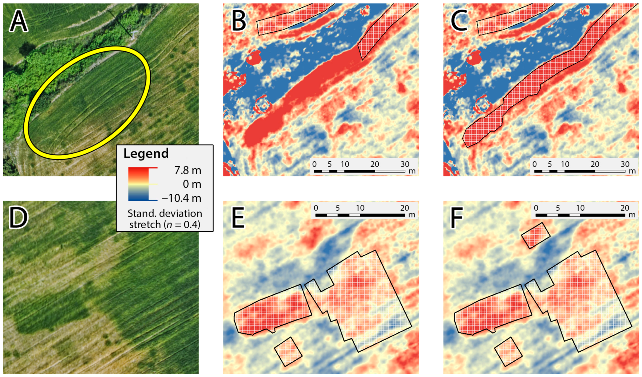
Figure 4 illustrate the complementary nature of these data layers. The initial mapping was based solely on the colour differences discernible in the optimised vegetation orthophotographs.
Figure 4A,B shows that two large ditches could be mapped (amongst many smaller features which are not indicated for illustration clarity). At the end of the lower ditch, a homogenous green area appears. This zone, which is indicated by the ellipse in
Figure 4A, makes it impossible to further trace the ditch. When switching to the LRM generated by an annulus kernel with a size of [45, 75] pixels, the continuation of this ditch is clearly visible due to the higher vegetation which is encoded in red (
Figure 4B). Thanks to this interplay, the ditch was finally traced to nearly the end of the Montarice plateau (
Figure 4C).
A second example is also provided in
Figure 4D–F. Here, the difference between the vigorous green crops and the chlorotic plants as illustrated in the orthophoto allowed for the mapping of three building structures (
Figure 4E; again, the smaller structures are not indicated for illustration clarity). It was, however, only after considering the same LRM that a fourth building structure was noticed (
Figure 4E,F). Although one can argue that this structure is also visible in the orthophoto, the density of the structures on Montarice makes it very easy to overlook smaller or larger features (depending on the map scale one uses to interpret). Being able to visualise another data variable (i.e., plant height instead of colour), has the power to draw the eye to features that otherwise might go unnoticed.
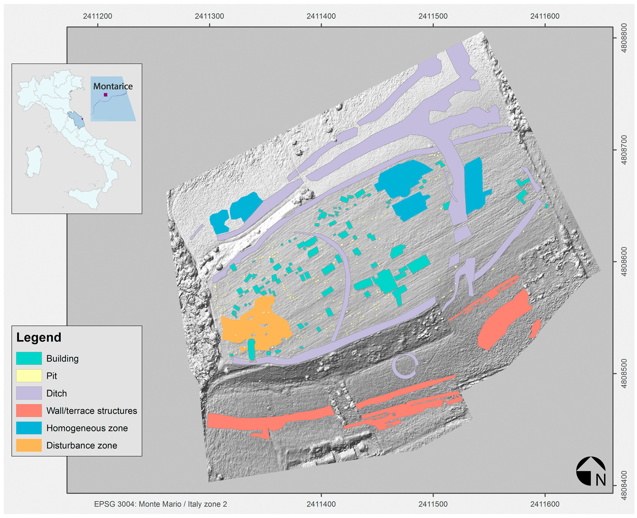
In the end, the consideration of all data layers made it possible to generate an interpretative map of the site (
Figure 5). The positive and negative vegetation marks on the plateau and its northern and southern slopes depict a whole series of linear, round, and more or less amorphous features, although dating and phasing of these structures is currently still impossible. It is likely that rectangular and pseudo-rectangular traces of different size reveal the buried remains of houses or house segments, especially in the western and central parts of the plateau. Throughout the plateau, we can distinguish elements of a minimum of thirty houses and smaller buildings with predominantly rectangular shapes. Many are aligned parallel with or perpendicular to the long sides of the elliptic plateau, which suggests a certain organisation. These probable building traces are interspersed with hundreds of smaller anomalies, possibly pits, larger postholes, and maybe some wells and other activity traces, some of which seem to be aligned and could have formed part of a constellation of wooden houses.
Larger and wider linear features, partly related to the geomorphology of the site, can be interpreted as remains of enclosure ditches, some of which might have been paralleled by a wall or earthwork. Apart from the main ellipsoid ditch system flanking the plateau along its long sides, which may have completely surrounded it at some time, we can also distinguish a remarkable curved central ditch (possibly once surrounding the highest part of the site) and an intricate, wider system cutting the plateau and linking up with a series of ditches and other linear traces on the northern slopes. However, some of these northern systems could also be seen as part of a terracing system just like the parallel ones on the southern slopes. A smaller but very intriguing ditch enclosure could be discussed on the south-central slope of the site: it definitely describes a clear circle and could be interpreted as the remains of a monumental burial site located in a very visible position near the edge of the settlement area (see also
Figure 3B). Finally, certain larger conglomerates of anomalies in the crops might be related to erosion disturbance (on the western plateau top) or to more homogenised areas of human activity or clustered buildings (in northern parts of the site).
5. Discussion and Future Research
This paper has explored the value of extracting a vegetation elevation model from archived aerial photographs and has shown how this new data layer can serve as a proxy to detect archaeologically-induced changes in the soil. Since one no longer has to rely solely on the colour contrasts exhibited by the photograph itself, this novel approach adds serious significance to the use of archaeological aerial imagery. Although it is the first time that aerial photographs have been employed in this way for the identification of vegetation marks, a similar approach was taken by Stott et al. [
30] using ALS-derived CHMs. Even though they did not use the LRM to visualise elevation contrasts, these scholars could demonstrate that in certain situations, the CHM provides better definition of archaeological features than aerial photographs acquired at the same time. Moreover, their approach indicated the importance of vegetation height as a proxy for sub-surface archaeological features in ‘difficult’ clay soils (they are called ‘difficult’ as their imperfect drainage hampers the creation of vegetation marks [
66]).
The spatial resolution of the ALS data was, however, stated as a critical issue, since too large a laser pulse footprint has a strong generalising effect on the resulting CHM. In this aspect, the spatial resolving power of airborne sill cameras and the dense point clouds that can be generated by IBM-pipelines have a clear edge over ALS-based approaches. Furthermore, acquiring aerial imagery has less cost implications than committing an ALS flight. Additionally, this study has shown that an image-based approach can also deal with archived data. Given the multitude of images that are stored in various archives all over the world, the presented approach has the potential to yield multi-temporal CHMs and, as such, access another dimension (i.e., the temporal one) of the canopy. Not being limited solely to the spectral dimension of the vegetation also means that the aerial photography detection window for archaeological features can be extended, while the certainty of feature detection can most likely be increased. Together with many other arguments (see [
40,
67]), both characteristics play directly into the hands of a total coverage aerial reconnaissance approach.
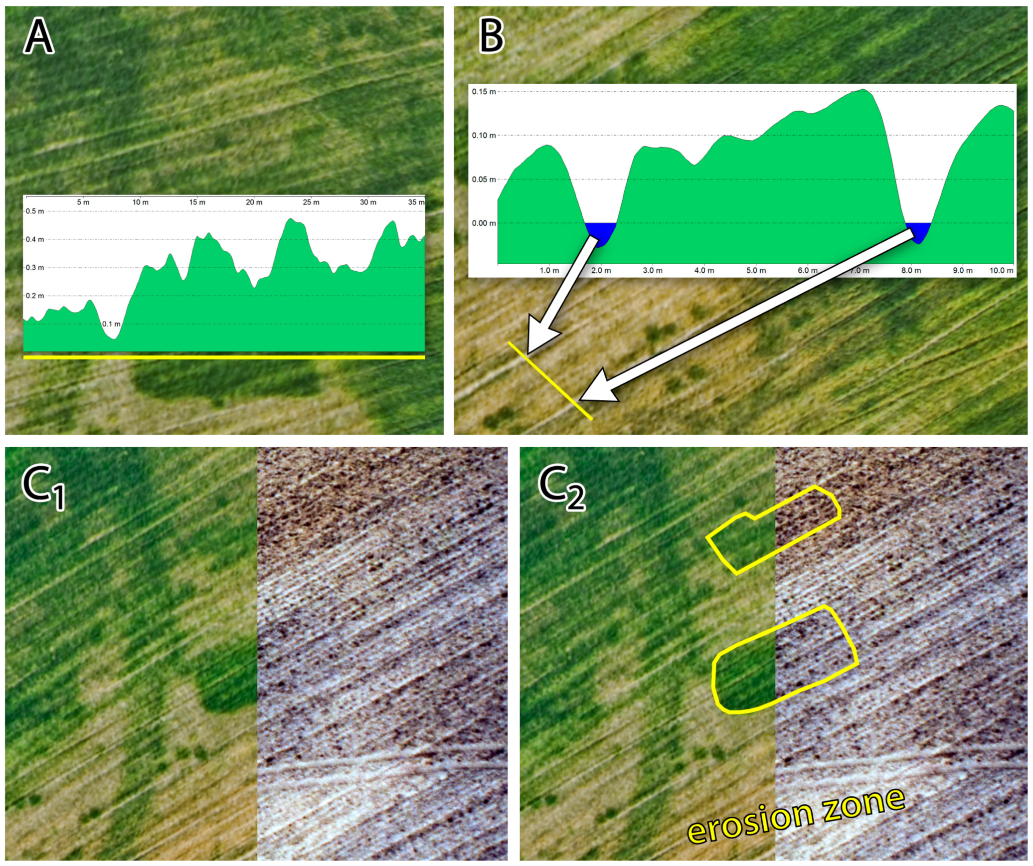
Although the benefits of having perfectly co-registered bare-earth and vegetation surfaces are manifold, obtaining accurate DEMs from non-photogrammetrically scanned archival imagery can be a slow and cumbersome process. Furthermore, the lack of highly accurate ground control data means that the geometrical accuracy of the generated 3D surfaces could also not be thoroughly assessed. However, it is possible to qualitatively validate the CHM when comparing it with the orthophotograph.
Figure 6 shows that the vegetation profile does exactly what one would expect from the distinct photo colours: in longer periods of drought, taller vegetation will largely correspond to the greenness of plants (
Figure 6A) in the absence of senescence as well as acute biotic (pests, weeds, disease, fungi) and abiotic (floods, high light intensity, drought, chilling, mineral deficiency, ozone) constraints [
58].
Figure 6B shows that the chlorotic vegetation is only 10 to 15 centimetres high, while the CHM even reveals small depressions of a few centimetres between the sowing lines. Finally, some areas of the plateau feature a perfect correlation between the soil marks and the vegetation colour (note the central dark green mark that neatly aligns with a darker soil colour in
Figure 6C). All three examples more or less indirectly prove the correct co-registration of the DSM and DTM with few local deformations.
Similarly to the discolouration of vegetation, contrast in vegetation heights (or the lack thereof) will not always correspond to sub-surface archaeological features. This is due to the fact that both vegetation and soil type, together with all possible environmental conditions, play a substantial role in how the canopy properties relate to the buried archaeology [
68]. The success of using the canopy surface and its various visualisations as a suitable method for detecting archaeological features also depends on the terrain and the availability of a bare-earth model that can serve as a baseline. Any undulation in the underlying topography will make the assessment of height differences encoded in a vegetation DSM difficult and error-prone. As such, a bare-earth model is still required for an optimal assessment of the true vegetation height by means of a CHM. Although in most situations one bare-earth reference can be sufficient for analysing subsequent datasets, erosion-sensitive sites such as Montarice will seriously benefit from an approximately contemporary DTM.
In addition to the issues raised above, future research will focus on the image fusion between different data sources. Due to the abundance and variety of remote sensing and geophysical data layers that are generated for a site like this, the need arises for a meaningful combination of all this imagery. For many years, various research fields have been trying to integrate imaging data of different modalities, not least in the geoscience and medical communities, to facilitate a better understanding and interpretation of particular phenomena. Similarly, in the field of archaeology and more specifically archaeological prospection, the constant growth in the number and variety of image acquisition techniques creates an increasing demand for image fusion techniques to be incorporated in the analysis of these data. To test well-established and state-of-the-art image fusion methods and facilitate the development of new data integration routines, a dedicated MATLAB toolbox called TAIFU (the Toolbox for Archaeological Image Fusion) has been created and is constantly expanded [
69]. The Montarice datasets presented here will, together with the aerial imagery from other flights and geophysical imagery, provide an ideal case study for an archaeological assessment of TAIFU and will hopefully enable more trustworthy information extraction and a better interpretation of the hidden geo-cultural landscape.
6. Conclusions
This paper has investigated methods for detecting and accurately mapping archaeological features from archived airborne, visible spectrum photography. More specifically, archival imagery from two observer-directed aerial sorties above the protohistoric hilltop settlement Montarice has been converted into 3D datasets for archaeological analysis. In a first step, the scanned diapositives were processed in an image-based modelling pipeline. Although such computer vision-based approaches are well studied and known to be capable of producing highly accurate surface models, processing archived analogue material is much more error-prone and time-consuming than dealing with newly acquired digital photographs due to complex image distortions and insufficient metadata. Moreover, the ground control, of critical importance to the process, might be difficult to acquire given the landscape changes over time. However, no superior soil and crop mark records of Montarice have since been recorded in the framework of the Potenza Valley Survey. This makes the analogue image sets one of the most valuable visual records collected during the course of the project, and therefore well worth the effort.
Despite these issues, an accurate digital vegetation model and co-registered digital bare-earth model could be obtained from the original imagery. Subsequently, a 2.5D canopy height model was computed using both 3D surfaces. To visualise the small crop differences embedded in this canopy model, several local relief models were calculated. Although the impact of kernel size on the visibility of the features in a local relief model was clearly illustrated, the latter proved to be of the utmost importance in interpreting the vegetation marks visible in the optimised orthophotographs.
Though the meaning of many features, certainly those located on the slopes of the hilltop, is still unclear, this paper has shown that a fuller use of (archived) aerial imagery—through the extraction of height differences and their use as proxies for sub-surface archaeological residues—can expand their utility for archaeological prospection. The current archaeological map of Montarice would never be so detailed solely through the examination of the spectral dimension of the aerial photographs. While the value of accurately positioned orthophotographs generated from archived photographic material is great, the extraction of variation in crop height allows for a new dimension of vegetation mark visualisation and thus a greater engagement with the recorded canopy features.


