Object-Based Change Detection in Urban Areas: The Effects of Segmentation Strategy, Scale, and Feature Space on Unsupervised Methods

Abstract

Object-based change detection (OBCD) has recently been receiving increasing attention as a result of rapid improvements in the resolution of remote sensing data. However, some OBCD issues relating to the segmentation of high-resolution images remain to be explored. For example, segmentation units derived using different segmentation strategies, segmentation scales, feature space, and change detection methods have rarely been assessed. In this study, we have tested four common unsupervised change detection methods using different segmentation strategies and a series of segmentation scale parameters on two WorldView-2 images of urban areas. We have also evaluated the effect of adding extra textural and Normalized Difference Vegetation Index (NDVI) information instead of using only spectral information. Our results indicated that change detection methods performed better at a medium scale than at a fine scale where close to the pixel size. Multivariate Alteration Detection (MAD) always outperformed the other methods tested, at the same confidence level. The overall accuracy appeared to benefit from using a two-date segmentation strategy rather than single-date segmentation. Adding textural and NDVI information appeared to reduce detection accuracy, but the magnitude of this reduction was not consistent across the different unsupervised methods and segmentation strategies. We conclude that a two-date segmentation strategy is useful for change detection in high-resolution imagery, but that the optimization of thresholds is critical for unsupervised change detection methods. Advanced methods need be explored that can take advantage of additional textural or other parameters.

1. Introduction

Information on changes in land use and land cover in urban areas is very important for scientific research into, for example, urban expansion as well as for practical applications such as urban planning and management. For medium (10 m to 100 m) and low (>100 m) resolution remote sensing images [1], typical per pixel change detection methods have been able to meet the requirements for change detection at regional and national levels [2,3,4], but the increasing availability of high spatial resolution data that provide more detailed landscape characterization now allows us to analyse urban areas at a local level [5,6]. However, change detection using high-resolution images faces additional challenges due to, for example, small spurious changes [7], high-accuracy image registration, and shadows resulting from different viewing angles [6,8] (which can be dominant in urban areas). Fortunately, these effects are reduced by using object-based approaches rather than pixel-based approaches, as has been demonstrated by many previous researchers [8,9,10].

Object-based image analysis techniques have recently been more frequently used for change detection at local levels due to their distinct advantage in overcoming the “salt and pepper” effect of using high-resolution imagery [3,11,12,13]. However, assessing the effect that the segmentation scale has on object-based change detection is a crucial aspect of any particular study [14], when it has been considered to be a key factor in object-based classification [15,16]. Furthermore, a methodological challenge faced in the use of an object-based paradigm is whether or not the segmented objects generated by two-date datasets are perfectly matched [14], since post-classification comparisons are very popular in change detection [17,18]. In this study we therefore focus on pre-classification change detection (only identifying “change” or “no change”, and not the type of change [10]), which generates consistent objects across multi-temporal imageries, in contrast to post-classification comparisons in which spatial matches between independent segmented objects from two-date datasets are difficult to establish due either to changes in the objects or to uncertainties in the segmentation [7]. For pre-classification, typical segmentation strategies based on the input bands can be grouped into two classes: image-object overlay (IOO) strategies in which a second image is overlain directly on objects segmented from one of the multi-date images for comparison, and multi-temporal image-object (MTIO) strategies in which images in the entire time series are segmented together [18]. Although Tewkesbury et al. suggested that MTIO units of analysis might be the most robust, they also indicated that further investigation is warranted into the use of units of analysis derived from different segmentation strategies for object-based change detection [18].

Numerous investigations have demonstrated the use of unsupervised change detection techniques within object-based workflows [12,13,19,20,21,22,23], including the use of Multivariate Alteration Detection (MAD) [12], Principal Component Analysis (PCA) [24], object multidate signatures [19,20], and direct detection of differences without feature transformation [23]. However, none of these investigations provide coherent guidance on the effect of different change detection processes because comprehensive assessment of such processes is challenging due to the uncertainty in object sizes, the complexity of segmentation strategies, the diversity of change detection techniques, difficulties in threshold selection, and the numerous features available [24,25,26]. In their review, Tewkesbury et al. called for further investigations into the different methods and units of analysis used [18].

In order to address these problems, we concentrated our investigations on object-based pre-classification change detection and primarily assessed commonly-used unsupervised change detection techniques within a number of different segmentation strategies by varying the segmentation scales, thresholds, and features. This kind of systematic analysis had not previously been attempted and provided an opportunity to synthesize the results obtained from different change detection processes, allowing us to compare their performances using different segmentation scales, segmentation methods and features that might affect our ability to detect change. Since this evaluation seemed to be urgent according to previous review by Tewkesbury et al. [18], it was only conducted for urban area in this study. Further experiments are needed for a universal recommendation, but our results are a first step to help practitioners decide which change detection technique to use, to understand how the factors investigated affect the change detection accuracy, and to clearly conclude which analysis unit will be the more robust for their particular purposes.

2. Study Areas

The study concentrated on two areas within the city of Changzhou, China, where land use and land cover are changing rapidly with development of the Yangtze River delta region (Figure 1). For our research, we used two Ortho Ready Standard Level-2A bundles of WorldView-2 (WV2) images acquired on 31 December 2009 and 12 December 2013. Each image consisted of four 2 m multispectral bands (e.g., red, blue, green and NIR) and one 0.5 m panchromatic band.

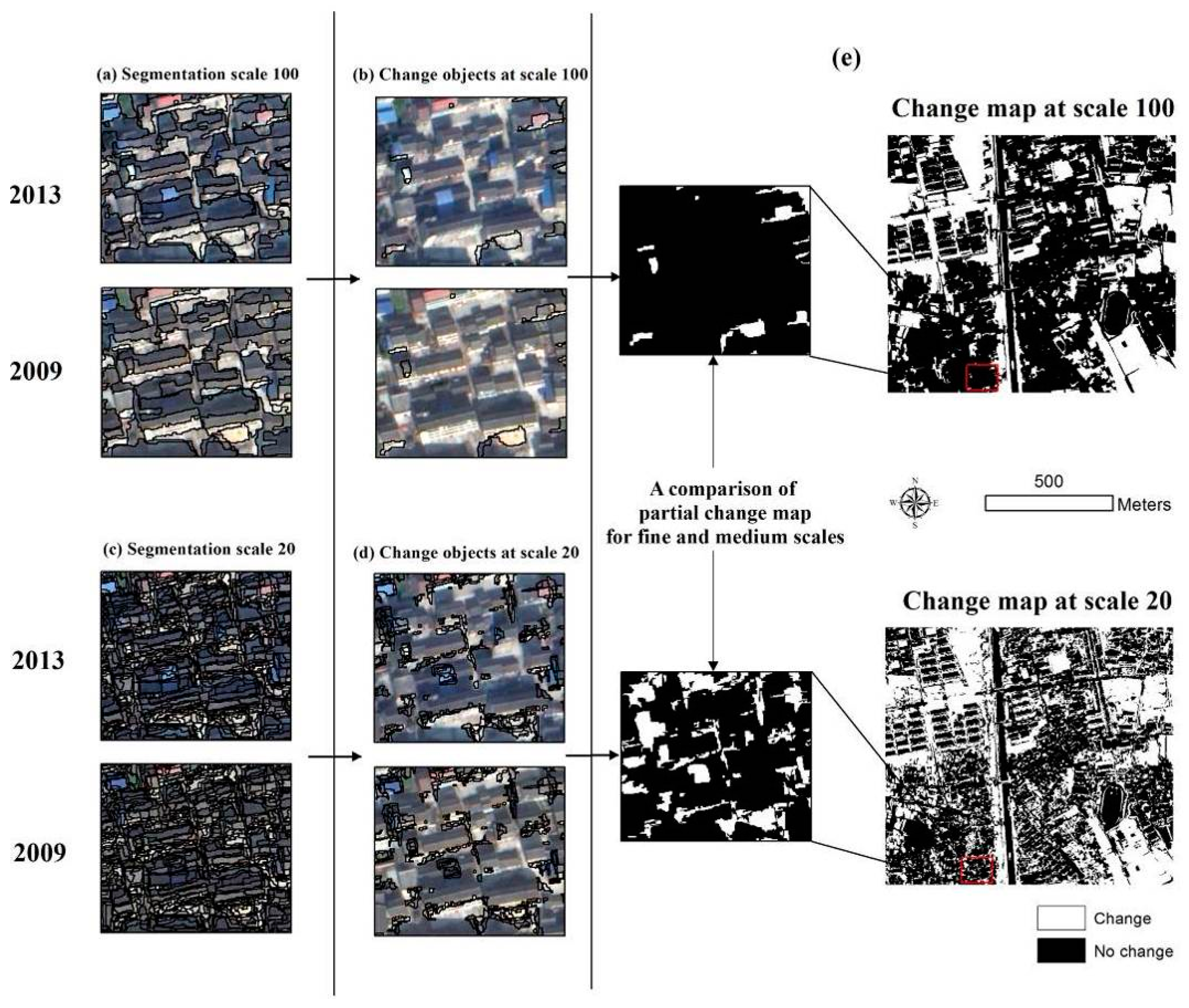
3. Methods

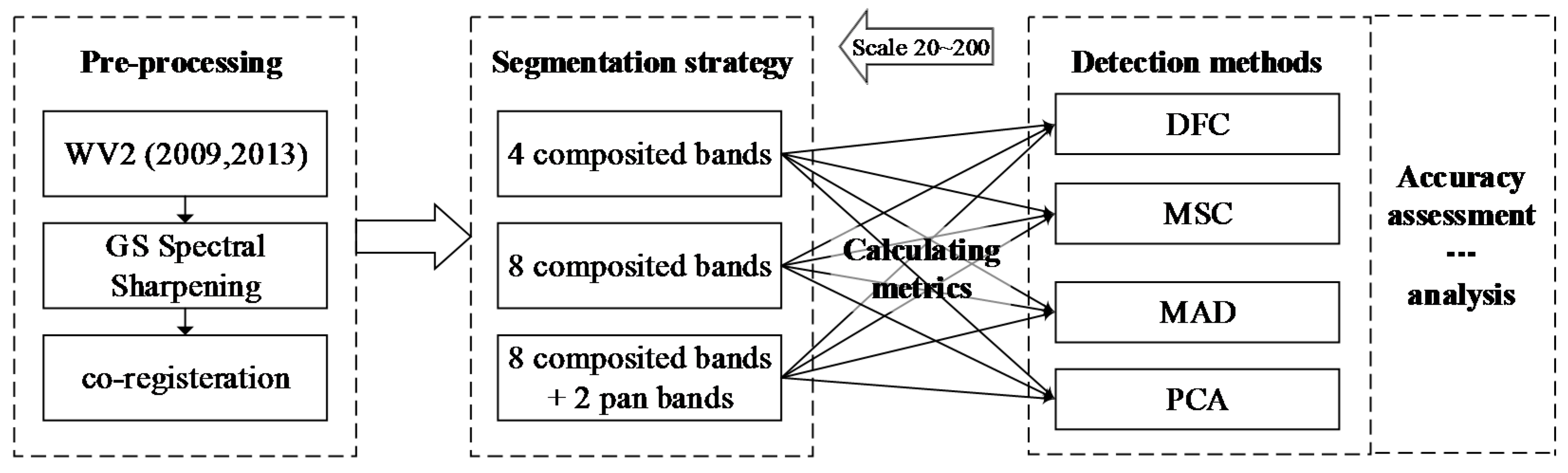
The workflow used to systematically assess the factors affecting object-based processes involved four steps, as shown in Figure 2. The first step involved data pre-processing to generate registered, pan-sharpened image stacks ready for subsequent processing [27]. In the second step, multiresolution segmentation [28] was applied separately to a number of different band combinations to generate a variety of different units of analysis even at the same scale (see Figure 2). In the third step, in order to identify changed objects using feature information (see Section 3.3), chi-square transformation [13], which has been widely used in object-based change detection workflows, was applied to a number of different feature difference signatures. Four methods were applied, including original features (Direct Feature differentiation based chi-square transformation (DFC)), MAD variates [12], the first three PCA components [24], and object multidate signatures (Mean and Standard deviation signature based chi-square transformation (MSC)). As the fourth step, a polygon-based accuracy assessment method was used to calculate the error matrix [29]. This process was repeated for each segmentation scale and each threshold applied to the chi-square statistic, resulting in different detection accuracies under different conditions. Finally, we also evaluated how additional basic textural and Normalized Difference Vegetation Index (NDVI) information affect the change detection performance on the investigated unsupervised methods.

3.1. Data Pre-Processing

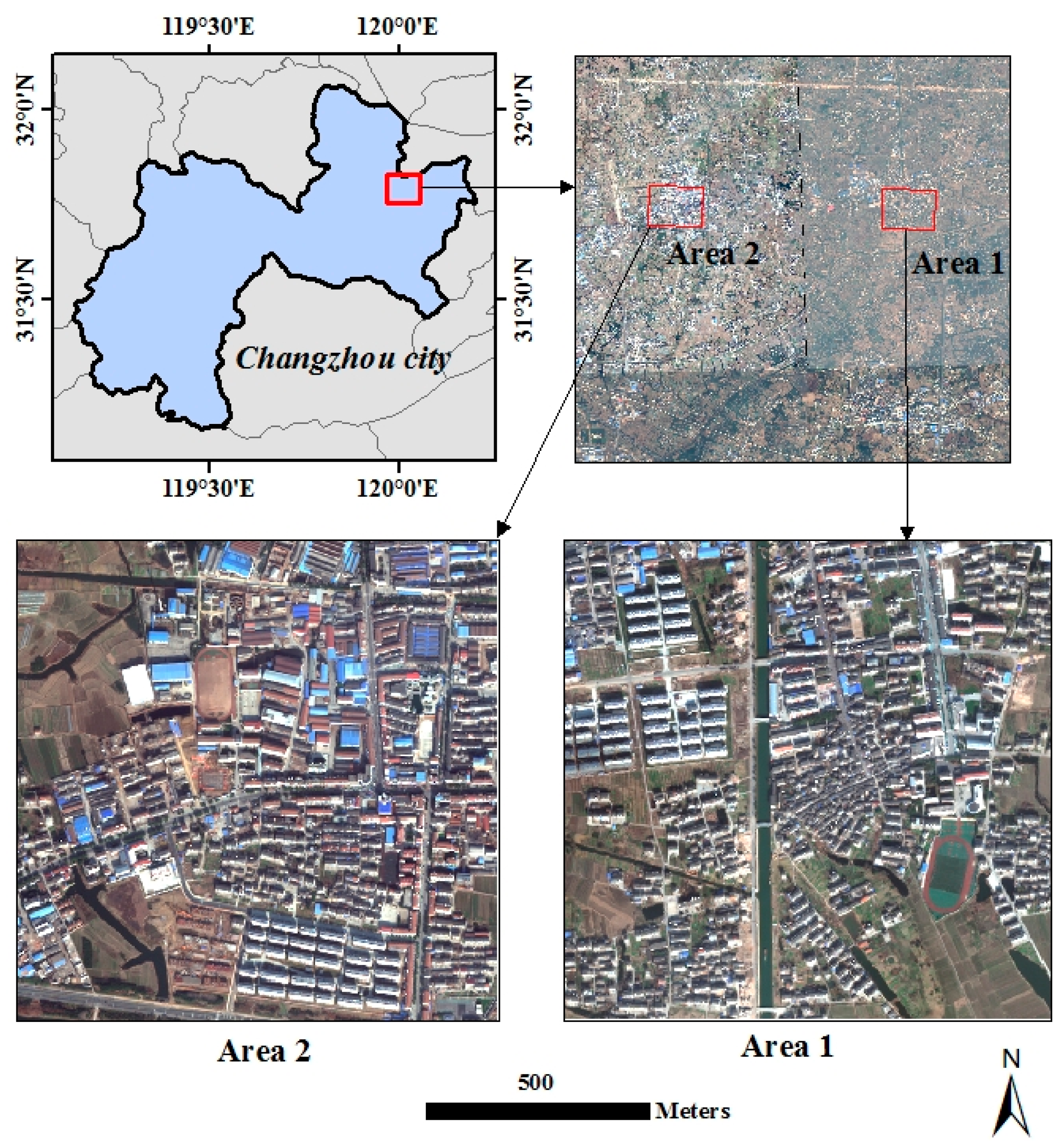
The Gram–Schmidt (GS) algorithm was used to fuse the panchromatic band with the multispectral bands [27,30,31], resulting in pan-sharpened 0.5 m resolution images, which were used in the following analyses. For our investigations, we extracted two subsets of the WV2 imagery to cover two areas of similar extent: Study site 1 covering 1128 × 1010 m and Study site 2 covering 1130 × 1012 m (Figure 1). Each of these subsets (hereafter, image pairs) was processed separately using the following steps, including image registration and relative radiometric normalization. The 2009 imagery was first automatically registered to the 2013 imagery using the second-order affine polynomial and the nearest-neighbour resampling method in ENVI 5.0 (Exelis Visual Information Solutions, Boulder, CO, USA), resulting in a registration error (root mean square error) of less than 1 m (2 pixels), which is an acceptable error range for high resolution imagery [32,33]. In order to match the spectral responses of the two-date images, relative radiometric normalization (histogram matching) was then implemented using the image pair with the largest spectral variance as the reference images. Two-date images were then loaded into eCognition software 8.7 (Trimble Geospatial, Munich, Germany) in order to perform segmentation using the different segmentation strategies.

3.2. Multiresolution Segmentation

In order to ensure a strict separation of analysis units, we followed three strategies for segmentation using a multiresolution segmentation algorithm [28], as implemented in the eCognition software package, with segmentation scales ranging from 20 to 200 at intervals of 10. We first imported 8 pan-sharpened (composited multi-spectral (MS)) bands and 2 original panchromatic bands of the two different dates into the eCognition software and then implemented three segmentation strategies in eCognition, assigning different weightings to each of the input bands (i.e., 0 or 1, with bands involved in segmentation processes assigned a weighting of 1 and those not involved in segmentation processes assigned a weighting of 0). In Strategy 1, the IOO method as mentioned above, only 4 pan-sharpened bands from the 2013 image were input for the image segmentation (the weightings for pan-sharpened MS bands in 2013 were set to 1 and for the others to 0). In Strategy 2, the image segmentation process was performed for a total of 8 pan-sharpened bands from the bi-temporal image datasets (the weightings for the pan-sharpened MS bands were set to 1 and those for the two panchromatic bands to 0). In Strategy 3, image segmentation was conducted from the stacked images for a total of 8 pan-sharpenend bands plus 2 panchromatic bands (an equal weighting was assigned to each of the input bands), since the panchromatic bands possibly contained more detailed textural information. Both Strategies 2 and 3 are MTIO methods as defined in the introduction. For all three of the strategies, the features from the 2009 and 2013 images were then calculated based on the same objects for change comparison. The different weightings on the input bands for segmentation meant that different units derived from different segmentation strategies could be produced for further change detection analysis, in order to explore the best segmentation strategy. Multiresolution segmentation typically optimizes the object homogeneity (which is determined by the compactness parameter) using the colour weighting in addition to the shape weighting. Previous research has suggested that a higher colour weighting yields better segmentation results as it gives greater emphasis to spectral information [15,34]. The colour and shape parameters were therefore set to 0.9 and 0.1, respectively, in this study. Both smoothness and compactness were assigned the same weighting (0.5) in order to avoid the bias introduced by compact or non-compact segments [15,35].

3.3. Feature Calculation

Object size and shape features could not be compared between two-date images using IOO or MTIO segmentation strategies due to the consistent segmented objects obtained for both dates [18]. We therefore calculated a number of spectral and texture features, together with NDVI values, for our study, rather than using meaningless geometric features. An NDVI band was calculated for each pixel as the difference between the near-infrared and red bands divided by their sum [36]. The spectral and NDVI parameters for each object were generated by calculating the means from the four multispectral bands and the NDVI band. In addition, four textural parameters (gray-level co-occurrence matrix (GLCM) homogeneity, GLCM angular second moment, GLCM mean, and GLCM entropy) that have been shown to be important for object-based classification [15,34] were derived from individual panchromatic bands because we wanted to retain original textural information and avoid any compositing effect.

3.4. Identifying Changed Objects Using Four Different Methods

Differentiating between images for OBCD, based on a pair of co-registered images, was performed through object-by-object rather than pixel-by-pixel comparisons, using object statistics (spectral mean values per object). The chi-square transformation has previously been applied to remote sensing change detection and has proved to be efficient at detecting both per pixel and per object changes [2,37]. In this study, we used four common methods based on a chi-square transformation for the recognition of changed objects because of the advantage that this offered of simultaneously taking into account multiple variables, as reported in previous reviews [2]. Each method was applied repeatedly in order to detect any changes in objects, using various parameters (e.g., segmentation scale and confidence level 1-$\alpha$) in order to evaluate the effects that they have on change detection accuracy. Although these methods have been widely used in previous studies for a variety of applications, they have often been presented with different names due to the flexibility of the multivariate statistical techniques. As in some of these previous studies, we also used some variables derived by PCA and MAD in addition to the direct spectral and textural features. We named these methods Direct Feature differentiation based chi-square transformation (DFC), Mean and Standard deviation signature based chi-square transformation (MSC), PCA based chi-square transformation, and MAD variates based chi-square transformation (

Table 1. Four input differencing variables and their chi-square transformations, and the respective mean Mahalanobis number (Mn). Detailed explanations can be found in Section 3.4.1, Section 3.4.2, Section 3.4.3 and Section 3.4.4.

Method	Difference	Detection Value	Distribution
DFC	Original features difference $X$	Chi square (Mn)	${\chi }^2\left(p\right)$
MSC	$X_i={\left(M_{i1},\cdots ,M_{ib},S_{i1},\cdots ,S_{ib}\right)}^T$	Chi square (Mn)	${\chi }^2\left(2p\right)$
MAD	$MA{D}_i=a^{T}X-b^{T}Y$	${{\displaystyle \sum _{i=1}^p\left(\frac{MA{D}_{ij}}{{\sigma }_{MA{D}_i}}\right)}}^2$	${\chi }^2\left(p\right)$
PCA	PCA—first 3 components	Chi square (Mn)	${\chi }^2\left(3\right)$

Abbreviations used in this table: DFC: Direct Feature differentiation based chi-square transformation; MSC: Mean and Standard deviation signature based chi-square transformation; MAD: Multivariate Alteration Detection; PCA: Principal Component Analysis.

). A detailed summary of four methods is provided from Section 3.4.1 to Section 3.4.4.

3.4.1. DFC

For direct differentiation of features, we used the original features of the objects without any feature transformation for the DFC method. We defined the digital value of the object in the “changed” dataset (Mahalanobis number (Mn)) as $Y$, the vector of the difference between all of the features considered between the two dates for each object as $X$, the vector of the mean residuals of each feature as $M$, the transposition of the matrix as $T$, and the inverse covariance matrix of all features considered between the two dates as ${\displaystyle \sum {}^{-1}}$. We then define a chi-square transformation formula as

$$Y={\left(X-M\right)}^T{\displaystyle {\sum }^{-1}\left(X-M\right)}$$

(1)

where $Y$ is distributed as a chi-square random variable with p degrees of freedom and p is the number of variables [2]. We can then write that

$$P\left(Y_i<{\chi }_{1-\alpha }^2\left(p\right)\right)=1-\alpha$$

(2)

where the value of ${\chi }_{1-\alpha }^2\left(p\right)$ is the changed/unchanged threshold (which can be directly acquired by referring to the chi-square distribution table [2,23]), and the object $O_i$ is labelled as “changed” only when $Y_i$ exceeds this threshold. The Mahalanobis number for the object $O_i$, which is termed $Y_i$, is in this study considered to exceed the threshold ${\chi }_{1-\alpha }^2\left(p\right)$ with a confidence level of $1-\alpha$.

3.4.2. MAD

We also tested the Multivariate Alteration Detection (MAD) technique, which has often been used for per-pixel change detection [38,39,40,41] and also recently for segmented object recognition [12]. Given two multivariate images with variables at a given segmented object written as $X={[X_1\cdots X_p]}^T$ and $Y={[Y_1\cdots Y_p]}^T$, then difference D between the images is simply defined as $a^{T}X-b^{T}Y$, and the $a^T$ and $b^T$ are a set of coefficients from a standard canonical correlation analysis [41], in order to determine the linear combinations of X and Y with maximum variance (corresponding to minimum correlation). Therefore, MAD first calculates the canonical variates ($a^{T}X$ and $b^{T}Y$) and subtracts them from each other, as in Equation (3), and then uses these canonical variates instead of the original features. The MAD variates are linear combinations of the measured variables and will therefore have an approximately Gaussian distribution because of the Central Limit Theorem [41]. The dispersion matrix of the MAD variates [39] is

$$MA{D}_i=a^{T}X-b^{T}Y$$

(3)

where MAD variates are orthogonal with respect to variance [40,41]

$${\alpha }_{MA{D}_i}^2=2\left(1-{\rho }_{p-i+1}\right)$$

(4)

where $\rho$ are eigenvectors of canonical coefficients. Assuming that the orthogonal MAD variates are independent, we can expect that the sum of the squared MAD variates, with standardization to unit variance for object j, will approximately follow a ${\chi }^2$ distribution with $\rho$ degrees of freedom [41]. This can be expressed as

$$T_j={{\displaystyle \sum _{i=1}^p\left(\frac{MA{D}_{ij}}{{\alpha }_{MA{D}_i}}\right)}}^2\in {\chi }^2\left(p\right)$$

(5)

Similarly, we can label the object j as “changed” if the observed $T_j$ value exceeds the threshold ${\chi }^2\left(p\right)$ with a specific confidence level of $1-\alpha$. Here, $T_j$ actually refers to the Mahalanobis number, as in Equation (1), with the only difference being that the input vector consists of MAD variates instead of the original features of the objects.

3.4.3. MSC

Desclée et al. [19] and Bontemps et al. [20] developed a similar method using a chi-square transformation, which, in this study, we refer to as a mean and standard deviation signature based chi-square transformation (MSC). For this method, the mean (M) and standard deviation (S), corresponding, respectively, to measures of feature difference and heterogeneity, were calculated for use as an input signature instead of using a direct input of the original feature difference, in order to improve the change detection capability [19]. The multiple-date signature $X_i$ of each object is then defined as

$$X_i={\left(M_{i1},\cdots ,M_{ib},S_{i1},\cdots ,S_{ib}\right)}^T$$

(6)

where b indicates the number of features, i is the object number, $M_{ib}$ is the mean of feature b for object i, and $S_{ib}$ is the standard deviation of feature b for object i. The same chi-square transformation formula (Equation (1) in Section 3.4.1) was used to compute the Mahalanobis number $C$ using the multiple-date signature $X_i$ (which is chi-square distributed with 2b degrees of freedom [19], because of the extra difference in standard deviations). Thus, for a confidence level of $1-\alpha$.

$$P\left(C_i<{\chi }_{1-\alpha }^2\left(2b\right)\right)=1-\alpha$$

(7)

The “changed”/”unchanged” threshold, therefore, becomes ${\chi }_{1-\alpha }^2\left(2b\right)$ [13].

3.4.4. PCA

PCA is another data transformation method; it converts a set of interrelated variables into uncorrelated variables through orthogonal transformation to reduce the dimensionality of the data, and has been widely used in remote sensing to detect changes in a variety of ways [24,42,43]. A correlation matrix of data variables is first calculated and the eigenvectors and eigenvalues of the correlation matrix are then computed in order to find the principal components [44]. A principle component is generally defined as the eigenvector with the highest eigenvalue, which indicates the greatest variation. The eigenvectors are ordered by eigenvalues, from the highest to the lowest, and the components with lower eigenvalues and hence low significance can be ignored. We applied standardized PCA to the differencing feature vector of the object, thus reducing the dimensionality of a data set while as far as possible retaining any variation [43]. The first three components from the whole data set, which were generally considered to retain most of the information, were then selected as input variables for calculating the Mahalanobis number so that changed objects could be automatically detected. Following chi-square transformation, the Mahalanobis number derived from Equation (1) follows a ${\chi }^2$ distribution, with 3 degrees of freedom.

3.5. Accuracy Assessment

In this study, manual interpretation was used to recognize true change/no change polygons for further assessing the performance of the change detection comparison, and the area was delineated as a true change polygon when visual difference of colour or texture was significant between both date images. We assessed the four described common unsupervised change detection methods in terms of their overall accuracy, sensitivity, and specificity, which were derived from an error matrix calculating by the areal proportions [29]. The performances of the different change detection methods and segmentation strategies were compared at 19 image segmentation scales for 5 confidence levels (i.e., 0.90, 0.95, 0.975, 0.99 and 0.995) on the basis of their overall accuracy by calculating the proportion of the total area that was correctly identified as either “changed” or “unchanged” [45]. Given the reference R with m + n polygons {R₁, R₂, …, R_m+n} and labelled segmentation objects S, the accuracy measures are calculated by matching {S_i} to each reference object R_i. The overall accuracy is defined as:

$$Overall accuracy=\frac{{\displaystyle \sum _{i=1}^m{\displaystyle \sum _{j=1}\left|R_{change\_i}\cap S_{change\_j}\right|}}+{\displaystyle \sum _{i=1}^n{\displaystyle \sum _{j=1}\left|R_{nochange\_i}\cap S_{nochange\_j}\right|}}}{{\displaystyle \sum _{i=1}^{m+n}\left|R_i\right|}}$$

(8)

where m denotes the number of true change polygons in reference layer; n is the number of true no change polygons in reference layer; $|*|$ denotes overlapping area; $R_{change\_i}$ indicates i-th true change polygon in reference layer; $S_{change\_j}$ denotes j-th recognized change object overlaying with i-th true change polygon $R_{change\_i}$; $R_{nochange\_i}$ indicates i-th true no change polygon in reference layer; and $S_{nochange\_j}$ denotes j_th recognized no change object overlaying with i-th true no change polygon $R_{nochange\_i}$.

In addition to the overall accuracy, the accuracy of a binary classification is often described in terms of sensitivity and specificity [46]. The sensitivity is the proportion of an area for which a detection method correctly identifies change, while the specificity is the proportion of an unchanged area that is correctly identified as such [46]. They are defined as:

$$Sensitivity=\frac{{\displaystyle \sum _{i=1}^m{\displaystyle \sum _{j=1}\left|R_{change\_i}\cap S_{change\_j}\right|}}}{{\displaystyle \sum _{i=1}^m\left|R_i\right|}}$$

(9)

$$Specificity=\frac{{\displaystyle \sum _{i=1}^n{\displaystyle \sum _{j=1}\left|R_{nochange\_i}\cap S_{nochange\_j}\right|}}}{{\displaystyle \sum _{i=1}^n\left|R_i\right|}}$$

(10)

and, for explanation, see Equation (8).

We therefore also calculated the sensitivity and specificity at each segmentation scale using different change detection methods and segmentation strategies, in order to explore the relationship between sensitivity and specificity. Finally, we compared the performance of the different change detection methods and segmentation strategies, with and without adding textural and NDVI information.

4. Results

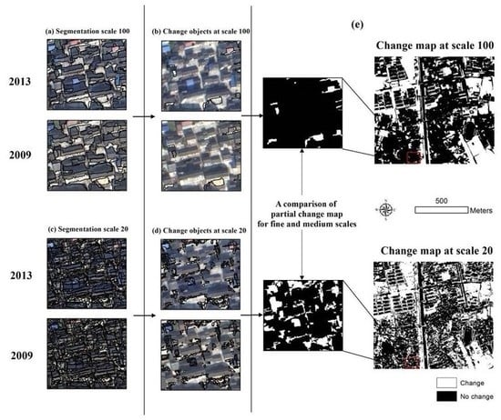
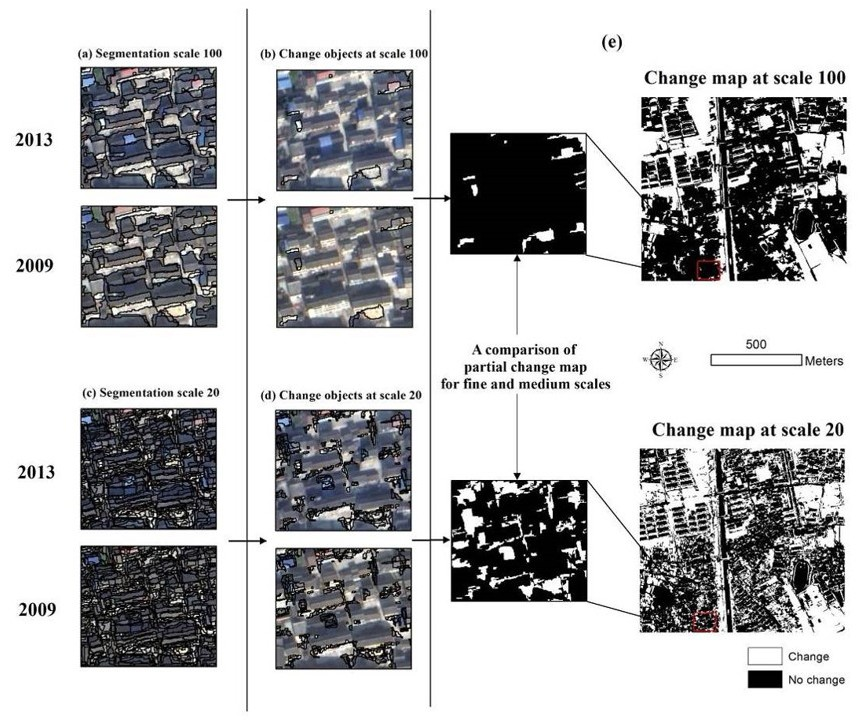
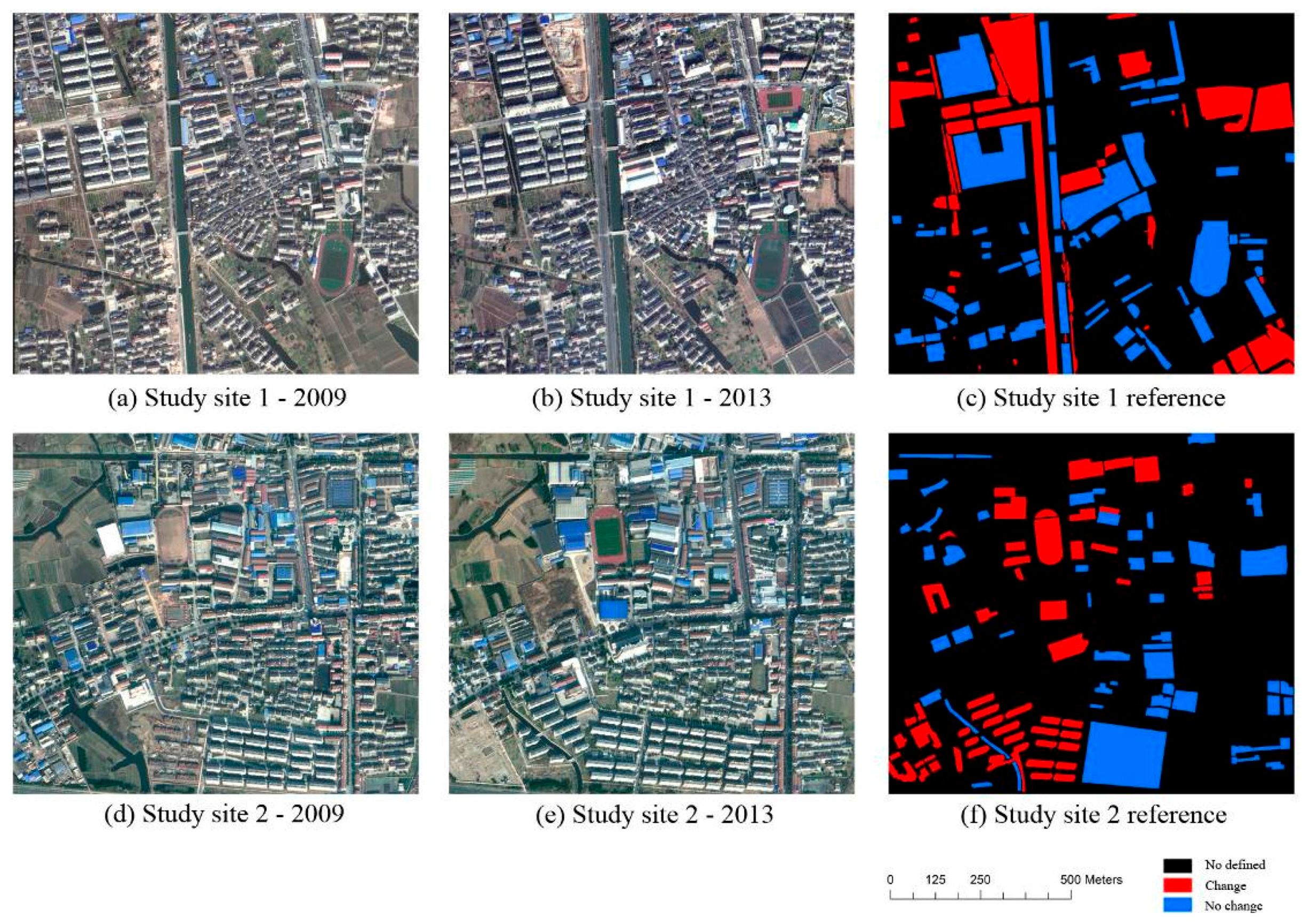
The primary aim of this study was to investigate the effects that segmentation strategies, commonly used supervised change detection techniques, segmentation scale, and feature space have on object-based frameworks. The images (a), (b), (d), and (e) in Figure 3 show two-date composited images for both urban study sites, while (c) and (f) are reference maps from manual interpretation, which only show either “change” or “no change” but do not specify the type of change because of the use of the unsupervised methodology. Based on previous assumption by Foody [46] that the prevalence of change (the amount of change in the confusion matrix) had an impact on the accuracy of results, Foody found that a balance between sensitivity and specificity was generally achieved at a prevalence of approximately 50% [46]. On the basis of our specified accuracy objectives [29], we chose almost equal areas of “change” and “no change” as reference polygons for validation (14.08 ha of “change” and 17.16 ha of “no change” for Study site 1, and 9.02 ha of “change” and 11.32 ha of “no change” for Study site 2), when delineating the changed and unchanged areas within the very high resolution images by manual interpretation.

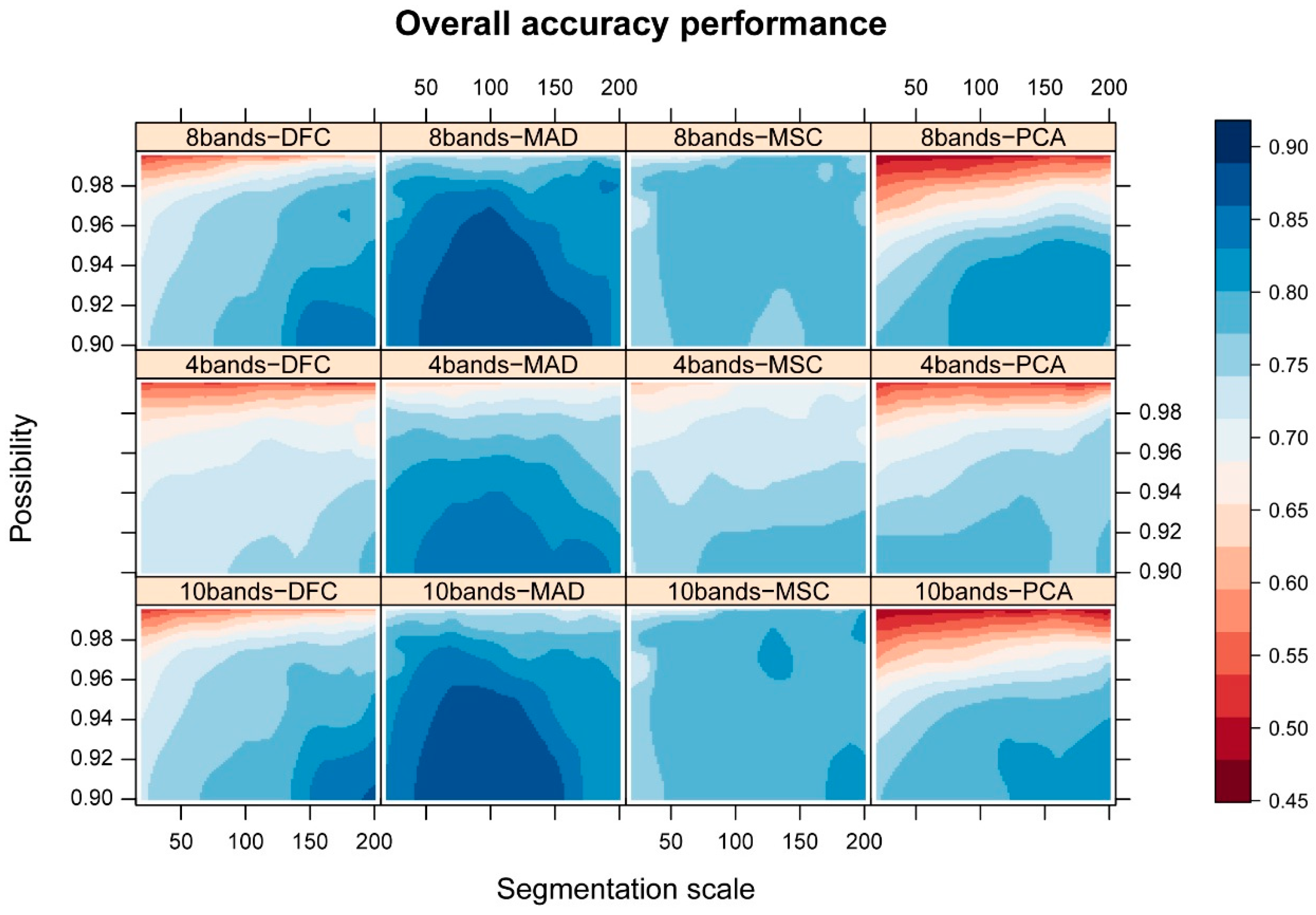
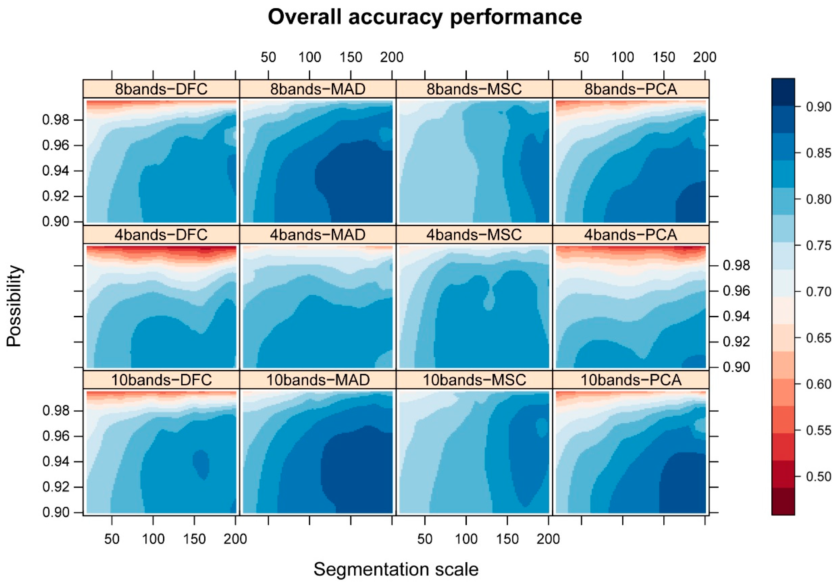
4.1. Responses of Detection Accuracy to Segmentation Strategy and Scale

The effects that different segmentation strategies and segmentation scales had on the overall detection accuracy of four unsupervised change detection methods are summarized in Figure 4 and Figure 5, for both urban areas. Similar patterns of change in overall accuracy with increasing segmentation scale and increasing confidence level were observed for segmentation strategies that used either eight pan-sharpened bands combination or eight pan-sharpened bands +2 panchromatic bands combination (at segmentation scales from 20 to 200). The overall accuracy for the segmentation strategy that used four bands appeared to be lower than that for the other two segmentation strategies, at the same confidence level and segmentation scale. This may be attributable to the fact that the strategies that used eight bands or 10 bands generally yielded smaller objects and any change was therefore more significant for these objects. Irrespective of the unsupervised change detection method employed, the results also suggested that the change detection method that used a four-band segmentation strategy would require a lower confidence level to achieve a comparable detection accuracy to the other two strategies (see Figure 4 and Figure 5). Our results also showed that the overall detection accuracy was sensitive to changes in the segmentation scale, for all of the tested methods. The overall accuracy in all four change detection methods increased rapidly with an increase in the segmentation scale from fine to medium, followed by a more gradual increase (or even a decrease in some cases) with further increases in scale (for example, a decrease occurred at a scale of about 100 using the MAD change detection method).

In addition to the factors discussed above, the relationship between change detection accuracy and confidence level was also investigated by generating separate “changed” images at five different confidence levels (i.e., 0.995, 0.99, 0.975, 0.95 and 0.9). The results indicated that the overall accuracy of all of the unsupervised change detection methods considered increased by different amounts as the confidence level was reduced. A rapid increase in overall accuracy generally occurred between confidence levels of 0.995 and 0.95: the overall accuracy at confidence levels below 0.95 remained relatively stable compared to the overall accuracy at higher confidence levels. There were, however, very large differences between the accuracy levels of the four change detection methods when using the same parameters (i.e., the same confidence levels, segmentation scales, and segmentation strategies). Comparisons between the four change detection methods indicated that MAD outperformed all of the other methods tested, especially when a medium segmentation scale was used (for example, a scale of 100).

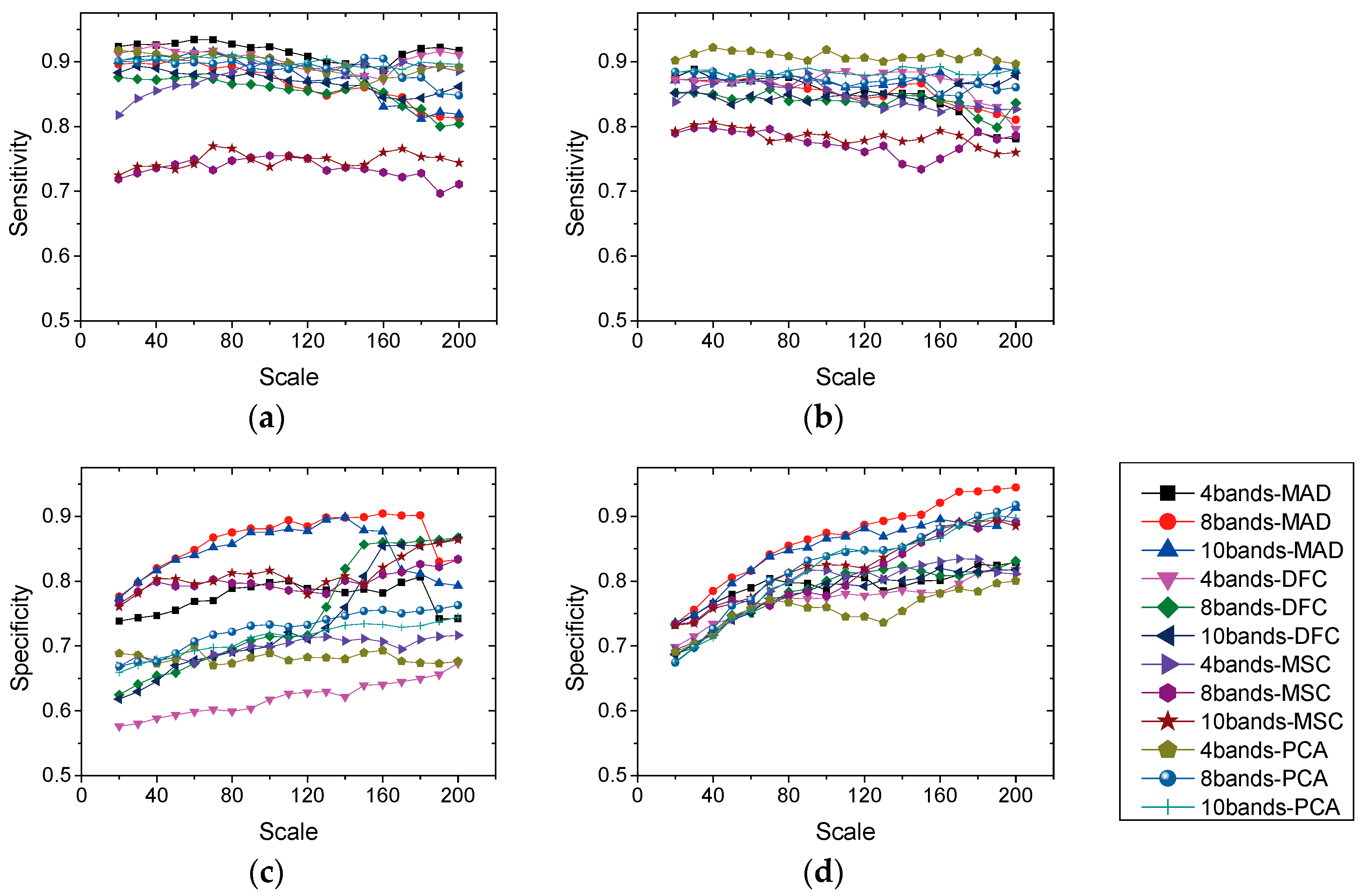
4.2. Relationship between Sensitivity and Specificity

We evaluated the relationship between sensitivity (true positive—change) and specificity (true negative—no change) using a fixed confidence level of 0.9, at which the best overall accuracy was likely to be observed using the same segmentation scales and strategies, as shown in Figure 4 and Figure 5. The results revealed a slight decrease in sensitivity as the segmentation scale increased (Figure 6a,b), while the specificity increased rapidly (Figure 6c,d). The sensitivity thus appeared to be less influenced by segmentation scale than the specificity. In addition, the sensitivity when using two-date segmentation strategies was lower than that when using single-date segmentation strategies. Note that, for each segmentation scale, the lowest sensitivity was observed for two-date segmentation using the MSC method and this was 10% lower than that for single-date segmentation (Figure 6a,b). In contrast, two-date segmentation strategies with eight bands or 10 bands had consistently higher specificities at most segmentation scales than single-date segmentation strategies with four bands. Unlike single-date segmentation, similar patterns of change were observed in the sensitivity and specificity at different segmentation scales for both spectral and spectral-plus-PAN (PANchromatic) two-date segmentation (Figure 6c,d). Figure 6c,d also show that MAD had better specificity than the other methods considered, while PCA frequently had slighter higher sensitivity.

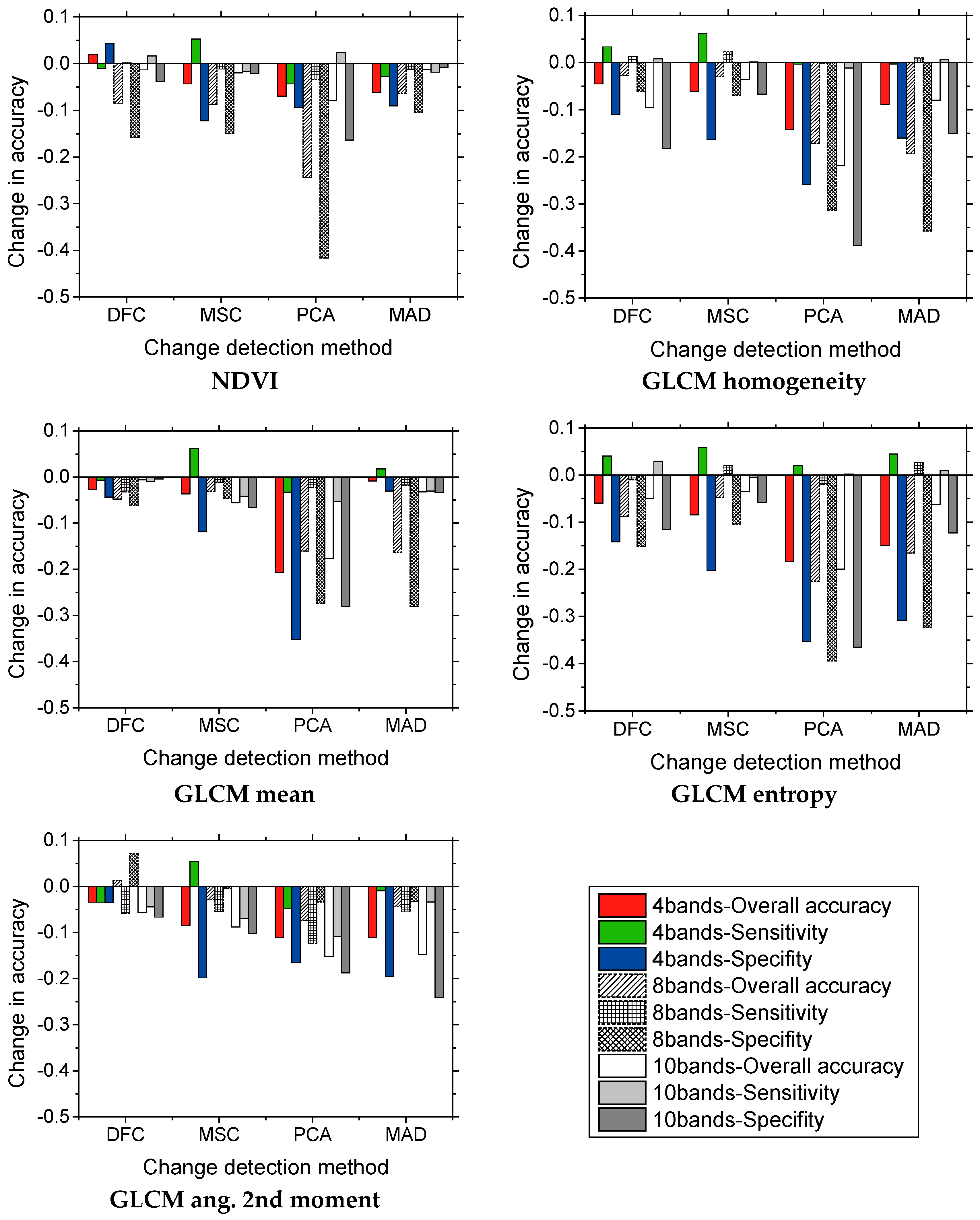
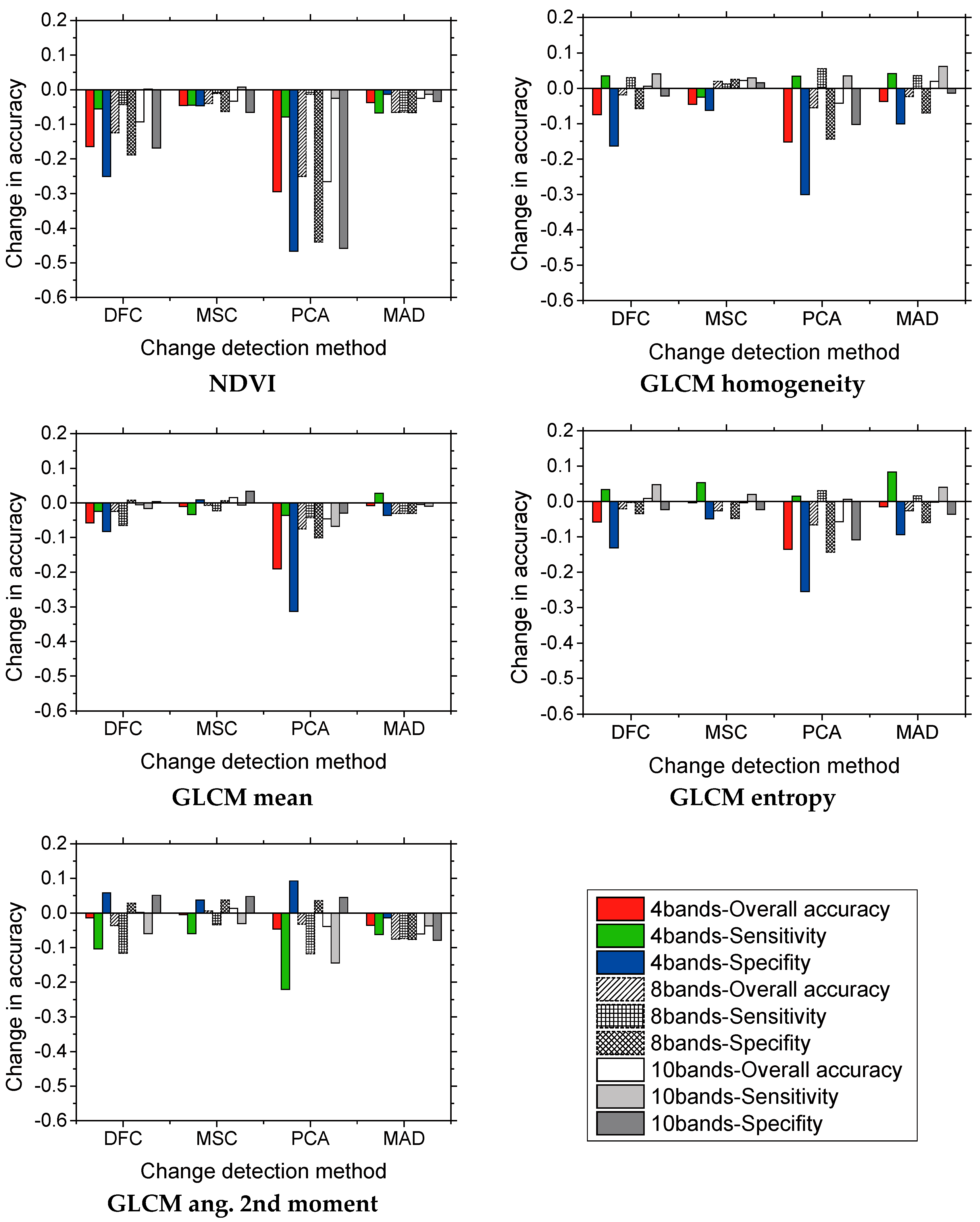
4.3. The Effect of Additional Parameters on Detection Accuracy

The results of further investigations into the effect of including additional textural and NDVI information in each segmentation strategy using these four methods (at a fixed confidence level of 0.9 and a segmentation scale of 140) are shown in Figure 7 and Figure 8. The results indicate that adding individual object-level textural or NDVI information did not generally lead to better accuracy in the different method and segmentation strategy combinations than using only spectral parameters. On the contrary, the three measures of accuracy frequently yielded worse results with the additional information than with spectral parameters alone; the magnitudes of changes with the additional information were also inconsistent between the different features, change detection methods, and segmentation strategies. Improvements in accuracy with the addition of textural or NDVI information only occurred in a few cases, and these occasional improvements amounted to no more than 5%, whereas reductions in accuracy were common and were up to 50%. In most cases, PCA was the method most sensitive to the extra textural and NDVI information, followed by MAD; the DFC and MSC methods were both influenced to a similar degree.

5. Discussion

This study has evaluated the effects of segmentation strategy, scale, feature space and unsupervised method for object-based change detection within an urban area (Changzhou, China). The validation procedure has demonstrated that the change detection accuracies were impacted by the uncertainty of parameters and methods in OBCD, where the segmented object was considered as the change detection unit instead of pixel.

5.1. The Utility of OBCD and Segmentation Scales

Our results demonstrate the utility of an object-based change detection and confirm the importance of the selected segmentation scale in such an approach. The highest accuracies in most cases did not occur at the fine segmentation scales (close to pixel size) but in the coarser segmentation scale range from 100 to 200. The lowest accuracies were observed at segmentation scales close to the pixel size. For Study site 1, the accuracy of the change map at a scale of 100 (88.2%) was better than that at a scale of 20 (83.02%) (Figure 9e) when using the MAD method. We assumed that this was related to “sliver objects”, i.e., spurious polygons generated within an area that is easily identified as having changed due to slightly different delineations of the same entity [47], which may occur because of difficulties in achieving high accuracy co-registration for high-resolution imagery and also because quite diverse information can be obtained on the same object from bi-temporal images due to off-nadir viewing angles [8]. These phenomena are more common at fine segmentation scales (Figure 9c), while the merging of objects at coarse segmentation scales allows these effects to be more or less eliminated by smoothing the local object-level variability (Figure 9b), although some sub-objects are likely to remain undetected. In other words, object-based methods are capable of providing improved performance over pixel-based methods for change detection in high-resolution imagery [9], since more slivers and gaps are likely to occur at pixel level.

5.2. Effects of Different Segmentation Strategies

We were somewhat surprised that, in this study, single-date segmentation using the four bands strategy generally had a higher sensitivity than two-date segmentation strategies, although it was assumed that changes on a sub-object scale might remain undetectable in single-date segmentation using the same confidence level [18]. We attributed the improved sensitivity to the integrality of changed objects in the single-date segmentation strategy, whereas two-date segmentation produced more fragmented patches. For instance, a change from fragmented bare land to a building could be more easily detected using single-date segmentation than using two-date segmentation. Unfortunately, the improvement in overall accuracy seems to be largely driven by the specificity, with there being a smaller probability of being wrong due to the reduced number of objects considered to have changed [20]. Two-date segmentations are therefore suggested to contribute more to the unsupervised change detection method than expected because the specificity benefitted more from the two-date segmentation strategies.

5.3. Effects of Different Unsupervised Change Detection Methods

Since the same detection technique (based on a chi-square statistic) was used for four input differencing vectors, the measures of accuracy were strongly related to the threshold determined by the confidence level and the degree of freedom. None of the four methods were found to have a dominant advantage over the others since the same accuracy level could be achieved by considering different confidence levels, and it was noted that threshold selection was critical for all of these methods. However, the good performance of MAD with the same parameters can be attributed to its use of the uncorrelated variables from canonical correlation analysis [37]. For PCA, the largest change in magnitude was commonly observed when additional textural and/or NDVI information was used to calculate the principle components. We assumed that this was related to the fixed three degrees of freedom because PCA always lost some information more or less with the first three components. Subsequently, it can be concluded that MAD seems to be a superior unsupervised change detection method for an OBCD scheme.

5.4. The Lack of Accuracy Improvement with Additional Features

It should be noted that, in most cases, the unsupervised change detection methods considered in this study were unable to benefit from the investigated additional features other than spectral parameters. The lack of improvement in accuracy with the inclusion of additional features may be attributable to the low capability of these change detection methods for dealing with multi-dimensional data [18]. However, the extra features certainly provide more information that should improve the accuracy of change detection in remote sensing imagery (e.g., for NDVI see Ward et al. [48] and for textural features see Im et al. [49], even though different methods were used). An improvement in overall accuracy with additional information on entropy was observed by Yang et al. [13] using an object-based method, although adding NDVI had a detrimental effect on the accuracy. Further improvements in OBCD would therefore require an improved change detection method that was able to take advantage of additional information such as textural information.

6. Conclusions

This paper presents a systematic analysis of object-based change detection to explore the effects that segmentation strategies, segmentation scales, feature space, and the choice of four unsupervised change detection methods have on the accuracy of change detection. We found that object-based methods at medium segmentation scales yielded a far higher level of overall accuracy than the same methods at fine segmentation scales close to the pixel size, with the segmentation scale that yielded maximum accuracy varying with the change detection method. The use of two-date segmentation for object generation was found to improve change detection with the tested methods. Choosing the optimal threshold appeared to improve the accuracy of each method, but MAD was still found to be superior to the other tested methods, under equivalent conditions. The inclusion of additional textural and NDVI information failed to improve the accuracies of these four unsupervised change detection methods. Future work will need to be directed towards the development of improved change detection methods that are able to take advantage of textural and other information derived from the segmented objects.