Article

Voxel-Based Spatial Filtering Method for Canopy Height Retrieval from Airborne Single-Photon Lidar

1
Department of Geographical Sciences, University of Maryland, College Park, MD 20742, USA
2
Sigma Space Corporation, 4600 Forbes Blvd, Lanham, MD 20706, USA
*
Author to whom correspondence should be addressed.
Submission received: 27 June 2016 / Revised: 6 September 2016 / Accepted: 12 September 2016 / Published: 19 September 2016
(This article belongs to the Special Issue Airborne Laser Scanning)

Abstract

:
Airborne single-photon lidar (SPL) is a new technology that holds considerable potential for forest structure and carbon monitoring at large spatial scales because it acquires 3D measurements of vegetation faster and more efficiently than conventional lidar instruments. However, SPL instruments use green wavelength (532 nm) lasers, which are sensitive to background solar noise, and therefore SPL point clouds require more elaborate noise filtering than other lidar instruments to determine canopy heights, particularly in daytime acquisitions. Histogram-based aggregation is a commonly used approach for removing noise from photon counting lidar data, but it reduces the resolution of the dataset. Here we present an alternate voxel-based spatial filtering method that filters noise points efficiently while largely preserving the spatial integrity of SPL data. We develop and test our algorithms on an experimental SPL dataset acquired over Garrett County in Maryland, USA. We then compare canopy attributes retrieved using our new algorithm with those obtained from the conventional histogram binning approach. Our results show that canopy heights derived using the new algorithm have a strong agreement with field-measured heights (r2 = 0.69, bias = 0.42 m, RMSE = 4.85 m) and discrete return lidar heights (r2 = 0.94, bias = 1.07 m, RMSE = 2.42 m). Results are consistently better than height accuracies from the histogram method (field data: r2 = 0.59, bias = 0.00 m, RMSE = 6.25 m; DRL: r2 = 0.78, bias = −0.06 m and RMSE = 4.88 m). Furthermore, we find that the spatial-filtering method retains fine-scale canopy structure detail and has lower errors over steep slopes. We therefore believe that automated spatial filtering algorithms such as the one presented here can support large-scale, canopy structure mapping from airborne SPL data.

Graphical Abstract

1. Introduction

Single photon lidar (SPL) is a new technology for rapid three-dimensional mapping of terrain and forest structure over large areas at high resolution [1]. SPL requires only one detected photon at each ranging measurement, instead of hundreds in the case of conventional sensors [2,3]. It therefore allows enhanced 3D mapping with greater coverage, spatial resolution, and photon density, and reduced acquisition time. Despite these advantages, SPL data includes more solar background noise than conventional near-infrared lidar instruments because of its use of green wavelength lidar and high photon detecting sensitivity [4,5,6]. This complicates the retrieval of terrain and canopy structural information from SPL data. Algorithms for efficiently handling noise in photon counting data are only beginning to be developed [7,8,9]. Existing methods largely rely on detecting maximum canopy height through histogram-based filtering algorithms [4,8,10,11]. This is achieved by aggregating point clouds into pseudo-waveforms at coarse spatial and vertical resolutions. Traditional waveform processing algorithms are then applied to the waveforms to derive canopy structure metrics including canopy height and cover. Although these methods have proven effective in filtering solar noise [4,8,10,11], the 3D structural detail in the dataset is reduced. It means that these methods forfeit a key advantage of SPL data over other systems—the ability to provide fine scale topographic and structural details. Applying histogram based filtering methods to SPL data would therefore drastically reduce its usefulness for applications such as high-quality topographic mapping [12], individual tree-level classification [13] and high resolution carbon monitoring [14,15]. Furthermore, histogram based filtering methods could potentially have errors over complex terrain because of the mixing between ground/canopy signals and noise points. To overcome these hurdles, we develop a spatial filtering algorithm that filters noise points using a variable 3D pixel (voxel) binning approach while retaining the spatial and vertical fidelity of the dataset.
We first describe data collection and the development of the spatial filtering algorithm. Next, we test it with airborne SPL data collected over Garrett County in Maryland [16] using an experimental High-Resolution Quantum Lidar System (HRQLS) instrument. We then compare canopy height metrics derived from SPL data, using both our algorithm and the conventional histogram filtering method, with the reference dataset collected from field campaigns and discrete return lidar (DRL). Lastly, we discuss the strengths and weaknesses of the two approaches and their applicability to large-scale forest mapping.

2. Materials and Methods
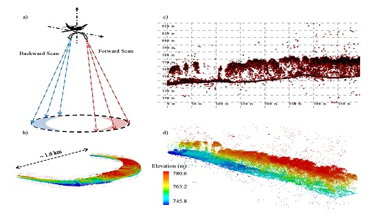
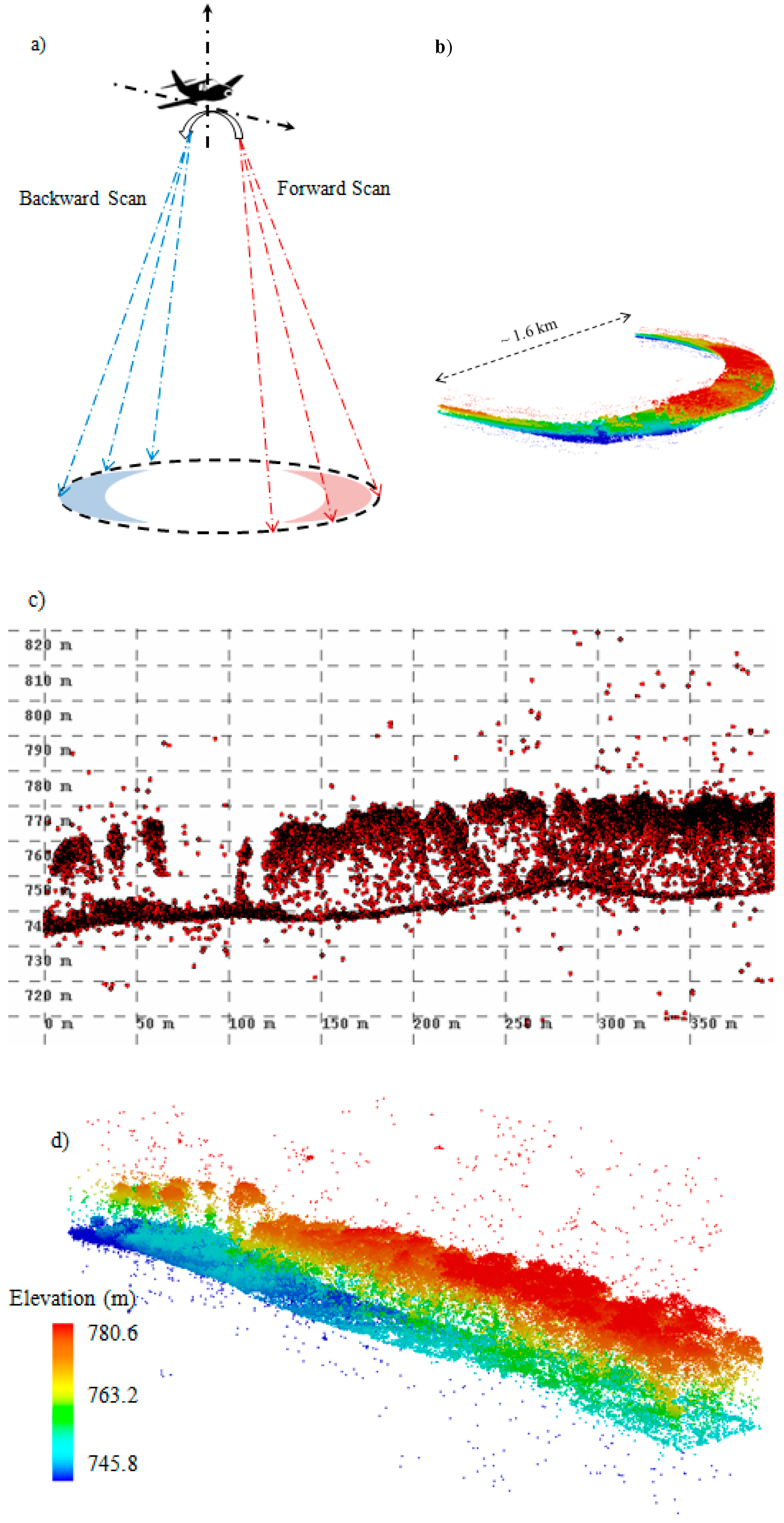
2.1. HRQLS

The High-Resolution Quantum Lidar System (HRQLS) is a moderate altitude SPL instrument with 10 × 10 laser beamlets and an operating wavelength of 532 nm. It is equipped with a dual wedge scanner allowing a full conical observing angle from 0° to 40°. HRQLS was flown over Garrett county of Maryland, USA in early September of 2013 to support a NASA Carbon Monitoring System (CMS) project over the state of Maryland [15,16]. The flight survey required less than 12 h to cover the entire county (~1700 km2) with 50% overlap of flight lines. At a nominal above ground level (AGL) of 2.3 km, HRQLS produced a swath of 1.62 km and a target spot of 5 × 5 m array on the ground, resulting in a ground-pixel dimension of 0.5 m and a mean point density of 12 per m2 per conical scan (including both signal and noise, see Figure 1). More details about the HRQLS data can be found in [2].

2.2. Reference Data

Field measurements were collected during the summer of 2013 with a main survey focus on aboveground biomass estimates [15]. Field plots (fixed and variable radius) were selected using a stratified random sampling based on distributions of land cover type and canopy height. We measured diameter at breast height (DBH) of each individual tree to estimate plot level biomass. Field heights were recorded using a vertex hypsometer with sonic transponder attached to dbh of the largest tree within 71-forested plots. Non-forested plots were excluded because no field height measurement was recorded.
Discrete return lidar (DRL) data were collected by USGS over Garrett County in 2005 as part of their floodplain mapping efforts. These data were collected in leaf-off season, and the point clouds included first returns only with an average density of 1 per m2. Both maximum canopy height (p100) and mean plot-level slope were extracted over the 71 field plots. Studies have suggested that those leaf-off lidar data sets can largely provide reliable canopy height measurements with accuracy similar to leaf-on data [17,18]. The comparison between leaf-off DRL and leaf-on field data produced r2 = 0.63, bias = −0.26 m and RMSE = 5.37 m despite ~10 year difference [1]. These data sets might not be an optimal reference for assessing SPL-derived canopy heights at highest possible precession, but they could still serve as a benchmark for comparison when used together.

2.3. HRQLS Data Processing

2.3.1. Preprocessing

HRQLS data was collected and pre-processed using proprietary software by Sigma Space Corporation (Lanham, MD, USA) [2]. A level 1 filter was applied to filter noise from the atmospheric column extending up to flight AGL. The filter searched the entire ranging measurements using a 30 m histogram of photon density and identified the peak interval as ground surface range. The level 1 filtered SPL dataset was then produced using points extracted within one interval above and below the peak to include signals from low terrain surfaces and tall canopies. It was essentially a 90 m vertical range subset of raw HRQLS, and reduced the mean point density to about 22 per m2. The Level 1 filter removed more than 90% of the solar noise from the entire vertical column [2] but considerable noise points remained in the 90 m vertical range subset and required further filtering.

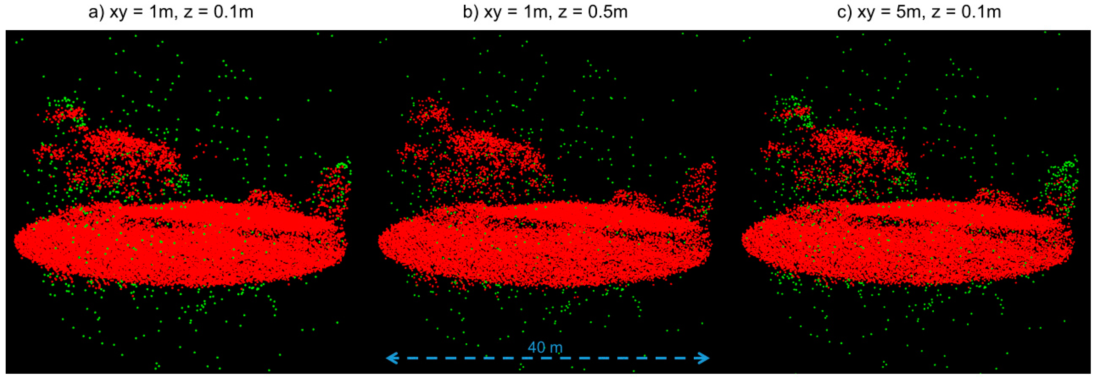
2.3.2. The Voxel-Based Spatial Filtering Method

A point density based spatial filter was developed to filter noise from the Level 1 SPL dataset (Figure 2). This filter identified noise points by searching isolated points in 3D space based on following assumptions: First, SPL points were treated as either signal or noise, and the majority of noise points were randomly distributed in 3D space. Second, noise level over a given area of interest was dependent on the incident laser energy indicated by the total amount of point clouds. For example, an overlap of two flight lines would double the amount of both signal and noise. Third, the density of signal point was significantly higher within the canopy-terrain layer than in the atmosphere. Last, all points in a voxel would be classified as signals if their total number exceeding a certain threshold. This voxel-based approach was similar to methods previously applied in processing airborne or terrestrial lidar data [19,20,21]. A detailed implementation of the algorithm was described as follows:
  • Calculating the maximum-noise-level threshold as the mean volume point density (points per m3) of the Level 1 SPL dataset at each 30 m × 30 m horizontal grid;
  • Splitting the area of interest into 3D cells at a given size;
  • Counting the number of points in each cell and its surrounding cells (a total of 27 cells);
  • Labeling the points as noise if the number was less than the pre-calculated noise threshold multiplied by the volume of 27 cells.
We determined the optimal filter by experimenting with different voxel sizes. In each experimental run, canopy heights were retrieved after noise filtering with different 3D voxel sizes and then compared with reference data while keeping other conditions the same. A 3 × 3 × 0.2 m voxel resulted in the lowest bias value of mean canopy height and was determined to be the optimal filter in this study. The optimal filter was applied to the Garrett county SPL dataset to produce a relatively ‘noise-free’ dataset for further analyses [1]. We then classified the point clouds into ground and canopy and calculated canopy height percentiles over the field plots. Ground points were identified based on a progressive Triangular Irregular Network (TIN) densification method by iteratively selecting points within lowest elevation values [22]. Canopy height percentile here was defined as the height below which a specified percentage of total point clouds were located, and it was calculated from the unclassified remaining points above the ground reference. For this study, canopy height percentiles were calculated at every 5 percentage increment starting from ground to canopy top (e.g., p05, p10, ..., p100), and at every 1 percentage increment starting from p96 to p100. The entire procedure from de-noising to canopy metric calculations was automated by customizing scripts from (lasnoise, lasground and lascanopy) the LAStools software [23].

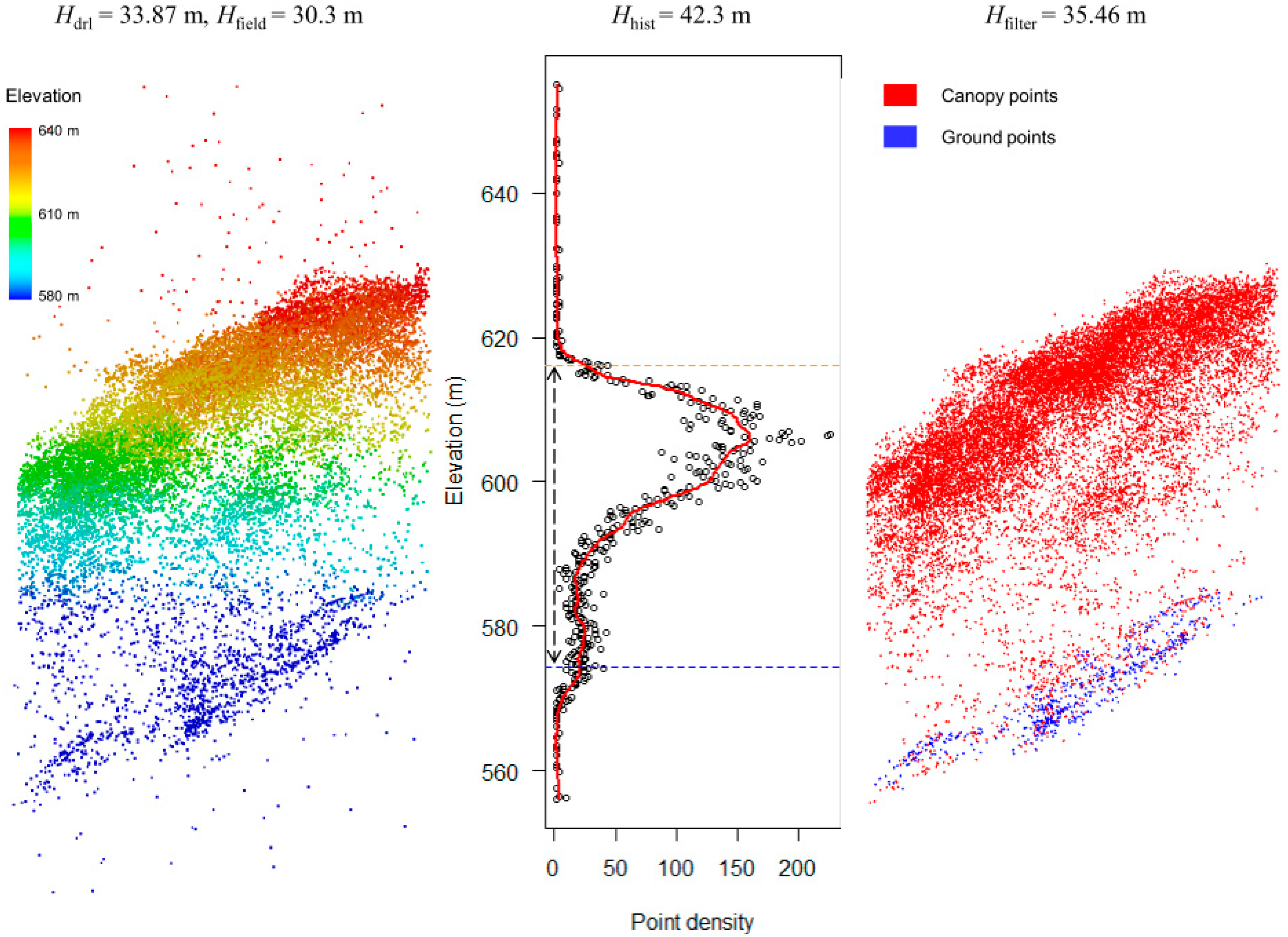
2.3.3. The Histogram Based Method

Next, we applied the histogram method to calculate canopy height from the level 1 dataset (Figure 2). The histogram method was a typical approach used to process photon counting lidar in many recent studies [4,8,10,11]. In this approach, photon-counting data were converted into pseudo-waveforms by aggregating lidar returns in user-defined elevation bins and footprint sizes. Canopy height metrics were then calculated from the pseudo-waveform using conventional waveform processing methods (e.g., identifying canopy top and ground elevation and height percentiles within each waveform). Here we did not apply any correction method to adjust a possible slope-induced error (e.g., usually requires DRL-derived slope map), because we aimed to compare their performances using information readily available from SPL only (the spatial-filtering vs. the histogram method).
In this study, we created SPL histograms over 71 field plots using a 0.15 m vertical resolution and a footprint radius of 15 m. The applied resolution and scale was identical to both field survey and previous studies [4,8,10,11]. We first normalized each histogram between 0 and 1 to compensate for spatial difference in photon density. We then subtracted the mean value from the normalized histogram and smoothed it using a Hann function with a window size of 8 (Hann function is a typical smoothing window method applied in signal processing) [24]. Bins with negative values in the smoothed histogram were identified as noise and were flattened to zero for further analysis. The subtraction and smoothing procedure separated signal ranges (ground and canopy) from noise ranges using the assumption that photons at ground and canopy range had a significantly higher density.
We then detected elevations of ground peak and canopy top using waveform lidar processing methods. Mean ground elevation was identified as the lowest mode of local maximum values in the smoothed histogram. Canopy top elevation was detected using a cut-off threshold value, calculated as the greater number between 0.01 and the maximum value within the highest 10 histogram bins. Finally, plot level canopy height was calculated as the difference between mean ground and canopy top elevations. In addition, we calculated canopy height percentiles by aggregating the histogram bins between ground and canopy top.

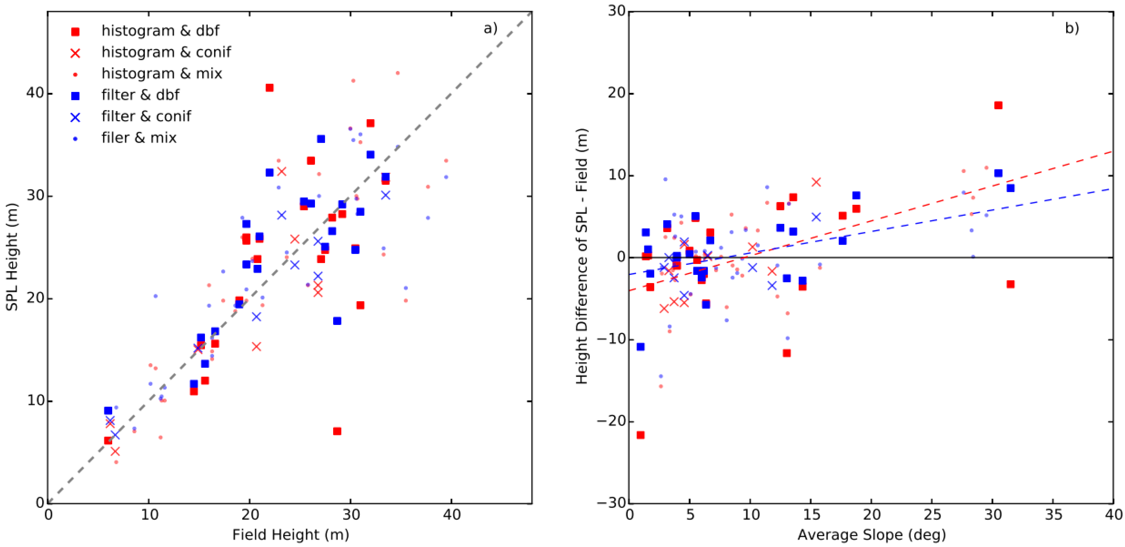
2.4. Canopy Height Comparison

We compared canopy heights calculated from the two methods using field measurements and discrete return lidar (DRL) as references. This was because of the lack of a ground reference for differentiating and validating noise/signal points. For both two methods above, we chose the p99 metric, rather than p100, to represent the true canopy height derived from SPL data. This was because p99 was a better indicator of canopy top height, particularly when anomalous laser returns may be present (e.g., birds or thin clouds for conventional lidar, and unfiltered noise points in this case) [25,26,27,28]. Comparisons were made using the following statistical variables: coefficient of determination (r2), bias (mean difference between SPL height and reference data) and root mean square error (RMSE). The height differences between SPL and reference data were analyzed as a function of the topographic slope using an ordinary least square (OLS) linear regression method. We also assessed potential impacts of using different voxels sizes on the performance of the spatial filtering method.

3. Results

Canopy height percentiles (p96 to p100) derived from the spatial-filtering method showed strong agreement with field and DRL data as demonstrated by the r2, bias, and RMSE values. Most of the height percentiles, except for the p100, achieved r2 > 0.7 in comparison with field measured canopy heights and r2 > 0.9 when compared with DRL derived heights (Table 1). The r2 between the 100th height percentile (i.e., p100) and reference heights was much lower than those between the other canopy height percentiles (p96~99) and reference data. Additionally, the p100 metric presented positive bias with values greater than ~3 m against the field height. Such high bias values were not observed in the other percentiles (p96~99), all of which presented consistently better agreements with reference data than p100. For example, the 98th percentile height showed the highest agreement with field data r2 = 0.70, bias = −0.12 m and RMSE = 4.77 m, while p97 had the lowest bias of 0.07 when compared with DRL heights.
Correspondingly, canopy height percentiles derived from the histogram method also achieved good agreements with the reference data. All height percentiles (including p100) showed highly similar results in their comparisons with reference data (r2 = 0.60 and RMSE ≈ 6.3 m for field heights, and r2 = 0.78 and RMSE ≈ 4.9 m for DRL respectively). The r2 values were 10%–15% lower than those from the filtering method, and the RMSE values were almost doubled in comparisons with DRL (Table 1). Unlike the filtering method, p100 values derived using the histogram approach had a smaller bias (~0.7 m) than the reference data and other height percentiles (p96~p99).
Canopy heights (the p99) derived from the spatial-filtering method (Hfilter) achieved consistently better agreements with reference data than those derived from the histogram method (Hhist) (Figure 3 and Figure 4, and Table 1). We found no significant impact on height measurement error among different forest types (all p > 0.1 using Welch’s t-test). However, canopy height differences (ΔH) between Hhist and the reference data were positively correlated with the topographic slope based on the OLS linear regression analysis (red-dotted line in Figure 3b and Figure 4b). The relationship was ΔH = 0.43 × Slope − 4.05 with r2 = 0.28 (p < 0.01) when compared to field data, and ΔH = 0.21 × Slope − 1.88 with r2 = 0.11 (p < 0.01) for DRL comparisons. In contrast, Hfilter showed a mild correlation with slope in field height comparisons: ΔH = 0.26 × Slope − 2.07 with r2 = 0.18 (p < 0.01); and there was no significant effect of slope spotted on the height difference between DRL and the Hfilter (p = 0.77). To better illustrate the effects of slope, we analyzed the point cloud in one of the field plots as an example (Figure 5). This plot was located on a steep slope of approximately 30°, canopy height measured in the field was 30.3 m and that from DRL data was 33.87 m. We found no discernible topographical effect on characterizing canopy structure using the spatial-filtering method with a Hfilter value of 35.46 m. Instead, the slope had a pronounced effect on the Hhist derived from the histogram method, leading to a highly overestimated value of 42.3 m.
Even on low-slope plots, the spatial-filtering method outperformed the histogram method, as seen from our analysis after excluding the plots of slope greater than 10°. Accuracies of the Hfilter did not change drastically, with r2 = 0.74, bias = −0.65 m and RMSE = 4.48 m against field heights and r2 = 0.95, bias = 0.79 m and RMSE = 1.95 m against DRL heights. The agreement between Hhist and DRL heights had a very slight improvement with r2 = 0.79, bias = −1.22 m and RMSE = 4.43 m, whereas the comparison between Hhist and field heights was greatly improved with r2 = 0.68, bias = −1.79 m and RMSE = 5.37 m.
The use of different voxel sizes in the spatial-filtering method had no pronounced impact on height retrieval performance at the plot level (Table 2). Comparison results with field measurements were similar among all voxel sizes except for the ultra-fine ones (e.g., a 1 × 1 × 0.1 m voxel). However, it may affect retrieval results at the individual tree level (Figure 6). Note that the vertical size of a voxel is not equivalent to vertical resolution, because voxels were only applied to remove noise photons (not for height extraction), and the remaining signal photons still have a continuous spatial distribution with a varying vertical distance (can be narrower or wider than the vertical voxel size [20].

4. Discussion

There is considerable interest in developing effective algorithms to obtain accurate canopy height measurements from daytime SPL data. This is important yet challenging for automated mapping over large areas because of the presence of solar noise [6]. The spatial filtering method developed in this study overcomes some of the drawbacks of conventional histogram binning [4,8,10,11], offering an alternative for processing large scale airborne SPL datasets.
Comparisons between SPL-derived canopy heights and reference data suggested that the two methods were able to derive canopy height data with reasonable accuracy. Both methods achieved good agreements with most r2 values greater than 0.6 and RMSE values less than 6 m. No significant bias was found either (<1 m). Our comparisons further indicated that the new method developed in this study could be more effective than histogram based methods, particularly for high point density SPL data, for several reasons:
First, the spatial-filtering method resulted in consistently better canopy height accuracies (higher r2, lower RMSE and low bias) than the histogram method as noted in comparisons with field and DRL data. The primary reason for this was that the spatial filtering method identified and filtered noise on an individual point basis, while the histogram-based method did not identify noise, per se, but rather eliminated it by identifying the highest mode at the canopy top and first mode at the bottom of the waveform. Because of this, it was expected to have errors over steep terrain where the ground was difficult to identify in the waveform. Second, canopy heights derived from the spatial-filtering method were only slightly impacted by the slope, a major contributor to errors in canopy height measurements using waveform lidar. Steep topography was known to affect ground detection and led to overestimated canopy heights [29,30,31]. It can also lead to an underestimation when having a higher noise threshold for a given waveform [32]. Potential correction methods (e.g., slope estimates from high-resolution DEM or waveform leading and trailing extent metrics) may help improve the waveform-based processing techniques [30]; however, their performance would largely depend on the availability of high-quality topography maps that were mostly derived from DRL. Such maps or robust correction approaches are not available nationally or globally. We noted that comparisons between Hfilter and field data were slightly affected by slope but believe it was more likely because of slope-induced errors in field height measurements (i.e., vertex method could be less accurate with large viewing angle) rather than in the spatial-filtering method. This was further confirmed in height comparisons between Hfilter and DRL. Comparisons with DRL proved that SPL heights derived using the spatial filtering method were clearly not affected by slope (Figure 4 and Figure 5). This could be because there was no aggregation in the spatial-filtering method and therefore fine-scale terrain variability did not affect it as strongly as in the case of the histogram approach. Third, the spatial filtering method did not transform the point cloud and retained its original 3D structure for downstream point cloud analyses, similar to conventional DRL data. This was critical in fine-scale analysis, such as crown delineation and individual tree identification [13,33], which may not be possible after histogram based filtering. This is because the transforming process of photon point clouds can lead to substantial loss of detailed spatial information (e.g., small scale topography variation), which cannot be retrieved back regardless of any further data processing method applied (e.g., the histogram method here). It also allowed fast batch process and direct visualization with no further requirement for format transformation (all files were stored in ASPRS las 1.2 format).
Interestingly, the histogram method was better at identifying canopy top, especially over low-slope plots, while the spatial-filtering method had errors (as noted from the lower accuracies of p100 heights). This was probably because canopies were more clustered and resulted in a strong peak in the pseudo-waveform at plot level. On the other hand, clustering at the canopy–atmosphere boundary made it difficult to separate signal from noise in the spatial-filtering method and even a few wrongly identified noise points could lead to large errors in the 100th percentile height. This was because the spatial filtering method was designed to remove noise at voxel level which had a higher spatial variation of photon density than the plot level. When the signal photon density was extremely low and had a similar level to the noise (e.g., from individual small tree), either a coarse horizontal resolution voxel or an extra-fine resolution one might fail to identify part of the crown (e.g., Figure 6). Overcoming this problem would require more research and improvements in the algorithm, but an effective and widely used solution was to use lower (p99 or p98) heights to represent canopy top and moderate voxel size as we did in this study [25,26,27,28].
Ultimately, the choice of processing method depends on the point density, quality, and extent of SPL data, particularly when SPL technology is still in the experimental stage. The histogram method is useful for a rapid analysis with moderate accuracy but will result in loss of spatial resolution and integrity. It can be mostly aimed at process datasets with low photon density (e.g., ICESat-2), which requires aggregation of points over transects to determine the profile of the canopy surface and the underlying topography. For applications involving airborne SPL, the spatial-filtering method is clearly a better choice. It can largely retain the 3D details with a much higher measurement accuracy, and is thus extremely valuable in fine-scale analysis. As an example, this method has been successfully implemented over the entire county of Garrett in Maryland, demonstrating its usefulness for large-scale terrain and canopy structure mapping [1]. However, this method may not be fully applicable to a dataset with extremely low point density because it violates the basic assumptions in the spatial-filtering method (see Section 2.3.2). Future studies would explore improvements in the density-dependent algorithm, particularly at the canopy-atmosphere boundary and over highly reflective urban targets. It would allow the process of ever-increasing SPL datasets from different platforms, and can extract canopy structure information efficiently over broad geographical areas.
When fully developed, the coupling of low acquisition cost and high processing efficiency together can revolutionize the use of airborne SPL in routinely forest monitoring. It will then serve as a relatively low cost and high efficient alternative to current airborne DRL systems, especially for large-area forest mapping [1]. For example, the area coverage rates of current HRQLS (~224 km2/h) [2] are more than three times higher than a DRL system, typically varying from about 50 to 80 km2/h in a bathymetry survey [34]. The density of lidar point clouds per scan is also much higher in a SPL data set (e.g., ~100 for HRQLS vs. < 5 for DRL). However, a direct cost-effective comparison between airborne SPL and DRL surveys is complicated because of both high variety in their platforms and sensor-related characteristics and the desired accuracy and density of lidar point clouds as well [35]. Considering the SPL system is still under fast development aiming to improve the quality and capacity of large-area mapping, we envision that there will be more large-scale high point density SPL data available in the near future [36,37]. These data sets, in together with existing high-quality DRL data [38,39], can allow large-scale analysis of ecosystem dynamics and carbon flux at high spatial resolution.

5. Conclusions

In this study, we have shown how high background solar noise in SPL can be efficiently filtered using voxel-based spatial filtering. The algorithm presented here can help derive standardized lidar products (e.g., canopy height model) under both high accuracy and great efficiency. This method could be applied to other photon-counting lidar acquisitions with high photon density as well. Further development of this can support fully automated processing of high point density SPL data over broad geographical areas, and facilitate routine monitoring of forest structure dynamics.

Acknowledgments

This study was funded by a NASA Carbon Monitoring System Grant (NNX12AN07G—Dubayah), a NASA Terrestrial Ecology Grant (NNX12AK07G—Dubayah) and a NASA Earth System Fellowship (NNX12AN43H—Dubayah/Tang). We also want to thank Martin Isenburg for his valuable feedback and technical support with the LAStools software package.

Author Contributions

H.T., A.S. and R.D. designed the experiments; P.D. and T.B. provided pre-processed and geo-referenced SPL data; H.T. and A.S. processed and analyzed the data; H.T., A.S. and R.D. wrote the paper with contributions from all other co-authors.

Conflicts of Interest

The authors declare no conflict of interest.

References

  1. Swatantran, A.; Tang, H.; Barrett, T.; DeCola, P.; Dubayah, R. Rapid, high-resolution forest structure and terrain mapping over large areas using single photon lidar. Sci. Rep. 2016, 6, 28277. [Google Scholar] [CrossRef] [PubMed]
  2. Degnan, J.J.; Field, C.T. Moderate to high altitude, single photon sensitive, 3D imaging lidars. SPIE Proc. 2014, 9114. [Google Scholar] [CrossRef]
  3. Degnan, J. Photon-counting multikilohertz microlaser altimeters for airborne and spaceborne topographic measurements. J. Geodyn. 2002, 34, 503–549. [Google Scholar] [CrossRef]
  4. Gwenzi, D.; Lefsky, M.A. Prospects of photon counting lidar for savanna ecosystem structural studies. Int. Arch. Photogramm. Remote Sens. Spat. Inf. Sci. 2014, 40, 141–147. [Google Scholar] [CrossRef]
  5. Rosette, J.; Field, C.; Nelson, R.; DeCola, P.; Cook, B. A new photon-counting lidar system for vegetation analysis. In Proceedings of the 11th International Conference on LiDAR Applications for Assessing Forest Ecosystems (SilviLaser 2011), Hobart, Australia, 16–19 October 2011.
  6. Glenn, N.F.; Neuenschwander, A.; Vierling, L.A.; Spaete, L.; Li, A.; Shinneman, D.J.; Pilliod, D.S.; Arkle, R.S.; McIlroy, S.K. Landsat 8 and ICESat-2: Performance and potential synergies for quantifying dryland ecosystem vegetation cover and biomass. Remote Sens. Environ. 2016. [Google Scholar] [CrossRef]
  7. Awadallah, M.S.; Abbott, A.L.; Thomas, V.A.; Wynne, R.H.; Nelson, R.F. Estimating forest canopy height and biophysical parameters using photon-counting laser altimetry. In Proceedings of the 13th International Conference on LiDAR Applications for Assessing Forest Ecosystems (SilviLaser 2013), Beijing, China, 9–11 October 2013.
  8. Herzfeld, U.C.; McDonald, B.W.; Wallin, B.F.; Neumann, T.A.; Markus, T.; Brenner, A.; Field, C. Algorithm for detection of ground and canopy cover in micropulse photon-counting lidar altimeter data in preparation for the ICESat-2 mission. IEEE Trans. Geosci. Remote Sens. 2014, 52, 2109–2125. [Google Scholar] [CrossRef]
  9. Magruder, L.A.; Wharton, M.E.; Stout, K.D.; Neuenschwander, A.L. Noise filtering techniques for photon-counting ladar data. SPIE Proc. 2012, 8379. [Google Scholar] [CrossRef]
  10. Moussavi, M.S.; Abdalati, W.; Scambos, T.; Neuenschwander, A. Applicability of an automatic surface detection approach to micro-pulse photon-counting lidar altimetry data: Implications for canopy height retrieval from future ICESat-2 data. Int. J. Remote Sens. 2014, 35, 5263–5279. [Google Scholar] [CrossRef]
  11. Montesano, P.M.; Rosette, J.; Sun, G.; North, P.; Nelson, R.F.; Dubayah, R.O.; Ranson, K.J.; Kharuk, V. The uncertainty of biomass estimates from modeled ICESat-2 returns across a boreal forest gradient. Remote Sens. Environ. 2015, 158, 95–109. [Google Scholar] [CrossRef]
  12. Lukas, V.; Eldridge, D.F.; Jason, A.L.; Saghy, D.L.; Steigerwald, P.R.; Stoker, J.M.; Sugarbaker, L.J.; Thunen, D.R. Status Report for the 3D Elevation Program, 2013–2014; U.S. Geological Survey: Reston, VA, USA, 2015; p. 17. [Google Scholar]
  13. O’Neil-Dunne, J.; MacFaden, S.; Royar, A. A versatile, production-oriented approach to high-resolution tree-canopy mapping in urban and suburban landscapes using geobia and data fusion. Remote Sens. 2014, 6, 12837–12865. [Google Scholar] [CrossRef]
  14. Goetz, S.; Dubayah, R. Advances in remote sensing technology and implications for measuring and monitoring forest carbon stocks and change. Carbon Manag. 2011, 2, 231–244. [Google Scholar] [CrossRef]
  15. Huang, W.; Swatantran, A.; Johnson, K.; Duncanson, L.; Tang, H.; O’Neil Dunne, J.; Hurtt, G.; Dubayah, R. Local discrepancies in continental scale biomass maps: A case study over forested and non-forested landscapes in Maryland, USA. Carbon Balance Manag. 2015, 10, 19. [Google Scholar] [CrossRef] [PubMed]
  16. Dubayah, R.; Swatantran, A.; Huang, W.; Duncanson, L.; Johnson, K.; Tang, H.; Dunne, J.O.; Hurtt, G. CMS: LiDAR-Derived Aboveground Biomass, Canopy Height and Cover for Maryland, 2011; ORNL Distributed Active Archive Center: Oak Ridge, TN, USA, 2016. [Google Scholar]
  17. Andersen, H.E.; McGaughey, R.J.; Reutebuch, S.E. Forest measurement and monitoring using high-resolution airborne lidar. In USDA Forest Service—General Technical Report PNW; USDA Forest Service: Washington, DC, USA, 2005; pp. 109–120. [Google Scholar]
  18. Wasser, L.; Day, R.; Chasmer, L.; Taylor, A. Influence of vegetation structure on lidar-derived canopy height and fractional cover in forested riparian buffers during leaf-off and leaf-on conditions. PLoS ONE 2013, 8, e54776. [Google Scholar] [CrossRef] [PubMed]
  19. Popescu, S.C.; Zhao, K. A voxel-based lidar method for estimating crown base height for deciduous and pine trees. Remote Sens. Environ. 2008, 112, 767–781. [Google Scholar] [CrossRef]
  20. Hancock, S.; Essery, R.; Reid, T.; Carle, J.; Baxter, R.; Rutter, N.; Huntley, B. Characterising forest gap fraction with terrestrial lidar and photography: An examination of relative limitations. Agric. For. Meteorol. 2014, 189, 105–114. [Google Scholar] [CrossRef] [Green Version]
  21. Cote, J.F.; Widlowski, J.L.; Fournier, R.A.; Verstraete, M.M. The structural and radiative consistency of three-dimensional tree reconstructions from terrestrial lidar. Remote Sens. Environ. 2009, 113, 1067–1081. [Google Scholar] [CrossRef]
  22. Axelsson, P. Dem generation from laser scanner data using adaptive tin models. Int. Arch. Photogramm. Remote Sens. 2000, 33, 111–118. [Google Scholar]
  23. Isenburg, M. LAStools—Efficient Lidar Processing Software (Version 140929); rapidlasso GmbH: Gilching, Germany, 2014. [Google Scholar]
  24. Harris, F.J. Use of windows for harmonic-analysis with discrete Fourier-transform. Proc. IEEE 1978, 66, 51–83. [Google Scholar] [CrossRef]
  25. D’Oliveira, M.V.N.; Reutebuch, S.E.; McGaughey, R.J.; Andersen, H.E. Estimating forest biomass and identifying low-intensity logging areas using airborne scanning lidar in Antimary State Forest, Acre State, western Brazilian Amazon. Remote Sens. Environ. 2012, 124, 479–491. [Google Scholar] [CrossRef]
  26. Riano, D.; Chuvieco, E.; Condes, S.; Gonzalez-Matesanz, J.; Ustin, S.L. Generation of crown bulk density for Pinus sylvestris L. from lidar. Remote Sens. Environ. 2004, 92, 345–352. [Google Scholar] [CrossRef]
  27. Frazer, G.W.; Wulder, M.A.; Niemann, K.O. Simulation and quantification of the fine-scale spatial pattern and heterogeneity of forest canopy structure: A lacunarity-based method designed for analysis of continuous canopy heights. For. Ecol. Manag. 2005, 214, 65–90. [Google Scholar] [CrossRef]
  28. Jaskierniak, D.; Lane, P.N.J.; Robinson, A.; Lucieer, A. Extracting lidar indices to characterise multilayered forest structure using mixture distribution functions. Remote Sens. Environ. 2011, 115, 573–585. [Google Scholar] [CrossRef]
  29. Duncanson, L.I.; Niemann, K.O.; Wulder, M.A. Estimating forest canopy height and terrain relief from glas waveform metrics. Remote Sens. Environ. 2010, 114, 138–154. [Google Scholar] [CrossRef]
  30. Lee, S.; Ni-Meister, W.; Yang, W.Z.; Chen, Q. Physically based vertical vegetation structure retrieval from ICESat data: Validation using LVIS in white mountain national forest, New Hampshire, USA. Remote Sens. Environ. 2011, 115, 2776–2785. [Google Scholar] [CrossRef]
  31. Miller, M.E.; Lefsky, M.; Pang, Y. Optimization of geoscience laser altimeter system waveform metrics to support vegetation measurements. Remote Sens. Environ. 2011, 115, 298–305. [Google Scholar] [CrossRef]
  32. Hancock, S.; Disney, M.; Muller, J.P.; Lewis, P.; Foster, M. A threshold insensitive method for locating the forest canopy top with waveform lidar. Remote Sens. Environ. 2011, 115, 3286–3297. [Google Scholar] [CrossRef]
  33. Duncanson, L.I.; Dubayah, R.O.; Cook, B.D.; Rosette, J.; Parker, G. The importance of spatial detail: Assessing the utility of individual crown information and scaling approaches for lidar-based biomass density estimation. Remote Sens. Environ. 2015, 168, 102–112. [Google Scholar] [CrossRef]
  34. Guenther, G.C. Airborne lidar bathymetry. In Digital Elevation Model Technologies and Applications: The DEM Users Manual, 2nd ed.; American Society for Photogrammertry and Remote Sensing: Bethesda, MD, USA, 2007; pp. 253–320. [Google Scholar]
  35. Wulder, M.A.; White, J.C.; Nelson, R.F.; Næsset, E.; Ørka, H.O.; Coops, N.C.; Hilker, T.; Bater, C.W.; Gobakken, T. Lidar sampling for large-area forest characterization: A review. Remote Sens. Environ. 2012, 121, 196–209. [Google Scholar] [CrossRef]
  36. Abdullah, Q.A. A star is born: The state of new lidar technologies. Photogramm. Eng. Remote Sens. 2016, 82, 307–312. [Google Scholar] [CrossRef]
  37. Li, Q.; Degnan, J.; Barrett, T.; Shan, J. First evaluation on single photon-sensitive lidar data. Photogramm. Eng. Remote Sens. 2016, 82, 455–463. [Google Scholar] [CrossRef]
  38. Asner, G.P.; Knapp, D.E.; Martin, R.E.; Tupayachi, R.; Anderson, C.B.; Mascaro, J.; Sinca, F.; Chadwick, K.D.; Higgins, M.; Farfan, W.; et al. Targeted carbon conservation at national scales with high-resolution monitoring. Proc. Natl. Acad. Sci. USA 2014, 111, E5016–E5022. [Google Scholar] [CrossRef] [PubMed]
  39. Cook, B.D.; Corp, L.A.; Nelson, R.F.; Middleton, E.M.; Morton, D.C.; McCorkel, J.T.; Masek, J.G.; Ranson, K.J.; Ly, V.; Montesano, P.M. NASA Goddard’s LiDAR, Hyperspectral and Thermal (G-LiHT) airborne imager. Remote Sens. 2013, 5, 4045–4066. [Google Scholar] [CrossRef]
Figure 1. An overview of single photon lidar (SPL) data acquired from the High-Resolution Quantum Lidar System (HRQLS): (a) The conical scanning mechanism of HRQLS with both forward and backward scans; (b) An example of point clouds acquired in an individual scan; (c) An example of cross sectional profile composited from multiple scans; (d) 3D point clouds including photons from canopy, terrain and solar noise.
Remotesensing 08 00771 g001
Figure 2. A flowchart of deriving canopy height from SPL data using two independent methods: the histogram based method and the spatial filtering method.
Remotesensing 08 00771 g002
Figure 3. (a) Comparisons between field heights and canopy heights (p99) derived from SPL data (using both histogram method and the spatial-filtering method); and (b) height differences between field data and SPL as a function of averaged slope value at each plot. For the histogram method ΔH = 0.43 × Slope − 4.05 with r2 = 0.28 (p < 0.01), and for the spatial-filtering method ΔH = 0.26 × Slope − 2.07 with r2 = 0.18 (p < 0.01). Symbols of different color and shape stand for different processing methods (red: histogram method, and blue: spatial-filtering method) over different types of forests (dbf: deciduous broadleaf forests, conif: coniferous forests, and mix: mixed forests).
Remotesensing 08 00771 g003
Figure 4. (a) Comparisons between canopy heights derived from discrete return lidar (DRL) and SPL data (using both histogram method and the spatial-filtering method); and (b) height differences between DRL and SPL as a function of averaged slope value at each plot. For the histogram method ΔH = 0.21 × Slope − 1.88 with r2 = 0.11 (p < 0.01). There was no significant relationship between ΔH and slope for the spatial-filtering method (p = 0.77). Same legend as Figure 3.
Remotesensing 08 00771 g004
Figure 5. A comparison example of plot-level canopy height products derived from SPL data using both histogram method and the spatial-filtering method. The plot is on a slope of about 30° with a DRL measured canopy height of 33.87 m and a field measured height of 30.3 m. The left part shows the raw level 1 HRQLS data over the plot with noises distributed both above and below the canopy-terrain layer. The center shows the pseudo-waveform generated from the histogram method, with identified canopy top (616.15 m), ground peak (574.35 m) and canopy height (42.3 m) in dash lines. The right part shows the noise-removal and point-classification results of HRQLS data using the spatial-filtering method. The ground points are in blue, and canopy points are in red with an estimated canopy height (p99) of 35.46 m.
Remotesensing 08 00771 g005
Figure 6. An illustrative example of the impact of different voxel sizes on noise removal at the individual tree level. The voxel sizes are expressed as combinations of different horizontal resolutions (xy, unit: m) and vertical resolutions (z, unit: m) in (ac). All the three voxels of different sizes can identify the majority of noise photons (green points) both above canopy and below ground. However, an extra-fine resolution voxel may fail to capture the top of individual trees (a), and an extra-coarse horizontal resolution voxel may miss the entire small tree in open space (c).
Remotesensing 08 00771 g006
Table 1. Comparisons between reference heights (from field data and discrete return lidar) and canopy height percentiles derived from the spatial-filtering method and the histogram method.
Spatial-Filtering SPL—Field Height SPL—DRL Height
Methodr2BiasRMSEr2BiasRMSE
p1000.542.886.990.833.775.46
p990.690.424.850.941.072.42
p980.70−0.124.770.940.492.28
p970.70−0.524.780.930.072.35
p960.70−0.884.820.92−0.312.52
Histogram SPL—Field Height SPL—DRL Height
Methodr2BiasRMSEr2BiasRMSE
p1000.590.776.410.780.685.05
p990.590.006.250.78−0.064.88
p980.60−0.526.240.78−0.554.89
p970.60−0.936.220.78−0.934.92
p960.60−1.316.250.78−1.294.99
Table 2. Performance of the spatial-filtering methods across different cell sizes when compared with field heights. The columns stand for different vertical resolutions (unit: m) and the rows are different horizontal resolutions (unit: m). Each cell describes the lowest RMSE achieved at a certain voxel size (optimal radius, r2, bias, RMSE).
z = 0.1z = 0.2z = 0.3z = 0.4
xy = 1(11, 0.67, −1.17, 5.09)(9, 0.74, −1.02, 4.44)(7, 0.75, −0.67, 4.44)(9, 0.73, 0.01, 4.50)
xy = 2(11, 0.71, −0.71, 4.65)(8, 0.77, −0.75, 4.17)(8, 0.76, −0.62, 4.22)(8, 0.75, −0.48, 4.37)
xy = 3(8, 0.77, −0.83, 4.22)(8, 0.76, −0.64, 4.22)(9, 0.75, −0.32, 4.28)(9, 0.75, −0.33, 4.35)
xy = 4(8, 0.76, −0.60, 4.23)(9, 0.75, −0.30, 4.35)(9, 0.75, −0.29, 4.30)(9, 0.75, −0.26, 4.30)
xy = 5(9, 0.74, −0.26, 4.41)(9, 0.74, −0.30, 4.44)(9, 0.75, −0.29, 4.38)(9, 0.74, −0.25, 4.39)

