
Sediment-Mass Accumulation Rate and Variability in the East China Sea Detected by GRACE


 , ,
, ,
Abstract
:
1. Background
2. Data and Method
2.1. GRACE Data
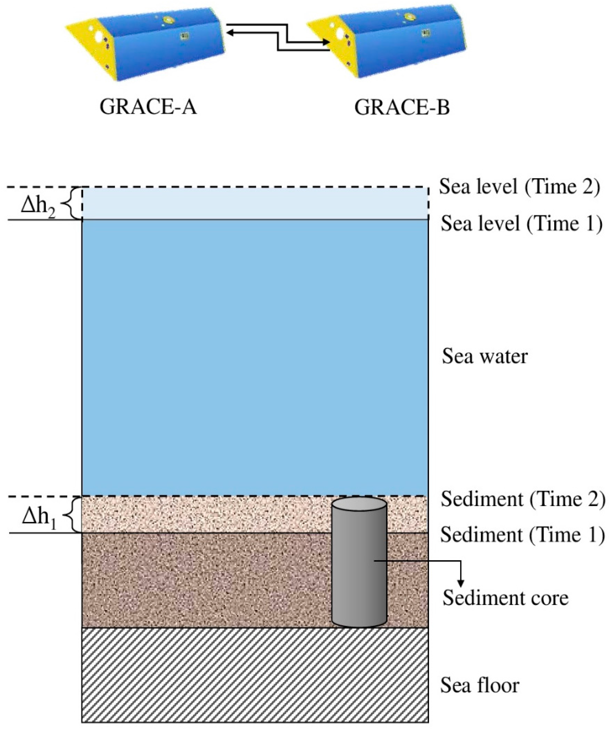
2.2. GRACE Determination of Mass Changes Associated with Sediment Deposition
2.3. Modelling Continental Hydrology Leakage Effect Using GLDAS
2.4. Mass Changes from GRACE and Due to Sea Level Change and Sediment Accumulation
3. Result
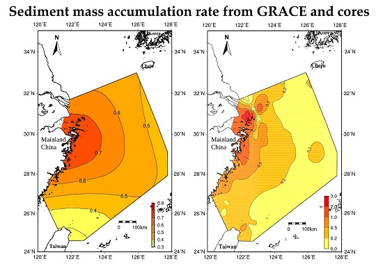
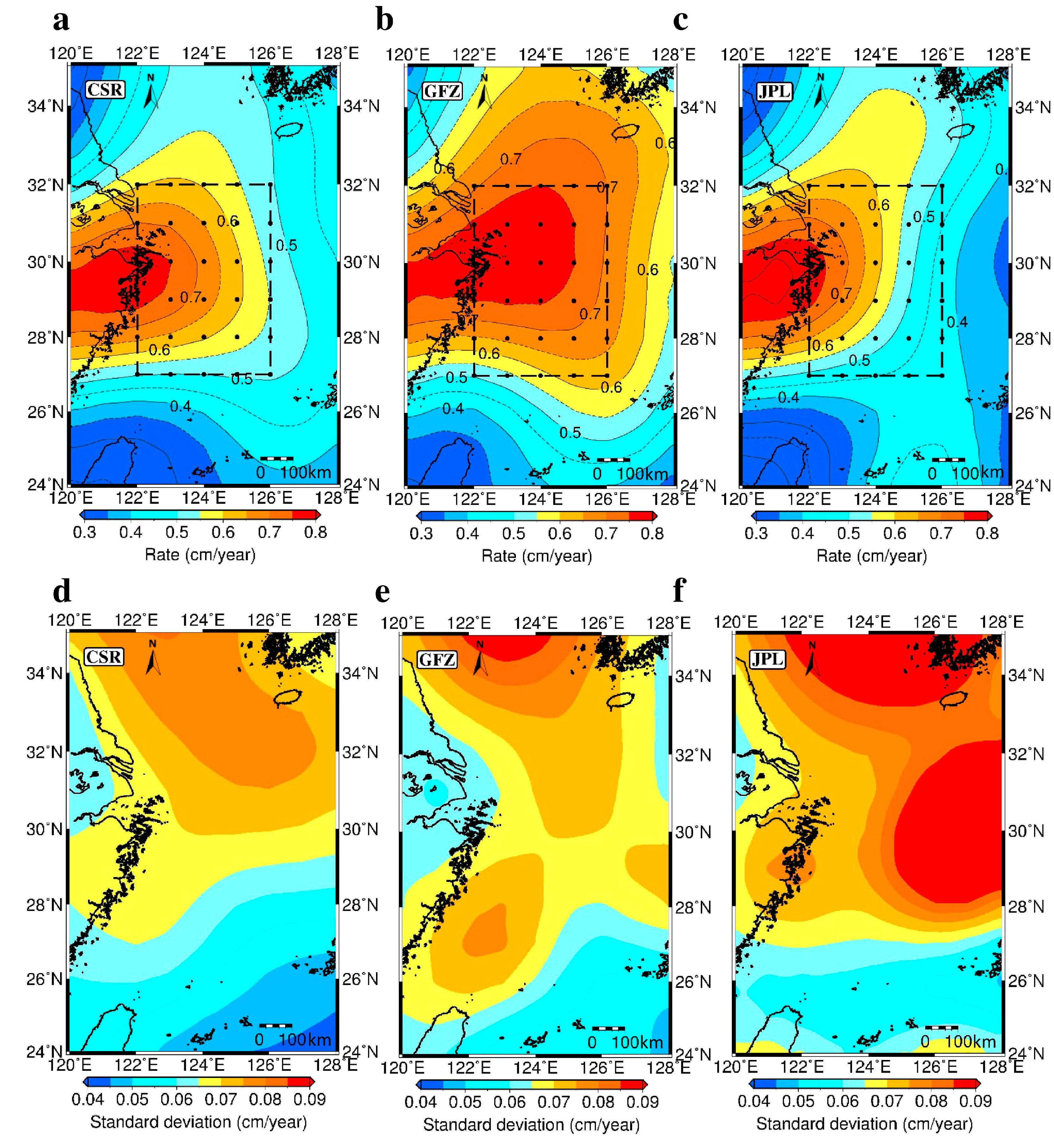
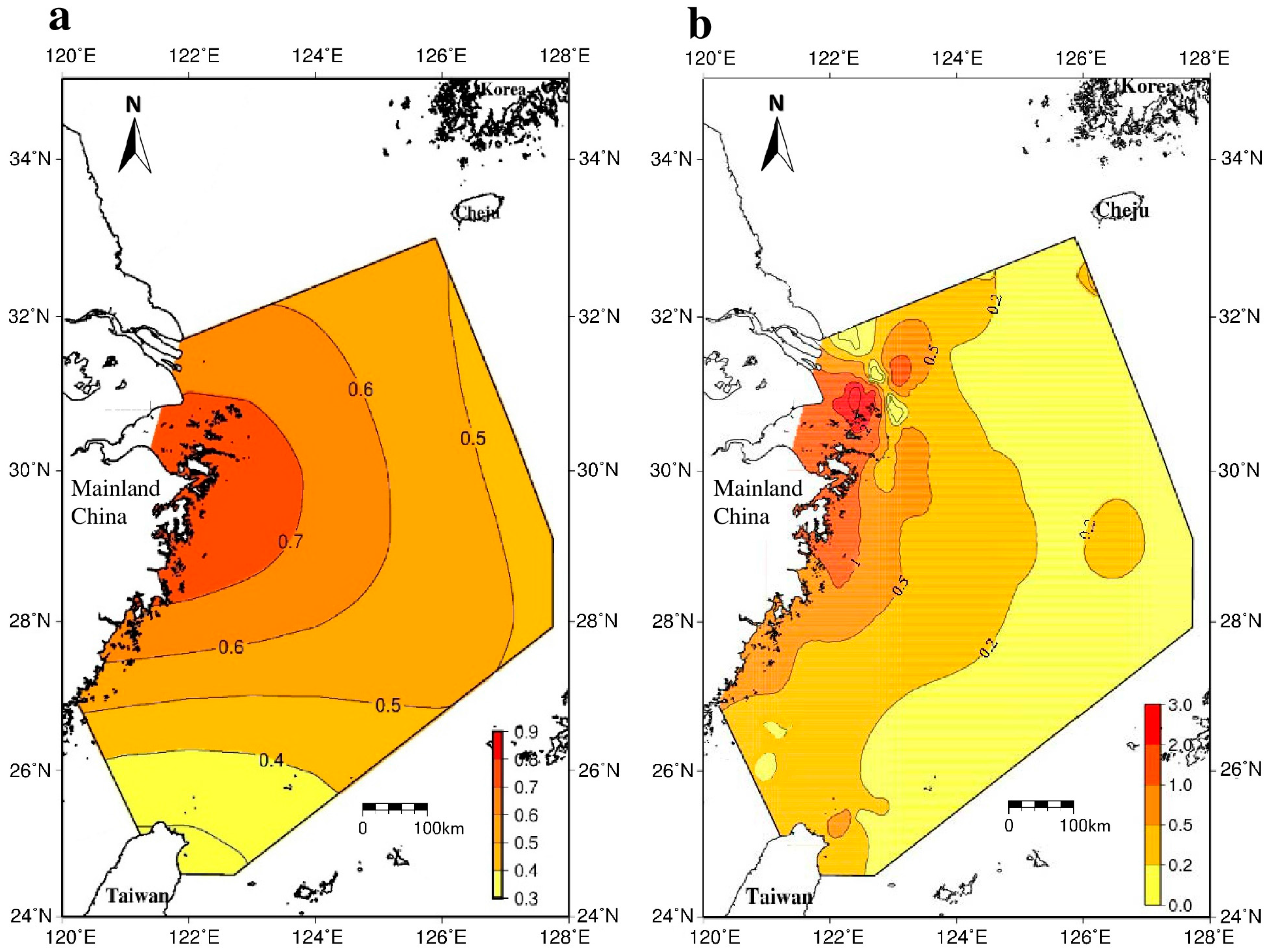
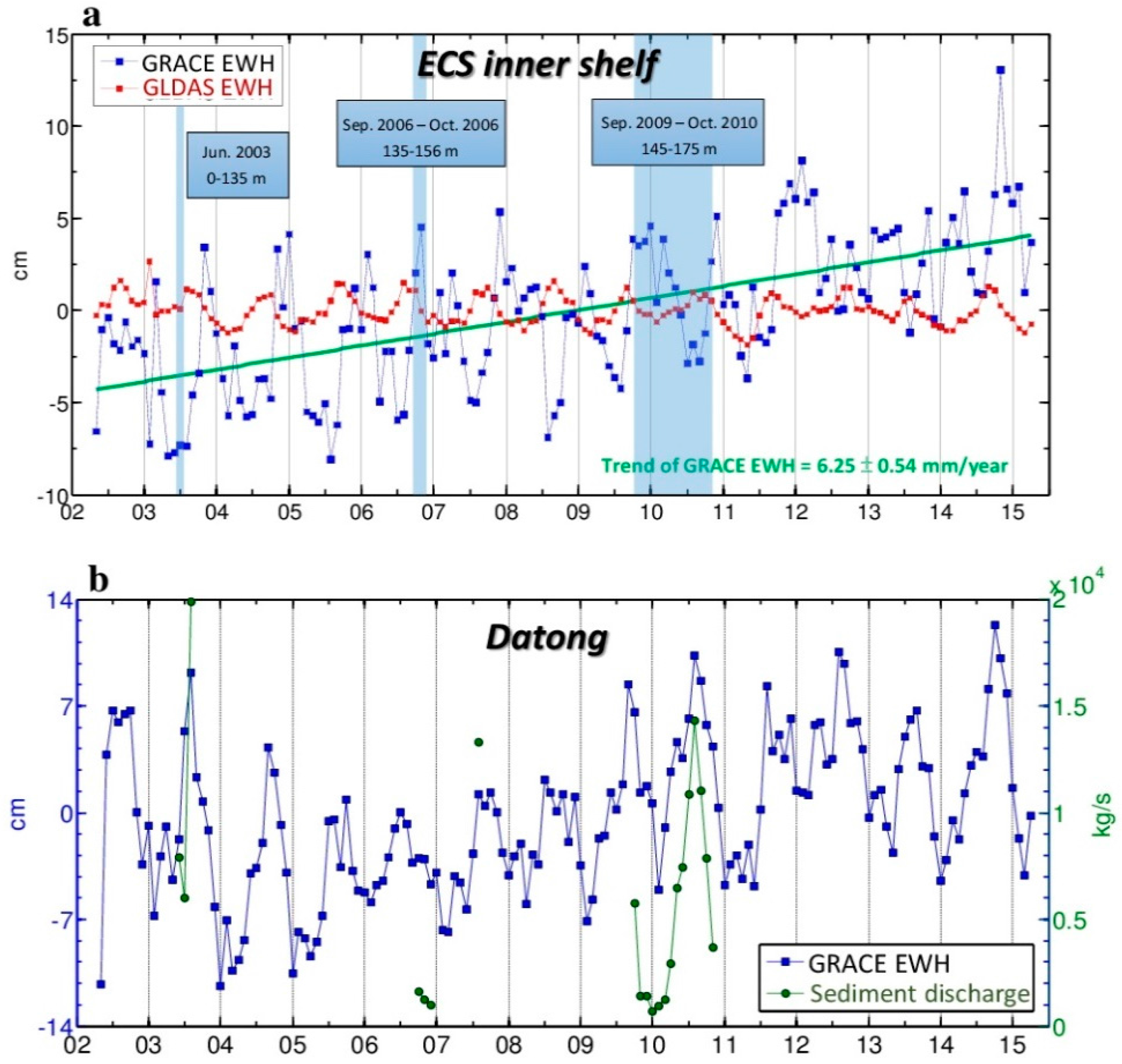
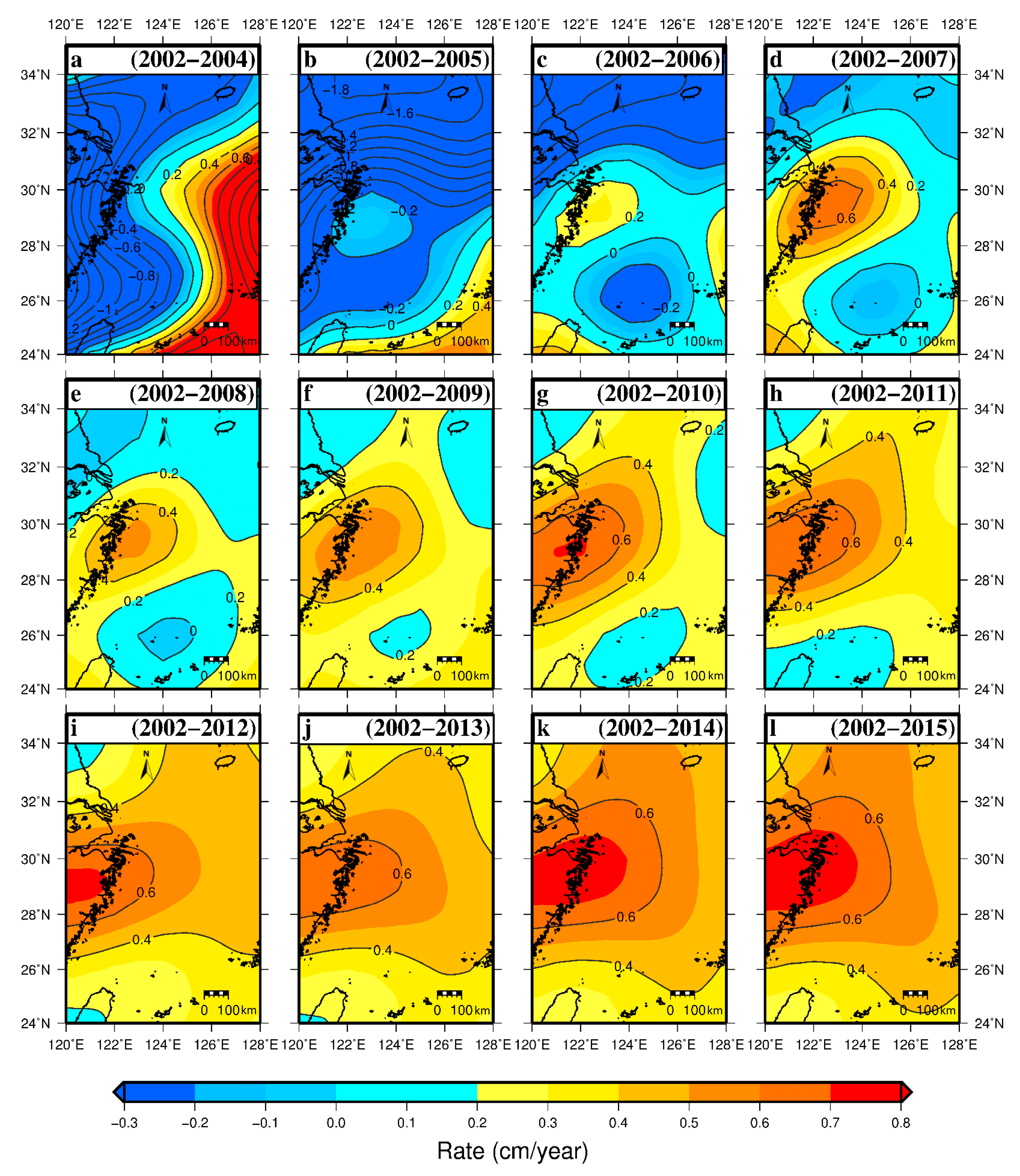
3.1. Sediment-Mass Accumulation: Rates from GRACE and Sediment-Core Measurements and the General Pattern
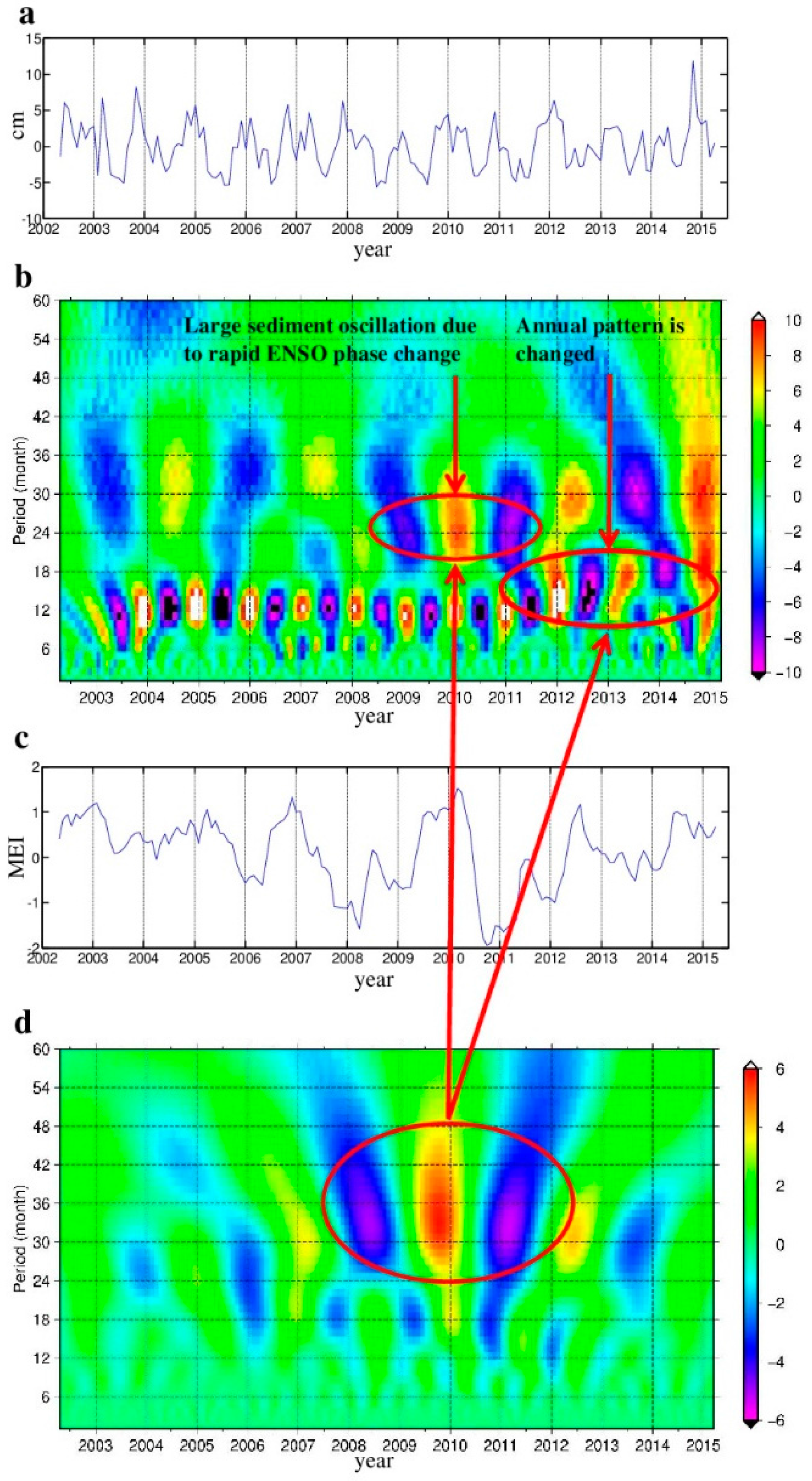
3.2. Variability of Sediment Mass in the ECS: From Semi-Annual to Inter-Annual Oscillations
3.3. Semi-Annual Oscillation (the Period Is Six Months)
3.4. Annual Oscillation (the Period Is 12 Months)
3.5. Quasi-Biennial Oscillation (the Period Is about Two Years)
3.6. Interannual Oscillation
3.7. Decadal Oscillation
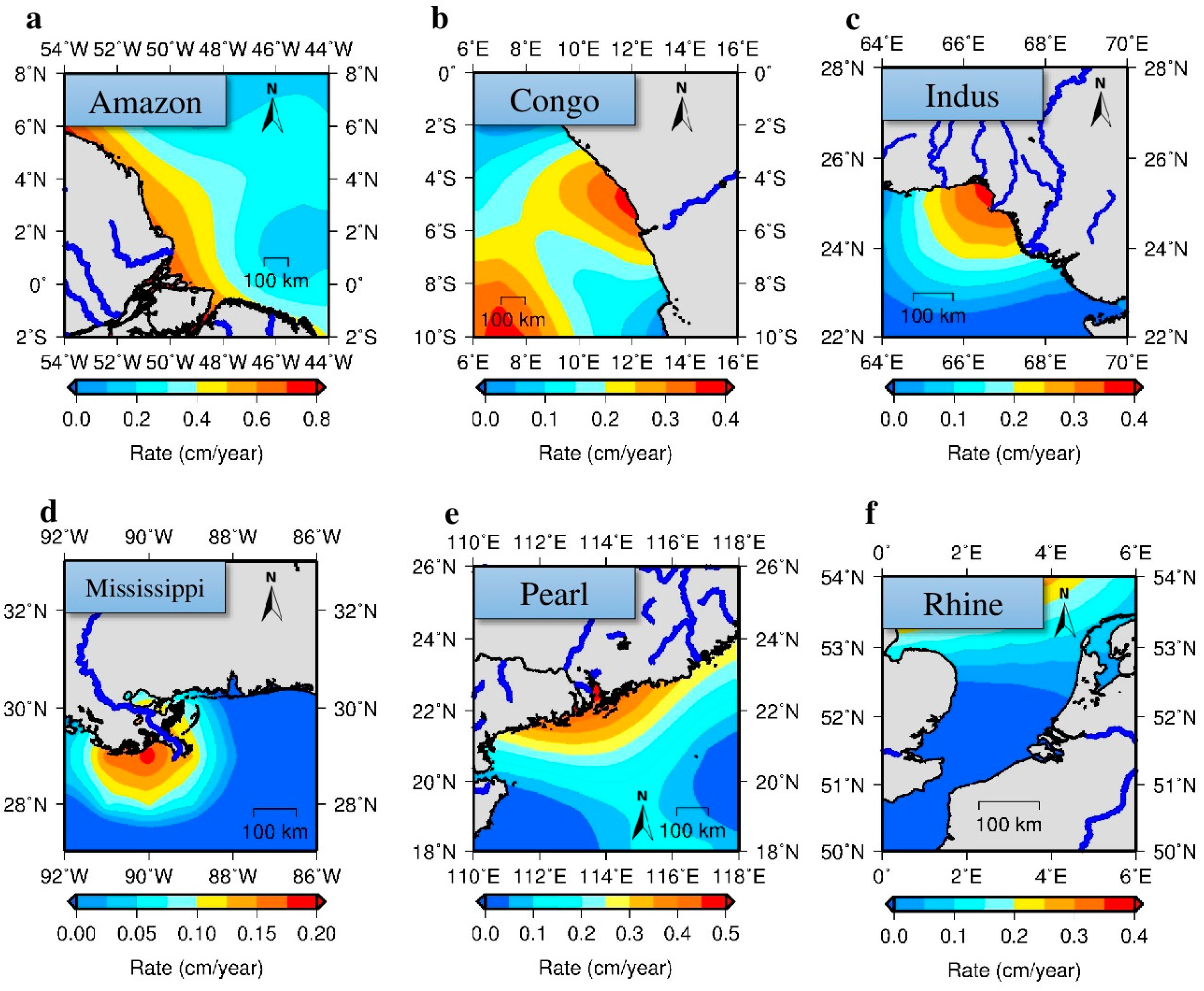
4. Discussion: Can We Detect MARS by GRACE in the World’s Major Estuaries?
5. Conclusions
Acknowledgments
Author Contributions
Conflicts of Interest
References
- Chen, X.; Zong, Y.; Zhang, E.; Xu, J.; Li, S. Human impacts on the Changjiang (Yangtze) River Basin, China, with special reference to the impacts on the dry season water discharges into the sea. Geomorphology 2001, 41, 111–123. [Google Scholar] [CrossRef]
- Holeman, J.N. The sediment yield of major rivers of the world. Water Resour. Res. 1968, 4, 737–747. [Google Scholar] [CrossRef]
- Xian, Q.; Ramu, K.; Isobe, T.; Sudaryanto, A.; Liu, X.; Gao, Z.; Takahashi, S.; Yu, H.; Tanabe, S. Levels and body distribution of polybrominated diphenyl ethers (PBDEs) and hexabromocyclododecanes (HBCDs) in freshwater fishes from the Yangtze River, China. Chemosphere 2008, 71, 268–276. [Google Scholar] [CrossRef] [PubMed]
- Milliman, J.D.; Meade, R.H. World-wide delivery of river sediment to the oceans. J. Geol. 1983, 91, 1–21. [Google Scholar] [CrossRef]
- Deng, B.; Zhang, J.; Wu, Y. Recent sediment accumulation and carbon burial in the East China Sea. Glob. Biogeochem. Cycles 2006. [Google Scholar] [CrossRef]
- Xu, K.; Milliman, J.D.; Li, A.; Paul Liu, J.; Kao, S.J.; Wan, S. Yangtze- and Taiwan-derived sediments on the inner shelf of East China Sea. Cont. Shelf Res. 2009, 29, 2240–2256. [Google Scholar] [CrossRef]
- Dai, S.B.; Lu, X.X. Sediment load change in the Yangtze River (Changjiang): A review. Geomorphology 2014, 215, 60–73. [Google Scholar] [CrossRef]
- Liu, J.P.; Li, A.C.; Xu, K.H.; Velozzi, D.M.; Yang, Z.S.; Milliman, J.D.; DeMaster, D.J. Sedimentary features of the Yangtze River-derived along-shelf clinoform deposit in the East China Sea. Cont. Shelf Res. 2006, 26, 2141–2156. [Google Scholar] [CrossRef]
- Su, C.C.; Huh, C.A. 210Pb, 137Cs and 239, 240Pu in East China Sea sediments: Sources, pathways and budgets of sediments and radionuclides. Mar. Geol. 2002, 183, 163–178. [Google Scholar] [CrossRef]
- Huh, C.A.; Su, C.C. Sedimentation dynamics in the East China Sea elucidated from 210Pb, 137Cs and 239, 240Pu. Mar. Geol. 1999, 160, 183–196. [Google Scholar] [CrossRef]
- Tapley, B.D.; Bettadpur, S.; Ries, J.C.; Thompson, P.F.; Watkins, M.M. GRACE measurements of mass variability in the Earth system. Science 2004, 305, 503–505. [Google Scholar] [CrossRef] [PubMed]
- Velicogna, I.; Wahr, J. Greenland mass balance from GRACE. Geophys. Res. Lett. 2005, 32, L18505. [Google Scholar] [CrossRef]
- Velicogna, I.; Wahr, J. Measurements of time-variable gravity show mass loss in Antarctica. Science 2006, 311, 1754–1756. [Google Scholar] [CrossRef] [PubMed]
- Rodell, M.; Velicogna, I.; Famiglietti, J.S. Satellite-based estimates of groundwater depletion in India. Nature 2009, 460, 999–1002. [Google Scholar] [CrossRef] [PubMed]
- Feng, W.; Zhong, M.; Lemoine, J.-M.; Biancale, R.; Hsu, H.T.; Xia, J. Evaluation of groundwater depletion in North China using the Gravity Recovery and Climate Experiment (GRACE) data and ground-based measurements. Water Resour. Res. 2013, 49, 2110–2118. [Google Scholar] [CrossRef]
- Chambers, D.P.; Bonin, J.A. Evaluation of Release-05 GRACE time-variable gravity coefficients over the ocean. Ocean Sci. 2012, 8, 859–868. [Google Scholar] [CrossRef]
- Tregoning, P.; Lambeck, K.; Ramillien, G. GRACE estimates of sea surface height anomalies in the Gulf of Carpentaria, Australia. Earth Planet. Sci. Lett. 2008, 271, 241–244. [Google Scholar] [CrossRef]
- Wouters, B.; Chambers, D. Analysis of seasonal ocean bottom pressure variability in the Gulf of Thailand from GRACE. Glob. Planet. Chang. 2010, 74, 76–81. [Google Scholar] [CrossRef]
- Feng, W.; Lemoine, J.M.; Zhong, M.; Hsu, H.T. Mass-induced sea level variations in the Red Sea from GRACE, steric-corrected altimetry, in situ bottom pressure records, and hydrographic observations. J. Geodyn. 2014, 78, 1–7. [Google Scholar] [CrossRef]
- Bettadpur, S. Level-2 Gravity Field Product User Handbook. Available online: ftp://podaac.jpl.nasa.gov/allData/grace/docs/L2-UserHandbook_v3.0.pdf (accessed on 26 May 2016).
- Flechtner, F.; Dobslaw, H.; Fagiolini, E. AOD1B Product Description Document for Product Release 05 (Rev. 4.4). Available online: ftp://podaac.jpl.nasa.gov/allData/grace/docs/AOD1B_PDD_v4.4.pdf (accessed on 24 March 2016).
- Chen, J.L.; Rodell, M.; Wilson, C.R.; Famiglietti, J.S. Low degree spherical harmonic influences on Gravity Recovery and Climate Experiment (GRACE) water storage estimates. Geophys. Res. Lett. 2005. [Google Scholar] [CrossRef]
- Swenson, S.; Chambers, D.; Wahr, J. Estimating geocenter variations from a combination of GRACE and ocean model output. J. Geophys. Res. 2008. [Google Scholar] [CrossRef]
- Cheng, M.; Ries, J.C.; Tapley, B.D. Variations of the Earth’s figure axis from satellite laser ranging and GRACE. J. Geophys. Res. 2011, 116, B01409. [Google Scholar] [CrossRef]
- Swenson, S.; Wahr, J. Post-processing removal of correlated errors in GRACE data. Geophys. Res. Lett. 2006. [Google Scholar] [CrossRef]
- Tangdamrongsub, N.; Hwang, C.; Shum, C.K.; Wang, L. Regional surface mass anomalies from GRACE KBR measurements: Application of L-curve regularization and a priori hydrological knowledge. J. Geophys. Res. 2012. [Google Scholar] [CrossRef]
- Wahr, J.; Molenaar, M.; Bryan, F. Time variability of the Earth’s gravity field: Hydrological and oceanic effects and their possible detection using GRACE. J. Geophys. Res. 1998, 103, 30205–30229. [Google Scholar] [CrossRef]
- Guo, J.Y.; Duan, X.J.; Shum, C.K. Non-isotropic Gaussian smoothing and leakage reduction for determining mass changes over land and ocean using GRACE data. Geophys. J. Int. 2010, 181, 290–302. [Google Scholar] [CrossRef]
- Bonin, J.; Chambers, D. Uncertainty estimates of a GRACE inversion modelling technique over Greenland using a simulation. Geophys. J. Int. 2013, 194, 212–229. [Google Scholar] [CrossRef]
- Tangdamrongsub, N.; Hwang, C.; Kao, Y.C. Water storage loss in central and South Asia from GRACE satellite gravity: correlations with climate data. Nat. Hazards 2011, 59, 749–769. [Google Scholar] [CrossRef]
- Rodell, M.; Houser, P.R.; Jambor, U.; Gottschalck, J.; Mitchell, K.; Meng, C.J.; Arsenault, K.; Cosgrove, B.; Radakovich, J.; Bosilovich, M.; et al. The global land data assimilation system. Bull. Am. Meteorol. Soc. 2004, 85, 381–394. [Google Scholar] [CrossRef]
- Hwang, C.; Kao, Y.C. Spherical harmonic analysis and synthesis using FFT: Application to temporal gravity variation. Comput. Geosci. 2006, 32, 442–451. [Google Scholar] [CrossRef]
- Yi, S.; Wang, Q.; Sun, W. Basin mass dynamic changes in China from GRACE based on a multibasin inversion method. J. Geophys. Res. Solid Earth. 2016. [Google Scholar] [CrossRef]
- Sakumura, C.; Bettadpur, S.; Bruinsma, S. Ensemble prediction and intercomparison analysis of GRACE time-variable gravity field models. Geophys. Res. Lett. 2014, 41, 1389–1397. [Google Scholar] [CrossRef]
- Trenberth, K.E.; Smith, L.; Qian, T.; Dai, A.; Fasullo, J. Estimates of the global water budget and its annual cycle using observational and model data. J. Hydrometeorol. 2007, 8, 758–769. [Google Scholar] [CrossRef]
- NOAA Earth System Research Laboratory. Available online: http://www.esrl.noaa.gov/psd/enso/mei/table.html (accessed on 29 May 2016).
- Torrence, C.; Compo, G.P. A Practical Guide to Wavelet Analysis. Bull. Am. Meteorol. Soc. 1998, 79, 61–78. [Google Scholar] [CrossRef]
- Ding, Y.; Chan, J.C.L. The East Asian summer monsoon: An overview. Meteorol. Atmos. Phys. 2005, 89, 117–142. [Google Scholar]
- Chang, C.P.; Wang, Z.; Hendon, H. The Asian winter monsoon. In The Asian Monsoon; Wang, B., Ed.; Praxis Publishing Ltd.: Chichester, UK, 2006; pp. 89–127. [Google Scholar]
- Liu, J.P.; Xu, K.H.; Li, A.C.; Milliman, J.D.; Velozzi, D.M.; Xiao, S.B.; Yang, Z.S. Flux and fate of Yangtze River sediment delivered to the East China Sea. Geomorphology 2007, 85, 208–224. [Google Scholar] [CrossRef]
- Zeng, X.; He, R.; Xue, Z.; Wang, H.; Wang, Y.; Yao, Z.; Guan, W.; Warrillow, J. River-derived sediment suspension and transport in the Bohai, Yellow, and East China Seas: A preliminary modeling study. Cont. Shelf Res. 2015, 111, 112–125. [Google Scholar] [CrossRef]
- Xiao, S.; Li, A.; Liu, J.P.; Chen, M.; Xie, Q.; Jiang, F.; Li, T.; Xiang, R.; Chen, Z. Coherence between solar activity and the East Asian winter monsoon variability in the past 8000 years from Yangtze River-derived mud in the East China Sea. Palaeogeogr. Palaeoclimatol. Palaeoecol. 2006, 237, 293–304. [Google Scholar] [CrossRef]
- Su, J.L. A review of circulation dynamics of the coastal oceans near China. Acta Oceanol. Sin. 2001, 23, 1–16. (In Chinese) [Google Scholar]
- Fan, D.; Qi, H.; Sun, X.; Liu, Y.; Yang, Z. Annual lamination and its sedimentary implications in the Yangtze River delta inferred from High-resolution biogenic silica and sensitive grain-size records. Cont. Shelf Res. 2011, 31, 129–137. [Google Scholar] [CrossRef]
- Liu, K.K.; Peng, T.-H.; Shaw, P.-T.; Shiah, F.K. Circulation and biogeochemical processes in the East China Sea and the vicinity of Taiwan: An overview and a brief synthesis. Deep Sea Res. II 2003, 50, 1055–1064. [Google Scholar] [CrossRef]
- Lindzen, R.S.; Holton, J.R. A theory of the quasi-biennial oscillation. J. Atmos. Sci. 1968, 25, 1095–1107. [Google Scholar] [CrossRef]
- Pan, Y.; Shen, W.B.; Ding, H.; Hwang, C.; Li, J.; Zhang, T. The quasi-biennial vertical oscillations at global GPS stations: Identification by ensemble empirical mode decomposition. Sensors 2015, 15, 26096–26114. [Google Scholar] [CrossRef] [PubMed]
- Kim, W.; Yeh, S.-W.; Kim, J.H.; Kug, J.S.; Kwon, M. The unique 2009–2010 El Niño event: A fast phase transition of warm pool El Niño to La Niña. Geophys. Res. Lett. 2011. [Google Scholar] [CrossRef]
- Boening, C.; Willis, J.K.; Landerer, F.W.; Nerem, R.S.; Fasullo, J. The 2011 La Niña: So strong, the oceans fell. Geophys. Res. Lett. 2012, 39, L19602. [Google Scholar] [CrossRef]
- Gao, H.; Yang, S. A severe drought event in northern China in winter 2008–2009 and the possible influences of La Niña and Tibetan Plateau. J. Geophys. Res. 2009. [Google Scholar] [CrossRef]
- Mantua, N.J.; Hare, S.R.; Zhang, Y.; Wallace, J.M.; Francis, R.C. A pacific interdecadal climate oscillation with impacts on salmon production. Bull. Am. Meteorol. Soc. 1997, 78, 1069–1079. [Google Scholar] [CrossRef]
- Wong, L.A.; Chen, J.C.; Xue, H.; Dong, L.X.; Su, J.L.; Heinke, G. A model study of the circulation in the Pearl River Estuary (PRE) and its adjacent coastal waters: 1. Simulations and comparison with observations. J. Geophys. Res. 2003. [Google Scholar] [CrossRef]
- Vangriesheim, A.; Khripounoff, A.; Crassous, P. Turbidity events observed in situ along the Congo submarine channel. Deep Sea Res. 2009, 56, 2208–2222. [Google Scholar] [CrossRef]
- Hsu, K.J.; Weissert, H.J. South Atlantic Paleoceanography; Cambridge University Press: Cambridge, UK, 1985. [Google Scholar]
- Millian, J.D.; Farnsworth, K.L. River Discharge to the Coastal Ocean, A Global Synthesis; Cambridge University Press: Cambridge, UK, 2013. [Google Scholar]


| Effect | CSR | JPL | GFZ |
|---|---|---|---|
| Solid Earth tide | IERS-2010 | IERS-2003 | IERS-2010 |
| Ocean tide | GOT4.8, FES2004 | GOT4.7, SCEQ | EOT11a |
| Pole tide | IERS-2010 (cubic) | IERS-2003 (linear) | IERS-2010 (cubic) |
| Ocean pole tide | Self-consistent equilibrium model | No | No |
| Indirect J2 effect | Sun, Moon | Moon | Moon |
| Non-tidal oceanic loading | OMCT (for all centres) | ||
| Non-tidal atmospheric loading | ECMWF (for all centres) | ||
| CSR | JPL | GFZ | Mean | |
|---|---|---|---|---|
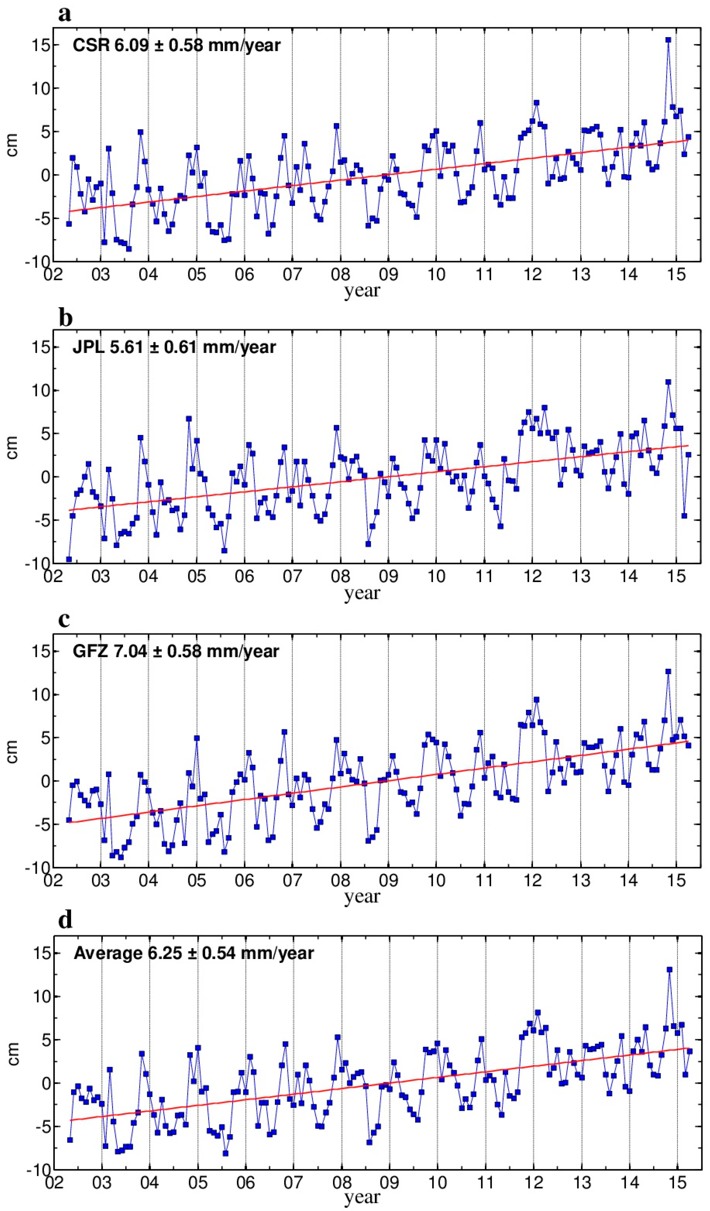
| Rate of EWH (mm/year) | 6.09 | 7.04 | 5.61 | 6.25 |
| Rate of mass change (×109 ton/year) | 1.31 | 1.51 | 1.21 | 1.34 |
© 2016 by the authors; licensee MDPI, Basel, Switzerland. This article is an open access article distributed under the terms and conditions of the Creative Commons Attribution (CC-BY) license (http://creativecommons.org/licenses/by/4.0/).
Share and Cite
Liu, Y.-C.; Hwang, C.; Han, J.; Kao, R.; Wu, C.-R.; Shih, H.-C.; Tangdamrongsub, N. Sediment-Mass Accumulation Rate and Variability in the East China Sea Detected by GRACE. Remote Sens. 2016, 8, 777. https://0-doi-org.brum.beds.ac.uk/10.3390/rs8090777
Liu Y-C, Hwang C, Han J, Kao R, Wu C-R, Shih H-C, Tangdamrongsub N. Sediment-Mass Accumulation Rate and Variability in the East China Sea Detected by GRACE. Remote Sensing. 2016; 8(9):777. https://0-doi-org.brum.beds.ac.uk/10.3390/rs8090777
Chicago/Turabian StyleLiu, Ya-Chi, Cheinway Hwang, Jiancheng Han, Ricky Kao, Chau-Ron Wu, Hsuan-Chang Shih, and Natthachet Tangdamrongsub. 2016. "Sediment-Mass Accumulation Rate and Variability in the East China Sea Detected by GRACE" Remote Sensing 8, no. 9: 777. https://0-doi-org.brum.beds.ac.uk/10.3390/rs8090777