Next Article in Journal
Intercomparison of XH2O Data from the GOSAT TANSO-FTS (TIR and SWIR) and Ground-Based FTS Measurements: Impact of the Spatial Variability of XH2O on the Intercomparison
Next Article in Special Issue
Assessing Orographic Variability in Glacial Thickness Changes at the Tibetan Plateau Using ICESat Laser Altimetry
Previous Article in Journal
Investigation of Urbanization Effects on Land Surface Phenology in Northeast China during 2001–2015
Previous Article in Special Issue
Modeling and Reconstruction of Time Series of Passive Microwave Data by Discrete Fourier Transform Guided Filtering and Harmonic Analysis
 
 
Addendum published on 16 February 2017, see Remote Sens. 2017, 9(2), 157.
Article

Evaluation of Methods for Aerodynamic Roughness Length Retrieval from Very High-Resolution Imaging LIDAR Observations over the Heihe Basin in China

1
ICube Laboratory, UMR 7357 CNRS-University of Strasbourg, F-67412 Illkirch Cedex, France
2
Department of Geoscience and Remote Sensing (GRS), Delft University of Technology, 2628 CN Delft, The Netherlands
3
State Key Laboratory of Remote Sensing Science, Institute of Remote Sensing and Digital Earth, Chinese Academy of Sciences, Beijing 100101, China
*
Author to whom correspondence should be addressed.
Submission received: 30 June 2016 / Revised: 21 December 2016 / Accepted: 31 December 2016 / Published: 12 January 2017

Abstract

:
The parameterization of heat transfer based on remote sensing data, and the Surface Energy Balance System (SEBS) scheme to retrieve turbulent heat fluxes, already proved to be very appropriate for estimating evapotranspiration (ET) over homogeneous land surfaces. However, the use of such a method over heterogeneous landscapes (e.g., semi-arid regions or agricultural land) becomes more difficult, since the principle of similarity theory is compromised by the presence of different heat sources at various heights. This study aims to propose and evaluate some models based on vegetation geometry partly developed by Colin and Faivre, to retrieve the surface aerodynamic roughness length for momentum transfer ( z 0 m ), which is a key parameter in the characterization of heat transfer. A new approach proposed by the authors consisted in the use of a Digital Surface Model (DSM) as boundary condition for experiments with a Computational Fluid Dynamics (CFD) model to reproduce 3D wind fields, and to invert them to retrieve a spatialized roughness parameter. Colin and Faivre also applied the geometrical Raupach’s approach for the same purpose. These two methods were evaluated against two empirical ones, widely used in Surface Energy Balance Index (SEBI) based algorithms (Moran; Brutsaert), and also against an alternate geometrical model proposed by Menenti and Ritchie. The investigation was carried out in the Yingke oasis (China) using very-high resolution remote sensing data (VNIR, TIR & LIDAR), for a precise description of the land surface, and a fine evaluation of estimated heat fluxes based on in-situ measurements. A set of five numerical experiments was carried out to evaluate each roughness model. It appears that methods used in experiments 2 (based on Brutsaert) and 4 (based on Colin and Faivre) are the most accurate to estimate the aerodynamic roughness length, according to the estimated heat fluxes. However, the formulation used in experiment 2 allows to minimize errors in both latent and sensible heat flux, and to preserve a good partitioning. An additional evaluation of these two methods based on another k B 1 parameterization could be necessary, given that the latter is not always compatible with the CFD-based retrieval method.

Graphical Abstract

1. Introduction

Remote sensing, with its capability of large spatial and frequent temporal coverage, has become a widely used and powerful tool to monitor land and environmental changes. Land surface properties retrieved from Earth Observation (EO) in the optical spectral domain from visible, near-infrared to thermal infrared) are used in many models dealing with hydrological, meteorological and ecological processes. The estimation and monitoring of evapotranspiration (ET) by remote sensing has also become a common application.
Some of the proposed energy balance algorithms allow partitioning of turbulent flow between a wet and dry limit expressed by the normalized temperature gradient between the surface and the atmosphere at a reference level [1]. This concept proposed by Menenti and Choudhury [2] is called Surface Energy Balance Index (SEBI), and the boundary conditions are either observed [3,4] or calculated [5,6,7]. This type of approach already proved to be efficient for estimating the surface energy balance and relatively easy to implement.
The algorithm called Surface Energy Balance System (SEBS) formulated by Su [5] is a parameterization scheme based on the concept of SEBI, which is known for its use both locally and regionally, and for any condition of atmospheric stability. The combination of remote sensing data acquired in the visible, near infrared (albedo, leaf area index, fractional vegetation cover) and thermal infrared (land surface temperature) with the measurement of radiation at the surface and atmospheric variables at reference level (temperature, wind speed, specific humidity) allows to calculate the actual temperature gradients as well as the wet and dry limits, between the surface and the atmosphere for each pixel. Su [5] adapts the choice of stability functions depending on whether the reference level considered is located in the surface layer or in the mixing layer [8].
Independently of the measurement errors related to the different atmospheric variables or models to retrieve surface parameters (temperature, albedo, leaf area index, among others), SEBS is sensitive to the parameterization of the aerodynamic resistance ( r a h ), i.e., resistance to the heat transfer in a layer of atmosphere. The expression of resistance requires the calculation of aerodynamic roughness length for heat transfer ( z 0 h ), estimated from the aerodynamic roughness length for momentum transfer ( z 0 m ) through the k B 1 model [9]. z 0 m is used to scale the logarithmic increase of wind speed with height in a neutrally stratified layer from a level of no motion near the surface. Furthermore, z 0 m should be experimentally determined from wind velocity and air temperature profiles. Such resulting roughness estimates are found to be in good agreement with the relationships linking the geometric and the aerodynamic roughness. This suggests that for natural surfaces z 0 m can be estimated on the basis of the geometric characteristics of the roughness elements.
According to the studies by Arya [10], Andreas [11], Oke [12] and Stull [13], the dimensions, and density distribution of surface roughness elements are influential on z 0 m . Due to increasing height, surface area and density of roughness elements, the value of z 0 m increases, until the ratio between the silhouette area (upwind face of elements) and unit ground area reaches 0.4. After this value, a transition to “skimming” flow occurs and z 0 m starts to decrease again [14,15]. The standard method to derive z 0 m is from the vertical profile of horizontal wind speed, using measurements at two or more heights in the atmospheric boundary layer (ABL).
In the past decades, there have been two main acceptable strategies to estimate the aerodynamic roughness. On one hand, in situ measurements dependent on the bulk transfer equations [16]. On the other hand, the studies done by Menentie and Ritchie [17], Su et al. [18] and De Vries et al. [19] documented that z 0 m can be estimated with measurements by laser scanning and optical remote sensing. However, the roughness models for z 0 m retrieval used in SEBS are defined from empirical relationships generally based on the Normalized Difference Vegetation Index (NDVI) and for specific and uniform vegetation [20,21]. Their use for the characterization of heterogeneous surfaces is outside from their domain of validity, sometimes leading to a significant degradation of turbulent flux estimates [22]. Moreover, these models do not take into account the dynamic aspect of the roughness length: the rapid change of wind speed and direction in a local context with the presence of obstacles may result in a significant temporal variability. Su et al. [18] then recognize that the use of models to estimate roughness length is not always appropriate in the sense that they ignore the flow history of an air mass over heterogeneous areas.
These approaches would benefit from the combined use of passive remote sensing and land surface structure measurements from Light Detection And Ranging (LIDAR) techniques. Since the very early use of laser altimetry [23], sensor performances have significantly improved, allowing airborne profiler to be used to derive the roughness of the surface [17]. More recently, satellite and airborne imaging LIDAR systems have paved the way to the mapping of vegetation properties over forest areas [24], sometimes associated with complex topography [25], but also on low vegetation like salt-marshes [26] or semi-arid steppes [27].
Colin and Faivre [28] locally characterized the surface geometry using a Digital Surface Model (DSM) obtained by the acquisition from an airborne imaging LIDAR system. The introduction of the surface model in a Computational Fluid Dynamics (CFD) model allowed to generate a 3D wind field. The inversion of wind vertical profiles enable to produce a 2D mapping of aerodynamic roughness length for momentum transfer. Two geometrical approaches which account for wind direction were also applied to the digital surface model [29,30]. This study aims to evaluate the reliability and accuracy of geometrical models and the CFD-based method for roughness length retrieval proposed by Colin and Faivre [28]. Hence, these methods will be compared to three other simpler formulations which correspond to a static definition of z 0 m . The assessment will be performed through various SEBS calculations of turbulent heat fluxes integrating the respective spatialized roughness values. The performance of each method will be determined by comparing results with ground measurements of heat fluxes. Moreover, SEBS calculations require the combination of land surface properties, such as albedo, radiative temperature, emissivity, Leaf Area Index (LAI) and fractional vegetation cover ( f c ); and atmospheric measurements (air temperature, wind speed and specific humidity). Land surface variables have to be retrieved from very high-resolution visible and near-infrared (VNIR) to thermal infrared (TIR) remotely sensed observations.
This document first presents the theoretical background that underlies both SEBS algorithm [5] and roughness retrieval methods proposed by Colin and Faivre [28] (Section 2). Then, the addressed study area and materials are detailed (Section 3), land surface parameters and the additional roughness length retrieval methods are also described (Section 4). Two evaluations of all the z 0 m retrieval methods are then performed (Section 5 and Section 6) and results are discussed in Section 7.

2. Theoretical Background

2.1. Energy Balance at the Land Surface

Taking the land surface as a flat and thin layer such that no heat storage exists, the surface energy balance equation at the interface between the land surface and the overlying atmosphere is written as:
R n = H + λ E + G 0
where R n is the net radiation flux, H is the sensible heat flux, λ E is the latent heat flux and G 0 is the soil heat flux. The sign convention in Equation (1) is that R n is considered positive when directed towards the land surface, while H, λ E and G 0 are considered positive when directed away from the land surface. For the sake of simplicity, all flux densities will be called fluxes, and the unit is W/m 2 .
The soil heat flux is often parameterized proportionally to the net radiation arriving at the soil surface, therefore is function of the fractional vegetation cover [31,32,33]. It can be expressed as:
G 0 = R n × ( Γ c + ( 1 f c ) × ( Γ s Γ c ) )
in which it is assumed that the ratio of soil heat flux to net radiation Γ c = 0.05 for full vegetation canopy [34] and Γ s = 0.315 for bare soil [35]. An interpolation is then performed between these limiting cases using the fractional vegetation cover ( f c ).

2.2. Parameterization of Turbulent Heat Fluxes

In the context of applying remote sensing measurements to estimate heat fluxes, the latent heat flux (or evaporation when expressed in term of water depth) is calculated as the residual of energy balance (Equation (1)) and the major concern is to calculate sensible heat flux by a proper parameterization of resistance for heat transfer r a h . The sensible heat flux is related to the difference between the surface radiative temperature T 0 and air temperature T a at a reference height z within surface layer by a bulk transfer equation [34]:
H = ρ a c p T 0 T a r a h
where ρ a is the air density (kg/m 3 ), c p is the heat capacity of the air (J/kg/K), r a h is the aerodynamic resistance for heat transfer (s/m) between the surface and the reference height (z) in the Atmospheric Surface Layer (ASL), usually estimated on the basis of similarity theory. The aerodynamic resistance for heat transfer r a h is given by [8,34]:
r a h = 1 k u * l n z d 0 z 0 h ψ h z d 0 L + ψ h z 0 h L
where k is the Von Karman constant (k = 0.4), d 0 is the displacement height (m), z 0 h the roughness length for heat transfer (m), ψ h is the Monin-Obukhov stability correction function for heat transfer, and u * is the friction velocity (m/s) in the ASL (defined as ( τ 0 / ρ a ) 1 / 2 with τ 0 the surface shear stress) and is expressed as:
u * = k u z l n z d 0 z 0 m ψ m z d 0 L + ψ m z 0 m L
with z 0 m the roughness length for momentum transfer (m), ψ m is the Monin-Obukhov stability correction function for momentum transfer, and L in Equations (4) and (5) is the Monin-Obukhov length given as:
L = ρ a c p u * 3 θ a v k g H
where θ a v is the potential virtual air temperature near the surface (K). The roughness length for heat transfer z 0 h can be derived from the k B 1 , which is defined by the ratio z 0 m over z 0 h as [36,37]:
k B 1 = l n z 0 m z 0 h
where B is the dimensionless parameter introduced by Chamberlain [36] and used by Owen and Thomson [37]. To estimate the k B 1 , SEBS relies on a dynamic model for thermal roughness length calculation adapted from Massman [9], Su et al. [18] and Su [5]. In this model, the k B 1 parameter is expressed as a function of surface conditions and of aerodynamic parameters:
k B 1 = k C d 4 C t u * u ( h v ) ( 1 e n / 2 ) f c 2 + k u * u ( h v ) z 0 m h v C t * 2 f c f s + k B s 1 f s 2
where C d is the drag coefficient of the foliage elements and is set to 0.2 [5], f c is the fractional vegetation coverage and f s is its complement, C t is the heat transfer coefficient of the leaf ranging in 0.005 N C t 0.0074 N (N is number of sides of a leaf to participate in heat exchange), n is the windspeed extinction coefficient within the canopy, h v the vegetation height, C t * the heat transfer coefficient of the soil and is given by C t * = P r 2 / 3 R e * 1 / 2 , where P r is the Prandtl number: 0.71 [9] and the roughness Reynolds number R e 1 / 2 = h s u * / ν , with h s the roughness height of the soil, k B s 1 is the value of k B 1 for bare soil surface [38].
Su [5] has proposed the Surface Energy Balance System (SEBS) by extending the SEBI concept [2] with a dynamic model for thermal roughness [18], the Bulk Atmospheric Similarity (BAS) theory of Brutsaert [8] for PBL scaling and the Monin-Obukhov Atmospheric Surface Layer (ASL) similarity for surface layer scaling. This allows SEBS to be used for both local scaling and regional scaling under all atmospheric stability regimes, providing a link for radiometric measurements and atmospheric models at various scales.
In SEBS, the concept that actual evapotranspiration is regulated by its two extreme limits as used in SEBI is extended to the sensible flux. So, actual sensible heat flux H is constrained in the range set by the sensible heat flux at the wet limit H w (the low limit in SEBI) and the sensible heat flux at the dry limit H d (the upper limit in SEBI). The partitioning of turbulent heat fluxes on the basis of energy balance at limiting cases is detailed by Su [5].

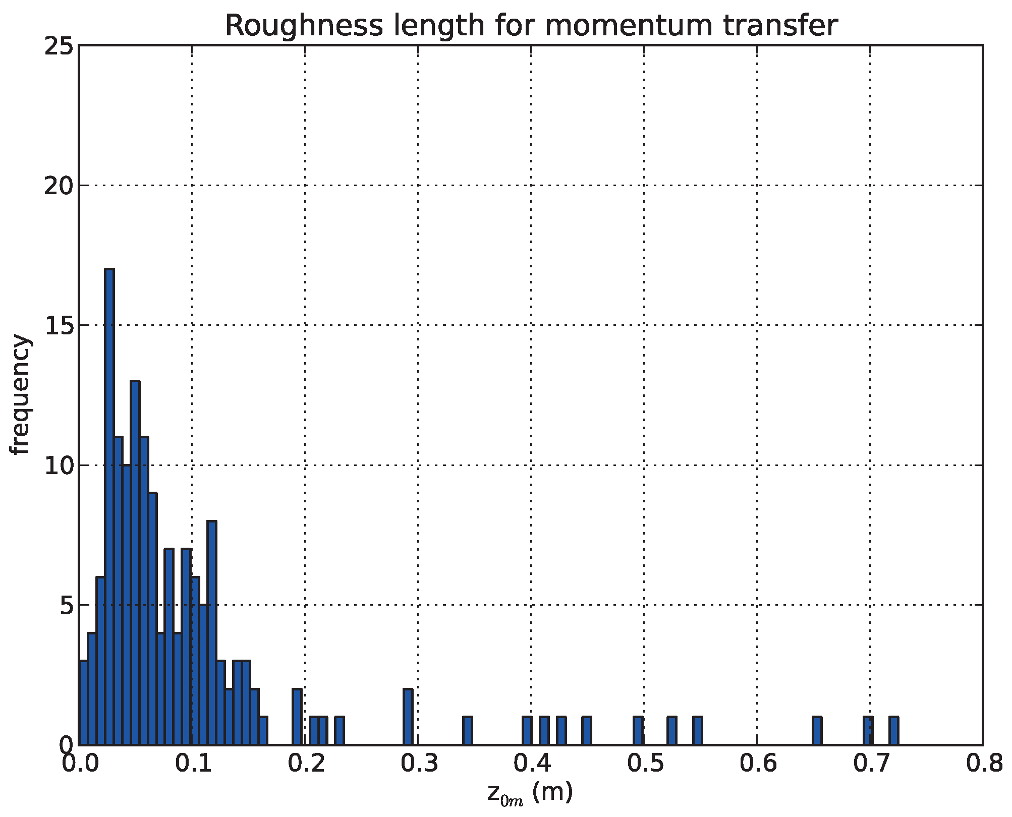
2.3. Characterization of the Surface Roughness

The wind velocity profile over the land surface with a neutral atmospheric stratification is a simple logarithmic expression of the form:
u ( z ) = u * k × ln z d 0 z 0 m
Roughness length is usually expressed as a constant ratio of the canopy height for homogeneous surfaces like continuous low vegetation canopies, with a consensus for values of around z 0 m / h v 0.1 [38]. However, the homogeneity assumption is generally never met. Therefore, such kind of approximation is of limited interest for most environmental studies.

2.3.1. Geometry of Canopy to Parameterize Aerodynamic Roughness

It has long been demonstrated from field work and wind tunnel experiments that the drag affecting the airflow over a heterogeneous land surface is related to roughness elements density and size [39,40]. This was expressed in the formulation proposed by Lettau [41]:
z 0 m = 0.5 × h × λ f
where h is an effective averaged obstacle height, and λ f is the frontal area index defined as:
λ f = A f A T
The frontal area index expresses the ratio of the frontal area A f (perpendicular to the flow) over the total area covered by roughness elements A T . A well-known formulation based on the combined use of h and λ f was proposed by Raupach [29] to calculate the displacement height d 0 and the roughness length z 0 m . Raupach’s formulation of the displacement height is:
d 0 h v = 1 1 exp C dl 2 λ f 0.5 C dl 2 λ f 0.5
and the formulation of the roughness length is:
z 0 m h v = 1 d 0 h v × exp k U u * + ψ h
with
u * U = min C s + C R λ f 0.5 ; u * U max
where ϋ h expresses the influence of the roughness sublayer, C s is the drag coefficient for an obstacle free surface, C R the drag coefficient for an isolated obstacle, and C dl a free parameter [29]. In this study, we used values recommended by Raupach [29], i.e., the values of ψ h = 0.193, C s = 0.003, C R = 0.3, C dl = 7.5 and u * / U max = 0.3.
Colin and Faivre [28] implemented a second geometrical approach based on the work of Theurer [42], quoted by MacDonald et al. [30], where z 0 m and d 0 could be also estimated by combining the frontal area index with the plan area index. Since these two approaches provide very similar z 0 m values [28], only the Raupach’s formulation is retained in this study.

2.3.2. Modeling Air Flow

The direct use of both Digital Elevation and Surface Models (DEM & DSM) in a Computational Fluid Dynamics (CFD) solver was explored by Colin and Faivre [28]. The CFD solver called Canyon, embedded in the WindStation software [43], allows for numerical simulations of turbulent flows over complex topography, and can account for the geometry of surface roughness elements through the Digital Surface Model, as obtained from LIDAR data. The solver follows a control-volume approach, and solves for mass conservation, momentum conservation following Navier-Stokes equations, and also energy conservation for non-neutral situations. 3D wind fields obtained by CFD modeling express the combined effect of topography and roughness elements on the airflow, and result from the solution of the transport equation. Therefore an aerodynamic roughness length is obtained from the wind profile of each computation grid by inverting Equation (9) with values within the ground and a given elevation [28].

3. Study Area and Materials

3.1. Heihe River Basin and the Yingke Oasis

The study area is located in the Heihe river basin, this area is a typical inland river basin in the northwest of China (Figure 1a,b). The second largest inland river basin of the country, it is located between 97 24 –102 10 E and 37 41 –42 42 N, and covers an area of approximately 130,000 km 2 . Experiments conducted in the scope of the Watershed Allied Telemetry Experimental Research (WATER) project consisted in simultaneous airborne, satellite-borne and ground-based remote sensing measurements aiming at improving the observability, understanding and predictability of hydrological and ecological processes at catchment scale [44]. Airborne data used in this study were acquired over the Yingke oasis, located to the south of the Zhangye city (100 25 E, 38 51 N, 1519 m a.s.l.), which is a typical irrigated farmland (Figure 1c) where the primary crops are maize and wheat, with fields often separated by tree rows.

3.2. Airborne VNIR & TIR Radiometric Data

The Wide-Angle Dual-mode Line/Area Array Scanner (WiDAS) is composed of two thermal imagers and four CCD cameras [44]. The thermal imager has two bands (3.5–5 and 8–12 μ m) with an array of 320 per 240 pixels, an 80 total field of view (FOV) divided into seven observation angles: +40 , +30 , +20 , 0 , −20 , −30 , −40 (+ as forward, − as backward). The CCD camera has four bands (centered at 550, 650, 700 and 750 nm), a detector array of 1392 per 1040 pixels, a 60 total field of view and five observation angles: +30 , +20 , 0 , −20 , −30 .
Brightness temperature of land surface is provided by the radiance measured in the 8–12 μ m band after atmospheric correction. Radiances for visible and thermal infrared domains were both corrected using MODTRAN4 [45] on the basis of ABL soundings acquired at the time of the airborne survey. Spectral reflectances are used to derive land surface properties.

3.3. Airborne LIDAR

The WATER field campaign included an intensive observation period. Twenty-five missions were flown in 2008 with different sensors. We used the data collected by a LiteMapper 5600 imaging LIDAR, whose major characteristics are a wavelength of 1550 nm, a pulse of 3.5 ns at 100 kHz and a scan angle range of ±22.5 [44]. The spatial density for a flight height of 800 m above the ground is 4 impacts per square meter. After correction of the raw data to account for the attitude of the plane and for the precise location of the sensor, each return signal can be translated into an accurate 3D georeferenced point. The resulting point cloud is then processed to extract the minimum and maximum elevation from the points in each square meter grid. The lowest elevation point is used to derive the elevation of the ground. After removing local aberrations, the resulting map is a Digital Elevation Model (DEM), expressed in terms of altitude above mean sea level (a.m.s.l), in meters. If the surface is a solid block, or a bare soil, the minimum and maximum elevation values are equivalent. However, for sparse vegetation structures, the difference between the lowest and highest elevations reflects the height of the vegetation canopy. Therefore, it is possible to separate the land surface topography, represented by the DEM, from the elevation of the top of the vegetation canopy. The latter is called the Digital Surface Model (DSM), and is also expressed in terms of altitude a.m.s.l. Both digital models have a spatial resolution of 1 m. The LIDAR flight was operated the 20 June 2008, and the scene covers an area of 7.2 km 2 (Figure 2).

3.4. Meteorological Data

The Yingke oasis experimental site is permanently instrumented with an Automatic Meteorological Station (AMS). The AMS records every ten minutes the air temperature, wind speed and direction at 2 and 10 m, air pressure, relative humidity, precipitation, net radiation, soil heat flux, soil temperature and water content. Moreover, latent heat flux, sensible heat flux and water vapor concentration are obtained from Eddy Covariance (EC) system with an integration step of 30 min. Surface observation of heat fluxes by EC systems captures fluxes originating from a limited source area, which depends on the observation height, atmospheric and surface conditions. The source area has to be properly located and delineated when comparing pixel-based remote sensing estimates of heat fluxes with ground measurements. The concept of footprint or source weight function is used as the contribution, per unit surface flux, of each unit element of the upwind surface area to a measured vertical flux [46]. The EC footprints applying to actual conditions can be employed in validating the surface heat fluxes estimated with multispectral satellite data over a range of spatial resolutions. Details about the footprint model applied to the EC measurements performed at the Yingke station are given by Colin et al. [47]. The EC systems used during the WATER experiment were initially installed at the same location to evaluate their relative accuracy [44,47].

4. Characterization of the Land Surface

The parameterization of turbulent heat fluxes at the local scale involves the preparation of the radiometric data acquired by the WiDAS sensor, following the SEBS algorithm requirements. A single input dataset of land surface variables is produced, and only the surface geometrical characterization will vary in the different calculations, in order to evaluate the various roughness length parameterization methods, including some empirical relationships.

4.1. Land Surface Parameters Retrieval

Land surface properties such as albedo, Normalized Difference Vegetation Index (NDVI), Leaf Area Index (LAI), fractional vegetation cover ( f c ), and Land Surface Temperature & Emissivity (LST, LSE) were retrieved from the WiDAS sensor following the methods and formulations detailed below. These land surface variables will remain constant in each experiment.

4.1.1. Albedo

Albedo corresponds to the spectral and hemispheric integral of spectral and directional reflectances over the useful solar spectrum (from 0.3 to 3 μ m). As spectral bands of the WiDAS camera do not completely cover this spectrum, a weighting coefficient for incoming solar radiation has to be calculated for each spectral band of the sensor. The portion of albedo recorded by the camera (weighted sum of the spectral reflectances) has to be fitted with an integral albedo in order to determine a linear relationship. Using spectral signatures of several surfaces from ASTER (Advanced Spaceborne Thermal Emission and Reflection Radiometer) libraries, and corresponding to the land cover of the study area, a total albedo is computed for each of them (integrated on the entire useful solar spectrum) and normalized by the incoming solar radiation. Then for each surface, spectral reflectances are computed using the filter functions of the camera, and weighted by the corresponding solar spectrum interval. A linear regression provides the fitting function for total albedo retrieval ( y = 1.11 x 0.02 , r 2 = 0.96 ).

4.1.2. Normalized Difference Vegetation Index

The Normalized Difference Vegetation Index (NDVI) is given by:
N D V I = ρ n i r ρ r e d ρ n i r + ρ r e d
where ρ n i r and ρ r e d are the at-surface reflectances obtained from sensor bands located respectively in the near infrared (NIR) and red spectral regions. WiDAS bands 4 (0.75 μ m, NIR) and 2 (0.65 μ m, red) can be then used to obtain the NDVI. From NDVI, other surface parameters such as Leaf Area Index and fractional vegetation cover are derived.

4.1.3. Leaf Area Index

The Leaf Area Index (LAI) is the leaf area per unit ground area (m 2 /m 2 ). This variable is required for k B 1 computation with the Massman’s model (Equation (8)), and can be estimated as [48]:
L A I = N D V I × 1 + N D V I 1 N D V I 0.5
The estimation of LAI based on passive optical remote sensing would be more accurate by extending to the shortwave infrared (SWIR) domain, and by using hyperspectral data [49]. Hence, the method proposed in Equation (16) is less rigorous than ground optical passive measurements, performed with a ceptometer for instance. However, LAI is difficult to directly acquire for large spatial extents due to its time consuming and work intensive nature. Terrestrial observations are also highly sensitive to the effect of branches and stems blocking the light.

4.1.4. Fractional Vegetation Cover

The fractional vegetation cover ( f c ) is defined as the part of ground surface covered by vegetation. It is also required for the computation of k B 1 (Equation (8)), and for ground heat flux estimation (Equation (2)). f c has been traditionally estimated from remote sensing data using empirical relations with vegetation indices, as for example the NDVI. It has been demonstrated that f c depends linearly on NDVI [50], e.g., as:
f c = N D V I N D V I s N D V I v N D V I s
where N D V I s and N D V I v correspond to representative values of NDVI for bare soil ( f c → 0) and vegetation ( f c → 1), respectively. Other relationships, such as quadratic expressions have also been proposed [50,51], but they do not improve the results as discussed by Wittich and Hansing [52]. The main problem when applying Equation (17) is the correct estimation of N D V I s and N D V I v values. This is a critical task, since these values are region- and season-specific. Here we use the local minimum and maximum values of NDVI (i.e., within the 7.2 km 2 area), as the landscape ensure the presence of roads, buildings and dense green vegetation.

4.1.5. Land Surface Temperature and Emissivity

Land surface brightness temperature is provided by the radiance measured in the 8–12 μ m channel after atmospheric correction using MODTRAN4 [45] and Land Surface Temperature (LST) is retrieved from brightness temperature by the separation of emissivity. The latter is estimated from NDVI using the formulation of De Griend [53]:
ϵ = 1.009 + 0.047 × l n ( N D V I )

4.2. Models for Roughness Length Retrieval

The surface geometry will be characterized following five methods, and results of each are presented below. Besides the geometrical [29] and the CFD-based methods for roughness length retrieval [28], two commonly used empirical relationships are proposed. An alternate method based on Menenti and Ritchie [17] to exploit the DSM is also developed.

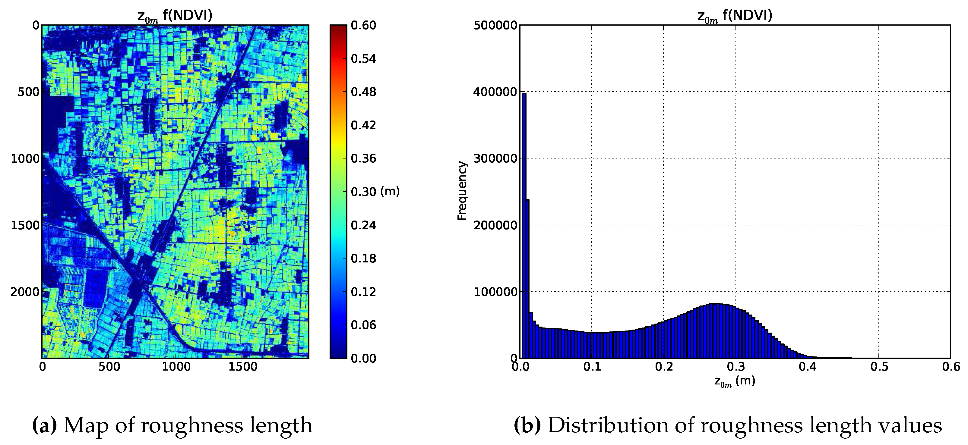
4.2.1. Roughness Length from NDVI

Some empirical formulations have been proposed to estimate roughness length for momentum transfer ( z 0 m ) from vegetation indices such as NDVI. They are generally established for a specific cover and under specific conditions, e.g., a given growing stage. Moran [20] proposed this relationship:
z 0 m = e 5.2 + 5.3 × N D V I
with the displacement height d 0 :
d 0 = z 0 m × 4.9
and the vegetation height h v :
h v = z 0 m / 0.136
Figure 3 reveals that when the surface presents high NDVI values, roughness length is larger. Using this formulation, where crops are green and dense but low, roughness values are large and on contrary where vegetation is more sparse but high, values are low. Buildings, which present negative NDVI values, are not considered as obstacles for momentum transfer. It clearly appears that this kind of formulation is not reliable in this context.

4.2.2. Roughness Length as a Fraction of Vegetation Height

Roughness length for momentum transfer can also be estimated as a simple fraction of vegetation height. In this study, taking benefits from the LIDAR digital surface model, we know the height of each obstacle around the Yingke oasis station with an horizontal resolution of 1 m. Following Brutsaert [38], we consider that:
z 0 m = 0.136 × h v
Figure 4 illustrates z 0 m values obtained by the application of this simple formula (Equation (22)). The range of values is limited to 4 m in Figure 4a since the occurrence of higher values is marginal. Also the frequency range in Figure 4b is limited to 500,000 in order to show the distribution of z 0 m values. As roughness length is simply proportional to the vegetation height, lowest values (from 0 to 0.05 m) are retrieved for the crops (i.e., low vegetation) and highest ones are found for the trees (from 1 to 4 m). Buildings and some crops show generally mean values of roughness length. Displacement height is retrieved in the same manner as in Equation (20).

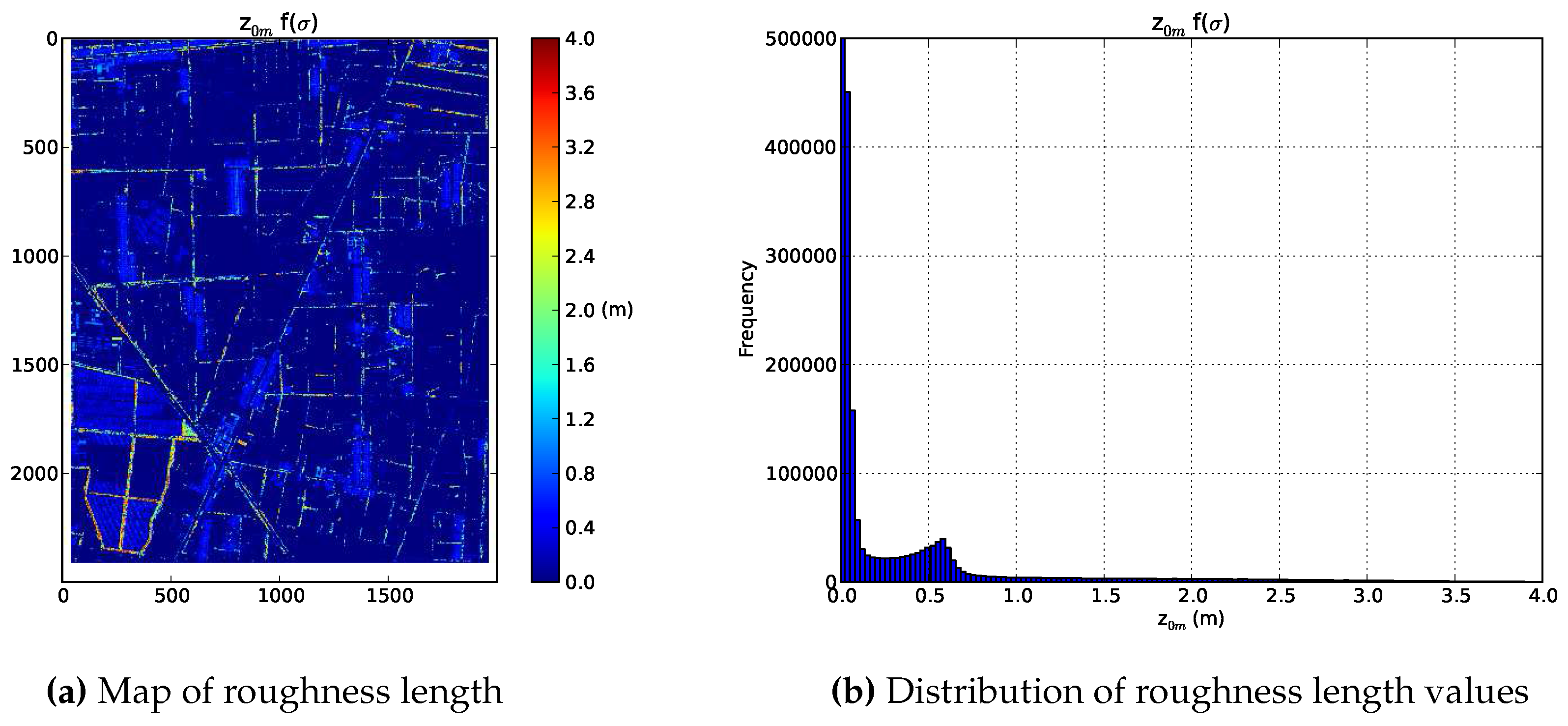
4.2.3. Roughness Length as a Function of the Standard Deviation of Vegetation Height

Another measure of the geometrical regularity of a vegetation canopy is the standard deviation of vegetation height taken as an objective measurement of surface roughness [17,54]. Menenti and Ritchie [17] applied Equation (23) to estimate the local aerodynamics length ( z 0 m ) due to the intervening complete and partial canopies from segments of laser measurements. The original expression proposed by the authors is adapted here for a two-dimensional array, i.e., the digital surface model. Roughness length is derived from the DSM grid using a j by j kernel, where j is an odd number, scanned over all pixels of the grid:
z 0 m = 1 n i = 1 n ( σ h i σ 0 ) h i h ¯
with n = 9 since j = 3 , σ h i the standard deviation of the i- t h pixel of the kernel, σ 0 the instrument noise ( σ 0 = 0.03 ), h i the elevation of the i- t h pixel located inside the kernel and h ¯ the mean elevation in the kernel.
This formulation is the first in a sequence of equations proposed by Menenti and Ritchie [17] to estimate the effective aerodynamic roughness length of a composite landscape. The local z 0 m calculated above is then used to estimate the effective aerodynamic roughness of the mixture of herbaceous vegetation with taller and sparse shrubs and trees ( Z 0 m ), using the following equation [10]:
l n Z 0 m z 0 m = 4 5 l n h z 0 m + l n 1 λ b h B h × 1 1 m λ C d h λ 2 k 2 l n h z 0 m 2 1 / 2
where k is the Von Karman’s constant, m = ( b / h ) + ( B / h ) + ( L / 2 h ) , b is the base width of shrubs (m), h is the height of shrubs (m), B is the base width of the region with separated airflow behind obstacles (m), λ = h / s , s is the spacing of shrubs (m), and L is the restoration length of the logarithmic profile in the surface layer behind obstacles.
To estimate an effective aerodynamic roughness length ( Z 0 m ) which includes the effects of topography, besides low vegetation and shrubs, the formula given by Taylor [55] has to be applied:
l n Z 0 m Z 0 m = 3.5 a 2 π λ 2 l n λ Z 0 m
with a the amplitude of relief (described as periodic) and λ the wavelength of periodic relief.
The Z 0 m values apply to larger length scales and higher air levels than the Z 0 m values obtained with Equation (24). Considering the local scale and the relatively flat terrain of the Yingke area, this formulation is not appropriated in this study and thus not used.
Figure 5 presents the map and distribution of Z 0 m values obtained with the sequence of Equations (23) and (24). The range and the distribution of roughness values is very similar to the results obtained with Equation (22) (cf. Figure 4). Some very high values are also located in the range 1–5 m.

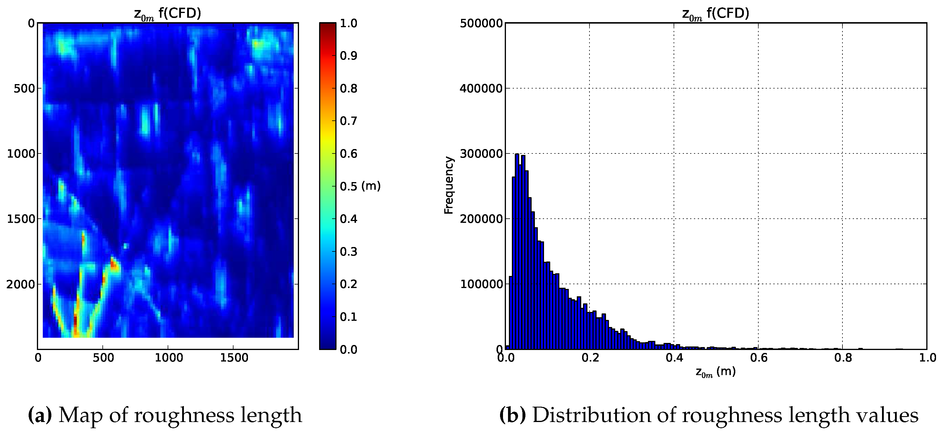
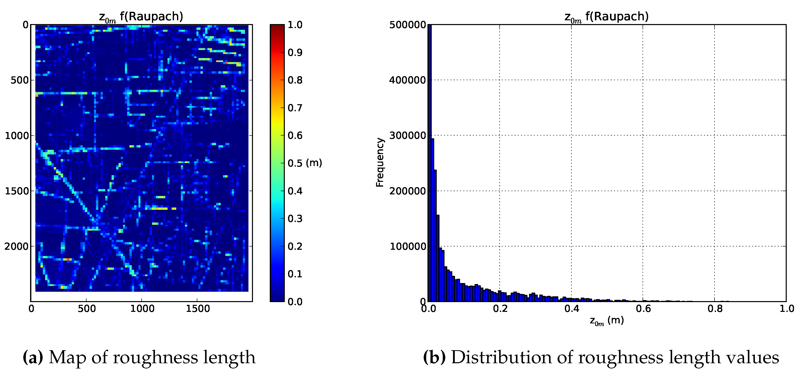
4.2.4. Roughness Length from Raupach’s Formulations and CFD Model

Figure 6 and Figure 7 presents the roughness length values obtained using respectively CFD and Raupach’s models. The two computation were performed with the wind characteristics measured at the Yingke AMS station. The distribution of values retrieved from CFD model is ranging from 0 to 1 m, with a peak around 0.05 m. Lowest values are never equal to 0, since with this method “everything is roughness”. The spatial distribution of roughness values using Raupach’s model is obviously very similar to Brutsaert’s (Figure 4a) and Menenti and Ritchie’s (Figure 5a) methods since they are directly linked to the digital surface model (DSM). Due to the computing resolution, this process provides an aggregation of rough elements. The interesting point is that the range of z 0 m values is more reasonable and consistent with the local landscape.

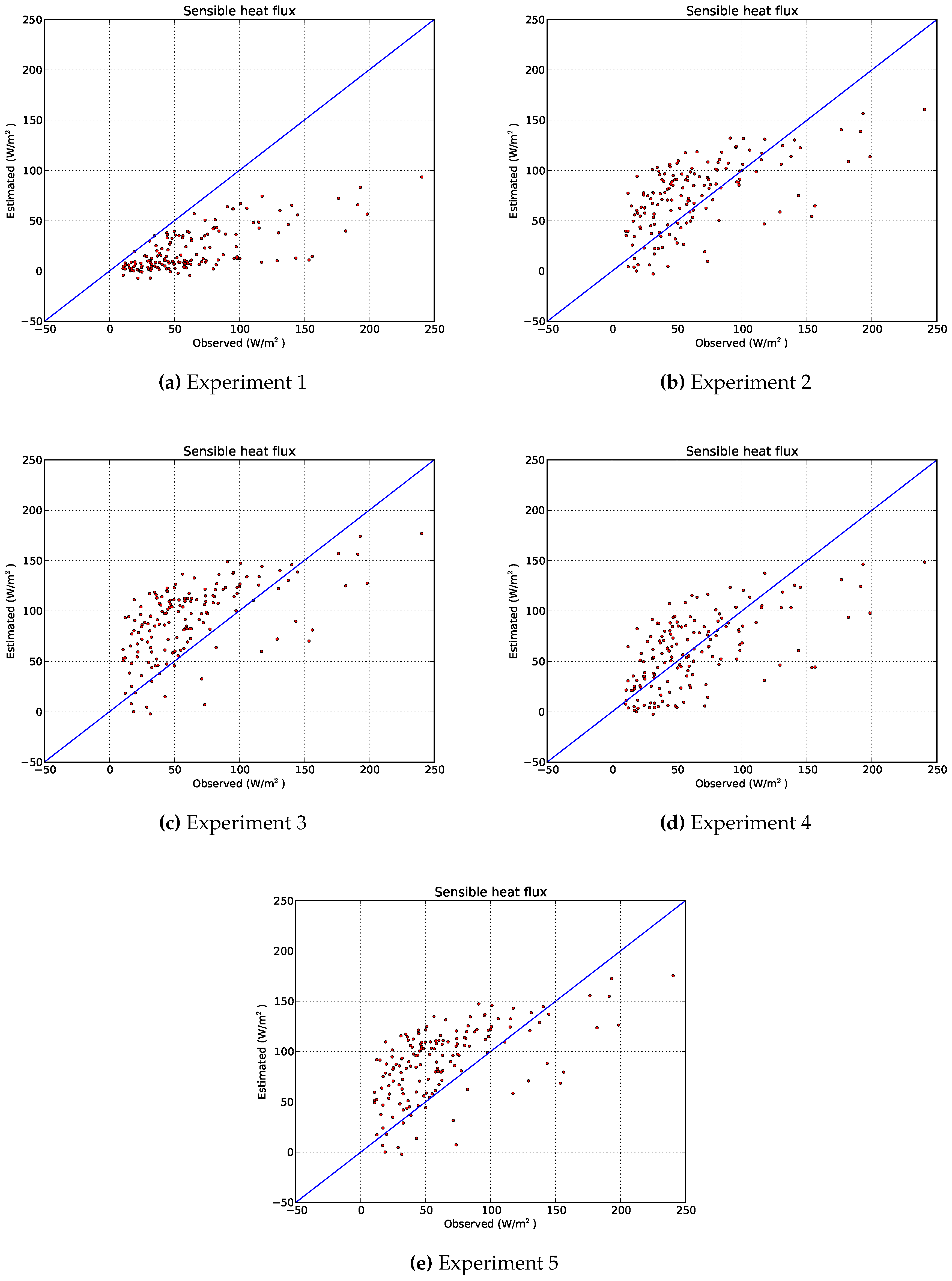
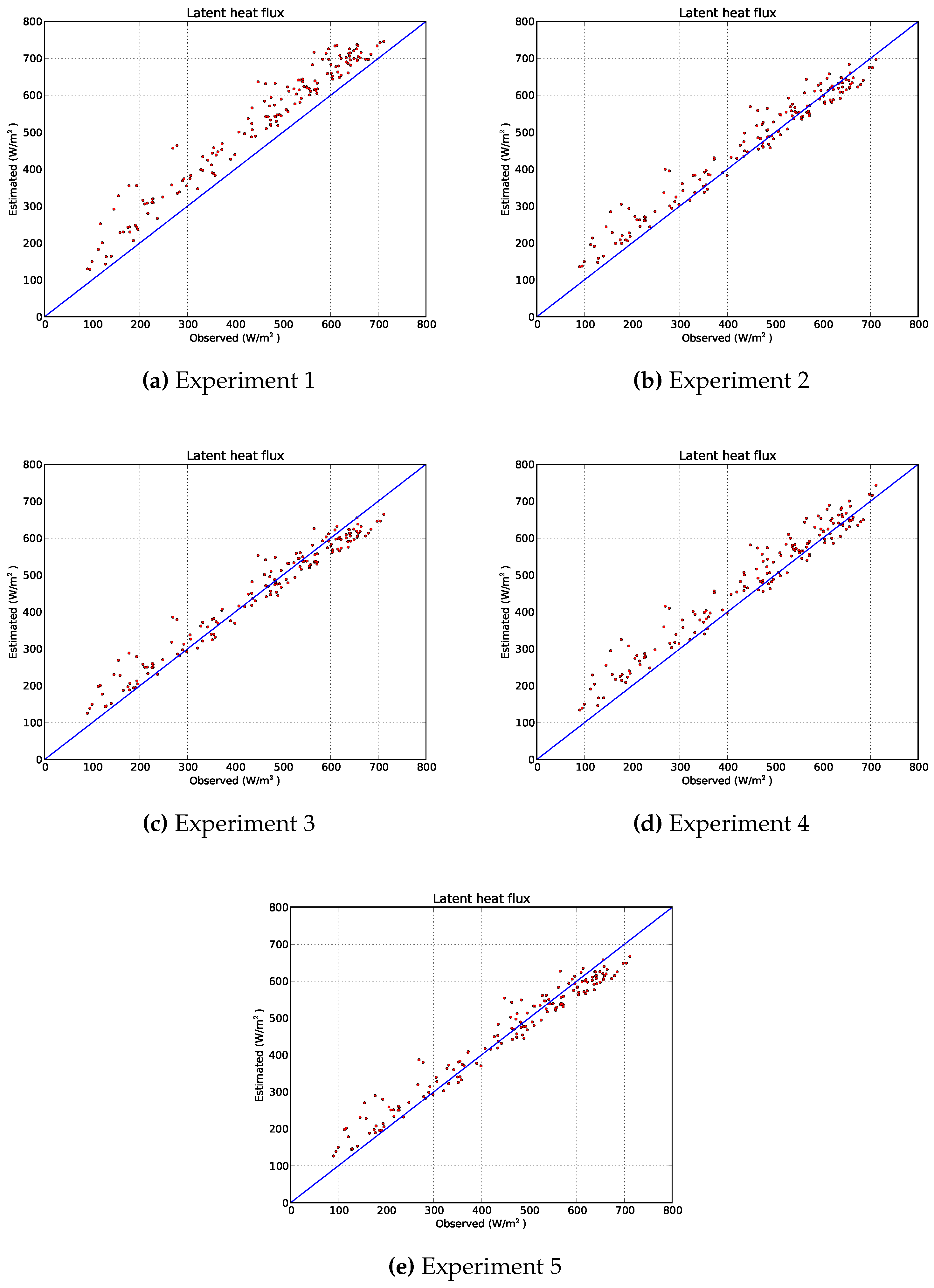
4.2.5. Design of the Different Experiments

Following the different methods proposed for the geometrical characterization of the land surface, a set of five scenarios for surface energy balance estimation is created and results will be compared with ground measurements at the EC footprint scale. Considering the lack of usable WIDAS acquisitions, the evaluation has also to be considered in a temporal perspective. For each numerical experiment, input data are the same but only the vegetation height, zero-plane displacement height and aerodynamic roughness length for momentum are modified. The exact content of the experiments is described below and summarized in Table 1:
-
the first experiment is considered as the ”by default” case for a SEBS calculation, with z 0 m assumed to be function of NDVI, and h v and d 0 to be a fraction of roughness length.
-
the second experiment is a kind of improved ”by default” configuration. The vegetation height is provided by the LIDAR data and d 0 and z 0 m formulations remain the same as before.
-
the third one integrates the effective aerodynamic roughness length retrieved by following Menenti and Ritchie [17]. The vegetation height is provided by the LIDAR data and d 0 is still considered proportional to z 0 m .
-
the fourth one includes z 0 m values retrieved from the inversion of the CFD windfield over the Yingke area. The resolution of roughness data is 25 m, resampled to 1.25 m in order to match with VNIR data. h v is also derived from LIDAR data and d 0 proportional to z 0 m .
-
the last experiment integrates z 0 m and d 0 values computed using Raupach’s formulations. Here again the initial computing resolution is 25 m, resampled to the VNIR data resolution. The vegetation height is provided by the LIDAR data.

5. Spatial Evaluation of Estimated Turbulent Heat Flux Densities at the Footprint Scale

The reliability of geometrical-based and CFD-based roughness retrieval methods proposed by Colin and Faivre [28] is evaluated with their use with the SEBS algorithm. Five experiments are performed in order to compare the benefit of each method presented above in the estimation of turbulent heat fluxes. Atmospheric input data such as longwave and shortwave radiation, wind speed, air temperature, air pressure and specific humidity measured at 10 m above ground level by the AMS are input data applied in all the experiments.

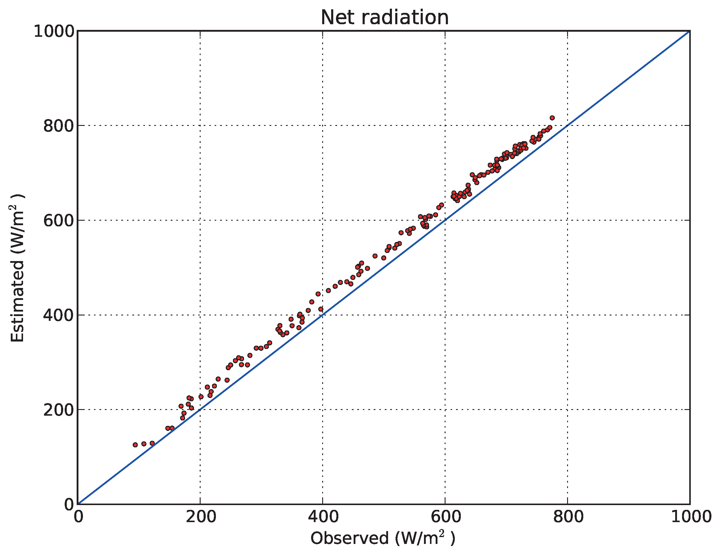
5.1. Surface Radiative Balance

SEBS first resolves surface radiative balance based on WiDAS surface albedo, temperature and emissivity combined with measured incoming longwave and shortwave radiation. Ground heat flux is assumed to be a fraction of net radiation weighted by the fractional vegetation cover (Equation (2)). Surface radiative balance is common for the five experiments since atmospheric and land surface parameters given as input remain the same.
As it is impossible to identify accurately the target seen by the instruments and its corresponding pixel(s), the estimated radiative terms are averaged at the scale of the heat flux footprint. The comparison between measurements and estimates of brightness temperature, ground heat flux and net radiation is given in Table 2.
Net radiation for the source area located upstream of the station is overestimated about 9.7% (+62 W/m 2 ), while brightness temperature is around 1 C less (Table 2). It suggests that the error comes from the estimation of albedo or emissivity. The soil heat flux G 0 is greatly overestimated by SEBS, while the measured value is extremely low considering the surface temperature and the time of measurement (around noon). At this period of the day, considering the season and latitude, the soil heat thermal admittance should be higher. But the estimated at-surface available energy R n G 0 is finally close to measurements with an underestimation of −5.8% (−37 W/m 2 ), since the initial difference is reduced due to a large value of G 0 .

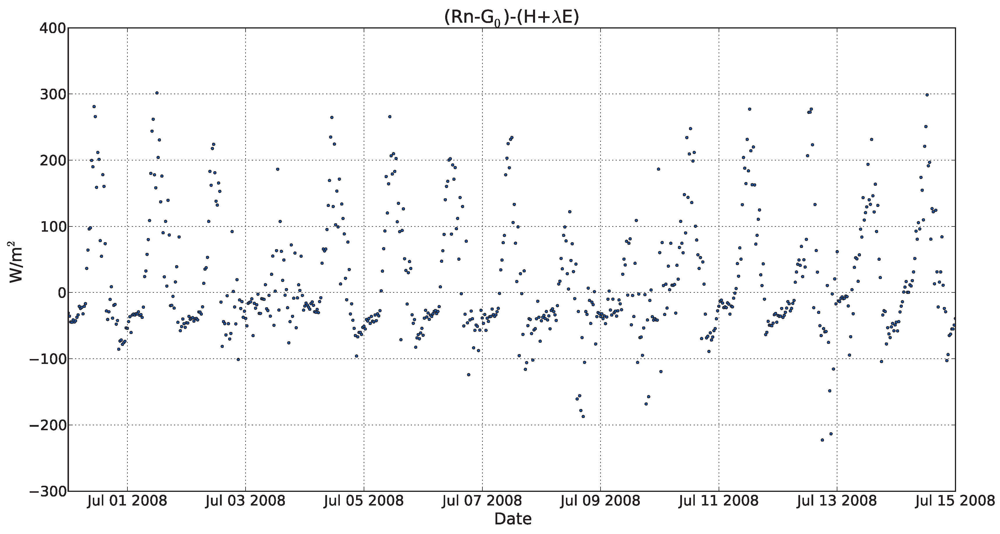
5.2. Surface Energy Balance

Ground measurements of turbulent heat fluxes provided by the eddy covariance system are listed in Table 3. The footprint of the source area of land surface which contributes to the measured heat fluxes has a total area of 17,600 m 2 . Since the measured soil heat flux is very low, the at-surface available energy ( R n G 0 ) is large and exceeds the sum of latent and sensible heat fluxes (+244 W/m 2 ). A method which preserves the Bowen ratio is applied to correct for the unclosed energy balance [56]. The residuum is divided up according the Bowen ratio ( B o = H / λ E ) and distributed to sensible and latent heat accordingly. The Bowen ratio after correction is the same as before.
Heat fluxes are spatially integrated over the source area by applying the footprint weighted coefficients and results are presented in Table 4 for each experiment. Values of spatially integrated roughness lengths and k B 1 are also given. Experiments 2 and 4 are able to estimate H respectively with a difference of +4.9% and −10.6%, λ E of −7.3% and −5.2%, and the partitioning over fluxes is very close to the observed value of evaporative fraction (0.88). It appears clearly that experiment 1, based on Moran [20] for z 0 m retrieval, is the least able to estimate sensible heat fluxes with a large underestimation of about −76.1% since roughness values for momentum and heat transfer are both extremely high for this situation. It confirms the first assessment about the distribution of roughness values in Section 4.2.
Considering not only the strict footprint area, it has to be noticed that there is no result for pixels where z > d 0 , since the negative value of z d 0 returns computing errors in the sequences concerning k B 1 , friction velocity ( u * ), stability functions ( ψ m and ψ h ) and external resistances ( r a h ). It typically occurs where h v is very high in experiments 2 and 3. Also, k B 1 values are consistent in experiments 1 and 2 since they keep proportionality between h v , d 0 and z 0 m . But when d 0 and z 0 m are not directly related to h v as it is the case in experiments 3, 4 and 5, k B 1 values are sometimes huge due to the ratio z 0 m / h v in Equation (8) proposed by Massman [9], which yields calculation errors for some pixels. The consequence is that results of k B 1 and z 0 h in Table 4 are not consistent with z 0 m following the Equation (7).
In experiment 5 this problem is explained by the spatial computing resolution of z 0 m (25 m) which can give high roughness values for pixels where h v is low. Concerning experiment 4, this point is particularly important since the roughness propagates downstream of obstacles following the wind flow, for instance over crops with low vegetation located after high tree rows. A solution could be to set an upper bound on k B 1 , e.g., 25. For experiment 5, this problem could be avoided or reduced by also aggregating h v values. In experiment 4, an other solution could be to remove h v provided by LIDAR data and to use Equation (21) in order to restore proportionality between geometrical terms and to keep consistency in k B 1 values.
Table 5 presents the results for experiments 3, 4 and 5 after modification of the h v values which are now proportional to z 0 m and d 0 as in experiments 1 and 2. This correction does not really affect results of flux densities and related k B 1 and z 0 h in experiments 3 and 5. It means that the deviation in the ratio z 0 m / h v was not so important. However it has a more significant impact in experiment 4 with a sharp decrease of k B 1 from 6.15 to 3.66 and a resulting increase of z 0 h which leads to an underestimation of H (−22.9%) but reduces the error for λ E (−3.6%).
The difference between roughness values is very interesting. For instance, the value estimated with the model proposed by Raupach [29] is very low. According to the Davenport-Wieringa roughness length classification [57,58], this range of values around 0.005 m, corresponds to a ’smooth’ surface, such as a featureless landscape equivalent to a flat beach or snow-covered land. The value of 0.288 m estimated by Moran’s formulation is expected for a ’rough’ surface, as an area with high crops of varying heights and scattered obstacles. This description is not consistent with the station surroundings, but could be consistent with the dense cultivated area located in the south-west part of the scene. The value retrieved from the CFD (0.026 m) is very coherent, according to the same classification it corresponds to an ’open’ surface like low vegetation with isolated obstacles. In this area z 0 m values from CFD are moderate due the absence of huge obstacle and the relative distance from high tree rows. Values retrieved from Brutsaert [38] and Menenti and Ritchie [17] are very similar and in between ’smooth’ and ’open’.
Finally, considering the errors in the estimation of both sensible and latent heat fluxes, and also the ability to preserve the partitioning provided by the evaporative fraction (Λ), experiments 2 and 4 prove to be the most suitable to estimate heat flux densities. However, a validation based on a single case study can not be considered as sufficient and must be repeated several times. Since there is only one WiDAS dataset available over the Yingke area, a temporal evaluation was performed at the scale of the meteorological station.

6. Temporal Evaluation of Estimated Turbulent Heat Flux Densities at the AMS Scale

6.1. Production of a Time-Series

In this section, a short time-series of heat fluxes is produced at the scale of the AMS (one-dimension) in order to perform an evaluation of roughness length retrieval methods based on several occurrences. Considering that the land cover and its associated properties remain slightly constant during few days, the evaluation covers a period of two weeks ranging from the 30 June to the 14 July with a time step of 30 min, for a total of 721 calculations.
Land surface parameters such as albedo, NDVI, LAI, fractional vegetation cover, emissivity, vegetation height and roughness length are averaged over an area corresponding to 100 by 100 pixels (15,000 m 2 ) and centered on the AMS. This subset allows to capture the heterogeneity of the surrounding landscape, but also includes changes in wind direction and the related source area of heat fluxes.
As noticed previously in Section 5, Equation (2) is not really able to estimate accurately soil heat flux in this context. Since the radiative budget is common for all experiments, it is chosen to provide the measured G 0 to SEBS in order to limit errors in the determination of the at-surface available energy R n G 0 . Also, the energy balance is corrected once again using Bowen ratio in order to compensate large differences between R n G 0 and H + λ E as testified in Figure 8.
The correction is only applied when both H and λ E exceed 10 W/m 2 and B o > 0, which limits to 253 the number of occurrences, mainly during daytime. Then, only wind profiles corresponding to near-neutral condition are selected. Stability conditions are estimated using the gradient Richardson number ( R i ):
R i = g T a θ z / u z 2
where θ is the potential temperature. When R i 0 the stratification is neutral and the profile is generally accepted to be logarithmic (Equation (9)). Here the threshold is set to ±0.1, which limits to 161 occurrences for validation. RMSE on estimated R n is 23.4 W/m 2 for the entire period and 32 W/m 2 for the retained cases (Figure 9).

6.2. Results

Table 6 presents RMSE in the estimation of latent and sensible heat fluxes and corresponding roughness length values for each experiment, except experiment 4 for which z 0 m varies following wind measurements. Figure 10 shows the distribution of the 161 roughness length values, with an important frequency in the range 0.025–0.05 m and a secondary peak around 0.1 m. In experiment 5, z 0 m value is considered constant since the variation of wind direction does not induce sensible changes in this context. The scatter plots between measurements and estimations for sensible and latent heat flux are respectively presented in Figure 11 and Figure 12.
This temporal evaluation of estimated heat flux densities reveals that experiments 2 and 4 are the most able to estimate sensible heat flux with respectively RMSE of 33.9 W/m 2 and 30.3 W/m 2 . Experiments 3 and 5 present very close errors since z 0 m values are almost similar. Also, experiment 1 is definitively based on the worst formulation for roughness length retrieval in this context. These results confirm what was observed in Section 5 with the spatial evaluation at the footprint scale.

7. Discussion

This evaluation proves that, in the context of the Yingke oasis station, experiments 2 to 4 gave reliable estimations of sensible heat flux and a consistent partitioning between turbulent heat fluxes, at least in the context of a 1D time-series at the station scale. However, at the footprint scale only experiments 2, 4 and 5 are considered reliable. The absence of other datasets over the Yingke area does not allow to draw rigorous conclusions.
However, results of calculations show that a better estimation of H leads to larger errors on λ E . But, usually the main interest by solving the energy balance in hydrological studies is to obtain a good determination of λ E and, by extension, of the actual evaporation rate. In this sense, experiment 2 gives the smallest errors on H and λ E and keeps the correct partitioning of heat fluxes.
This evaluation also reveals that the estimation of sensible heat flux and partitioning, at the footprint scale, is more consistent in experiment 4 when vegetation height is not corrected with respect to k B 1 . The absence of correction can lead to extreme values of k B 1 in some context and for few pixels, but at the scale of the station it is very appropriate as seen in Table 4. This raises the question about the absolute necessity to keep a linkage between h v , d 0 and z 0 m , whereas the roughness length retrieved from CFD is purely based on an aerodynamic consideration: for a same place, various z 0 m and d 0 values can be observed for a same vegetation shape, since an infinity of wind speed, direction and upstream history are possible.
Linearity between these geometrical parameters ( h v , d 0 and z 0 m ) is always retrieved in the formulations given by Moran or Brutsaert [20,38], or also by Su et al. [18], among others [19,59,60]. Moreover, Su et al. [18] demonstrated that the Massman’s [9] k B 1 model is particularly sensitive to the vegetation height, with a relative error up to 46% of the mean measured H when using 150% of the h v reference value. Thus, if h v is systematically calculated from the retrieved z 0 m values, it increases errors in the parameterization of k B 1 parameter in experiments 3, 4 and 5. This also explain why experiment 2 gives accurate estimates of heat fluxes, since d 0 and z 0 m are derived from the measured h v in a simple and apparently efficient way. It is difficult to determine which is the adequate parameterization for both z 0 m and k B 1 . The use of another k B 1 model, which allows for any roughness length retrieval method, could be relevant.
Also, the representativeness and accuracy of ground measurements should be assessed. The surface energy balance is corrected using the measured radiative budget, but the footprint for SRB and SEB measurements is not the same. There is a considerable difference between the surface covered by the narrow field of view of a pyranometer, and the source area that contributes in EC measurements. Considering an extended homogeneous area (bare soil or fully vegetated), this may not have a large impact. However, this correction is partially biased in a context of heterogeneous landscape such as an irrigated farmland. The meaning of the measured ground heat flux is also a key point. Values of G 0 observed at the Yingke station are very low, and the simple model usually used in SEBS already proved its reliability, but in this context there is a huge deviation. The incapacity to identify the origin of error makes more difficult the correction of measured turbulent heat fluxes using Bowen ratio.

8. Conclusions and Perspectives

The availability of LIDAR data in the framework of the WATER project, has led Colin and Faivre [28] to exploit a Digital Surface Model for estimating roughness length for momentum ( z 0 m ). A pretty new approach developed by the authors consisted in the introduction of the DSM in a CFD model in order to reproduce 3D wind fields, and to invert them for retrieving a spatialized roughness parameter. They also implemented the geometrical Raupach’s approach [29] in the same goal. This study aimed at evaluate these two methods against two empirical ones, widely used in SEBI-based algorithms [20,38], and also against an alternate geometrical model proposed by Menenti and Ritchie [17]. Methods used in experiments 2 (based on Brutsaert [38]) and 4 (based on Colin and Faivre [28]) appear to be the most able to estimate roughness length, according to the estimated heat fluxes, and both at the footprint scale that at the station scale (time-series). However, the formulation used in experiment 2 allows to minimize errors in both latent and sensible heat flux, and to preserve a good partitioning. This formulation is also easier to implement in an operational context. Meanwhile, an additional evaluation of these two methods based on an other k B 1 model is necessary, to avoid the need of proportionality between geometrical terms ( h v > d 0 > z 0 m ) which is not always compatible with CFD-based retrieval method. The methods used in this evaluation are suitable for local studies (except experiment 1), and when LIDAR datasets can be available, which is rather unusual. Considering investigations on roughness length retrieval at larger scales, literature often advocates the use of empirical relationships based on vegetation indices, with all the limitations that were demonstrated here by applying the method from Moran [20]. For regional applications, the likely uncertainty of the roughness information will be significant. For instance, most of the Numerical Weather Prediction Models use a detailed land cover classification combined with phenological data for acting as a surrogate. During the WATER intensive observation period, only one LIDAR acquisition was operated over the Yingke oasis station. In the perspective of an extended study on the seasonality of the land surface roughness, a flight frequency of once every month or two months could be interesting to characterize the annual variation of z 0 m in the Yingke area. The vegetation growth, but also seasonal changes in the regional wind flow, should be key factors in the roughness variation of land surface. Another perspective could be to perform this evaluation again for a place more affected by the surrounding obstacles. In this study, the AMS is located in an open area as it is required for ground measurements. But, considering the investigations for roughness length retrieval, it would be interesting to have a station located downstream to major obstacles, as the area of crops bounded by tree rows on the south-west part of the scene.

Acknowledgments

This work was supported by the ESA Dragon 2 programme under proposal No. 5322: ”Key Eco-Hydrological Parameters Retrieval and Land Data Assimilation System Development in a Typical Inland River Basin of China’s Arid Region” and by the European Commission (Call FP7-ENV-2007-1 Grant No. 212921) as part of the CEOP-AEGIS project (http://www.ceop-aegis.org) coordinated by the University of Strasbourg. WATER was jointly supported by the Chinese Academy of Science Action Plan for West Development Program (grant KZCX2-XB2-09) and Chinese State Key Basic Research Project (grant 2007CB714400).

Author Contributions

Robin Faivre conceived, designed, and performed the experiments, guided and helped in the analyses of the data by Jérôme Colin and Massimo Menenti. Robin Faivre wrote this paper. Robin Faivre and Massimo Menenti reviewed the paper.

Conflicts of Interest

The authors declare no conflict of interest.

References

  1. Li, Z.L.; Tang, R.; Wan, Z.; Bi, Y.; Zhou, C.; Tang, B.; Yan, G.; Zhang, X. A review of current methodologies for regional evapotranspiration estimation from remotely sensed data. Sensors 2009, 9, 3801–3853. [Google Scholar] [CrossRef] [PubMed]
  2. Menenti, M.; Choudhury, B.J. Parameterization of land surface evaporation by means of location dependent potential evaporation and surface temperature range. In Exchange Processes at the Land Surface for a Range of Space and Time Scales, Proceedgins of the Yokohama Symposium; IAHS Publication: Washington, DC, USA, 1993; pp. 561–568. [Google Scholar]
  3. Bastiaanssen, W.; Menenti, M.; Feddes, R.; Holtslag, A.A.M. A remote sensing surface energy balance algorithm for land (SEBAL). 1. Formulation. J. Hydrol. 1998, 212–213, 198–212. [Google Scholar] [CrossRef]
  4. Roerink, G.; Su, Z.; Menenti, M. S-SEBI: A simple remote sensing algorithm to estimate the surface energy balance. Phys. Chem. Earth 2000, 25, 147–157. [Google Scholar] [CrossRef]
  5. Su, Z. The Surface Energy Balance System (SEBS) for estimation of turbulent heat fluxes at scales ranging from a point to a continent. Hydrol. Earth Syst. Sci. 2002, 6, 85–99. [Google Scholar] [CrossRef]
  6. Jia, L.; Li, Z.L.; Menenti, M.; Su, Z.; Verhoef, W.; Wan, Z. A practical algorithm to infer soil and foliage component temperatures from bi-angular ATSR-2 data. Int. J. Remote Sens. 2003, 24, 4739–4760. [Google Scholar] [CrossRef]
  7. Colin, J. Apport de la télédétection optique à la définition d’indicateurs de performance pour l’utilisation de l’eau en agriculture. Ph.D. Thesis, Université Louis Pasteur, Strasbourg, France, 2006. [Google Scholar]
  8. Brutsaert, W. Aspects of bulk atmospheric boundary layer similarity under free-convective conditions. Rev. Geophys. 1999, 37, 439–451. [Google Scholar] [CrossRef]
  9. Massman, W.J. A model study of kBH-1 for vegetated surfaces using localized near-field’ Lagrangian theory. J. Hydrol. 1999, 223, 27–43. [Google Scholar] [CrossRef]
  10. Arya, S.P.S. A drag partition theory for determining the large-scale roughness parameter and wind stress on the Arctic pack ice. J. Geophys. Res. 1975, 80, 3447–3454. [Google Scholar] [CrossRef]
  11. Andreas, E.L. A theory for the scalar roughness and the scalar transfer coefficients over snow and sea ice. Bound.-Layer Meteorol. 1987, 38, 159–184. [Google Scholar] [CrossRef]
  12. Oke, T. Boundary Layer Climates; Routledge Press: New York, NY, USA, 1987. [Google Scholar]
  13. Stull, R. An Introduction to Boundary Layer Meteorology; Kluwer Academic: Dordrecht, The Netherlands, 1999. [Google Scholar]
  14. Garrat, J. The Atmospheric Boundary Layer; Cambridge University Press: Cambridge, UK, 1992; p. 316. [Google Scholar]
  15. Brock, B.W.; Willis, I.C.; Shaw, M.J. Measurements and parameterization of aerodynamic roughness length variations at Haut Glacier d’Arolla, Switzerland. J. Glaciol. 2006, 52, 281–297. [Google Scholar] [CrossRef]
  16. Andreas, E.L. Parameterizing scalar transfer over snow and ice: A review. J. Hydrometeorol. 2002, 3, 417–432. [Google Scholar] [CrossRef]
  17. Menenti, M.; Ritchie, J.C. Estimation of effective aerodynamic roughness of Walnet Gulch watershed with laser altimeter measurements. Water Ressour. Res. 1994, 30, 1329–1337. [Google Scholar] [CrossRef]
  18. Su, Z.; Schmugge, T.; Kustas, W.P.; Massman, W.J. An evaluation of two models for estimation of the roughness height for heat transfer between the land surface and the atmosphere. J. Appl. Meteorol. 2001, 40, 1933–1951. [Google Scholar] [CrossRef]
  19. De Vries, A.C.; Kustas, W.P.; Ritchie, J.C.; Klaassen, W.; Menenti, M.; Rango, A.; Prueger, J.H. Effective aerodynamic roughness estimated from airborne laser altimeter measurements of surface features. Int. J. Remote Sens. 2003, 24, 1545–1558. [Google Scholar] [CrossRef]
  20. Moran, M.S. A Satellite-Based Approach for Evaluation of the Spatial Distribution of Evapotranspiration from Agricultural Lands. Ph.D. Thesis, University of Arizona, Tucson, AZ, USA, 1990. [Google Scholar]
  21. Bastiaanssen, W. Regionalization of Surface Flux Densities and Moisture Indicators Incomposite Terrain: A Remote Sensing Approach under Clear Skies in Mediterranean Climates. Ph.D. Thesis, Wageningen Agricultural University, Wageningen, The Netherlands, 1995. [Google Scholar]
  22. Colin, J.; Menenti, M.; Rubio, E.; Jochum, A. Accuracy vs. operability: A case study over barrax in the context of the idots. In Proceedings of the AIP Conference Proceedings, Naples, Italy, 10–11 November 2005; Volume 852, pp. 75–83.
  23. Ketchum, R.D., Jr. Airborne laser profiling of the arctic pack ice. Remote Sens. Environ. 1971, 2, 41–52. [Google Scholar] [CrossRef]
  24. Hofton, M.A.; Rocchio, L.; Blair, J.; Dubayah, R. Validation of vegetation canopy LIDAR sub-canopy topography measurements for a dense tropical forest. J. Geodyn. 2002, 34, 491–502. [Google Scholar] [CrossRef]
  25. Dorren, L.; Berger, F.; Maier, B. Mapping the structure of forestal vegetation with an airborne light detection and ranging (LIDAR) system in mountainous terrain [Cartographier la structure de la vegetation forestiere avec un systeme LiDAR aeroporte en terrain montagnard]. Rev. Fr. Photogramm. Teledetec. 2007, 186, 54–59. [Google Scholar]
  26. Wang, C.; Menenti, M.; Stoll, M.P.; Feola, A.; Belluco, E.; Marani, M. Separation of ground and low vegetation signatures in LIDAR measurements of salt-marsh environments. IEEE Trans. Geosci. Remote Sens. 2009, 47, 2014–2023. [Google Scholar] [CrossRef]
  27. Streutker, D.R.; Glenn, N. LIDAR measurement of sagebrush steppe vegetation heights. Remote Sens. Environ. 2006, 102, 135–145. [Google Scholar] [CrossRef]
  28. Colin, J.; Faivre, R. Aerodynamic roughness length estimation from very high-resolution imaging LIDAR observations over the Heihe basin in China. Hydrol. Earth Syst. Sci. 2010, 14, 2661–2669. [Google Scholar] [CrossRef]
  29. Raupach, M.R. Simplified expressions for vegetation roughness length and zero-plane displacement as functions of canopy height and area index. Bound.-Layer Meteorol. 1994, 71, 211–216. [Google Scholar] [CrossRef]
  30. MacDonald, R.W.; Griffiths, R.F.; Hall, D.J. An improved method for the estimation of surface roughness of obstacle arrays. Atmos. Environ. 1998, 32, 1857–1864. [Google Scholar] [CrossRef]
  31. Choudhury, B.J.; Idso, S.B.; Reginato, R.J. Analysis of an empirical model for soil heat flux under a growing wheat crop for estimating evaporation by an infrared-temperature based energy balance equation. Agric. For. Meteorol. 1987, 39, 283–297. [Google Scholar] [CrossRef]
  32. Bastiaanssen, W.; Bandara, K. Evaporative depletion assessments for irrigated watersheds in Sri Lanka. Irrig. Sci. 2001, 21, 1–15. [Google Scholar]
  33. Murray, T.; Verhoef, A. Moving towards a more mechanistic approach in the determination of soil heat flux from remote measurements. A universal approach to calculate thermal inertia. Agric. For. Meteorol. 2007, 147, 80–87. [Google Scholar] [CrossRef]
  34. Monteith, J.L.; Unsworth, M.H. Principles of Environmental Physics; Edward Arnold Press: London, UK, 1973. [Google Scholar]
  35. Kustas, W.P.; Daughtry, C.S.T. Estimation of the soil heat flux/net radiation ratio from spectral data. Agric. For. Meteorol. 1989, 49, 205–223. [Google Scholar] [CrossRef]
  36. Chamberlain, A.C. Transport of gases to and from grass and grass-like surfaces. Proc. R. Soc. Lond. 1966, A290, 236–265. [Google Scholar] [CrossRef]
  37. Owen, P.R.; Thomson, W.R. Heat transfer across rough surfaces. J. Fluid Mech. 1968, 15, 321–324. [Google Scholar] [CrossRef]
  38. Brutsaert, W. Evaporation Into the Atmosphere; Kluwer Academic: Dordrecht, The Netherlands, 1982. [Google Scholar]
  39. Counehan, J. Wind tunnel determination of the roughness length as a function of the fetch and the roughness density of three-dimensional roughness elements. Atmos. Environ. (1967) 1971, 5, 637–642. [Google Scholar] [CrossRef]
  40. Wooding, R.A.; Bradley, E.; Marshall, J. Drag due to regular arrays of roughness elements of varying geometry. Bound.-Layer Meteorol. 1973, 5, 285–308. [Google Scholar] [CrossRef]
  41. Lettau, H. Note on aerodynamic roughness-parameter estimation on the basis of roughness-element description. J. Appl. Meteorol. 1969, 8, 828–832. [Google Scholar] [CrossRef]
  42. Theurer, W. Dispersion of Ground-Level Emissions in Complex Built-Up Areas. Ph.D. Thesis, Department of Architecture, University of Karlsruhe, Karlsruhe, Germany, 1993. [Google Scholar]
  43. Lopes, A.M.G. Windstation—A software for the simulation of atmospheric flows over complex topography. Environ. Model. Softw. 2003, 18, 81–96. [Google Scholar] [CrossRef]
  44. Li, X.; Li, X.I.; Li, Z.; Ma, M.; Wang, J.; Xiao, Q.; Liu, Q.; Che, T.; Chen, E.; Yan, G.; et al. Watershed allied telemetry experimental research. J. Geophys. Res. D Atmos. 2009, 114. [Google Scholar] [CrossRef]
  45. Li, F.; Qiang, L.; Qing, X.; Qinhuo, L.; Zhigang, L. Design and Implementation of Airborne Wide-Angle Infrared Dual-mode Line/area Array Scanner in Heihe Experiment. Adv. Earth Sci. 2009, 24, 696–705. [Google Scholar]
  46. Schuepp, P.; Leclerc, M.; Macpherson, J. Footprint prediction of scalar fluxes from analytical solutions of the diffusion equation. Bound.-Layer Meteorol. 1990, 50, 353–373. [Google Scholar] [CrossRef]
  47. Colin, J.; Roupioz, L.; Ghafarian, H.; Bai, J.; Jia, L.; Liu, S.; Faivre, R.; Nerry, F.; Menenti, M. Surface Radiative and Energy Balance Time-Series Processing and Validation Procedure Document; Technical Report, CEOP-AEGIS Deliverable Report De3.3; University of Strasbourg: Strasbourg, France, 2011; p. 34. [Google Scholar]
  48. Su, Z. Remote Sensing Applied to Hydrology: The Sauer River Basin Study. Ph.D. Thesis, Wageningen University and Research, Wageningen, The Netherlands, 1996. [Google Scholar]
  49. Zheng, G.; Moskal, M. Retrieving Leaf Area Index (LAI) using remote sensing: Theories, methods and sensors. Sensors 2009, 9, 2719–2745. [Google Scholar] [CrossRef] [PubMed]
  50. Carlson, T.N.; Ripley, D.A. On the relation between NDVI, fractional vegetation cover, and leaf area index. Remote Sens. Environ. 1997, 62, 241–252. [Google Scholar] [CrossRef]
  51. Baret, F.; Clevers, J.; Steven, M. The robustness of canopy gap fraction estimates from red and near-infrared reflectances: A comparison of approaches. Remote Sens. Environ. 1995, 54, 141–151. [Google Scholar] [CrossRef]
  52. Wittich, K.P.; Hansing, O. Area-averaged vegetative cover fraction estimated from satellite data. Int. J. Biometeorol. 1995, 38, 209–215. [Google Scholar] [CrossRef]
  53. De Griend, A.A.V.; Owe, M. On the relationship between thermal emissivity and the normalized difference vegetation index for natural surfaces. Int. J. Remote Sens. 1993, 14, 1119–1131. [Google Scholar] [CrossRef]
  54. Menenti, M.; Ritchie, J.C.; Humes, K.S.; Parry, R.; Pachepsky, Y.; Gimenez, D.; Leguizamon, S. Estimation of aerodynamic roughness at various spatial scales. John Wiley & Sons: Chichester, UK, 1996. [Google Scholar]
  55. Taylor, P.A.; Sykes, R.I.; Mason, P.J. On the parameterization of drag over small-scale topography in neutrally-stratified boundary-layer flow. Bound.-Layer Meteorol. 1989, 48, 409–422. [Google Scholar] [CrossRef]
  56. Twine, T.E.; Kustas, W.P.; Norman, J.M.; Cook, D.R.; Houser, P.R.; Meyers, T.P.; Prueger, J.H.; Starks, P.J.; Wesley, M.L. Correcting eddy-covariance flux underestimates over a grassland. Agric. For. Meteorol. 2000, 103, 279–300. [Google Scholar] [CrossRef]
  57. Wieringa, J. How far can agrometeorological station observations be considered representative? In Proceedings of the 23rd Conference on Agriculture and Forest Meteorology, Boston, MA, USA, 2–6 November 1998.
  58. Wieringa, J.; Davenport, A.G.; Grimmond, C.S.B.; Oke, T.R. New revision of Davenport roughness classification. In Proceedings of the 3rd European and African Conference on Wind Engineering, Eindovhen, The Netherlands, 2–6 July 2001.
  59. Covey, W. A Method for the Computation of Logarithmic Wind Profile Parameters and Their Standard Errors; Chapter The Energy Budget at the Surface, Part II, Report No. 72; USDA-ARS: Washington, DC, USA, 1963; pp. 28–33.
  60. Kustas, W.P.; Choudhury, B.J.; Kunkel, K.E.; Gay, L.W. Estimate of the aerodynamic roughness parameters over an incomplete canopy cover of cotton. Agric. For. Meteorol. 1989, 46, 91–105. [Google Scholar] [CrossRef]
Figure 1. (a,b) Location map of the Heihe river basin in China. (c) Footprint of the WiDAS and LIDAR acquisition in the Yingke oasis experimental area, where the station is located.
Remotesensing 09 00063 g001
Figure 2. Example of 3-D rendering of the South-West part of the Yingke area obtained by combination of the LIDAR Digital Surface Model and the high resolution image simultaneously acquired by the CCD camera installed together with the LiteMapper 5600.
Remotesensing 09 00063 g002
Figure 3. (a) Map and (b) frequency distribution of roughness length for momentum transfer values over the Yingke oasis station following Moran’s formulation.
Remotesensing 09 00063 g003
Figure 4. (a) Map and (b) frequency distribution of roughness length for momentum transfer values over the Yingke oasis station following Brutsaert’s formulation.
Remotesensing 09 00063 g004
Figure 5. (a) Map and (b) frequency distribution of roughness length for momentum transfer values over the Yingke oasis station retrieved from σ h .
Remotesensing 09 00063 g005
Figure 6. (a) Map and (b) frequency distribution of roughness length for momentum transfer values over the Yingke oasis station retrieved from CFD model.
Remotesensing 09 00063 g006
Figure 7. (a) Map and (b) frequency distribution of roughness length for momentum transfer values over the Yingke oasis station retrieved from Raupach’s model.
Remotesensing 09 00063 g007
Figure 8. Time-series of energy balance deficit from the 30 June to the 14 July 2008 at the Yingke station.
Remotesensing 09 00063 g008
Figure 9. Scatter plot of measured and estimated net radiation from the 30 June to the 14 July 2008 at the Yingke station. RMSE = 32 W/m 2 .
Remotesensing 09 00063 g009
Figure 10. Distribution of z 0 m values retrieved from wind profiles measured at the AMS (mean: 0.13 m, std dev.: 0.20 m).
Remotesensing 09 00063 g010
Figure 11. Scatter plots of measured and estimated sensible heat flux for (a) experiment 1, (b) experiment 2, (c) experiment 3, (d) experiment 4, (e) experiment 5.
Remotesensing 09 00063 g011
Figure 12. Scatter plots of measured and estimated latent heat flux for (a) experiment 1, (b) experiment 2, (c) experiment 3, (d) experiment 4, (e) experiment 5.
Remotesensing 09 00063 g012
Table 1. Summary of methods used for the surface geometrical characterization in each experiment performed over the Yinke area.
METHODS
Experiment No.NDVILIDARM&RCFDRaupach
1 . h v - z 0 m - d 0
2 . h v - z 0 m - d 0
3 . h v z 0 m - d 0
4 . h v z 0 m - d 0
5 . h v z 0 m - d 0
Table 2. Measurements of radiative terms at the Yingke station for the 7 July 2008 at 11:30 a.m. (Beijing time).
VariablesMeasuredEstimated
R n (W/m 2 )637.4699.4
G 0 (W/m 2 )9.0107.5
R n G 0 (W/m 2 )628.4591.9
T b ( C)26.525.4
Table 3. Measured and corrected heat flux densities at the Yingke station for the 7 July 2008 at 11:30 a.m. (Beijing time).
VariablesMeasuredCorrectedVariation
λ E (W/m 2 )340.1556.1+216.0
H (W/m 2 )44.272.3+28.1
Λ (-)0.880.88
Table 4. Results of simulated heat flux densities and roughness length at the EC footprint scale for the five experiments.
Experiment No. λ E HΛ z 0 m kB 1 z 0 h
(W/m 2 )(W/m 2 )(-)(m)(-)(m)
1.589.918.10.970.2883.850.0058
2.512.079.70.870.0143.590.0004
3.467.7124.10.790.0173.490.0001
4.523.767.80.890.0266.150.0005
5.500.791.20.850.0083.990.0001
Table 5. Results of simulated heat fluxes densities and roughness length at the EC footprint scale after k B 1 correction.
Experiment No. λ E HΛ z 0 m kB 1 z 0 h
(W/m 2 )(W/m 2 )(-)(m)(-)(m)
3.466.6123.70.790.0173.390.0001
4.532.258.60.900.0263.660.0007
5.502.389.60.850.0083.560.0003
Table 6. RMSE of simulated heat flux densities and associated roughness length at the AMS scale.
Experiment No. λ E (W/m 2 )H (W/m 2 )Λ (-) z 0 m (m)
1.76.247.10.1140.2535
2.35.733.90.0760.0128
3.33.745.00.0840.0027
4.44.830.30.081-
5.33.543.90.0840.0032

