Distinguishing Intensity Levels of Grassland Fertilization Using Vegetation Indices

Abstract

Monitoring the reaction of grassland canopies on fertilizer application is of major importance to enable a well-adjusted management supporting a sustainable production of the grass crop. Up to date, grassland managers estimate the nutrient status and growth dynamics of grasslands by costly and time-consuming field surveys, which only provide low temporal and spatial data density. Grassland mapping using remotely-sensed Vegetation Indices (VIs) has the potential to contribute to solving these problems. In this study, we explored the potential of VIs for distinguishing five differently-fertilized grassland communities. Therefore, we collected spectral signatures of these communities in a long-term fertilization experiment (since 1941) in Germany throughout the growing seasons 2012–2014. Fifteen VIs were calculated and their seasonal developments investigated. Welch tests revealed that the accuracy of VIs for distinguishing these grassland communities varies throughout the growing season. Thus, the selection of the most promising single VI for grassland mapping was dependent on the date of the spectra acquisition. A random forests classification using all calculated VIs reduced variations in classification accuracy within the growing season and provided a higher overall precision of classification. Thus, we recommend a careful selection of VIs for grassland mapping or the utilization of temporally-stable methods, i.e., including a set of VIs in the random forests algorithm.

1. Introduction

Grasslands are the largest of the Earth’s four major vegetation types and belong to the world’s most productive agricultural lands [1]. Grass swards are known for their high spatial and temporal variability [2] and therefore require intensive monitoring to enable a management that is well adjusted to the prevailing environmental conditions. Maps displaying the phenological status of grassland allow creating a spatio-temporal model of grassland production [3]. Such information is crucial for adjusting the nutrient management in order to mitigate water pollution (through leaching of soil nutrients) and to conserve the flora and fauna of grassland ecosystems. Commonly, grassland agronomists evaluate the phenological status, the quality and the spatial distribution of grasslands in costly and time-consuming field surveys, as described in Cornelissen et al. [4]. The methods defined in this handbook require destructive sampling and allow only a low spatial and temporal data density. Research developing non-destructive, cost-effective and time-saving methods for grassland mapping and monitoring is urgently needed. These goals can be reached using a combination of minor field sampling efforts and remote sensing [5].

Among remote sensing methods, Vegetation Indices (VIs) are frequently used for assessing different grasslands types (e.g., [5,6]). Classification of these types based on VIs requires consideration of the timing of data acquisition in relation to growth stage, as well as of type, wavelength and bandwidth of the VI used. Aragón and Oesterheld [5,7] have shown that classification accuracy of grasslands depends on the date of the spectral observation. The reason for these changes in classification accuracy is that the optical properties of grassland vegetation are underlying permanent variations [8].

These variations in the individual VIs throughout a growing season are caused by changes in the vegetation’s biophysical properties as a result of climatic conditions in interaction with management actions [9]. VIs composed of near-infrared and visible light strongly correlate with biomass [10], LAI and chlorophyll content [11,12]. Thus, VIs based on these wavelengths are capable of distinguishing vegetation canopies, as long as they differ significantly in these variables. In contrast, spectral reflectance at longer wavelengths (between 1300 and 2500 nm) is highly influenced by water absorption of plants [13,14]. This relation between plant water content and absorption of incoming radiation affects the spectral reflectance of plants. Thus, selecting VIs sensitive to the vegetation’s water content may enable a successful classification at times when those VIs appear relatively similar, which are sensitive to other crop variables, such as biomass, leaf area index or chlorophyll content. Further, VIs more sensitive to nitrogen and lignin content, as well as to morphological and physiological properties indicating plant stress may improve classifications at times when grasslands differ in these variables.

Furthermore, bandwidth and spectral resolution have a major impact on the ability of VIs to distinguish grassland communities. Although several efforts have been made to classify grasslands using broadband data [15,16,17], it was found that they are not spectrally distinct in the broadband system throughout all times of a growing season [18]. Numata et al. [18] have shown that the utilization of hyperspectral data may significantly improve the quality of maps displaying the distribution of different grassland communities. Novel or planned hyperspectral satellite missions (such as Hyperion, EnMAP and Hyperspectral Infrared Imager—HyspIRI) may open new perspectives for mapping grasslands using narrowband VIs and are of special importance for distinguishing grassland types and management characteristics, as well as for monitoring these plant communities [1].

Hyperspectral RS can provide a cost-effective, time-saving and non-destructive method for mapping differences in growth dynamics as induced by fertilizer application, as well as the spatial distribution of grassland communities at high spatial and temporal resolution. However, multitemporal studies investigating the performance of hyperspectral and broadband VIs for mapping Central-European grasslands are still missing. Basic research into this direction necessitates not only a high temporal, but also a high spatial and spectral resolution of remote sensing data across clearly-defined grassland communities. These requirements are not met using satellite data only, because frequent cloud cover and low spatial coverage of hyperspectral satellite systems prevents acquiring dense time series in Central Europe. The solution lies in utilizing field spectrometers, which can acquire hyperspectral data on demand for dates when cloud cover is low. To collect spectra of clearly separable grassland communities, we identified a fertilizer experiment on grassland as the ideal setting.

The above-mentioned deficits in the classification of grassland types make clear that studies are required where the criteria growth stage, bandwidth and type of VI are rigorously tested. Therefore, the aim of this study was to identify single VIs providing the most valuable information at specific points in time that enable grassland scientists to distinguish between differently-managed grassland communities. Furthermore, we introduce a novel approach in grassland research, which uses multiple VIs sensitive to changes in different plant properties for classifying grasslands. Accordingly, our key hypotheses were:

• Each plant community on grassland is characterized by a unique VI development throughout the growing season.
• The performance of each VI for distinguishing such plant communities varies throughout the growing season.
• VIs sensitive to a certain plant property (e.g., chlorophyll content) may allow a successful classification at times when VIs sensitive to other plant properties (e.g., water content, biomass, etc.) fail to classify correctly.
• Combining several VIs for grassland classification allows a temporally more stable classification of grassland communities than one single VI because for distinguishing communities at a point in time, a set of optimal VIs is selected.

To test these hypotheses, we collected a series of spectral signatures of five species-rich grassland communities in a long-term fertilization experiment for 38 dates during the growing seasons of 2012–2014. Subsequently, we calculated fifteen broadband and narrowband VIs and tested the performance of each single VI for distinguishing these five communities using the Welch test [19]. In addition, we tested multiple VIs for classifying the same grassland communities using the random forests algorithm [20]. Finally, we compared the classification accuracy achieved using single VIs and the Welch test to the performance reached by the random forests algorithm.

2. Materials and Methods

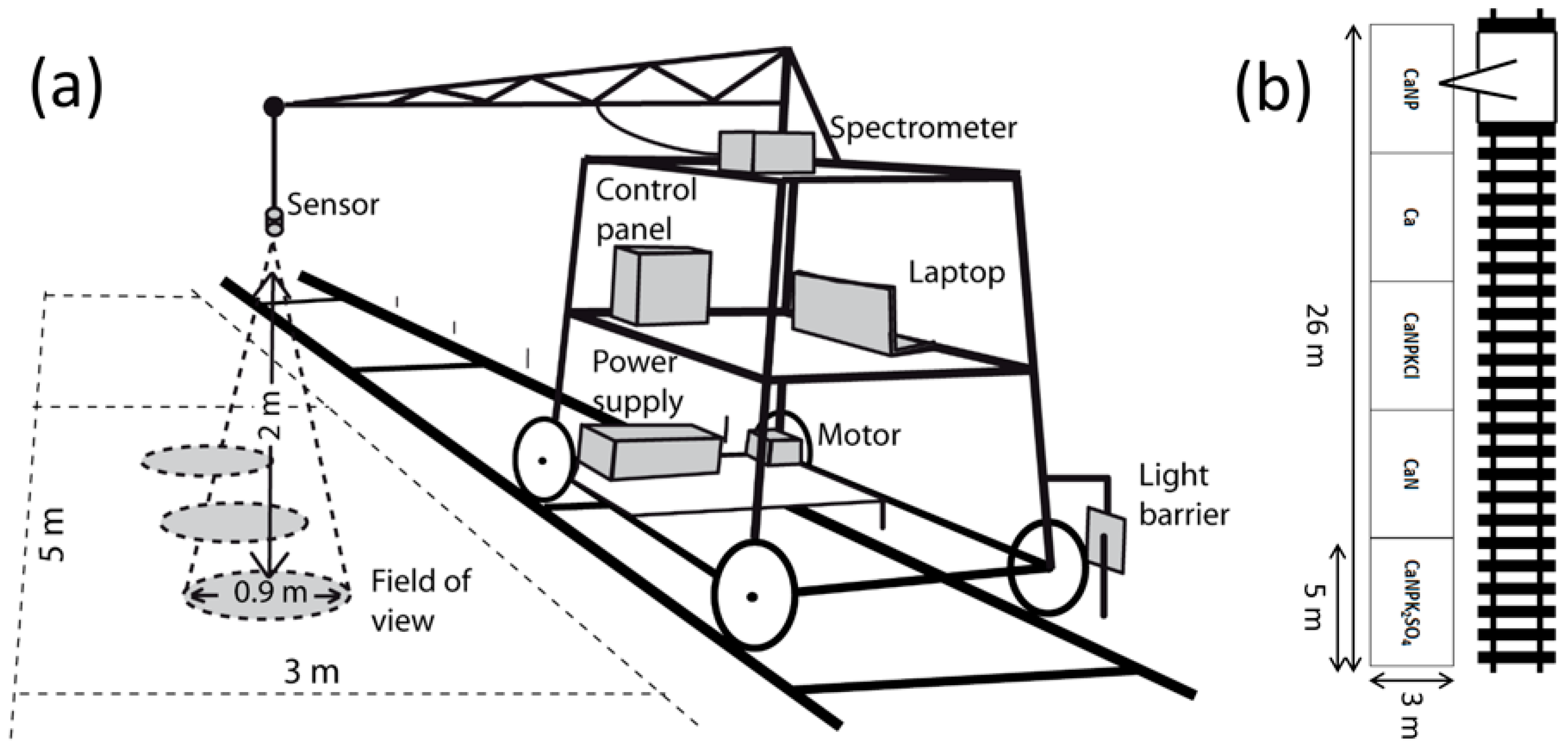
2.1. Study Area

The Rengen Grassland Experiment (RGE) is a long-term fertilization experiment, which was set up in 1941. It is located near the village of Rengen (Rhineland-Palatinate, Germany) in the Eifel Mountains, approximately 60 km west of Koblenz. The experiment is located at the position 50°14′21.6″N, 6°49′34.6″E at an elevation of 475 m asl. The temperate, maritime climate at the site features an annual mean precipitation of 811 mm and a mean annual temperature of 6.9 °C (Rengen Experiment Meteorological Station). A detailed description of the experiment is given in Schellberg et al. 1999 [21]. In brief, the experiment was set up on a formerly wet heathland site in randomized block design. In 1941, the area was grubbed, and a mixture of grasses and herbs was sown. Five fertilizer treatments have been applied annually: lime only as calcium oxide (CaO, Ca), lime and nitrogen (CaO/N, CaN), lime, nitrogen and phosphorous (CaO/N/P₂O₅, CaNP) and lime, nitrogen and potassium (CaO/N/P₂O₅/KCl, CaNPKCl and CaO/N/P₂O₅/K₂SO₄, CaNPK₂SO₄, respectively). The plots in this experiment are representative of grassland fields on farms under different management intensities and stand for fields of a similar type spread all across European grassland areas. Treating the plots with different types of fertilizer resulted in significant differences in plant and soil nutrient content (for more details, see [22]).

This work was conducted on five plots of the RGE with a size of 3 m × 5 m (Figure 1). The plots were harvested twice annually, i.e., once at the beginning of July and once in the middle of October. Previously-published data from this experiment [21,23] indicate that dry matter production increased gradually from Ca, CaN, CaNP, CaNPK₂SO₄ to the CaNPKCl treatment and that biomass production in the first cut was higher than in the second cut. Furthermore, long-term fertilization resulted in significant differences in the floristic compositions of the communities. The vegetation in the Ca and CaN treatments mostly resemble the montane meadow of Geranio-Trisetetum (Polygono-Trisetion), whereas the CaNP plot features a transitional type between Poo-Trisetetum and Arrhenateretum (both from the Arrhenatherion alliance) [24]. In the NPK treatments, vegetation corresponded to the mesotrophic Arrhenateretum meadows [24].

All of these differences in the properties of plant canopies have strong effects on their optical characteristics. Generally, a more rapid change in visual appearance at the beginning of the growing seasons is observed in the NPK-treated plots each year. These plots develop rapidly in green biomass and reach high LAIs and a bright green canopy. Later, in June, senescence of plants commences, which leads to higher contributions of senesced yellow plant material. In contrast, development in green biomass in the Ca and CaN treatment is usually much slower, but the color of these canopies remains green, even later in the growing season.

2.2. Spectral Measurements

Field spectrometers have successfully been used for discriminating differences in grassland types caused by management practices or climatic variability [1,8]. In addition, there is evidence in the literature that field spectrometer data are highly correlated with satellite data [9] and relatively free of atmospheric effects [25]. Thus, we collected spectral measurements in the RGE during the growing seasons of 2012–2014 (

Table 1. Number of data acquisition days between 2012 and 2014.

	No. of Acquisition Days
	2012	2013	2014
1st growth	4	7	8
2nd growth	7	6	6

) using an ASD Fieldspec^® 3 spectroradiometer (Analytical Spectral Devices, Boulder, CO, USA). This instrument covers a spectral range between 350 nm and 2500 nm in 1-nm steps, with a 3-nm full width at half maximum (FWHM) at a wavelength of 700 nm and 10 nm at 1400 nm and 2100 nm (ASD Inc. 2010).

The spectrometer was mounted on a motor-driven rail-crane that automatically moved along a rail track next to the five plots. It was equipped with a photoelectric guard (light barrier) to ensure a systematic sampling of spectral properties at the same position (Figure 1; cf. [26]). From this vehicle, spectra of the vegetation were measured on three circular spots within each plot from a height of 2 m above ground at nadir position, resulting in a Field Of View (FOV) of 90 cm in diameter per spot (Figure 1). On each measuring day, between twelve and thirty-three spectra per plot were acquired between 10:00 a.m. and 4:00 p.m., i.e., between 210 min before and 150 min after solar noon. Spectra were recorded under clear (sunny) conditions, which ensured that influences of clouds were minimal. The spectral reflectance of the plant canopies was calculated based on a Spectralon^® 400-cm² white-reference zenith polymer target (95% reflectance, Labsphere Inc., North Hutton, NH, USA) always after three measurements were taken.

2.3. Calculation of the Temperature Sum

It is well known that changes in plant development are closely related to changes in weather variables, such as precipitation and accumulated temperature [9,27], and not to the date or day of year. Thus, we decided to use the temperature sum (T∑) as the temporal variable. T∑ was calculated for the years 2012–2014 based on the average daily temperatures given in the 1 × 1 km mosaic, provided by Deutscher Wetterdienst [28] according to the method by Ernst and Loeper [29]. Daily mean temperatures above 0 °C were added up. To correct for low solar irradiation during the winter months, a weight factor of 0.5 was assigned to January, 0.75 to February and 1 to the remaining months [29]. As a starting point of the growing season, a value of 200 °C d was assumed. At this point and before the onset of the second growth in July, T∑ was set to zero to provide equal scales for the first and the second growth.

2.4. Calculation of the VIs

Based on the spectral measurements (Supplement Table S1), 12 narrowband and 3 broadband VIs were calculated (

Table 2. Selected VIs for discriminating differently-fertilized grassland plots.

VI	VI Full Name	Formula	Sensitivity	Source
GNDVI	Green Normalized Difference Vegetation Index	$\frac{\left(\mathrm{NIR}-\mathrm{GREEN}\right)}{\left(\mathrm{NIR}+\mathrm{GREEN}\right)}$	Green vegetation/biomass, LAI	[34]
nGNDVI	narrowband Green Normalize Difference Vegetation Index	$\frac{\left(780\mathrm{nm}-550\mathrm{nm}\right)}{\left(780\mathrm{nm}+550\mathrm{nm}\right)}$	Green vegetation/biomass, LAI	[34]
NDVI	Normalized Difference Vegetation Index	$\frac{\left(\mathrm{NIR}-\mathrm{RED}\right)}{\left(\mathrm{NIR}+\mathrm{RED}\right)}$	Green vegetation/biomass, LAI	[35]
nNDVI	narrowband Normalized Difference Vegetation Index	$\frac{\left(800\mathrm{nm}-670\mathrm{nm}\right)}{\left(800\mathrm{nm}+670\mathrm{nm}\right)}$	Green vegetation/biomass, LAI	[35]
nREP	narrowband Red Edge Position	$700+\frac{40\times \frac{670\mathrm{nm}+780\mathrm{nm}}{2}-700\mathrm{nm}}{740\mathrm{nm}-700\mathrm{nm}}$	Chlorophyll	[36]
LCI	Leaf Chlorophyll Index	$\frac{\left(\mathrm{NIR}-\mathrm{RE}\right)}{\left(\mathrm{NIR}-\mathrm{Red}\right)}$	Chlorophyll	[37]
nLCI	narrowband Leaf Chlorophyll Index	$\frac{\left(850\mathrm{nm}-710\mathrm{nm}\right)}{\left(850\mathrm{nm}+680\mathrm{nm}\right)}$	Chlorophyll	[37]
nNPCI	narrowband Normalized Pigment Chlorophyll Index	$\frac{\left(680\mathrm{nm}-430\mathrm{nm}\right)}{\left(680\mathrm{nm}+430\mathrm{nm}\right)}$	Chlorophyll	[38]
nNDLI	narrowband Normalized Difference Lignin Index	$\frac{\log \frac{1}{1754\mathrm{nm}}-\log \frac{1}{1680\mathrm{nm}}}{\log \frac{1}{1754\mathrm{nm}}+\log \frac{1}{1680\mathrm{nm}}}$	Lignin content	[39]
nNDNI	narrowband Normalized Difference Nitrogen Index	$\frac{\log \frac{1}{1510\mathrm{nm}}-\log \frac{1}{1680\mathrm{nm}}}{\log \frac{1}{1510\mathrm{nm}}+\log \frac{1}{1680\mathrm{nm}}}$	Nitrogen content	[39]
nPRI	narrowband Photochemical Reflectance Index	$\frac{\left(550\mathrm{nm}-530\mathrm{nm}\right)}{\left(550\mathrm{nm}+530\mathrm{nm}\right)}$	Physiology (photosynthesis, pigments)	[38]
nWC	narrowband Water Content	$\frac{1193\mathrm{nm}}{1126\mathrm{nm}}$	Water content/water stress	[40]
nWI	narrowband Water Index	$\frac{900\mathrm{nm}}{970\mathrm{nm}}$	Water content	[41]
nSIPI	narrowband Structure Intensive Pigment Index	$\frac{\left(800\mathrm{nm}-450\mathrm{nm}\right)}{\left(800\mathrm{nm}+650\mathrm{nm}\right)}$	Pigments	[42]
nNPQI	narrowband Normalized Phaeophytization Index	$\frac{\left(415\mathrm{nm}-435\mathrm{nm}\right)}{\left(415\mathrm{nm}+435\mathrm{nm}\right)}$	Phaeophytization	[43]

). For calculating the broadband VIs, five bands of the multispectral RapidEye satellites were simulated using their spectral response function ([30]; Supplement Table S2):

$${\gamma }_x=\frac{{{\displaystyle \int }}_{n0}^n{\gamma }_n*{\rho }_n}{{\rho }_t}$$

(1)

where γ_x is the reflectance of the simulated RapidEye band, n is the band number of the spectral measurement, γ_n is the reflectance of band n, ${\rho }_n$ is the response of band n, given in the spectral response function, and ${\rho }_t$ is the sum of values given in a response function of band x. RapidEye appeared for us as an interesting broadband sensor because its spatial resolution (6.5 m) is higher than that of other broadband systems (e.g., Landsat 7, 8 or Sentinel 2) and was thus better comparable to the high spatial resolution of field spectrometer data. We selected these VIs because they are sensitive to different plant properties, contained different spectral information and are commonly used in grassland science. The VIs that were used can be grouped into three categories according to Table 2:

• VIs sensitive to green vegetation, biomass and leaf area,
• VIs sensitive to plant chlorophyll content,
• VIs sensitive to the plants’ content in lignin, nitrogen, water, pigments or to plant physiological performance and phaeophytization (environmental stress).

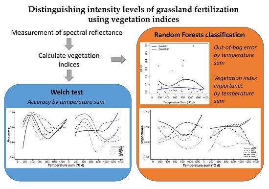
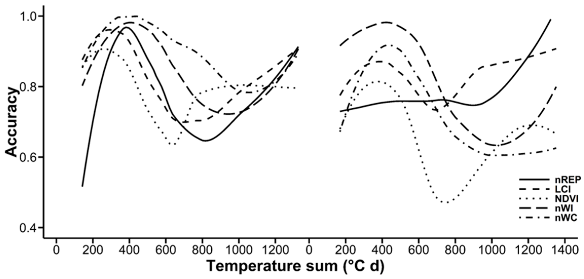
To display the temporal development of the VIs as smoothed curves, first daily averages for each VI were calculated. Subsequently, the local polynomial smoothing algorithm (loess) [31], which is implemented in the ggplot2 [32] package for R [33], was used to create smoothed VI curves.

2.5. Welch Test

Using Welch’s t-test [19], we determined how well the different grassland communities can be distinguished at different points in time using certain VIs. The Welch test essentially delivers similar results as a two-sample t-test, but does not assume a normal distribution and equal variances of the samples, which were not given in our dataset. The Welch test was calculated for each VI for a given T∑ by testing the VI value measured in one plot against the VI value measured in all other plots. The VI value of a certain plot at a certain T∑ was assumed to be different from the remaining plots if p was estimated <0.01. The results of the five plots were summarized, and the classification accuracy was calculated for each T∑ (Supplement Tables S3 and S4). The overall accuracies for the two growths were calculated by averaging each VI’s accuracy at each T∑. Subsequently, the Welch test accuracies were plotted using local polynomial smoothing (loess) [31] in the ggplot 2 package [32] in R [33].

2.6. Random Forests Classification

Random forests [20] is a classification method based on classification and regression trees. To classify data, in the first step, a random sample with known output class is extracted from the dataset. Based on this random sample, a number of binary decisions (splits) are made, which at the end, achieves the highest possible purity of the output classes. At each split, a number of variables is tested as the splitting variables. More splits are performed until the highest possible purity of the output classes is reached. This network consisting of a few to some hundreds of splits is called a tree. Subsequently, a number of additional trees is grown based on other random samples. The sum of trees grown by this principle is called a random forest. Usually, approximately 63% of the samples of the complete dataset are used for growing the trees, and the remaining 37% of the samples are left for model validation. Finally, the decision of an observation belonging to a class is made based on the number of trees within a forest assigning the value of the observation to that class.

In this study, all fifteen VIs were tested as split variables at each node. A number of n = 200 trees for creating the forest was identified to be sufficient. To investigate the classification accuracy, the Out-Of-Bag (OOB) error was calculated. This error indicates the accuracy reached by the forest through testing the decisions created by the forest against the validation dataset. Subsequently, OOB errors of all VIs were averaged for each T∑, and a plot was created using lines created by the smooth.spline function in R [44]. Furthermore, the variable importance indicating the probability of a VI being used in the classification at a split was calculated by dividing the number of splits based on one VI by the total number of splits in a tree. The average importance of the VIs of each growth revealed their overall importance and was further tested for significance using a two-paired t-test. Furthermore, variable importance was plotted for five selected VIs using the local polynomial smoothing algorithm (loess) [31] in the ggplot 2 package [32] in R [33].

3. Results

The results of this multi-temporal study are presented in the following sections separately for pooled data on Growth 1 and Growth 2. Treating the two growths individually was important because they varied significantly in their development. This implies important consequences for the classification of the grassland communities.

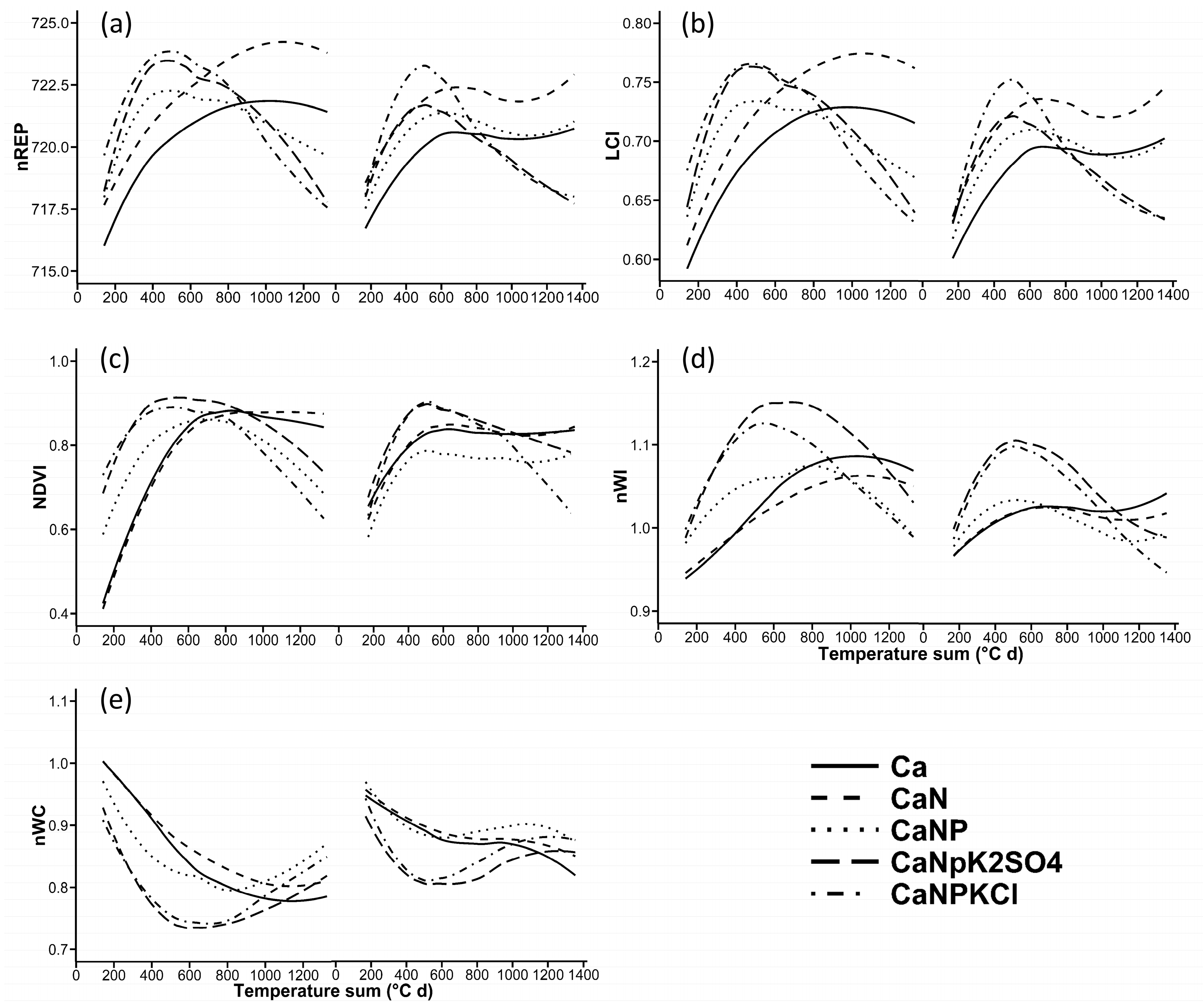
3.1. Seasonal Curves of the VIs

In Figure 2, the developments of narrowband Red Edge Position (nREP), Leaf Chlorophyll Index (LCI), NDVI, narrowband Water Index (nWI) and narrowband Water Content (nWC) by T∑ within the five plant communities are shown. These VIs were selected for visual presentation because they represent the best performing VIs for each group averaged over both growths of VIs according to Section 2.4, as well as the best performing VIs of each growth. Information on the performance of the eleven other VIs is attached in Supplement Table S8. The shape of the curves of all VIs measured in the Ca, CaN and CaNP treatment were more similar in Growth 2 than in Growth 1. This was mostly related to the lower amplitude of changes in VIs that we observed in Growth 2.

The curves of nREP, LCI, NDVI and nWI increased at the beginning of both growths in all plots. Thereby, the slopes of the curves derived for the NP(K)-treated plots were steeper than those in the Ca and CaN plot, but the CaNP treatment did not reach as high VI values as the NPK treatments. The T∑ at which peaks of these four VIs in the NP(K)-treated plots were reached differed between the VIs and between the two growths. The highest values in these four VIs were found at higher T∑s in Growth 1 than in Growth 2. Furthermore, the chlorophyll- and biomass-related VIs (nREP, LCI and NDVI) reached their peaks earlier than the water-related nWI. Towards the end of both growths, values of the four VIs decreased steeply in the NPK treatments. In contrast, VIs in the Ca and CaN plots remained relatively stable. Opposed to the four previously-mentioned VIs, the curve of nWC decreased at the beginning of both growths. Thereby, the highest decline rates were observed in the NP(K) treatments, which reached their minimum later in Growth 1 than in Growth 2. Afterwards, nWC in the NP(K) treatments began to rise. nWC in the Ca and CaN treatments decreased slower than in the NP(K) treatments at the beginning of both growths, but remained relatively stable towards their end.

In Growth 1, curves in the Ca, CaN and CaNP treatments featured differences in their values of nREP, LCI and nWC throughout most phases of the growing season. However, the curves measured in the CaNPKCl and CaNPK₂SO₄ treatments were similar in these three VIs. At the same time, these treatments differed considerably in nWI, particularly at the end of Growth 1. At the beginning of Growth 1, NDVI values were different between the plots. At later stages, NDVI values in the five plots became relatively similar. In Growth 2, larger differences between the CaNPKCl and the CaNPK₂SO₄ treatment were identified for nREP, LCI and NDVI than in Growth 1. In contrast, both NPK treatments showed similar courses of their curves for nWI and nWC.

3.2. Distinguishing the Grassland Communities Using the Welch Test

Although time courses of many VIs tested in this study followed similar patterns, uncertainty remained for how the identified differences have influenced the accuracy for classifying the grassland plots using one VI at a time.

Table 3. Ranks and overall accuracies of the 15 indices for the first and the second growth, as determined by the Welch test (12 < n < 33, p = 0.01, α = 0.99).

1st growth	Index	nWC	nWI	nLCI	nSIPI	LCI	nNDLI	NDVI	nNDNI
	Accuracy	0.91	0.85	0.84	0.84	0.83	0.83	0.80	0.80
	Index	nNDVI	nREP	GNDVI	nGNDVI	nNPCI	nPRI	nNPQI		Average
	Accuracy	0.79	0.79	0.76	0.75	0.73	0.68	0.41		0.77
2nd growth	Index	LCI	nWI	nREP	nSIPI	nWC	nLCI	nNDLI	nNDNI
	Accuracy	0.76	0.75	0.72	0.71	0.71	0.67	0.64	0.64
	Index	nGNDVI	nNDVI	NDVI	GNDVI	nNPCI	nNPQI	nPRI		Average
	Accuracy	0.62	0.62	0.61	0.61	0.46	0.46	0.44		0.63

displays the overall accuracies of the single VIs achieved using the Welch test. In the first growth, nWC significantly differed between the five plots in 91% of the cases and provided the highest rates of discrimination, followed by nWI, nLCI, narrowband Structure Intensive Pigment Index (nSIPI) and LCI. The weakest accuracy was achieved by narrowband Normalized Phaeophytization Index (nNPQI), followed by narrowband Photochemical Reflectance Index (nPRI), narrowband Normalized Pigment Chlorophyll Index (nNPCI) and narrowband Green Normalize Difference Vegetation Index (nGNDVI). In the second growth, significant differences in the VIs between the plots were most frequently found using LCI, nWI, nREP, nSIPI and nWC. As in Growth 1, the lowest classification rates in the second growth were reached with nPRI, nNPQI and NPCI.

Regarding the differences in classification accuracy reached by the broadband and narrowband versions of VIs, results between the two growths differed. In Growth 1, broadband NDVI and GNDVI outperformed their narrowband versions, whereas the opposite relation was found in Growth 2.

The probability for nREP, LCI, NDVI, nWC and nWI to distinguish plots at different T∑s correctly is shown in Figure 3. At the beginning of the first growth, accuracies of LCI, NDVI, nWI and nWC were above 80% and further increased to more than 95%. The accuracy of nREP was about 50% at the onset of growth, but drastically increased during the initial stages of Growth 1 and successfully separated more than 95% of the plots at a T∑ of 450 °C d. Afterwards, the accuracies of nREP, LCI and NDVI dropped to levels between 65% and 70%. Accuracies of nWC and nWI remained more stable, making them the strongest and second strongest VI, respectively. At the end of Growth 1, the accuracy of the chlorophyll-related VIs started to increase earlier than the accuracy of the water-related VIs. Thus, they achieved similar accuracies, like the water-related VIs.

During the onset of the second growth, the highest classification accuracies were reached using nWI (above 90%). Similar to the previous growth, the accuracies of all VIs (except for nREP) increased until T∑s of 400–450 °C d were reached. Afterwards, all VIs’ accuracies dropped, except for REP, which remained constant at this time. As LCI recovered as the first VI, it was the best performing VI between 800 and 1150 °C d. The water-related VIs recovered in their accuracies the latest. At the end of Growth 2, nREP steeply increased and outperformed the other four VIs.

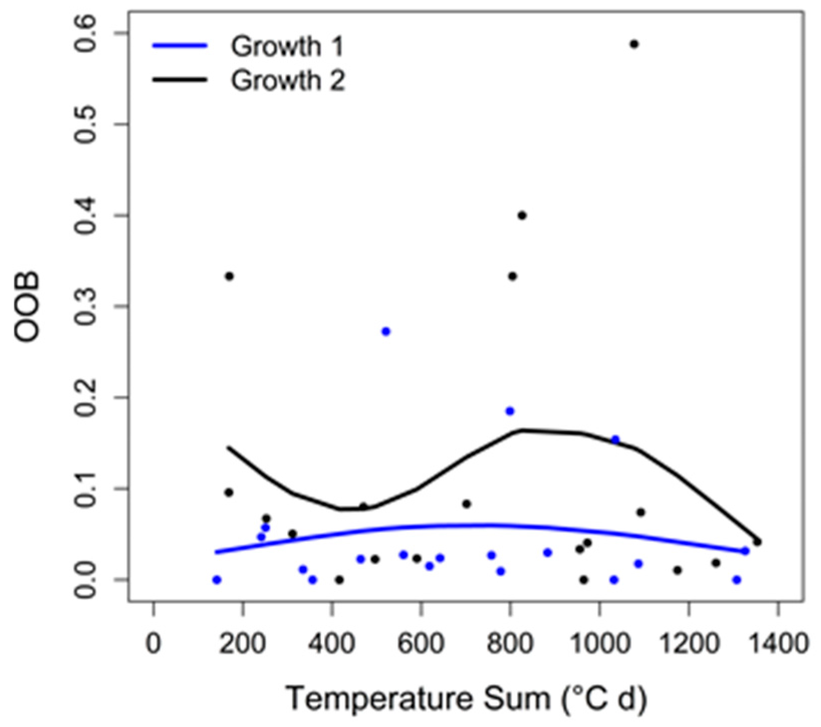
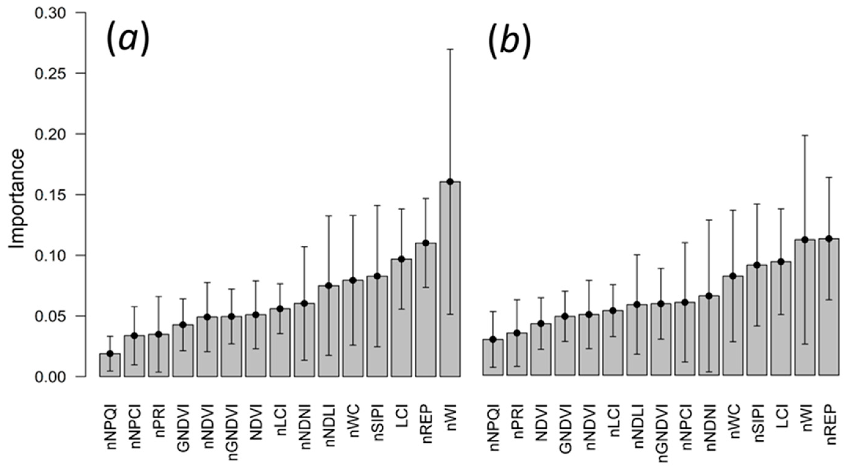
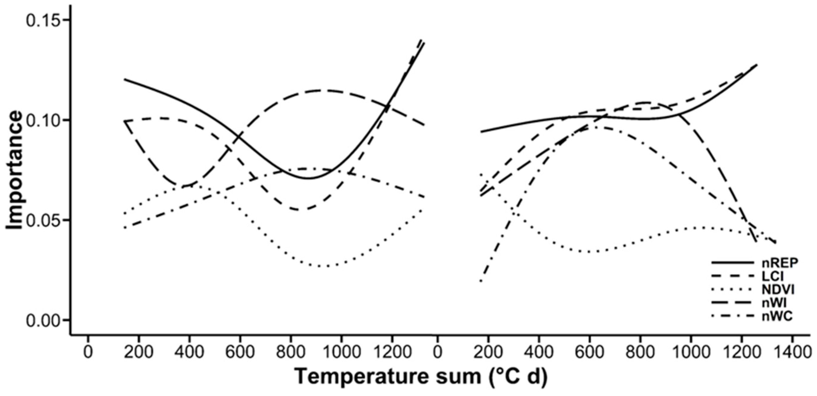
3.3. Random Forests Classification

The random forests classification was performed to investigate how the utilization of several VIs improves the classification accuracies, compared to single VIs. The error rate of the classification was expressed as OOB error, which is shown as a function of T∑ in Figure 4. It was observed that OOB errors in the second growth (12%) were higher than in the first growth (5%). Furthermore, the classification error in Growth 1 remained relatively stable (between 2.5% and 6%). In contrast, OOB errors in Growth 2 varied significantly with the T∑ and ranged between 2.5% and 17.5%.

To identify the probability of a VI for being selected as a split variable in random forests, the variable importance was calculated and averaged for each growth (Figure 5). The results of the t-test (cf.

Table A1. Performance of the fifteen VIs for distinguishing the five grassland communities in Growth 1 and Growth 2 (Welch test with α= 0.9; * p < 0.1; ** p < 0.05; *** p < 0.01, n = 19).

Growth 1

nWI

nREP

LCI

nSIPI

nWC

nNDLI

nNDNI

nLCI

NDVI

nGNDVI

nNDVI

GNDVI

nPRI

nNPCI

nNPQI

nWI

-

-

**

**

***

***

***

***

***

***

***

***

***

***

***

nREP

-

-

-

*

**

**

***

***

***

***

***

***

***

***

***

LCI

**

-

-

-

-

-

**

***

***

***

***

***

***

***

***

nSIPI

**

*

-

-

-

-

-

**

**

**

**

***

***

***

***

nWC

***

**

-

-

-

-

-

-

*

*

*

**

***

***

***

nNDLI

***

**

-

-

-

-

-

-

*

*

*

**

***

***

***

nNDNI

***

***

**

-

-

-

-

-

-

-

-

-

*

**

***

nLCI

***

***

***

**

-

-

-

-

-

-

-

-

**

**

***

NDVI

***

***

***

**

*

*

-

-

-

-

-

-

*

**

***

nGNDVI

***

***

***

**

*

*

-

-

-

-

-

-

*

*

***

nNDVI

***

***

***

**

*

*

-

-

-

-

-

-

-

**

***

GNDVI

***

***

***

***

**

**

-

-

-

-

-

-

-

**

***

nPRI

***

***

***

***

***

***

*

**

*

*

-

-

-

-

-

nNPCI

***

***

***

***

***

***

**

**

**

*

**

**

-

-

-

nNPQI

***

***

***

***

***

***

***

***

***

***

***

***

-

-

-

Growth 2

nREP

nWI

LCI

nSIPI

nWC

nNDNI

nNPCI

nGNDVI

nNDLI

nLCI

nNDVI

GNDVI

NDVI

nPRI

nNPQI

nREP

-

-

-

-

*

**

***

***

***

***

***

***

***

***

***

nWI

-

-

-

-

-

*

**

**

**

**

**

***

***

***

***

LCI

-

-

-

-

-

*

***

**

**

***

***

***

***

***

***

nSIPI

-

-

-

-

-

-

**

**

**

***

***

***

***

***

***

nWC

*

-

-

-

-

-

*

-

-

**

**

**

***

***

***

nNDNI

**

*

**

-

-

-

-

-

-

-

-

-

-

**

**

nNPCI

***

**

***

**

*

-

-

-

-

-

-

-

-

***

***

nGNDVI

***

**

**

**

-

-

-

-

-

-

-

-

-

*

**

nNDLI

***

**

**

**

-

-

-

-

-

-

-

-

-

*

*

nLCI

***

**

***

***

**

-

-

-

-

-

-

-

-

**

***

nNDVI

***

**

***

***

**

-

-

-

-

-

-

-

-

***

***

GNDVI

***

***

***

***

**

-

-

-

-

-

-

-

-

*

**

NDVI

***

***

***

***

***

-

-

-

-

-

-

-

-

*

*

nPRI

***

***

***

***

***

**

***

*

*

**

***

*

*

-

-

nNPQI

***

***

***

***

***

**

***

**

*

***

***

**

*

-

-

) indicate significant differences in the VIs’ importance. In the first growth, nWI reached the highest importance (16% of the decisions made) and was selected significantly more frequently than all other VIs, except for nREP, which ranked second. LCI, nSIPI, nWC and narrowband Normalized Difference Lignin Index (nNDLI) outperformed NDVI, nGNDVI, nNDVI, GNDVI, nPRI, nNPCI and nNPQI significantly. Medium to low importance (between 6% and 4%) was found for nNDNI, nLCI, NDVI, nGNDVI, nNDVI and GNDVI. These VIs have been of significantly higher importance than nNPCI and nNPQI. During the second growth, the differences in importance between the VIs were lower than in the first growth. However, similar VIs influenced the classification the strongest: nREP, nWI, LCI, nSIPI and nWC were of significantly higher importance than nLCI, nNDVI, GNDVI, NDVI, nPRI and nNPQI. Of medium to low importance were nNDNI, nNPCI, nGNDVI, nNDLI, nLCI, nNDVI, GNDVI and NDVI. nNPQI and nPRI were of significantly lower importance (2.9% and 3.5%, respectively) than all other VIs.

Figure 6 shows the variation in importance of nREP, LCI, NDVI, nWI and nWC throughout the growing season. At the beginning of Growth 1, nREP was most important for the classification. However, at T∑s above 400 °C d, the importance of all biomass and chlorophyll-related VIs (nREP, LCI and NDVI) decreased, whereas the importance of the water-related VIs (nWI and nWC) increased. Thus, at T∑s larger than 600 °C d, nWI was of highest importance, followed by nWC or nREP. After a T∑ of 900 °C d was reached, the importance of nWI and nWC decreased. Consequently, the classification was more influenced by chlorophyll-related VIs (particularly LCI and nREP) at T∑s larger than 1150 °C d. During the entire first growth, NDVI was among the VIs with the lowest importance.

At the onset of the second growth, nREP was the most important VI. However, over time, the importance of LCI and nWI increased and exceeded nREP at T∑s larger than 650 °C d. Similar to nWI, nWC increased in importance at the beginning of the second growth, but did not reach the high levels of nREP, LCI and nWI. At T∑s larger than 950 °C d, the importance of nWI decreased. Thus, during the remaining period of Growth 2, LCI or nREP featured the highest importance. Similar to Growth 1, NDVI had a minor impact on the classifications throughout the entire growth.

4. Discussion

4.1. Critical Reflection on the Experimental Settings

In this work, the performance of fifteen different VIs for distinguishing five differently-fertilized grassland communities (Ca, CaN, CaNP, CaNPKCl, CaNPK₂SO₄) was tested. Constant fertilization lead to a characteristic plant species composition in each plot, which differed between treatments and changed only marginally between years [23]. Similarly, biomass production varied between the plots; the lowest biomass was produced in the Ca treatment, followed by CaN, CaNP and the NPK treatments [21,22] (cf. Supplement Table S7).

Because observations were made in three years, it was assured that annual fluctuations in precipitation or radiation were captured in the dataset. This setup, as well as the utilization of T∑ as the temporal variable secured that no climatic or management factors influenced the species composition and the biomass development. Minor disturbances such as lodging of plants (especially at the end of the first growth in the NPK-treated plots) and the naturally-occurring variability of the plant canopies was diminished by acquiring measurements at three different locations within each plot. Stagakis et al. [45] identified significant effects of the sensor viewing angle and the sensor height on the spectral reflectance measured over plant communities. In this study, the utilization of the crane system allowed systematic measurements from a 2-m height and nadir position, which widely eliminated these effects. Changing cloud cover [26,46], as well as changes in solar elevation angle [45] are often considered as additional confounding factors of the spectral measurements. Diurnal changes in solar elevation were adapted by acquiring spectra between 10:00 a.m. and 4:00 p.m. and averaging this information for an entire day. Visual inspection of VI values recorded on the single days revealed that VI values were relatively stable. Furthermore, acquiring data in a large interval in time covered the daily occurring variance in spectral signal and further stabilized VI values. However, seasonal changes in solar elevation may have altered the irradiation conditions. However, we assume that these effects were minimized by utilizing VIs because their use significantly lowers the impact of illumination conditions and cloud cover (cf. [47]). Additionally, frequent measurements of the white reference panel ensured that reflectance was adapted for changes in solar irradiance.

4.2. Seasonal Curves of the VIs

Based on multitemporal measurements of five different VIs (nREP, LCI, NDVI, nWI and nWC) sensitive to different biophysical parameters, differences in the VI development over time were investigated. Comparing both growths, similar developments were observed. However, lower maxima of positively-developing VIs (nREP, LCI, NDVI and nWI), as well as higher minima for negatively-developing VIs (nWC) were observed in Growth 1. The reason behind this is that growth rates were lower in the second growth (cf. Supplement Table S7), resulting in lower intensities of green vegetation reflectance and lower amounts of water stored in plants.

As observed by other scientists [8,48], VIs followed strong seasonal dynamics throughout the growing season. In the NPK-fertilized plots, VIs related to biomass, as well as to chlorophyll and water content, such as nREP, LCI, NDVI and nWI, passed through a rapid increase at the beginning of both growths. At later stages, nREP, LCI and NDVI decreased as a result of starting senescence in the NPK-treated plots. This was supported by [13], who found significant effects of senesced grass components on the near-infrared reflectance, which has been used for the calculation of these VIs. In contrast, nWI remained at a high level for a longer time, indicating that water content stayed at a high level at the onset of senescence. At the time, NP(K) fertilized plots started senescing, all four VIs in the Ca and CaN plots increased because these plots host slow-growing species [23,24]. Such species not only increase in their biomass over a longer time-span, but also remain relatively constant in their water and chlorophyll content. nWC developed contrary to the four other VIs due to its negative response to water content.

4.3. Testing the Classification Accuracy of the Fifteen VIs Using the Welch Test

To test the ability of every single VI for distinguishing the five different vegetation communities, a Welch test was performed for each T∑. The average of the Welch tests’ results allowed an estimation of the overall classification accuracy of each VI in the individual growths. The average of the classification accuracies revealed that classification of all VIs (except nNPQI) was lower in Growth 2 than in Growth 1. The explanation for this is that VI curves in the second growth featured lower amplitudes and were less distinct from each other. These relatively low amplitudes were caused by a lower and more similar sward height and biomass production in Growth 2 (

Table A2. Averages and standard deviations of the Compressed Sward Height (CSH) measurements for 2013 and 2014.

Year	Growth	T∑ (°C d)	CSH (cm)	SD (CSH)
2013	1	947	20.59	10.63
	2	964	6.49	2.51
		1077	4.62	2.15
		1378	6.98	2.95
2014	1	464	5.52	2.93
		560	7.75	4.23
		757	18.12	8.47
		883	17.72	10.09
		1017	17.18	9.64
		1307	24.5	18.21
	2	210	5.17	1.18
		804	10.54	5.37
		972	12.94	4.90
		1174	13.28	4.97
		1353	11.21	4.57

).

At the beginning of both growths, classification accuracies were relatively low. We assume that this was caused by small differences in canopy biomass occurring at this stage. This is supported by measurements of Compressed Sward Height (CSH), which are highly correlated to canopy biomass [49]. CSH featured a standard deviation in compressed sward height between the five communities of 2.93 cm in the initial stage (464 °C d, 2014) and 18.21 cm in the final stage (464 °C d, 2014) of Growth 1 (Table A2). Similarly, a standard deviation of 1.18 cm was shown at the beginning (210 °C d, 2014) and 4.57 cm at the end (1353 °C d, 2014) of Growth 2 (Table A2). Furthermore, it is likely that subtle differences in the reflectance of the plant canopies in the early stages of both growths have been concealed by the influence of soil on the reflectance signal (cf. [18]). At later stages of the two growths, biomass increased steadily, which mitigating the contribution of soil reflectance to the spectral reflectance (cf. [2,50]). Combined with increasing differences in biomass occurring between the different fertilizer treatments, an increase in the classification accuracies was achieved. However, as soon as biomass production in the NPK-treated plots languished, classification accuracies dropped, as canopies were optically more similar.

Due to the onset of senescence in the NPK-treated plots, on the one hand, and the constant abundance of green biomass in the Ca and CaN plot, on the other hand, classification rates at the ends of both growths increased. This contradicts with results published by Fava et al. [10], who stated that the senescence of vegetation lowers the differences between VIs. We assume that the postponed onset of senescence in the Ca and CaN plots led to increased classification accuracies in this study. This is supported by Sanchez-Azofeifa et al. [51], who demonstrated that the ability to distinguish plant types based on spectral information is strongly dependent on their phenological stage.

During the first growth, the most successful separation in this experiment was achieved using nWC and nWI, which are known to respond to plant water content. The high overall classification rates of nWI and nWC were caused by the relatively stable classification accuracy in the middle of the growth. This stability was caused by differences in water holding capacity of the canopies because canopies featuring low biomass production (Ca and CaN treatments) desiccate earlier after rain events than the canopies of highly productive communities (NPK treatments). VIs coined for detecting changes in biomass, such as NDVI, as well as nNDVI, GNDVI and nGNDVI, achieved lower classification accuracies. The reason for the poor performance of these VIs is the strongly decreasing classification accuracy in the middle of the growths. An explanation for this decrease in classification accuracy are the saturation effects of these VIs, which were observed under high LAIs (cf. [52,53,54]). Interestingly, LCI, which is related to chlorophyll content, was less affected by saturation in the middle of the growth and seems to be more suitable for mapping grasslands featuring high LAIs than the previously-mentioned VIs. In the final stage of Growth 1, the classification accuracies of nREP and LCI increased and reached the accuracy level of nWI and NWC. This behavior is explained by the good performance of these VIs for distinguishing the senescing NPK treatments from the Ca and CaN treatments. nNPQI (related to phaeophytization), nPRI (indicating plant vitality) and nNPCI (related to chlorophyll content) achieved the lowest accuracies.

During the second growth, the highest classification accuracies were achieved by LCI, followed by nWI and nREP, which confirms the strong performances of these VIs found in Growth 1. The relatively good performance of LCI and nREP compared to the water content-related VIs in Growth 2 leads to the assumption that the lower LAIs support the utilization of chlorophyll- or biomass-related VIs. Again, our results indicate that nNPQI, nPRI and nNPCI, as well as the nGNDVI, nNDVI, NDVI and GNDVI are not well-suited for classifying our grassland communities. Finally, nWI and nSIPI, provided high classification accuracies for both growths, which suggests that these VIs are relatively stable for the classification of grasslands affected by different growing conditions.

No clear result was obtained whether broadband or narrowband VIs provide the highest accuracies for classifying the studies grassland communities. In Growth 1, broadband NDVI and GNDVI outperformed the narrowband versions, whereas in Growth 2, the narrowband versions provided higher classification accuracies. These results contradict the findings made by Thenkabail et al. [55], who found an increased classification accuracy using exclusively narrowbands to separate weeds, shrubs, crops and grasses in Africa compared to a classification using exclusively broadbands. This suggests that the selection of broadband or narrowband VIs for achieving optimal classification is also dependent upon the timing of spectral data acquisition.

4.4. Random Forests Classification

We applied a random forests classification to investigate how much the inclusion of all fifteen VIs improved the classification of the five plots compared to single VIs. Our results show that classification accuracy increased by 4% in Growth 1 and 12% in Growth 2 in comparison to the strongest VI using the Welch test. Furthermore, the classification accuracy achieved by random forests was more stable (remaining always above 82%) than the best performing VIs identified using the Welch test. In Growth 1, classification rates varied marginally over time, whereas OOB errors in Growth 2 fluctuated between 2.5% and 17.5%. These variations in Growth 2 and the resulting lower overall accuracy were most likely caused by larger influences of soil reflectance on the signal (cf. [2]) at the beginning of Growth 2, as well as by smaller differences in between the plots’ canopy biomasses in the green-up phase (Table A2). The increasing classification accuracy at the end of Growth 2 was caused by the onset of senescence in the NPK-treated plots, whereas the other plots remained stable in their amount of green leaf area (cf. [56]).

Variable importance indicates the frequency a VI is selected inside a random forest. In Growth 1, nWI was the most important VI, followed by nREP and LCI. Our results show that other VIs, such as nSIPI, nNDLI, nNDNI and nLCI, carry additional important information for improving the classification. Interestingly, other biomass-related VIs (i.e., NDVI, nGNDVI, nNDVI and GNDVI), as well as water-related VIs (i.e., nWC) were of relatively low importance compared to the Welch test. We assume that nWI as a water-related VI, as well as nREP and LCI as chlorophyll-related VIs carried redundant information and lead to the low importance of these VIs. Of minor importance were nPRI, nNPCI and nNPQI, which indicates that these VIs marginally support the classification. In the second growth, the ranking in importance of the VIs was similar, but the weight of the VIs was more evenly distributed. This even distribution supports the assumption that especially if classification accuracy was low using single VIs, the addition of VIs sensitive to other biophysical variables increased the classification accuracy. Therefore, nREP as the most important VI was closely followed by nWI, LCI, nSIPI and nNDNI. As biomass-related VIs were less influenced by the high LAIs in Growth 2, nGNDVI and nNPCI increased in importance compared to Growth 1. As these two VIs included similar information as nNDVI, GNDVI and NDVI, the latter VIs were of lower importance. As observed in the first growth, nPRI and nNPQI were rarely selected by random forests.

Using nREP, LCI, NDVI, nWI and nWC, the importance of the VIs under changing T∑s was investigated. In Growth 1, the results of variable importance widely confirmed our findings made using the Welch test. It was shown that the importance of water-related VIs was relatively stable at times when biomass- and chlorophyll-related VIs saturated due to high LAIs of the grass canopies (cf. [52,53,54]). NDVI was of low importance throughout the entire first growth, which confirms its low classification accuracy identified using the Welch test. Throughout the entire second growth, the chlorophyll-related VIs nREP and LCI were relatively stable in their importance. However, nWI and nWC added valuable information especially at T∑s between 400 and 1000 °C d, indicating that these VIs are particularly important when LAIs in the canopies are high and obscure differences in biomass or chlorophyll content. Again, NDVI was of minor importance.

5. Conclusions

This study presents an approach for classifying grassland communities along a gradient from intensive to extensive fertilizer management in a two-cut-system using a set of fifteen remotely-sensed vegetation indices (VIs). It was shown that VIs are useful to identify differences between the grassland communities at different times throughout a growing season. Each VI featured characteristic fluctuations over time in the individual plots. It is well documented for this particular experiment that plots differ significantly in their biophysical properties, such as biomass production. Hence, we conclude that the VIs that we tested were sensitive to these properties.

The different time courses of VI development have far-reaching consequences for the use and interpretation of VIs when classifying grassland. None of the VIs was able to feature constantly high classification accuracies throughout the entire growing season. However, while classification accuracies of VIs sensitive to one biophysical variable decreased, the accuracies of other VIs remained more stable allowing higher classification accuracies. Biomass- or chlorophyll-related VIs, such as nREP, NDVI or LCI, provided good results when plants had further developed in the intensively-managed plots than in the extensively-managed plots. However, at later stages when the extensively-managed plots caught up in development, water content-related VIs, such as nWI or nWC, were the better alternative for a classification because biomass-related VIs were affected by saturation effects. Further, classification in the second growth was more difficult than in the first growth, due to less distinct differences in biophysical characteristics in between the plant communities. Thereby, the classification performed particularly weak when slow-growing canopies had fully developed and fast-growing canopies had not yet entered senescence. At this stage, nWI and nWC did not reach the high classification accuracies they reached in the Growth 1, so that none of the VIs separated the communities reliably.

This problem was solved by applying all fifteen VIs in the random forests algorithm. A time series of random forest models using the best VIs for classifying the plant communities was created.

As spectral information in this procedure was used more effectively, classification accuracies increased in both growths, but most considerably in the second growth. Furthermore, our multitemporal analysis has shown that classification accuracies using this approach remained relatively stable throughout the entire first growth. Although classification rates in the second varied to some degree, significant improvements were made compared to the utilization of single VIs.

These results suggest that the selection of an appropriate VI (depending on the plant development) is essential for classifying grasslands using single VIs. However, an alternative using random forests was promising, because it yielded a more robust grassland classification.

The utilization of this multi-VI approach for grassland mapping at larger spatial extent could improve the separation of designated plant communities with respect to their floristic composition and plant properties. Future research should be guided towards testing random forests classifiers using VIs for grassland mapping with aerial or satellite imagery for other grassland communities featuring higher or lower temporal variability in biomass production and spectral reflectance. Results of such studies may significantly improve existing monitoring techniques (e.g., using single VIs), improve grassland mapping and contribute to a more sustainable management of grassland ecosystems.

References

1. Price, K.P.; Crooks, T.J.; Martinko, E.A. Grasslands across time and scale: A remote sensing perspective. Photogramm. Eng. Remote Sens. 2001, 67, 414–420. [Google Scholar]
2. Schut, A.G.T.; Ketelaars, J.J.M.H.; Meulemann, J.; Kornet, J.G.; Lockhorst, C. Novel imaging spectroscopy for grass sward characterization. Biosyst. Eng. 2002, 82, 131–141. [Google Scholar] [CrossRef]
3. Gianelle, D.; Vescovo, L. Determination of green herbage ratio in grasslands using spectral reflectance. Methods and ground measurements. Int. J. Remote Sens. 2007, 28, 931–942. [Google Scholar] [CrossRef]
4. Cornelissen, J.H.C.; Lavorel, S.; Garnier, E.; Diaz, S.; Buchmann, N.; Gurvich, D.E.; Reich, P.B.; ter Steege, H.; Morgan, H.D.; van der Heijden, M.G.A.; et al. A handbook of protocols for standardised and easy measurement of plant functional traits worldwide. Aust. J. Bot. 2003, 51, 335–380. [Google Scholar] [CrossRef]
5. Aragón, R.; Oesterheld, M. Linking vegetation heterogeneity and functional attributes of temperate grasslands through remote sensing. Appl. Veg. Sci. 2008, 11, 117–130. [Google Scholar] [CrossRef]
6. Hill, M.J. Vegetation index suites as indicators of vegetation state in grassland and savanna: An analysis with simulated SENTINEL 2 data for a North American transect. Remote Sens. Environ. 2013, 137, 94–111. [Google Scholar] [CrossRef]
7. Wardlow, B.D.; Egbert, S.L.; Kastens, J.H. Analysis of time-series MODIS 250 m vegetation index data for crop classification in the U.S. Central Great Plains. Remote Sens. Environ. 2007, 108, 290–310. [Google Scholar] [CrossRef]
8. Psomas, A.; Zimmermann, N.E.; Kneubühler, M.; Kellenberger, T.; Itten, K. Seasonal variability in spectral reflectance for discriminating grasslands along a dry-mesic gradient in Switzerland. In Proceedings of the 4th EARSeL Workshop on Imaging Spectroscopy, New Quality in Environmental Studies, Warsaw, Poland, 27–30 April 2005.
9. Poças, I.; Cunha, M.; Pereira, L.S. Dynamics of mountain semi-natural grassland meadows inferred from SPOT-VEGETATION and field spectroradiometer data. Int. J. Remote Sens. 2012, 33, 4334–4355. [Google Scholar] [CrossRef]
10. Fava, F.; Colombo, R.; Bocchi, S.; Meroni, M.; Sitzia, M.; Fois, N.; Zucca, C. Identification of hyperspectral vegetation indices for Mediterranean pasture characterization. Int. J. Appl. Earth Obs. Geoinf. 2009, 11, 233–243. [Google Scholar] [CrossRef]
11. Daughtry, C.S.T.; Walthall, C.L.; Kim, M.S.; Brown de Colstoun, E.; McMurtey, J.E. Estimating corn leaf chlorophyll concentration from leaf and canopy reflectance. Remote Sens. Environ. 2000, 74, 229–239. [Google Scholar] [CrossRef]
12. He, Y.; Guo, X.; Wilmshurst, J. Studying mixed grassland ecosystems I: Suitable hyperspectral vegetation indices. Can. J. Remote Sens. 2006, 32, 98–107. [Google Scholar] [CrossRef]
13. Asner, G.P. Biophysical and Biochemical Sources of Variability in Canopy Reflectance. Remote Sens. Environ. 1998, 64, 234–253. [Google Scholar] [CrossRef]
14. Kumar, L.; Schmidt, K.; Dury, S.; Skidmore, A. Imaging spectrometry and vegetation science. In Imaging Spectrometry; van de Meer, F., de Jong, S.M., Eds.; Springer: Dordrecht, The Netherlands, 2002; pp. 111–155. [Google Scholar]
15. Lucas, R.M.; Honzak, M.; Foody, G.M.; Curran, P.J.; Corves, C. Characterizing tropical secondary forests using multi-temporal Landsat sensor imagery. Int. J. Remote Sens. 1993, 14, 3061–3067. [Google Scholar] [CrossRef]
16. Roberts, D.A.; Numata, I.; Holmes, K.; Batista, G.; Krug, T.; Monteiro, A.; Powell, B.; Chadwick, O.A. Large area mapping of land-cover change in Rondonia using multitemporal spectral mixture analysis and decision tree classifiers. J. Geophys. Res. Atmos. 2002, 107, D20. [Google Scholar] [CrossRef]
17. Adams, J.B.; Sabol, D.E.; Kapos, V.; Almeida Filho, R.; Roberts, D.A.; Smith, M.O.; Gillespie, A.R. Classification of multispectral images based on fractions of endmembers: Application to land-cover change in the Brazilian Amazon. Remote Sens. Environ. 1995, 52, 137–154. [Google Scholar] [CrossRef]
18. Numata, I.; Roberts, D.A.; Chadwick, O.A.; Schimel, J.P.; Galvao, L.S.; Soares, J.V. Evaluation of hyperspectral data for pasture estimate in the Brazilian Amazon using field and imaging spectrometers. Remote Sens. Environ. 2008, 112, 1569–1583. [Google Scholar] [CrossRef]
19. Welch, B.L. The significance of the difference between two means when the population variances are unequal. Biometrika 1938, 29, 350–362. [Google Scholar] [CrossRef]
20. Breiman, L. Random forests. Mach. Learn. 2001, 45, 5–32. [Google Scholar] [CrossRef]
21. Schellberg, J.; Möseler, B.M.; Kühbauch, W.; Rademacher, I.F. Long-term effects of fertilizer on soil nutrient concentration, yield, forage quality and floristic composition of a hay meadow in the Eifel mountains, Germany. Grass Forage Sci. 1999, 54, 195–207. [Google Scholar] [CrossRef]
22. Hejcman, M.; Češková, M.; Schellberg, J.; Pätzold, S. The Rengen Grassland Experiment: Effect of Soil Chemical Properties on Biomass Production, Plant Species Composition and Species Richness. Folia Geobot. 2010, 45, 125–142. [Google Scholar] [CrossRef]
23. Hejcman, M.; Klaudisová, M.; Schellberg, J.; Honsová, D. The Rengen Grassland Experiment: Plant species composition after 64 years of fertilizer application. Agric. Ecosyst. Environ. 2007, 122, 259–266. [Google Scholar] [CrossRef]
24. Chytrý, M.; Hejcman, M.; Hennekens, S.M.; Schellberg, J. Changes in vegetation types and Ellenberg indicator values after 65 years of fertilizer application in the Rengen Grassland Experiment, Germany. Appl. Veg. Sci. 2009, 12, 167–176. [Google Scholar] [CrossRef]
25. Thenkabail, P.S.; Smith, R.B.; De Pauw, E. Evaluation of narrowband and broadband vegetation indices for determining optimal hyperspectral wavebands for agricultural crop characterization. Photogramm. Eng. Remote Sens. 2002, 68, 607–622. [Google Scholar]
26. Gamon, J.A.; Cheng, Y.; Claudio, H.; MacKinney, L.; Sims, D.A. A mobile tram system for systematic sampling of ecosystem optical properties. Remote Sens. Environ. 2006, 103, 246–254. [Google Scholar] [CrossRef]
27. Ritchie, J.T.; NeSmith, D.S. Temperature and crop development. In Modeling Plant and Soil Systems; Hanks, J., Ritchie, J.T., Eds.; Agron. Monogr. ASA; CSSA; SSSA: Madison, WI, USA, 1991; pp. 5–29. [Google Scholar]
28. DWD [Deutscher Wetterdienst] 1 × 1 km Wetterdaten. Available online: http://www.dwd.de/DE/leistungen/webwerdis/webwerdis.html (accessed on 15 May 2016).
29. Ernst, P.; Loeper, E.G. Temperaturentwicklung und Vegetationsbeginn auf dem Grünland. Wirtschaftseigene Futter 1976, 22, 5–11. [Google Scholar]
30. BlackBridge (Ed.) Spectral Response curves of the RapidEye Sensor. Available online: http://blackbridge.com/rapideye/upload/Spectral_Response_Curves.pdf (accessed on 20 January 2016).
31. Cleveland, W.S.; Grosse, E.; Shyu, W.M. Local regression models. In Statistical Models in S; Chambers, J.M., Hastie, T.J., Eds.; Chapman & Hall: Boca Raton, FL, USA, 1992; pp. 309–377. [Google Scholar]
32. Wickham, H.; Chang, W. (Eds.) ggplot2. Available online: https://cran.r-project.org/web/packages/ggplot2/index.html (accessed on 13 January 2017).
33. R Development Core Team. R: A Language and Environment for Statistical Computing; R Foundation for Statistical Computing: Vienna, Austria, 2015. [Google Scholar]
34. Gitelson, A.A.; Kaufman, Y.J.; Merzlyak, M.N. Use of a green channel in remote sensing of global vegetation from EOS-MODIS. Remote Sens. Environ. 1996, 58, 289–298. [Google Scholar] [CrossRef]
35. Rouse, J., Jr.; Haas, R.; Schell, J.; Deering, D. Monitoring vegetation systems in the Great Plains with ERTS. NASA Spec. Publ. 1974, 351, 309–317. [Google Scholar]
36. Guyot, G.; Baret, F.; Major, D.J. High spectral resolution: Determination of spectral shifts between the red and the near infrared. Int. Arch. Photogramm. Remote Sens. 1988, 11, 750–760. [Google Scholar]
37. Datt, B. A new reflectance index for remote sensing of chlorophyll content in higher plants: Tests using eucalyptus leaves. J. Plant Physiol. 1999, 154, 30–36. [Google Scholar] [CrossRef]
38. Peñuelas, J.; Gamon, J.A.; Fredeen, A.L.; Merino, J.; Field, C.B. Reflectance indices associated with physiological changes in nitrogen- and water-limited sunflower leaves. Remote Sens. Environ. 1994, 48, 135–146. [Google Scholar] [CrossRef]
39. Serrano, L.; Peñuelas, J.; Ustin, S.L. Remote sensing of nitrogen and lignin in Mediterranean vegetation from AVIRIS data: Decomposing biochemical from structural signals. Remote Sens. Environ. 2002, 81, 355–364. [Google Scholar] [CrossRef]
40. Underwood, E.; Ustin, S.; Dipietro, D. Mapping nonnative plants using hyperspectral imagery. Remote Sens. Environ. 2003, 86, 150–161. [Google Scholar] [CrossRef]
41. Peñuelas, J.; Pinol, J.; Ogaya, R.; Filella, I. Estimation of plant water concentration by the reflectance Water Index WI (R900/R970). Int. J. Remote Sens. 1997, 18, 2869–2875. [Google Scholar] [CrossRef]
42. Peñuelas, P.; Filella, I.; Lloret, P.; Munoz, F.; Vilajeliu, M. Reflectance assessment of mite effects on apple trees. Int. J. Remote Sens. 1995, 16, 2727–2733. [Google Scholar] [CrossRef]
43. Barnes, J.D.; Balaguer, L.; Manrique, E.; Elvira, S.; Davison, A.W. A reappraisal of the use of DMSO for the extraction and determination of chlorophylls a and b lichens and higher plants. Environ. Exp. Bot. 1992, 32, 85–100. [Google Scholar] [CrossRef]
44. Chambers, J.M.; Hastie, T.J. (Eds.) Statistical Models in S; Chapman & Hall: Boca Raton, FL, USA, 1992.
45. Stagakis, S.; Markos, N.; Sykioti, O.; Kyparissis, A. Monitoring canopy biophysical and biochemical parameters in ecosystem scale using satellite hyperspectral imagery: An application on a Phlomis fruticosa Mediterranean ecosystem using multiangular CHRIS/PROBA observations. Remote Sens. Environ. 2010, 114, 977–994. [Google Scholar] [CrossRef]
46. Roelofsen, H.; van Bodegom, P.; Kooistra, L.; Witte, J.P. Trait Estimation in Herbaceous Plant Assemblages from in situ Canopy Spectra. Remote Sens. 2013, 5, 6323–6345. [Google Scholar] [CrossRef]
47. Jensen, J.R. (Ed.) Remote Sensing of the Environment. An Earth Resource Perspective, 2nd ed.; Pearson Prentice Hall: Upper Saddle River, NJ, USA, 2007.
48. Rossini, M.; Cogliati, S.; Meroni, M.; Migliavacca, M.; Galvagno, M.; Busetto, L.; Cremonese, E.; Juliatta, T.; Siniscalco, C.; Morra di Cella, U.; et al. Remote sensing-based estimation of gross primary production in a subalpine grassland. Biogeosciences 2012, 9, 2565–2584. [Google Scholar] [CrossRef] [Green Version]
49. Harmoney, K.R.; Moore, K.J.; George, J.R.; Brummer, E.C.; Russell, J.R. Determination of pasture biomass using four indirect methods. Agron. J. 1997, 89, 665–672. [Google Scholar] [CrossRef]
50. Norman, J.M.; Welles, J.M.; Walter, E.A. Contrasts among bidirectional reflectance of leaves, canopies, and soils. IEEE Trans. Geosci. Remote Sens. 1985, 23, 659–667. [Google Scholar] [CrossRef]
51. Sánchez-Azofeifa, G.A.; Castro, K.; Wright, S.J.; Gamon, J.; Kalacska, M.; Rivard, B.; Schnitzler, S.A.; Feng, J.L. Differences in leaf traits, leaf internal structure, and spectral reflectance between two communities of lianas and trees: Implications for remote sensing in tropical environments. Remote Sens. Environ. 2009, 113, 2076–2088. [Google Scholar] [CrossRef]
52. Lorenzen, B.; Jensen, A. Reflectance of blue, green, red and near infrared radiation from wetland vegetation used in a model discriminating live and dead above ground biomass. New Phytol. 1998, 108, 345–355. [Google Scholar] [CrossRef]
53. Wang, Q.; Adiku, A.; Tenhunen, J.; Granier, A. On the relationship of NDVI with leaf area index in a deciduous forest site. Remote Sens. Environ. 2005, 94, 244–255. [Google Scholar] [CrossRef]
54. Cho, M.A.; Skidmore, A.; Corsi, F.; Van Wieren, S.E.; Sobhan, I. Estimation of green grass/herb biomass from airborne hyperspectral imagery using spectral indices and partial least squares regression. Int. J. Appl. Earth Obs. Geoinf. 2007, 9, 414–424. [Google Scholar] [CrossRef]
55. Thenkabail, P.S.; Enclona, E.A.; Ashton, M.S.; Van der Meer, B. Accuracy assessments of hyperspectral waveband performance for vegetation analysis applications. Remote Sens. Environ. 2004, 91, 354–376. [Google Scholar] [CrossRef]
56. Idso, S.B.; Pinter, P.J., Jr.; Jackson, R.D.; Reginato, R.J. Estimation of grain yields by remote sensing of crop senescence rates. Remote Sens. Environ. 1980, 9, 87–91. [Google Scholar] [CrossRef]
Figure 1. Setup of the automated field observation system with its components (a) and arrangement of fertilizer treatments and monitoring plots (b).
Remotesensing 09 00081 g001
Figure 2. Smoothed curves of temporal development of (a) nREP, (b) LCI, (c) NDVI, (d) nWI and (e) nWC in Growing Seasons 1 and 2.
Remotesensing 09 00081 g002
Figure 3. Accuracies of nREP, LCI, NDVI, nWI and nWC to distinguish plots at different T∑s. Raw data, including single data points, are deposited in Supplement Tables S5 and S6.
Remotesensing 09 00081 g003
Figure 4. Random forests: Out-Of-Bag (OOB) errors of Growths 1 and 2.
Remotesensing 09 00081 g004
Figure 5. Overall importance of the VIs in the random forests classification for Growth 1 (a) and Growth 2 (b). The error bars indicate the standard deviation in overall importance calculated from the importance derived for the single T∑s.
Remotesensing 09 00081 g005
Figure 6. Importance of nREP, LCI, NDVI, nWI and nWC in Growth 1 and Growth 2. For single data points, see Supplement Tables S5 and S6.
Remotesensing 09 00081 g006