Article

Mapping Extent Dynamics of Small Lakes Using Downscaling MODIS Surface Reflectance

1
State Key Laboratory of Resources and Environmental Information System, Institute of Geographic Sciences and Natural Resources Research, Chinese Academy of Sciences, Beijing 100101, China
2
University of Chinese Academy of Sciences, Beijing 100049, China
3
Global Land Cover Facility, Department of Geographical Sciences, University of Maryland, College Park, MD 20742, USA
4
Department of Ecological Remote Sensing, Satellite Environment Center, Ministry of Environmental Protection, Beijing 100094, China
5
US Department of Agriculture Forest Service, Region 5, Remote Sensing Laboratory, McClellan, CA 95652, USA
6
College of Tourism and Environment, ShaanXi Normal University, Xi’an 710100, China
*
Author to whom correspondence should be addressed.
Submission received: 11 November 2016 / Revised: 28 December 2016 / Accepted: 11 January 2017 / Published: 17 January 2017

Abstract

:
Lake extent is an indicator of water capacity as well as the aquatic ecological and environmental conditions. Due to the small sizes and rapid water dynamics, monitoring the extent of small lakes fluctuating between 2.5 and 30 km2 require observations with both high spatial and temporal resolutions. The paper applied an improved surface reflectance (SR) downscaling method (i.e., IMAR (Improved Modified Adaptive Regression model)) to downscale the daily SR acquired by the Moderate Resolution Imaging Spectroradiometer (MODIS) Terra platform to a consistent 250-m resolution, and derived monthly water extent of four small lakes in the Tibetan Plateau (Longre Co, Ayonggongma Co, Ayonggama Co, and Ayongwama Co)) from 2000 to 2014. Using Landsat ETM+ acquired on the same date, the downscaled MODIS SR and identified water extent were compared to the original MODIS, observations downscaled using an early SR downscaling method (MAR (Modified Adaptive Regression model)) and Wavelet fusion. The results showed IMAR achieved the highest correlation coefficients (R2) (0.89–0.957 for SR and 0.79–0.933 for water extent). The errors in the derived water extents were significantly decreased comparing to the results of MAR and Wavelet fusion, and lakes morphometry of IMAR is more comparable to Landsat results. The detected lake extents dynamic between 2000 and 2014 were analyzed using the trend and season decomposition model (BFAST), indicating an increasing trend after 2005, and it likely had higher correlations with temperature and precipitation variation in the Tibetan region (R2: 0.598–0.728 and 0.61–0.735, respectively).

Graphical Abstract

1. Introduction

Lakes only cover a small portion of the global land, but they are essential components of the hydrosphere and water cycle, and their distributions over space and time greatly alter the Earth’s surface conditions and influence the general circulation of the atmosphere. In addition, water dynamic of lakes may lead to disasters such as flooding, outbreaks of waterborne disease and water shortage in dry tropical areas, which may involve loss of lives [1]. Thus, monitoring the dynamic of lakes is essential for terrestrial ecosystems and human civilization. However, previous study mainly focuses on large lake extent (two-dimension coverage of lakes), because it has very strong correlation with the water capacity, and it is a robust indicator of lake water dynamic. Small lakes have been widely ignored in virtually all global processes and cycles, while small lakes and ponds dominate the areal extent of continental water [2]; recently, small-scale lakes in the Tibetan Plateau and its surrounding areas are getting worse owing to ecological deterioration caused by human disturbance [3]. Serious environmental problems have been reported for numerous lakes in the area, such as eutrophication, salinization and pollution caused by the increased human pressure [4]. The remoteness, high altitude, thin atmosphere and harsh weather conditions in western China make it difficult to monitor the conditions of lakes using field observations.
However, remote sensing has become a foremost technique for monitoring land surface processes (i.e., lakes dynamics and forest change), because Earth surface observations can be obtained periodically by satellite sensors [5]. Studies related to lakes dynamics have been done using data acquired from many remote sensing sensors, such as Landsat-5 TM (Thematic Mapper), Landsat-7 ETM+ (Enhanced Thematic Mapper Plus), Quickbird, WorldView, IKONOS and MODIS, SPOT, ASTER (Advanced Space borne Thermal Emission and Reflection Radiometer), ALOS AVNIR-2 (Advanced Visible and Near Infrared Radiometer type 2) and PALSAR (Phased Array type L-band Synthetic Aperture Radar), etc. [6], which make it possible to accurately detect and delineate water body information [7,8,9]. Inland small water bodies intend to have fast variation due to flooding, drought, irrigation and hydropower station construction. Satellite sensors, such as TM, ETM+, and SPOT, have relatively higher spatial resolution, but longer revisiting cycles make it difficult for monitoring the rapid dynamics of lakes. MODIS provides daily observations, and it is particularly suitable for detecting water body dynamic [10]; however, the majority of its spectral bands, especially the water sensitive SWIR bands, are observed at 500-m resolution, which limits the capability for monitoring small lakes [11]. For example, the normalized difference water index (NDWI) was commonly used to extract water body boundary, which is designed based on both green and near infrared (NIR) bands [12]. Xu [13] proposed the modified NDWI (MNDWI), which replaced NIR band with SWIR band. Ji et al. [14] suggested that the MNDWI has a more stable threshold than other WIs. Feyisa et al. [1] proposed two versions of an automated water extraction index (AWEI), namely AWEInsh (i.e., with no shadow) and AWEIsh (i.e., with shadow), which require six MODIS bands.
Downscaling methods establish models between observations at their native coarser resolution and a finer resolution reference to estimate the observations at the finer resolution. Applying the methods to MODIS daily observation will produce daily multi-spectral estimates at a finer resolution, which is in favor of monitoring small lakes dynamics [6]. MODIS images, as a common source of remote sensing imagery used for global monitoring, contain 36 spectral bands, including two 250-m spatial resolution bands (Bands 1–2), five 500-m bands (Bands 3–7) and 29 1-km bands. Numerous methods have been developed to take the advantage of the finer resolution bands to downscale the coarser resolution bands. For example, Discrete Wavelet Transform (DWT) fusion method was used to generate related finer resolution images, which, in general, had lower visual interpretation [15]. An adaptive regression model was proposed for every generic scene type (vegetation, desert/barren land, snow, water and cloud), combining MODIS bands 3–7 with band 1, band 2 and Normalized Difference Vegetation Index (NDVI) to obtain bands 3–7 SR at 250-m resolution. The adaptive regression model was built on MODIS MOD 02-Level-1B calibrated and geo-located at-aperture radiances product (MOD02HKM/MOD02QKM) without atmospheric conditions correction. To build an adaptive regression model, therefore, atmospheric correction was required to adjust for atmospheric scattering and absorption effects, and a generic land cover classification was needed, which indicated complicated and time-consuming processing steps [6]. Recently, geostatistical solutions, as a family of image fusion methods, have received increasing attention in image downscaling, such as Kriging with external drift (KED) [16] and area-to-point regression Kriging (ATPRK) [17]. Although geostatistical solutions solve the issue of preserving the spectral properties of the observed coarse images, these methods suffer from expensive computational cost because of semi-variogram modeling procedure. To eliminate the weakness of adaptive regression model, a downscaling method based on the modified adaptive regression model (MAR) was presented towards extracting water bodies from MODIS SR at 250-m resolution, but MAR has two limitations [6]. First, few uneven surface reflection (SR) values can be observed, especially at the transition boundary of different land cover types because of excessive enhancement caused by equally weighted average method for retaining the spectral properties. Second, non-linear regression in MAR had resulted in some outliers on the water bodies. The objective of this paper is to introduce an improved MODIS SR downscaling method to address the issues in MAR; identify and analyze water extents of four lakes in Tibetan Plateau in the past 15 years (2000–2014) using the daily downscaled 250-m resolution MODIS observations.

2. Study Area and Data Source
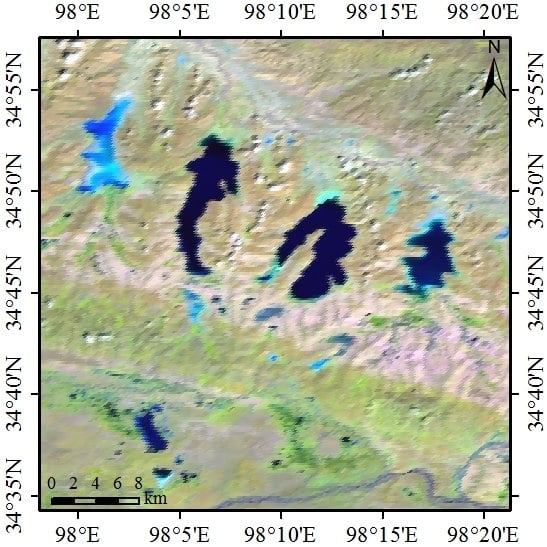
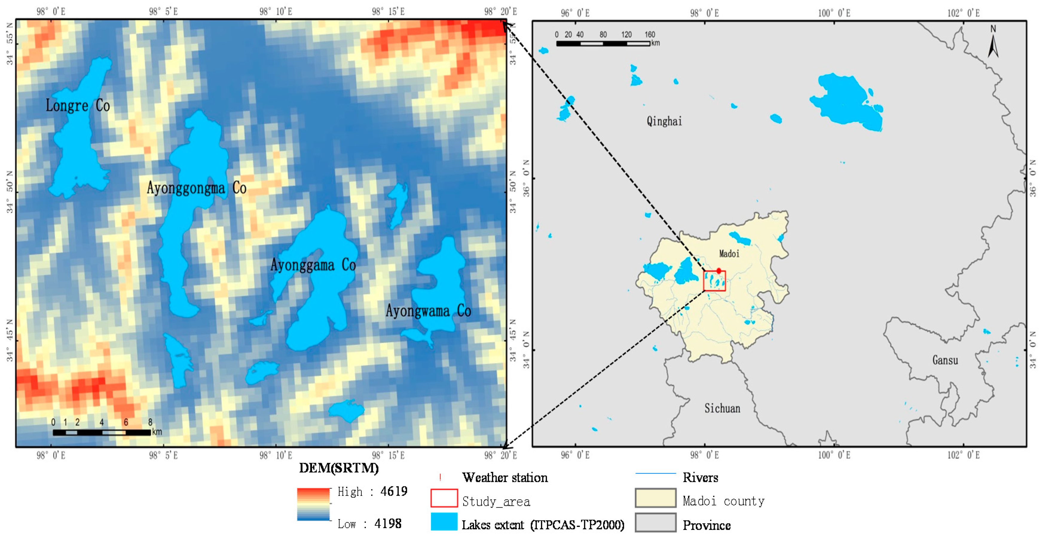
2.1. Study Area

Of 1055 lakes in Tibetan plateau (TP) [18], this paper focuses on four lakes located in the center of Madoi County of Qinghai province because of the large historical extent variation and their complex shapes, allowing investigating the performance of method (Figure 1) [19]. The area of Madoi County is about 25,000 km2, and with an average elevation of 4,300 m, it is the highest Chinese county by average elevation. The main type of land use in Madoi County is grassland, nearly 77.93% of the total area, and grassland was degraded to sand [20]. According to Chinese Lakes, the areas of four lakes are 19, 29.3, 37.6 and 22.7 km2, respectively, and they are supplied by rivers in the south and precipitation. Average annual temperature in the lakes catchment is −4.1 °C, and the annual precipitation is around 303.9 mm, which is measured by the weather station in the north as Figure 1 shows [21]. Flooding and drought events have been recorded in Madoi County. For example, only four short periods of precipitation were recorded between May to October 2001, which caused a severe drought in the county [22]; a long and continuous precipitation was recorded between 15 and 19 June 2007, which led to the dramatic extent increase of the lakes [23]. For the largest lakes (Lake Zhaling and Eling) in Madoi County, a pumped-storage power station was built in northern Lake Eling in 1998 [23], making it difficult to analyze environment response for the lake dynamics. Conversely, Longre Co (lake I, 34°52′N, 98°55′E), Ayonggongma Co (lake II, 34°49′N, 98°06′E), Ayonggama Co (lake III, 34°47′N, 98°12′E) and Ayongwama Co (lake IV, 34°46′N, 98°17′E), primarily influenced by natural environment, are located in the source region of Yellow River.

2.2. Data Sources

The MODIS sensors on the Terra and Aqua satellites have 2330 km swath viewing width and a daily revisiting from middle to high latitude with 36 spectral bands ranging in wavelength from 0.4 µm to 14.4 µm. The sensor takes observations at Red and NIR bands at a nominal resolution of 250 m at nadir, five bands at 500 m, and the remaining 29 bands at 1 km (Table 1) [24]. MOD09GA provides MODIS B1–7 daily SR at 500-m resolution and 1-km observation and geo-location statistics. MOD09GQ provides MODIS B1-2 daily SR at 250-m resolution in conjunction with the MOD09GA where important quality and viewing geometry information is stored [25]. The two products [26] are distributed in the Sinusoidal (SIN) projection and HDF-EOS format. The global coverage of the datasets is divided into 648 tiles.
The Landsat-7 ETM+ image (path/row: 134/36) acquired on the same dates as MODIS data (21 September 2001) was collected for validating the results [27]. The coincident Landsat-7 ETM+ SR [28] had been preprocessed by Landsat ecosystem disturbance adaptive processing system (LEDAPS (Landsat Ecosystem Disturbance Adaptive Processing System), version 1.2.0, USGS EROS (U.S. Geological Survey Earth Resources Observation and Science Center, Sioux Falls, SD, USA) algorithm to transfer the DN values to SR [29].

3. Methods

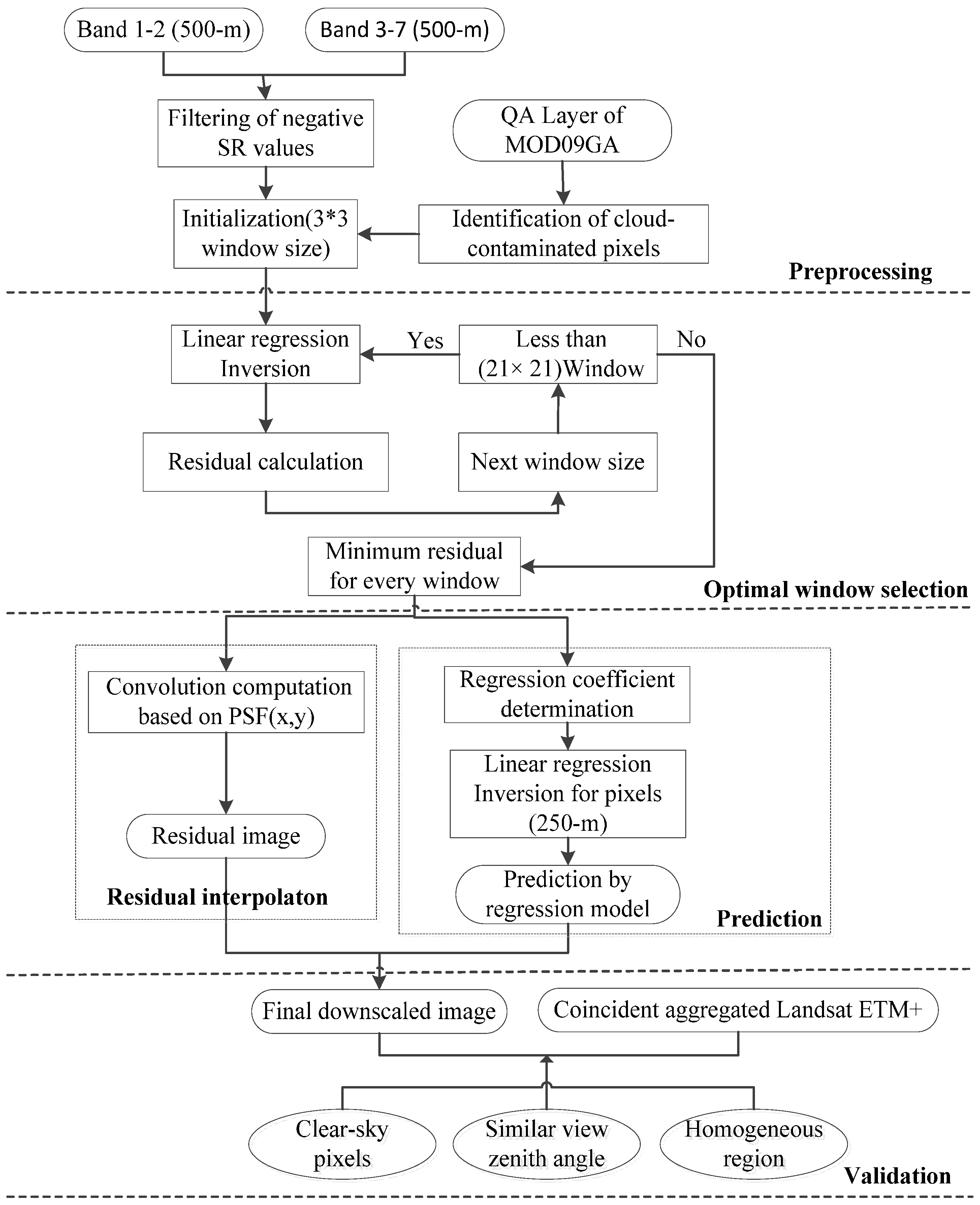
3.1. Downscaling Method

An improved version (i.e., IMAR) of MAR is proposed in the paper to predict SR values ( V i ( r , c ) ) at 250-m resolution for the four 500-m resolution spectral bands. IMAR includes two parts: regression ( V ˜ i ( r , c ) ) and residuals ( R i ( r , c ) ) based on point spread function (PSF). The method first performs regression of each coarser band to the finer band and then applies PSF to downscale the band residuals from the regression model. The prediction of IMAR is
V i ( r , c ) = V ˜ i ( r , c ) + R i ( r , c ) ,
where V ˜ i ( r , c ) and R i ( r , c ) are the predictions of the regression and residuals based on PSF parts, and r and c are row and column of pixels, respectively. The details regarding their calculation includes four steps: (1) linear regression using the correlation coefficient (CC) for each coarse band; (2) optimal window size selected by minimum residual; (3) spectral normalization based on PSF; and (4) calculation of each pixel’s reflectance and outputting of downscaled MODIS images by adding regression value and residual interpolation. The flowchart of the algorithm is shown in Figure 2.

3.1.1. Regression between Finer and Coarser Bands

In order to build regression model with quality-better pixels, a few negative SR values resulted from atmospheric correction algorithm were firstly filtered. In addition, cloud-contaminated pixels can also affect the accuracy of regression model. We exclude both cloud and shadow pixels from the regression data. Of the MODIS data, cloud and shadow are identified using the internal cloud and shadow masks from the MODIS QA band, which is a 16 bits band with 1 km spatial resolution. Two of the 16 bits are used to represent cloud state; one bit indicates cloud shadow status [25].
The regression part is presented as a linear function. The finer band to be fused for each coarse band is determined by using the spectral similarity between bands (in terms of correlation coefficient (CC)). MODIS band 1 has closer linear relationship with bands 3 and 4, while band 2 has similar correlation to bands 5, 6 and 7 [15]. Based on such linear correlation, a linear regression model is designed to estimate two coefficients for the j-th band at MODIS 500-m resolution. The regression prediction is calculated as
B j ( r , c ) = a i B i ( r , c ) + b i ,
where Bi is the observed reflectance for band i (i = 1 or 2) at coarser resolution; Bj is observed reflectance for band j (j = 3, 4, 6, 7); ai and bi are estimated by the linear model for the specific pixel; and r and c are row and column of specific pixel at 500-m resolution.
The key issue is the estimation of the two coefficients for the j-th band, that is, ai and bi. The relationship in Equation (2) is assumed to be universal at different spatial resolutions, and the relationship built at coarse spatial resolutions can be applied at fine spatial resolution [30]. Based on this hypothesis, Equation (3) holds
B j ( r / 2 , c / 2 ) = a i B i ( r / 2 , c / 2 ) + b i ,
where Bi is the observed reflectance for band i (i = 1 or 2) at 250-m resolution; Bj is corresponding predicted reflectance for band j (j = 3, 4, 6, 7); and r, c, ai and bi are derived from Equation (2).

3.1.2. Optimal Window (OW) Selection

To minimize the impact of vegetation diversity across different climatic and ecological zones, latitudinal variation of surface properties, and sun-view geometry effects on the SR prediction, the coefficients of regression model are estimated in a rectangular window centered to the MODIS target pixel. Owing to the different spatial distribution of each land cover class, the optimal window size s for each pixel, determined differently by minimum residual, ranges from rectangles of sizes of 3–21 MODIS pixels (0.15–10 km). Using the better-quality pixels within window length s, the built regression prediction is closest to the observed coarse value.
s = M i n { B j ( r , c ) [ a j , t B j ( r , c ) + b j , t ] } ,
where r and c are row and column of the MODIS target pixel at 500-m resolution; Bj is the observed SR value for band j (j = 3, 4, 6, 7); and t is the window size ranging from 3 to 21. Obviously, the size s of OW for the MODIS target pixel has the smallest residual. Thus, the window size s with the smallest residual was set to the size of OW for the MODIS target pixel.

3.1.3. Residuals Interpolation using PSF

The size of OW was determined to reduce bias between regression prediction and the observed coarse values. To the best of our knowledge, a perfect regression process does not exist without bias between prediction and the observed coarse band. As a result, any regression model can definitely lead to residuals. To honor the spectral properties, the residuals at coarser resolution should be interpolated to finer spatial resolution, which was taken as the second phase of downscaling method. In this paper, the residuals at finer spatial resolution were obtained by convolving residuals at the coarser resolution with the PSF adopted for MODIS (Equation (5)).
R ( x , y ) = P S F * r ( u , w ) = P S F ( x u , y w ) r ( u , w ) d u d w ,
where * denotes the convolution operator; x and y are coordinate offsets in relation to the center of the finer spatial pixel; u and w are coordinate offsets in relation to the center of the coarser spatial pixels within 5 × 5 window size centered on corresponding finer pixel; r (u, w) is the residual of coarser spatial pixel located at (u, w); and R (x, y) is the interpolated residual.
P S F ( x , y ) = k e x p ( x 2 + y 2 2 σ 2 ) ,
The PSF of a sensor dictates how the radiation over an area (specified by the locations x and y) and is integrated for generation of a pixel’s SR by the sensor. A two-dimensional Gaussian function is used for PSF. σhere is the spread parameter, which is usually set as the half of the pixel size; and k is sensor gain, which is usually set as 1 for MODIS sensor.

3.2. Water Detection Method

Numerous water detection methods from remotely sensed imagery have been explored, which can be divided into three categories: (1) the single-band threshold method based on spectral characteristic of lower near-infrared reflectivity [31,32,33]; (2) the multi-band spectral relationship method using logical judgment determined by the spectral difference between water and other land features [34,35,36]; (3) water index method by combining two or more spectral bands using various algebraic operations to enhance the discrepancy between water bodies and land [1,12,37,38]. It is impossible to determine a precise single-band threshold owing to different water quality, which makes the water index method widely used (especially MNDWI) to eliminate the difference between bands [6]. Water spectral reflectivity falls significantly since the wavelength of 0.6 um and the reflectivity of other land features obviously is higher than water, which makes the near-infrared or short-wave infrared bands suitable to detect water bodies. For the MODIS images, we can utilize bands 4 and 6 to extract water bodies by constructing Modified Normalized Difference Water Index (MNDWI) [13]. However, snow has similar reflectance difference as water, the TP2000 Lake Inventory dataset is applied to provide lake information and generate the lake seeds, which can expand water to lakes and remove noise [39].
M N D W I = C H 4 C H 6 C H 4 + C H 6 ,
where CH4 and CH6 are visible green and shortwave-infrared band reflectance in MODIS image, respectively. The threshold is set as 0.1, which is determined by visually comparing MODIS observations with water results extracted from different thresholds.

3.3. Trend and Season Decomposition Model

Detecting and characterizing lakes change over time is the natural first step toward identifying the driver of change and understanding the change mechanism. Therefore, in addition to some processes related to anthropogenic (e.g., deforestation, urbanization and farming) disturbances, phenological variability of lakes demonstrates the necessity of distinguishing long-term phenological change from temporal variability. A generic change detection approach for time series data is adopted, involving the detection and characterization of Breaks for Additive Seasonal and Trend (BFAST). BFAST integrates the decomposition of time series into trend, seasonal, and remainder components with methods for detecting and characterizing abrupt changes within the trend and seasonal components (Equation (8)) [40]. The trend component describes a gradual change in time-series variables at a time-scale longer than 1 year (which may include abrupt changes), indicating climate change and land development and management. The seasonal component is a regular and periodic change at an annual scale, primarily driven by the annual variation in insolation. The noise component is a stochastic and irregular variation that is caused by observation conditions (e.g., signal-to-noise ratio), atmospheric environments (e.g., clouds and aerosols) [41]. BFAST can be used to analyze different types of satellite image time series, and applied to other disciplines dealing with seasonal or non-seasonal time series, such as hydrology, climatology, and econometrics. In this paper, the algorithm is applied to lakes area, average monthly temperature (AMT) and precipitation (AMP).
Y t = T t + S t + e t   ( t   =   1 ,   ... ,   n ) ,
where Yt is the observed data at time t; Tt is the trend component; St is the seasonal component; and et is the remainder component. The remainder component is the remaining variation in the data beyond that in the seasonal and trend components.
Tt is described as a piecewise linear with segment-specific slopes and intercepts on m + 1 different segments, as given by Equation (9), which can extract the fundamental features of data and reduce the complexity of fitting curves [42].
T t = α i + β i t   ( τ i 1   <   t     τ i   and   i   =   1 ,   2 ,   ...   m ) ,
where τi is the position of the breakpoint; m is the total number of the breakpoints; and α i and β i are the slope and intercept of the linear function during each sub-period (τi−1 < t ≤ τi). The change magnitude is indicated by the slope. The breakpoint indicates an abrupt change that may be caused by abrupt changes in climate and anthropogenic impact.
Similarly, the seasonal component is fixed between breakpoints, but can vary across breakpoints. Here, a season harmonic model is used for the seasonal component represented by a widely-used sinusoidal function, as given by Equation (10).
S t = k = 1 K α j , k s i n ( 2 π k t f + δ j , k )   ( τ j 1   <   t     τ j   and   j   =   1 ,   2 ,   ...   p ) ,
where K is the number of harmonic terms; τj is the position of the breakpoints; and p is the total number of the breakpoints. The unknown parameters are the segment-specific season amplitude α j , k and phase δ j , k , which can be determined using an unconstrained Levenberg–Marquardt minimization with a universal optimization [43] on the detrended data; and f is the known frequency (e.g., f = 7 annual observations for lakes area, AMT and AMP time series).
The breakpoint number and breakpoint location in time sequence is needed to identify breakpoints of the trend and seasonal components. The ordinary least squares residuals-based moving sum (OLS-MOSUM) test is used to determine whether breakpoints occur in the time-series variables [42]. The optimal number and location of breakpoints is determined by minimizing the Bayesian information criterion and the sum of the regression residual squares, respectively, if the OLS-MOSUM test indicates significant structural changes (p < 0.05) [44]. In this study, we use BFAST package in R [45].

3.4. Accuracy Assessment

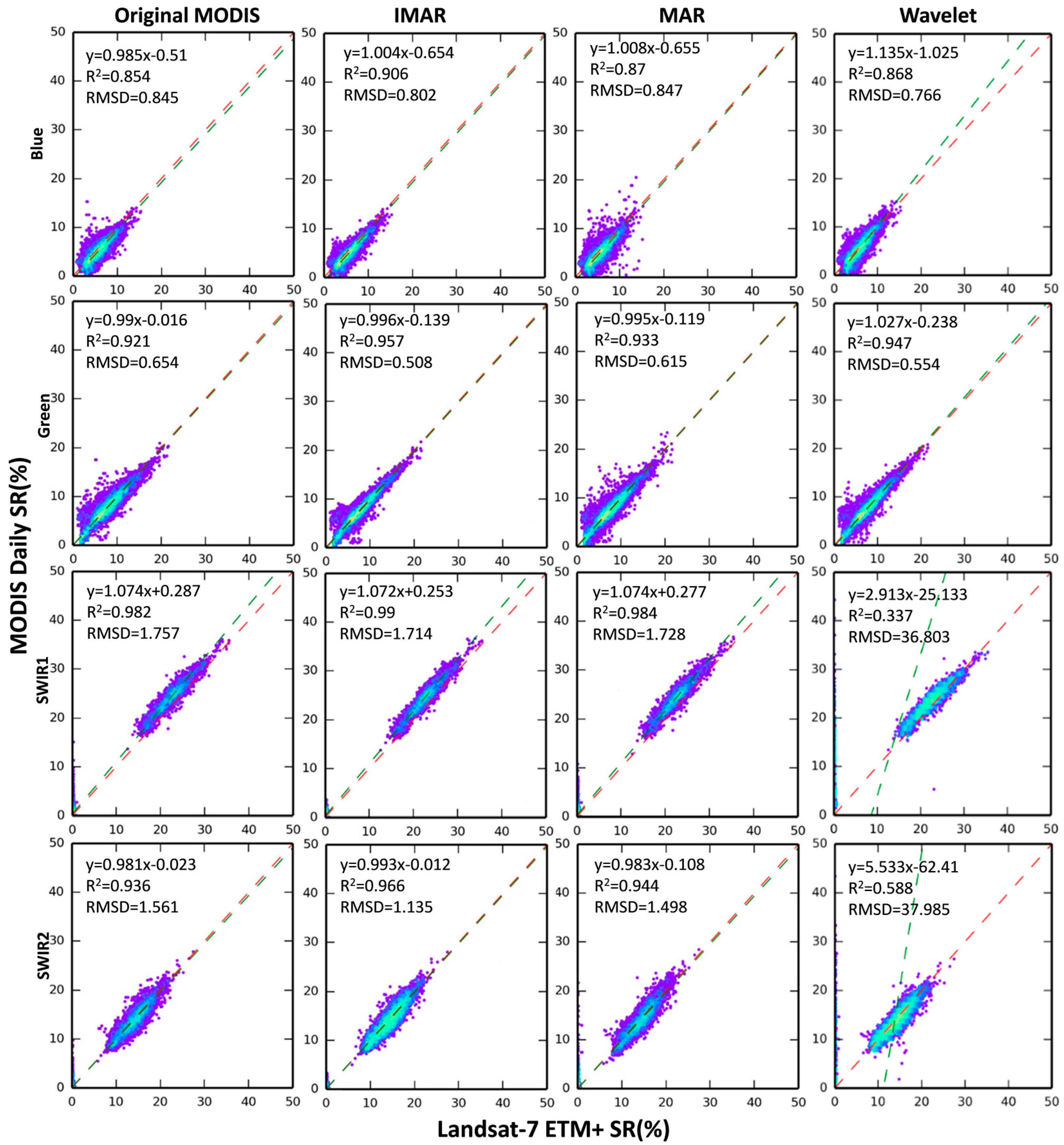
3.4.1. MODIS–Landsat-7 ETM+ SR Comparison

The Landsat-7 ETM+ image acquired on the same dates as MODIS data have been demonstrated to be qualified to validate the performance of downscaled SR [46]. Correlation and dependence index (R2) as well as Root Mean Square Deviation (RMSD) [6] were calculated to test the robustness of IMAR. Calculation of R2 and RMSD require ground footprints of the two sets of values match. Matching the footprints of Landsat and MODIS observations, however, can be complicated by several issues including data coordinate reference system (CRS), residual misregistration errors, sensor’s point spread function (PSF), adjacency effect, and view angle effect [47]. In order to minimize their impact on the agreement measures, these issues need to be addressed properly using the four processing steps:
(1)
To be comparable between Landsat and MODIS pixels, the image was aggregated to MODIS projection and pixel footprint.
(2)
Homogeneous regions at the Landsat and the MODIS resolutions were identified. Specifically, for the MODIS pixel, a value range is calculated as the difference between the maximum and the minimum values of the 9 MODIS pixels in the 3 × 3 window centered at that MODIS pixel. Similarly, the value range of all Landsat pixels located within a MODIS pixel coverage is also calculated. The MODIS pixels with two value ranges less than 0.03 were considered to be homogeneous.
(3)
To avoid the potential impact of different view zenith angles on the reflectance values (BRDF effect), only MODIS pixels having view zenith angles within the view zenith angle range of the Landsat (i.e., ±7.5° from nadir) were used in the comparison.
(4)
To minimize the impact due to cloud movement on the comparison results, both cloud and shadow pixels from MODIS and Landsat were excluded using MODIS QA band.

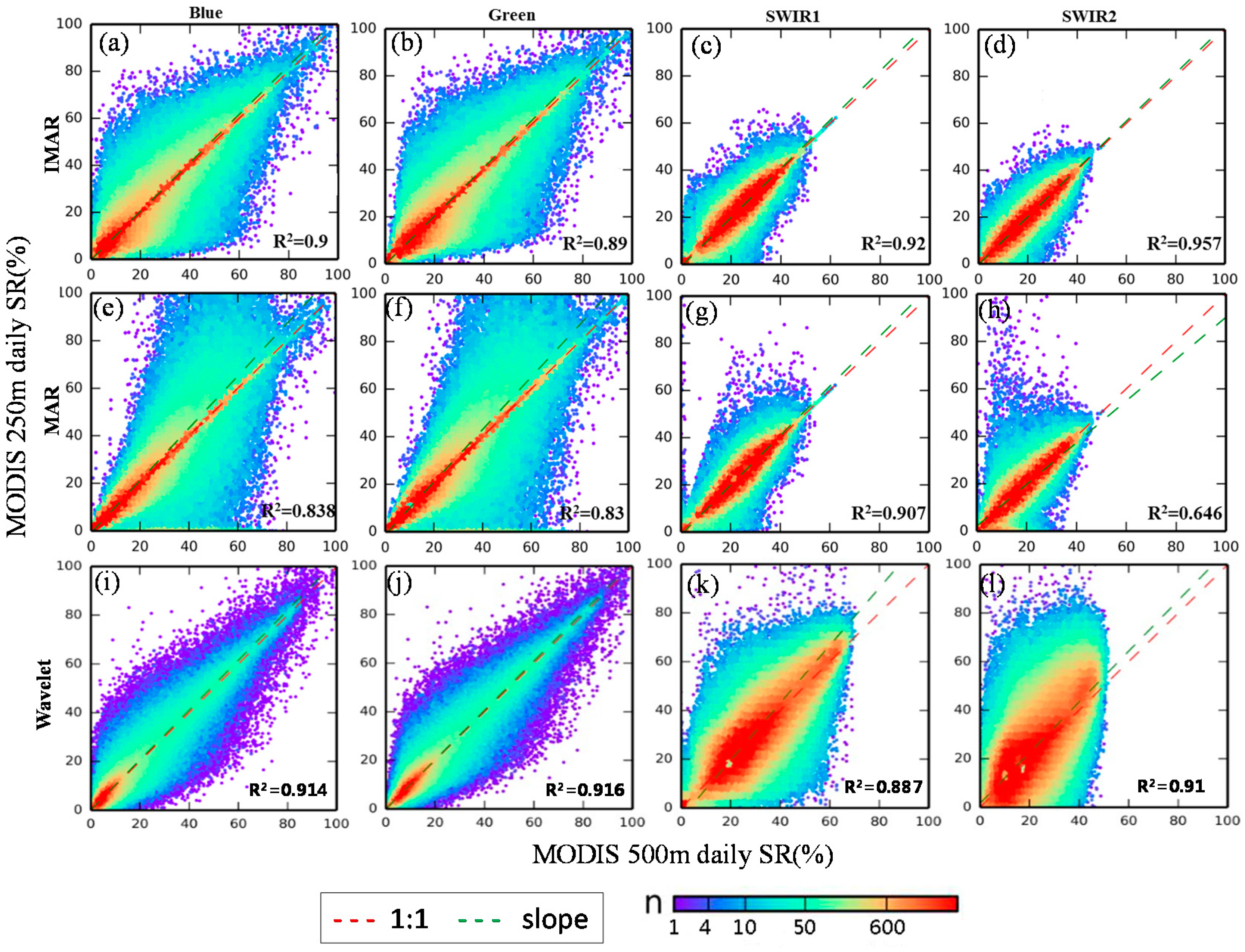
3.4.2. Spectral Fidelity Assessment

An important criterion for evaluation of the quality of fused images is the ability to conserve spectral properties (i.e., coherence). The SR from IMAR and MAR were compared to the original MODIS SR and coincidental Landsat-7 ETM+ SR to evaluate the consistency of IMAR. To match the spatial scale of the downscaled data, the original pixels were interpolated to 250-m resolution using Nearest Neighbor Interpolation (NNI). In addition, R2 and RMSD were calculated to measure the agreement and disagreement between the original and downscaled MODIS SR by building linear relationship between them.

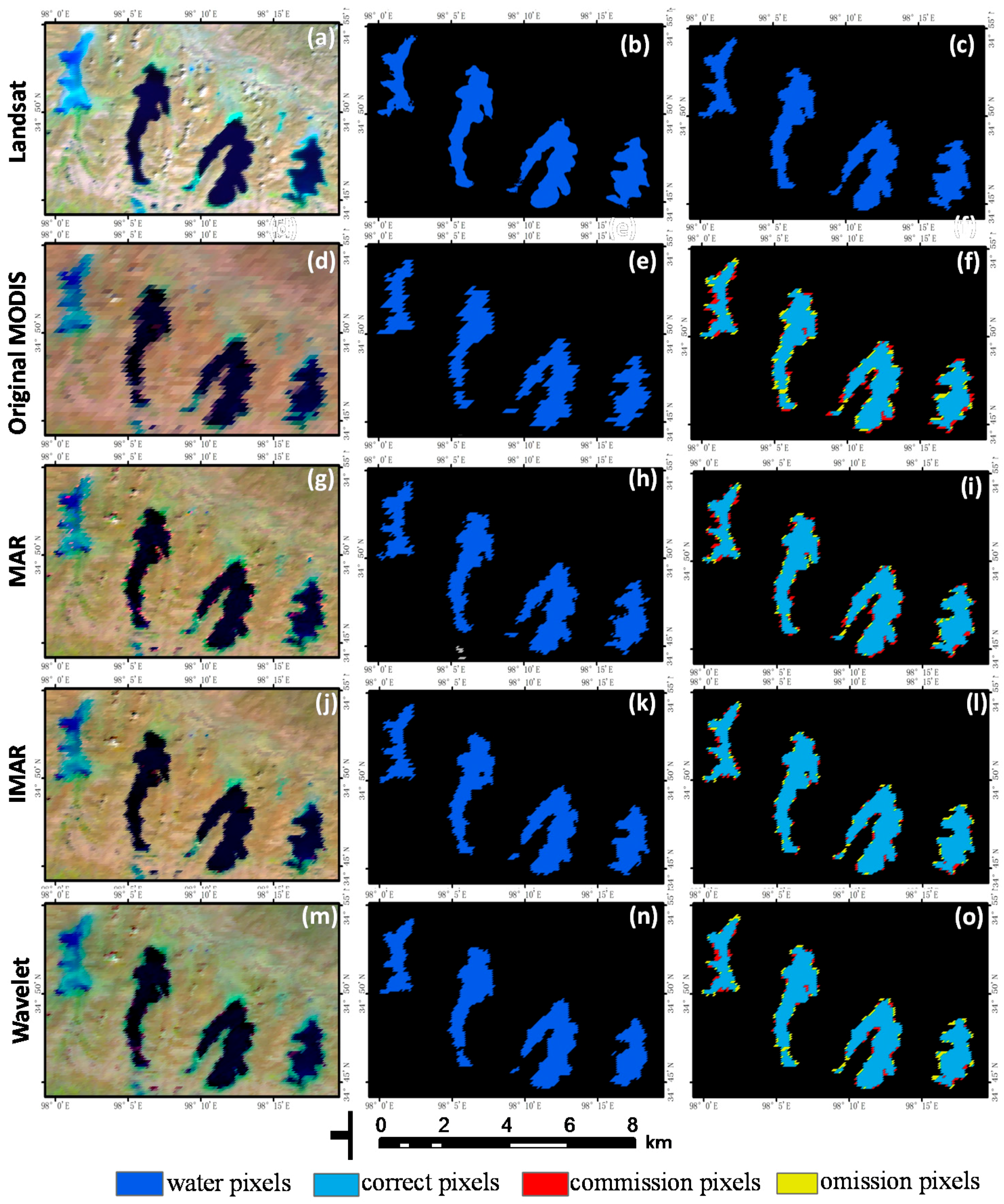
3.4.3. Water Classification Test on Fused Images

Water bodies identified from the original and downscaled MODIS SR images were compared to the water map manually interpreted from Landsat-7 ETM+ image for quality assessment. To match spatial resolution, water map produced from ETM+ image was aggregated to MODIS spatial resolutions using the principle of dominant method, which calculated the dominant majority type identified by ETM+ pixels located within the extent of each corresponding MODIS pixel. The aggregated water bodies were compared to the MODIS derived water maps. Confusion metrics were calculated to measures the accuracies—overall classification accuracy (OCA), and omission and commission errors (Eo and Ec, respectively) [6]. In addition, lakes morphometry measuring and analyzing lake dimensions was utilized to evaluate the accuracy of lake mapping from downscaled results. Five widely-used lake morphometry indexes were selected (maximum length and width, length of shoreline, shoreline development index and fractal dimension). Maximum length is the distance on the lake surface between the two most distant points on the lake shore while maximum width concerning lake productivity is the distance on the lake surface at a right angle to the line of maximum length on a lake. The length of shoreline refers to the perimeter of the lake [48]. Shoreline development index (DL) determining the trophic nature of a lake relates shoreline length to circumference of a circle that has the same area as the lake (Equation (11)). The fractal dimension (FD)—a measure of shape complexity of the perimeter of shoreline—was widely used in spatial and landscape pattern analysis and there are numerous related studies [33,49]. The fractal dimension of the lake can be derived mathematically from Equation (12) [50]. A “box dimension” method was used to calculate the fractal dimension. First, measure the quantities of the object under consideration using various box sizes. Second, plot log (measured quantities) versus log (box sizes) and fit a Least-squares regression line through the data points. The log–log plot is often referred to as the Richardson plot. Third, use the slope of the regression line to derive the fractal dimension of the lake.
D L = L 2 π r
where L is the length of the lake shoreline; and r is the radius of a circle of area equal to that of the lake.
F D = l o g ( N r ) l o g ( 1 / r )
where Nr represents an object of Nr parts scaled down by a ratio of r. The FD derived from Equation (12) is called fractal dimension. In this paper, r is different pixel sizes (1000, 500, 250, 50, 25, 5 and 1 m).

4. Results

4.1. Comparison of MODIS–Landsat-7 ETM+ SR

Figure 3 shows significant improvement of spatial delineation in IMAR result for the study area. For example, visually, the edges of lakes (Figure 3d) were showing closer areas and shapes to the higher resolution Landsat-7 ETM+ reference data (Figure 3a). The red pixels in the MAR result (Figure 3c) were fixed in IMAR result (Figure 3d). Although the downscaled composite (Figure 3e) from Wavelet fusion was more comparable spectrally to the Landsat-7 ETM+ composite (Figure 3a) compared to the result of IMAR (Figure 3d), some abnormal pixel values in the edge of lakes exist.
The performance of IMAR was further assessed qualitatively by comparing the MODIS and aggregated Landsat-7 ETM+ SR in density plots. As shown in Figure 4, the regression models between IMAR and aggregated Landsat-7 ETM+ SR (Figure 4) all have a closest 1:1 relationship for four bands, supported by their slopes of 1.004, 0.996, 1.072 and 0.993. R2 values of 0.906, 0.957, 0.99 and 0.966, and RMSD of 0.802, 0.508, 1.714 and 1.135. The comparison result between MAR and aggregated Landsat-7 ETM+ SR in Figure 4 was modeled by the slopes of 1.008, 0.995, 1.074 and 0.983, R2 values of 0.87, 0.933, 0.984 and 0.944, and RMSD of 0.847, 0.615, 1.728 and 1.498, respectively, which showed a slight improvement compared to original MODIS observations result (Figure 4) with the slopes of 0.985, 0.99, 1.074 and 0.981, R2 values of 0.854, 0.921, 0.982 and 0.936, and RMSD of 0.845, 0.654, 1.757 and 1.561, respectively. For the Wavelet fusion, the blue and green visible bands show a close link (R2 values of 0.868 and 0.947, and RMSD of 0.766 and 0.615) with Landsat SR while the R2 of two SWIR bands are less than 0.6. Figure 4 shows the regions with lower SR (mostly located on the water pixels) can lead to higher SR using Wavelet fusion, which limits the application of Wavelet fusion techniques to lake mapping. Obviously, the closer 1:1 relationship, the higher R2 and lower RMSD showed the greater performance of IMAR in image downscaling compared to the MAR and Wavelet results.

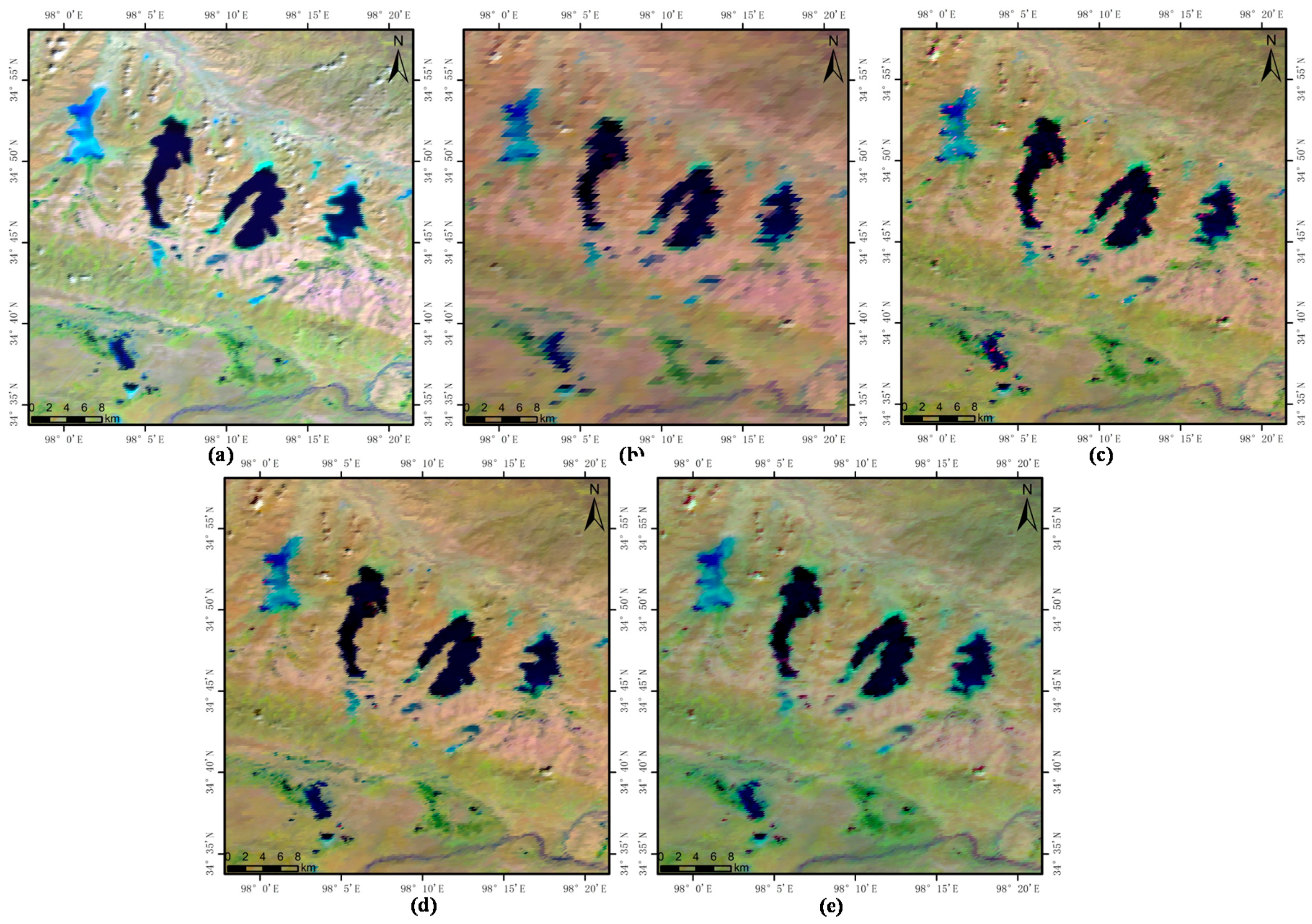
4.2. Fidelity of Downscaled MODIS SR

Considering the difference between downscaled and original composite image on spectral fidelity (Figure 3), the SR from IMAR, MAR and Wavelet fusion were compared to original MODIS SR. Figure 5 shows density plots of the three types of downscaled data for all four bands. As shown in Table 2, the R2 of IMAR for four bands increased to 0.919 compared to 0.805 of MAR, and the RMSD almost decreased by half to 2.585. Specifically, with higher R2 (0.9, 0.899, 0.92 and 0.957) and lower RMSD (3.225, 3.227, 2.098 and 1.79), four improved downscaled bands of IMAR have the higher correlation with the original coarser bands, especially for band 7 with R2 increasing from 0.646 to 0.957. R2 of MAR for all bands were less than 0.9 except for band 6 (0.907). The largest RMSD in MAR result is 4.737 for band 7 where there was the smallest RMSD (1.79) in IMAR, which indicated the obvious improvement for band 7 in terms of spectral fidelity. The higher scatter in two SWIR bands (Figure 5g–h) for MAR is primarily caused by excessive enhancement in the pixels of higher SR owing to the equally-weighted average method based on a 2 × 2 active window. In addition, the application of PSF with a two-dimensional Gaussian function make the downscaled result in IMAR closer to Landsat SR, which was especially apparent for blue and green visible bands. For Wavelet fusion, the R2 of blue and green bands (0.914 and 0.916) were slightly higher than IMAR results while the RMSD were higher (3.519 and 3.408) compared to IMAR results. Moreover, there were the largest deviations (4.46 and 6.339) on two SWIR bands, which indicated Wavelet fusion is not capable of preserving spectral fidelity of original MODIS observation.

4.3. Improvement of Water Classification on Fused Image

As shown in Figure 6, water maps derived from the proposed IMAR method had the highest consistency with the reference water map due to decreased commission (red pixels) and omission (yellow pixels) errors. The extracted lakes edges (Figure 6k) were smoother than the original MODIS observation (Figure 6e) and MAR results (Figure 6h), and closer to the Landsat result (Figure 6b). Even though lakes derived from Wavelet fusion held smoother shape (Figure 6n), the apparent omission errors can be found in Figure 6o. The quantitative subpixel accuracy assessment results are summarized in Table 3, where it is clear that the proposed IMAR method significantly outperforms the other three related methods, because only IMAR method had the ability to achieve higher OCA ranging from 90.12% to 94.95% for four lakes and lower average Ec of 7.13% and an average Eo of 6.65%. Water maps derived from original MODIS observation were the least accurate for four lakes. The highest OCA was 90.09% for Lake III while the lowest OCA only stood at 78.23% for Lake IV. The OCA (fluctuating from 88.54% to 93.51%) of MAR for four lakes still were lower compared to the IMAR results. In addition, for Lake II, even if the lake area of MAR (25.92 km2) is closer to reference area (25.973 km2) compared to 25.705 km2 of IMAR, the Eo and Ec were higher than that of IMAR. In terms of water errors from Wavelet fusion, the obvious omission errors can be found ranging from 6.85% to 11.46%, which indicated Wavelet fusion can underestimate water surface in general. The highest OCA was 93.15% for Lake III, while the lowest OCA was 87.54% for Lake IV. The greater Ec and smaller Eo were observed for original observation and MAR results, suggesting that the overall water surface is over-estimated. Additionally, the linear models for lake areas were built between downscaled results and the high resolution Landsat-7 ETM+ reference data. R2 for IMAR is the highest (0.9993), and lowest R2 is 0.9699 for original MODIS. The R2 for MAR and Wavelet is 0.985 and 0.9887, respectively. These results reveal the great potential of IMAR applied to MODIS data for small lakes monitoring.
In addition to Eo, Ec and OCA, five widely-used lake morphometry indexes (maximum length and width, length of shoreline, shoreline development index and fractal dimension) also showed IMAR held the better performance compared to MAR and Wavelet fusion. For every lake morphometry index, the result from IMAR achieved the closest values to the Landsat ETM+ (Figure 7). On average, compared to the shoreline lengths from Landsat for four lakes (50.04 km), the lengths from IMAR were 49.63 km while the largest deviation was from MAR (54.44 km). The maximum length and width of lakes was 12.626 km and 3.475 km for Landsat, and closest lengths and width to Landsat were 12.629 km and 3.417 km from IMAR while the length and width of lakes from Wavelet fusion were smallest and only stood at 11.466 and 3.23 km. This result also indicated Wavelet fusion can lead to obvious underestimate of lake distribution, which was consistent with the pattern of lake area extraction of Wavelet fusion. The shoreline development indexes for Landsat and IMAR almost were the same (3.064), whereas the index from Wavelet fusion was only 2.731. In terms of fractal dimension, the index was 2.0019 for Landsat, but the original MODIS observation reached the largest value of 2.0135 among other downscaled methods.

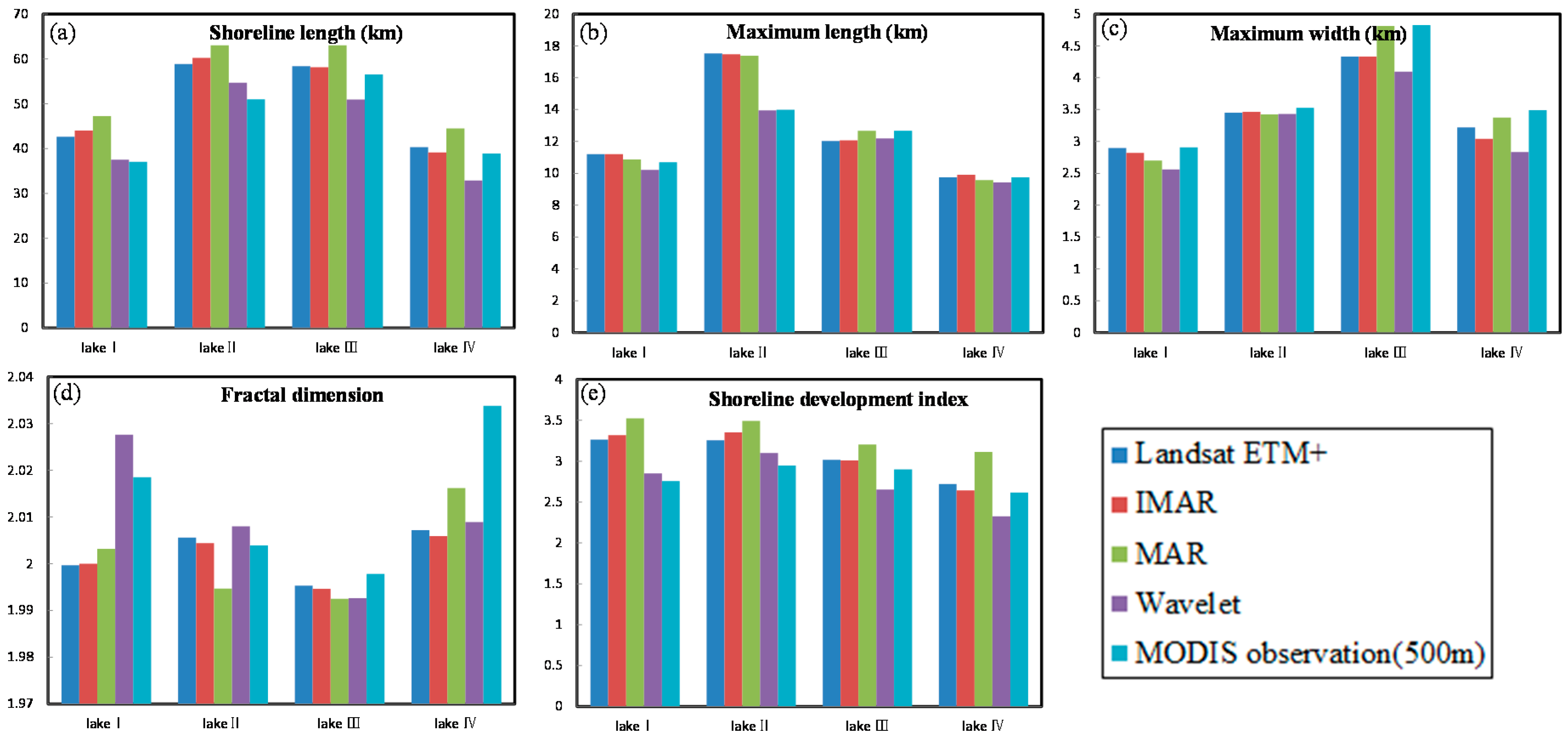
4.4. Lake Dynamics Trend

The downscaled and water detection methods are applied to all 190 MODIS tiles to estimate lake dynamics over the period between 2000 and 2014 at 250-m resolution. Considering the lakes in the TP have long frozen and snow covering period, we only analyze lake extents identified from May to November. To remove random noises, for each month in specific year, there may be several lake layers, which can be integrated to the monthly water mapping using the majority principle. The detected water extents of the four lakes from 2000 to 2014 were decomposed to fitted seasonal, trend and remainder components (Figure 8). For the fitted trend components, the area of three lakes except for Lake II experienced a gradual increase since circa 2005, while there was a continuous decrease from 2000 to circa-2005. The fitted seasonal trend indicates four lakes dynamics is closely related to the seasonality.
Specifically, Lake I had the smallest area (4.907 km2) in 2005 and the decreasing rate was nearly 3.12 km2/10a. However, there was a reverse trend since June 2005 (detected breakpoint), and the increasing rate was 13.08 km2/10a. Lake II showed a continuous increasing trend (7.08 km2/10a), and there was no breakpoint detected during 15 years. Obviously, the area of Lake III showed the similar trend as Lake I, and the decreasing rate and increasing rate was 1.8 km2/10a and 9.36 km2/10a, respectively. There were two breakpoints for Lake III. Conversely, there was a complicated variation for Lake IV. The area declined to 8.369 km2 in 2005 with the decreasing rate of 29.04 km2/10a, and then started to increase continuously until 2008 with the largest increasing rate of 31.8 km2/10a, and ended with a smallest decreasing rate of 1.2 km2/10a.
In terms of the seasonal component, the variation pattern of lakes area indicates the obvious seasonality. Lake I and Lake II had higher seasonal amplitudes (−3–1) in comparison to Lake III and Lake IV (−2–1), which implies the former lakes changed more significantly during the specific year.

5. Discussion

5.1. Usability of CC, OW, PSF for Downscaling Method

In this paper, when building regression model in IMAR, three factors were considered. First, the valuable fine spatial resolution texture information should be used efficiently. In theory, both bands 1 and 2 can be used for building the relation between fine and coarse bands, which involves multivariate regression. However, using all fine bands as covariates does not necessarily lead to an improvement in the prediction. Some variables may have small correlations limiting the ability of providing useful fine spatial resolution information. In MAR, based on the non-linear correlation between MODIS B3 to B7 and B1, B2 and NDVI, a regression model was designed to calculate regression parameters for 500 m resolution, which was then applied to MODIS 250 m B1 and B2 to predict corresponding B3-7 SR [6]. Redundancy in B1, B2 and NDVI led to the higher scatter of two visible bands (Figure 4). In this paper, one fine band is selected from bands 1 and 2. The CC (R2 and RMSD) of seven bands for MODIS data has been investigated widely, which were used to explore the possible correlation between MODIS bands [15,51]. Therefore, based on the CC of spectral similarity between MODIS bands, only the fine band with strongest CC was determined as the one spectrally closest to the coarse band. According this scheme for fine band selection, a fine band from bands 1 and 2 for each coarse band of bands 3–7 was determined as the one spectrally closest to the coarse band. The simple linear relationship, on the one hand, can maintain the similar correlation between MODIS bands, which can be demonstrated from Figure 3. The higher scatter in MAR was reduced in IMAR. On the other hand, model building helped to boost computation efficiency. Second, the calculation of regression coefficient required pixel subset within similar natural condition (e.g., similar climatic and ecological zones, vegetation type, geolocation and sun-view geometry effects). Wang et al. [17] used one set of regression coefficient for the entire MODIS tile. Small sub-regions and classification of each region were also explored by Trishchenko et al. [52] to build non-linear regression model for every vegetation type, which indicated complex land cover classification, and even the same vegetation type cannot guarantee the spectral similarity owe to larger geolocation deviation. Instead, Che et al. [6] utilized NDVI segmentation as regression unit to derive the regression coefficient, but some outliers existed at the transition boundary of different land covers (Figure 3c), which was primarily caused by the regression model built using pixels located in the heterogeneous regions. In this paper, each pixel had a specific OW determined by the minimum residual, which facilitated identifying the similar pixels to precisely calculate the coefficients of regression model for the target pixel. Third, even though efforts were made to improve the performance of regression model, there were still some residuals. It is another significant advantage of IMAR to precisely preserve spectral properties of the coarse data with PSF to eliminate the residuals. The PSF effect exists in remote sensing images, which indicates the pixel value in coarse images is derived from a convolution of fine pixel values within the particular extent centered at the corresponding pixel at 500 m [53]. Some previous study tended to use a simple 2 × 2 pass filter to ensure that any substantial mismatch between regression results and original 500 m MODIS imagery was removed [6,54]. For mixed pixels at 500 m resolution at the edge of the lakes, SR values of the corresponding four pixels at 250 m change greatly, especially in the two MODIS SWIR bands (Figure 3). As a result, the equally-weighted average method with a simple 2 × 2 pass filter in MAR generally caused excessive enhancement in the pixels of higher SR and widened the distinction among neighboring pixels. This error tends to have higher SR values than the original MODIS observation (Figure 5g–h). In IMAR, a two-dimensional Gaussian function is used for PSF calculation considering the target pixel radiation derived from the neighboring pixels with different Euclidean distance-based weights, which made it possible to preserve the spectral fidelity because this PSF calculation incorporated more information from coarse data. On the whole, the regression part of IMAR took advantage of fine spatial resolution information from fine bands, while the PSF part downscale residuals by considering the spatial correlation between the coarse pixels in the observed coarse bands. The two parts were complementary. The regression part helped to derive coherence of the coarse data, while using the PSF part can restore the high frequency details mainly encapsulated in boundaries and heterogeneous texture.
On the other hand, although we used CC, OW, PSF to improve the accuracy of downscaling method, these still exists be some problems. For example, the systematic errors between MODIS and Landsat cannot be removed efficiently when comparing, which can be found in Figure 4, especially for two SWIR bands. The much narrower bandwidths of the two MODIS SWIR bands made it possible to avoid the spectral ranges with lower atmospheric transmittance that were covered by the Landsat SWIR bands [47]. As a result, most MODIS SR values were higher than the Landsat values in those two bands (Figure 4), and the SWIR bands had higher RMSD values than the other 2 bands, which may be another important research of using MODIS and Landsat data in the near future.

5.2. Analysis of Lake Dynamics

As shown in Figure 8, except for Lake II showing a steady increase, the area of other three lakes fluctuated, and breakpoints were detected. For Lake I, BFAST detected the breakpoint on June 2005, and a slight decrease before 2005 and an increase after 2005 is consistent with the lake dynamic trend explored by Duan et al. using the Landsat data [55]. For Lake III, the breakpoint existed on November 2002, primarily caused by the discontinuity of lakes data from November 2002 to May 2003. For Lake IV, the first breakpoint was identified on November 2004 probably resulted from the discontinuity of lakes data from November 2004 to May 2005, while the abrupt change in 2008 is likely due to a large-scale continuous precipitation between 15–19 June 2007 [56], which is also consistent with the results by Duan et al. [55].
Variations in temperature and precipitation strongly affect lakes and glaciers by influencing the hydrological cycle and water phase variability [57]. Around four lakes, there is a Madoi meteorological station (Figure 1), and the temperature and precipitation change were analyzed to explored lakes dynamics. Figure 9 shows from 2000 to 2014, the average temperature experienced a gradual increase, and increasing rate was about 0.372 °C/10a, and the increasing rate of precipitation was approximately 5.136 mm/10a, which showed similar tendency as water surface dynamics of Lake II. Meantime, the correlations between lakes area and meteorological variables are analyzed quantitatively at monthly scale, which can be identified using Pearson correlation coefficient (R2) [58]. Table 4 indicates lakes dynamics has a strong correlation with the variation of temperature (0.598–0.728) and precipitation (0.61–0.735), especially for Lake II with the highest R2 of more than 0.7 for two variables. This correlation indicated a potential indicator of climate change of study area using the surface variation of Lake II, while the other three lakes with lower R2 were inappropriate to indicate climate change. Additionally, without the decomposing process based on BFAST, the R2 only ranges from 0.159 to 0.295, which cannot accurately identify the close relationship between lakes area and temperature and precipitation. The results also indicated the BFAST is appropriate and robust for change analysis in various situations, including lake area dynamics and the meteorological variables change.
Lake surface dynamics were affected by many factors such as the structure of lakes, surrounding topography, hydrological processes (e.g., inflows and outflows, and evaporation capacity) [59]. Up to now, little research is concentrated on these lakes of small size, which makes it difficult to comprehensively analyze the lake surface dynamic using adequate auxiliary data. This indicates that the lake dynamics is more complicated and requires further research for exploring the driver of lakes variations.

6. Conclusions

Considering the limitations in MAR, this paper presented an improved downscaling method, called IMAR for MODIS image. It fuses coarse bands 3–7 with fine bands 1 and 2, which consists of regression modeling and residuals interpolation using PSF. The performance of IMAR is proven to be excellent when comparing with original MODIS, MAR and Wavelet fusion. Meanwhile, the ability of IMAR to improve the extraction of water bodies was tested on four lakes (Longre Co, Ayonggongma Co, Ayonggama Co, and Ayongwama Co) in the TP. The smoother edge of lakes, smaller commission and omission errors and closest lake morphometry indexes to that of Landsat ETM+ show the improvement over the original downscaled data in terms of downscaled SR and water classification. When analyzing lakes dynamics, BFAST is used to decompose time series into trend, seasonal, and remainder components. It is found that four lakes change indicate obvious seasonality, and experience a continuous expansion trend after circa-2005. The relationship between lakes area and meteorological variables (temperature and precipitation) was analyzed using BFAST. The higher R2 demonstrates the lakes dynamics is directly related to the temperature and precipitation variation and indicates a potential indicator of climate change of study area using the surface variation of Lake II, which also has proven the robustness of BFAST in decomposing trend and season time-series.

Acknowledgments

This research was supported by the Geographic Resources and Ecology Knowledge Service System of China Knowledge Center for Engineering Sciences and Technology (No. CKCEST-2015-1-4), the National Special Program on Basic Science and Technology Research of China (No. 2013FY110900), National Science Foundation (No. 41501117), and the National Data Sharing Infrastructure of Earth System Science. The authors are indebted to the National Aeronautics and Space Administration for providing the MODIS data and U.S. Geological Survey server that were used in this study. We also thank the National Data Sharing Infrastructure of Earth System Science for providing the lake data of China. In addition, we would like to thank the anonymous reviewers for their helpful comments and suggestions in enhancing this manuscript.

Author Contributions

Xianghong Che drafted the manuscript and was responsible for the research design, experiment, and analysis. Yaping Yang reviewed the manuscript and was responsible for the research design and analysis. Tong Xiao, Min Feng and Shengli Huang provided some of the data and gave relevant technical support. Yang Xiang and Zugang Chen supported the data preparation and the interpretation of the results. All of the authors contributed to editing and reviewing the manuscript.

Conflicts of Interest

The authors declare no conflict of interest.

References

  1. Feyisa, G.L.; Meilby, H.; Fensholt, R.; Proud, S.R. Automated water extraction index: A new technique for surface water mapping using Landsat imagery. Remote Sens. Environ. 2014, 140, 23–35. [Google Scholar] [CrossRef]
  2. Downing, J.A. Emerging global role of small lakes and ponds: Little things mean a lot. Limnetica 2010, 29, 9–24. [Google Scholar]
  3. Liu, C.; Xian, D.; Quan, J. The change of effectively irrigated land area in China during the past 20 years. Resour. Sci. 2006, 28, 8–12. [Google Scholar]
  4. Huang, Z.; Xue, B.; Yao, S.; Pang, Y. Lake evolution and its implication for environmental changes in China during 1950–2000. J. Geogr. Sci. 2008, 18, 131–141. [Google Scholar] [CrossRef]
  5. Cammalleri, C.; Ciraolo, G.; Minacapilli, M.; Rallo, G. Evapotranspiration from an olive orchard using remote sensing-based dual crop coefficient approach. Water Resour. Manag. 2013, 27, 4877–4895. [Google Scholar] [CrossRef]
  6. Che, X.; Feng, M.; Jiang, H.; Song, J.; Jia, B. Downscaling MODIS surface reflectance to improve water body extraction. Adv. Meteorol. 2015. [Google Scholar] [CrossRef]
  7. Jain, S.K.; Singh, R.; Jain, M.; Lohani, A. Delineation of flood-prone areas using remote sensing techniques. Water Resour. Manag. 2005, 19, 333–347. [Google Scholar] [CrossRef]
  8. Frazier, P.S.; Page, K.J. Water body detection and delineation with Landsat TM data. Photogramm. Eng. Remote Sens. 2000, 66, 1461–1468. [Google Scholar]
  9. Smith, L.C. Satellite remote sensing of river inundation area, stage, and discharge: A review. Hydrol. Process. 1997, 11, 1427–1439. [Google Scholar] [CrossRef]
  10. Sun, F.; Zhao, Y.; Gong, P.; Ma, R.; Dai, Y. Monitoring dynamic changes of global land cover types: Fluctuations of major lakes in China every 8 days during 2000–2010. Chin. Sci. Bull. 2014, 59, 171–189. [Google Scholar] [CrossRef]
  11. Vikhamar, D.; Solberg, R. Snow-cover mapping in forests by constrained linear spectral unmixing of MODIS data. Remote Sens. Environ. 2003, 88, 309–323. [Google Scholar] [CrossRef]
  12. McFeeters, S.K. The use of the normalized difference water index (NDWI) in the delineation of open water features. Int. J. Remote Sens. 1996, 17, 1425–1432. [Google Scholar] [CrossRef]
  13. Xu, H. Modification of normalised difference water index (NDWI) to enhance open water features in remotely sensed imagery. Int. J. Remote Sens. 2006, 27, 3025–3033. [Google Scholar] [CrossRef]
  14. Ji, L.; Zhang, L.; Wylie, B. Analysis of dynamic thresholds for the normalized difference water index. Photogramm. Eng. Remote Sens. 2009, 75, 1307–1317. [Google Scholar] [CrossRef]
  15. Kim, S.-H.; Kang, S.-J.; Lee, K.-S. Comparison of fusion methods for generating 250 m MODIS image. Korean J. Remote Sens. 2010, 26, 305–316. [Google Scholar]
  16. Ribeiro Sales, M.H.; Souza, C.M.; Kyriakidis, P.C. Fusion of MODIS images using kriging with external drift. IEEE Trans. Geosci. Remote Sens. 2013, 51, 2250–2259. [Google Scholar] [CrossRef]
  17. Wang, Q.; Shi, W.; Atkinson, P.M.; Zhao, Y. Downscaling MODIS images with area-to-point regression kriging. Remote Sens. Environ. 2015, 166, 191–204. [Google Scholar] [CrossRef]
  18. Ma, R.; Yang, G.; Duan, H.; Jiang, J.; Wang, S.; Feng, X.; Li, A.; Kong, F.; Xue, B.; Wu, J. China’s lakes at present: Number, area and spatial distribution. Sci. China Earth Sci. 2011, 54, 283–289. [Google Scholar] [CrossRef]
  19. Aiazzi, B.; Alparone, L.; Baronti, S.; Garzelli, A. Context-driven fusion of high spatial and spectral resolution images based on oversampled multiresolution analysis. IEEE Trans. Geosci. Remote Sens. 2002, 40, 2300–2312. [Google Scholar] [CrossRef]
  20. Zhang, S.; Shao, Q.; Liu, J.; Xu, X. Land use and landscape pattern change in Madoi County, the source region of Yellow River. Geo-Inf. Sci. 2007, 4, 021. [Google Scholar]
  21. Wang, S.; Dou, H. Chinese Lakes; Science Press: Beijing, China, 1998; p. 5. [Google Scholar]
  22. Wan, L.; Cao, W.; Zhou, X.; Hu, F.; Li, Z.; Xu, W. Changes of the water environment in the headwater area of the Yellow River and the cause for the zero-flow of the river occurring in winter. Geol. Bull. China 2003, 22, 521–526. (In Chinese) [Google Scholar]
  23. The National Disaster Monthly Report. Disaster Reduction in China; National Disaster Reduction Center: Beijing, China, 2007; pp. 54–63.
  24. Salomonson, V.V.; Barnes, W.; Maymon, P.W.; Montgomery, H.E.; Ostrow, H. Modis: Advanced facility instrument for studies of the earth as a system. IEEE Trans. Geosci. Remote Sens. 1989, 27, 145–153. [Google Scholar] [CrossRef]
  25. Vermote, E.; Kotchenova, S.; Ray, J. Modis Surface Reflectance User’s Guide; MODIS Land Surface Reflectance Science Computing Facility; Terrestrial Information Systems Laboratory: Maryland, MD, USA, 2008; p. 1. [Google Scholar]
  26. MODIS. Available online: http://modis.gsfc.nasa.gov (accessed on 7 October 2016).
  27. Vermote, E.F.; El Saleous, N.Z.; Justice, C.O. Atmospheric correction of MODIS data in the visible to middle infrared: First results. Remote Sens. Environ. 2002, 83, 97–111. [Google Scholar] [CrossRef]
  28. Global Land Cover Facility. Available online: http://www.landcover.org/data/gls_SR (accessed on 10 October 2016).
  29. Masek, J.G.; Vermote, E.F.; Saleous, N.E.; Wolfe, R.; Hall, F.G.; Huemmrich, K.F.; Gao, F.; Kutler, J.; Lim, T.-K. A Landsat surface reflectance dataset for North America, 1990–2000. IEEE Geosci. Remote Sens. Lett. 2006, 3, 68–72. [Google Scholar] [CrossRef]
  30. Gao, F.; Masek, J.G.; Wolfe, R.E.; Huang, C. Building a consistent medium resolution satellite data set using moderate resolution imaging spectroradiometer products as reference. J. Appl. Remote Sens. 2010, 4, 043526. [Google Scholar]
  31. Zheng, W.; Shao, J.; Wang, M.; Huang, D. A thin cloud removal method from remote sensing image for water body identification. Chin. Geogr. Sci. 2013, 23, 460–469. [Google Scholar] [CrossRef]
  32. Lu, J.; Li, S. Improvement of the techniques for distinguishing water bodies from TM data. Remote Sens. Environ. 1992, 7, 17–23. [Google Scholar]
  33. Ovakoglou, G.; Alexandridis, T.K.; Crisman, T.L.; Skoulikaris, C.; Vergos, G.S. Use of MODIS satellite images for detailed lake morphometry: Application to basins with large water level fluctuations. Int. J. Appl. Earth Obs. Geo-Inf. 2016, 51, 37–46. [Google Scholar] [CrossRef]
  34. Li, X.-M.; Wang, G.; Tian, J. Study of the method of picking-up small water-bodies in Landsat TM remote sensing image. J. Southwest Agric. Univ. 2006, 4, 15. [Google Scholar]
  35. Ding, L.; Wu, H.; Wang, C.; Qin, Z.; Zhang, Q. Study of the water body extracting from MODIS images based on spectrum-photometric method. Geomat. Spat. Inf. Technol. 2006, 29, 25–27. [Google Scholar]
  36. Zhou, C.; Luo, J.; Yang, X.; Yang, C. Geo-Understanding and Analysis in Remote Sensing Image; Science Press: Beijing, China, 2003. [Google Scholar]
  37. Xu, H. A study on information extraction of water body with the modified normalized difference water index (MNDWI). J. Remote Sens. 2005, 5, 589–595. [Google Scholar]
  38. Hu, C.; Lee, Z.; Ma, R.; Yu, K.; Li, D.; Shang, S. Moderate resolution imaging spectroradiometer (MODIS) observations of cyanobacteria blooms in Taihu Lake, China. J. Geophys. Res. Oceans 2010, 115. [Google Scholar] [CrossRef]
  39. Jiang, H.; Feng, M.; Zhu, Y.; Lu, N.; Huang, J.; Xiao, T. An automated method for extracting rivers and lakes from Landsat imagery. Remote Sens. 2014, 6, 5067–5089. [Google Scholar] [CrossRef]
  40. Verbesselt, J.; Zeileis, A.; Hyndman, R.; Verbesselt, M.J. Package ‘bfast’. 2012. Available online: https://cran.r-project.org/web/packages/bfast/bfast.pdf (accessed on 16 January 2017).
  41. Quan, J.; Zhan, W.; Chen, Y.; Wang, M.; Wang, J. Time series decomposition of remotely sensed land surface temperature and investigation of trends and seasonal variations in surface urban heat islands. J. Geophys. Res. Atmos. 2016, 121, 2638–2657. [Google Scholar] [CrossRef]
  42. Zeileis, A.; Kleiber, C.; Krämer, W.; Hornik, K. Testing and dating of structural changes in practice. Comput. Stat. Data Anal. 2003, 44, 109–123. [Google Scholar] [CrossRef]
  43. Göttsche, F.-M.; Olesen, F.S. Modelling of diurnal cycles of brightness temperature extracted from METEOSAT data. Remote Sens. Environ. 2001, 76, 337–348. [Google Scholar] [CrossRef]
  44. Zeileis, A.; Leisch, F.; Hornik, K.; Kleiber, C. Strucchange. An R Package for Testing for Structural Change in Linear Regression Models; WU Vienna University of Economics and Business: Vienna, Austria, 2001. [Google Scholar]
  45. Verbesselt, J.; Hyndman, R.; Zeileis, A.; Culvenor, D. Phenological change detection while accounting for abrupt and gradual trends in satellite image time series. Remote Sens. Environ. 2010, 114, 2970–2980. [Google Scholar] [CrossRef]
  46. Roy, D.P.; Ju, J.; Lewis, P.; Schaaf, C.; Gao, F.; Hansen, M.; Lindquist, E. Multi-temporal MODIS–Landsat data fusion for relative radiometric normalization, gap filling, and prediction of Landsat data. Remote Sens. Environ. 2008, 112, 3112–3130. [Google Scholar] [CrossRef]
  47. Feng, M.; Huang, C.; Channan, S.; Vermote, E.F.; Masek, J.G.; Townshend, J.R. Quality assessment of Landsat surface reflectance products using MODIS data. Comput. Geosci. 2012, 38, 9–22. [Google Scholar] [CrossRef]
  48. Hakanson, L. A Manual of Lake Morphometry; Springer Science & Business Media: Berlin/Heidelberg, Germany, 2012. [Google Scholar]
  49. Thomas, I.; Frankhauser, P.; Biernacki, C. The morphology of built-up landscapes in Wallonia (Belgium): A classification using fractal indices. Landsc. Urban Plan. 2008, 84, 99–115. [Google Scholar] [CrossRef]
  50. Sun, W.; Xu, G.; Gong, P.; Liang, S. Fractal analysis of remotely sensed images: A review of methods and applications. Int. J. Remote Sens. 2006, 27, 4963–4990. [Google Scholar] [CrossRef]
  51. Sirguey, P.; Mathieu, R.; Arnaud, Y.; Khan, M.M.; Chanussot, J. Improving MODIS spatial resolution for snow mapping using wavelet fusion and ARSIS concept. IEEE Geosci. Remote Sens. Lett. 2008, 5, 78–82. [Google Scholar] [CrossRef] [Green Version]
  52. Trishchenko, A.P.; Luo, Y.; Khlopenkov, K.V. A Method for Downscaling Modis Land Channels to 250 m Spatial Resolution Using Adaptive Regression and Normalization Alexander; SPIE: Bellingham, WA, USA, 2006; Volume 6366. [Google Scholar]
  53. Van der Meer, F. Remote-sensing image analysis and geostatistics. Int. J. Remote Sens. 2012, 33, 5644–5676. [Google Scholar] [CrossRef]
  54. Trishchenko, A.P.; Luo, Y.; Khlopenkov, K.V.; Wang, S. A method to derive the multispectral surface albedo consistent with MODIS from historical ANHRR and VGT satellite data. J. Appl. Meteorol. Climatol. 2008, 47, 1199–1221. [Google Scholar] [CrossRef]
  55. Duan, S.; Fan, S.; Cao, G.; Liu, X.; Sun, Y. The changing features and cause analysis of the lakes in the source regions of the Yellow River from 1976 to 2014. J. Glaciol. Geocryol. 2015, 37, 745–756. [Google Scholar]
  56. Che, X.; Feng, M.; Jiang, H. Detection and Analysis of Qinghai-Tibet Plateau Lake Areas from 2000 to 2013. J. Geo-Inf. Sci. 2015, 17, 99–107. [Google Scholar]
  57. Qin, B.; Shi, Y.; Yu, G. Lake level fluctuations of Asia inland lakes during 18 kaBP and 6 kaBP with their significance. Chin. Sci. Bull. 1997, 42, 2586–2595. [Google Scholar]
  58. Zou, K.H.; Tuncali, K.; Silverman, S.G. Correlation and simple linear regression 1. Radiology 2003, 227, 617–628. [Google Scholar] [CrossRef] [PubMed]
  59. Berry, P.; Garlick, J.; Freeman, J.; Mathers, E. Global inland water monitoring from multi-mission altimetry. Geophys. Res. Lett. 2005, 32. [Google Scholar] [CrossRef]
Figure 1. The distribution of four lakes in Madoi County (DEM (SRTM): SRTM (Shuttle Radar Topography Mission) 90 m Digital Elevation Data).
Remotesensing 09 00082 g001
Figure 2. The flow chart for IMAR algorithm.
Remotesensing 09 00082 g002
Figure 3. False color composite images (RGB: 624) over four lakes on 21 September 2001: (a) Landsat-7 ETM+ image aggregated to 250 m from 30 m spatial resolution; (b) original data at 500 m; (c) downscaled result derived from MAR; (d) downscaled result derived from IMAR; and (e) downscaled result from Wavelet fusion.
Remotesensing 09 00082 g003
Figure 4. Density plots of comparison between Landsat-7 ETM+ aggregated to 250 m and: original 500 m observation (the first column); IMAR (the second column); MAR (the third column); and Wavelet (the fourth column).
Remotesensing 09 00082 g004
Figure 5. Preservation of spectral properties of the coarse image (ad) the preservation of IMAR in four bands; (eh) MAR; and (il) Wavelet fusion. n is the number of pixels per unit area of the figure.
Remotesensing 09 00082 g005
Figure 6. Visual performance in extracted water bodies and spatial errors: (a) Landsat-7 ETM+ 543 band false-color image; (b) water map derived from visual interpretation on (a); (c) aggregated reference water map from (b); (d) MODIS 624 bands image at 500 m spatial resolution; (e) extracted result from (d) based on water index method; (f) result of spatial error for (e) map; (g) original downscaled image at 250 m; (h) extracted result from original downscaled image at 250 m; (i) result of spatial error for (h) map; (j) improved downscaled image at 250 m; (k) extracted result from improved downscaled image at 250 m; (l) result of spatial error for (k) map; (m) Wavelet fusion at 250 m; (n) extracted result from (m); and (l) result of spatial error for (k) map.
Remotesensing 09 00082 g006
Figure 7. Five lakes morphometry indexes from different downscaled images.
Remotesensing 09 00082 g007
Figure 8. Fitted seasonal (St), trend (Tt) and remainder (et) components for four lakes areas time series (Yt); Remotesensing 09 00082 i001 
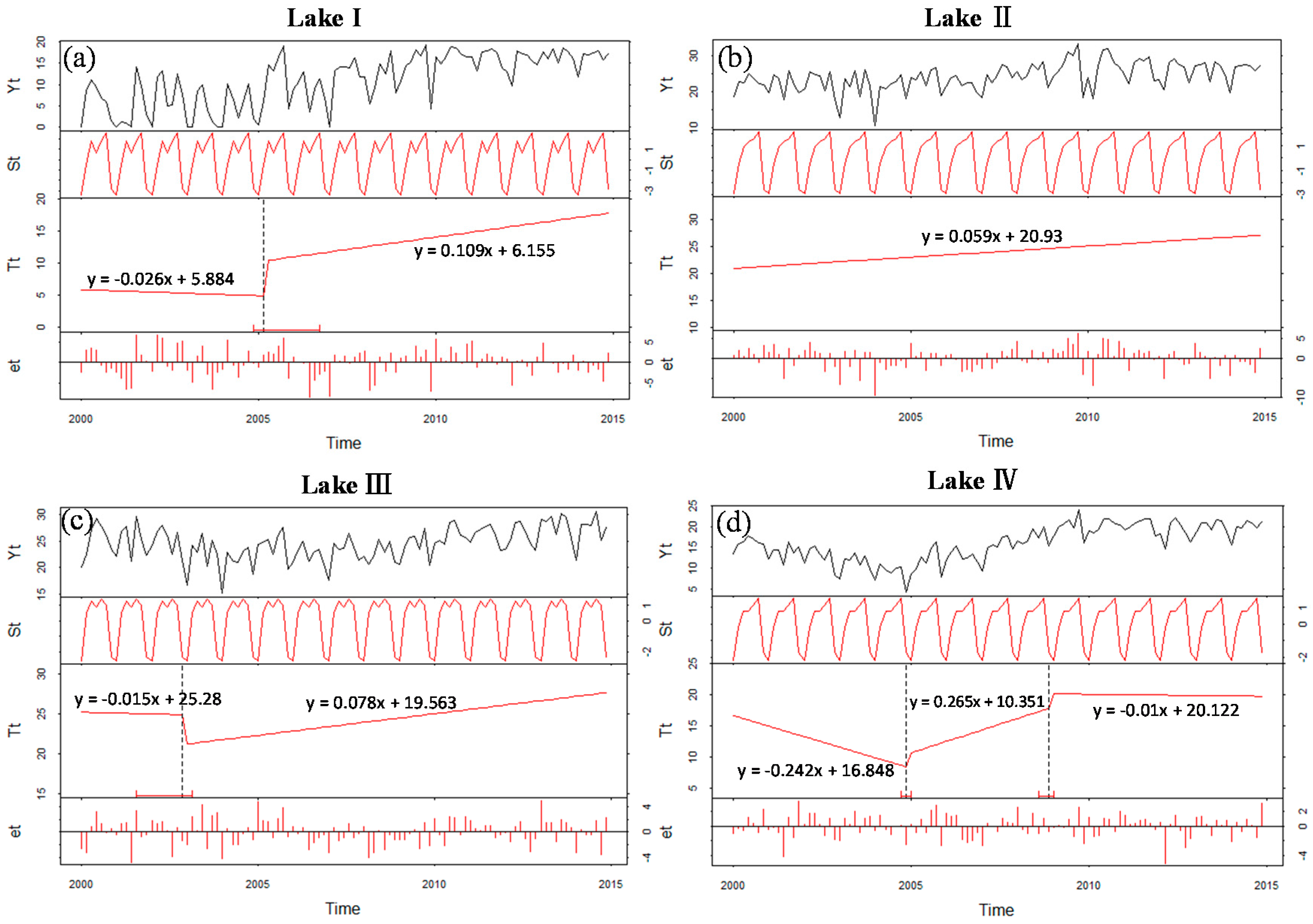
indicates the location of the breakpoints; (a) is the area dynamics for Lake I; (b) is for Lake II; (c) is for Lake III; (d) is for Lake IV.
Remotesensing 09 00082 g008
Figure 9. Fitted seasonal (St), trend (Tt) and remainder (et) components for: monthly temperature (a); and precipitation (b) from 2000 to 2014 (Yt).
Remotesensing 09 00082 g009
Table 1. Part of bands information of MODIS.
BandBand IDResolution (m)Bandwidth (nm)
R1 (B1)250620–670
NIR2 (B2)250841–876
B3 (B3)500459–479
G4 (B4)500545–565
SWIR16 (B6)5001628–1652
SWIR27 (B7)5002105–2155
Table 2. Evaluation (in terms of R2 and RMSD) of the ability to preserve the spectral properties of the observed coarse image.
IndexIMARMARWavelet
MetricsR2RMSDR2RMSDR2RMSD
Band 3 (Blue)0.93.2250.8384.5080.9143.519
Band 4 (Green)0.8993.2270.834.6730.9163.408
Band 6 (SWIR1)0.922.0980.9072.3010.8874.46
Band 7 (SWIR2)0.9571.790.6464.7370.916.339
overall0.9192.5850.8054.0550.9084.4315
Table 3. The error statistics from 500 m observation, original and improved data.
LakesTypeOCA (%)Ec (%)Eo (%)Lake Area (km2)Reference Area (km2)
I500 m86.1619.7613.8314.38213.577
MAR88.541711.4614.328
IMAR90.1213.049.8814.006
Wavelet88.5413.0411.4613.79
II500 m84.117.0215.2923.82725.973
MAR92.157.647.8525.92
IMAR94.424.545.5725.705
Wavelet90.914.559.0924.793
III500 m90.0911.539.9130.26729.783
MAR93.519.916.4930.804
IMAR94.954.865.0429.73
Wavelet93.155.596.8529.408
IV500 m78.237.577.2117.60217.495
MAR88.658.2811.3416.26
IMAR91.726.096.0917.495
Wavelet87.423.6812.5815.938
Table 4. Correlation analysis for four lakes between lakes area and meteorological variables (average monthly temperature (AMT) and precipitation (AMP)).
LakesLake ILake IILake IIILake IV
VariablesAMTAMPAMTAMPAMTAMPAMTAMP
Trend0.9550.9550.9990.9990.6040.6040.7670.767
Season0.4250.4470.4570.4710.6050.6360.4280.452
Fitted_overall0.690.7010.7280.7350.6050.620.5980.61
Unfitted_overall0.1590.2510.2340.2480.2950.2650.1660.194

