A Combined Approach for Filtering Ice Surface Velocity Fields Derived from Remote Sensing Methods


1
Alfred Wegener Institute, Helmholtz Centre for Polar and Marine Research, 27570 Bremerhaven, Germany
2
University of Bremen, 28359 Bremen, Germany
*
Author to whom correspondence should be addressed.
Remote Sens. 2017, 9(10), 1062; https://0-doi-org.brum.beds.ac.uk/10.3390/rs9101062
Submission received: 21 July 2017
/
Revised: 14 September 2017
/
Accepted: 22 September 2017
/
Published: 18 October 2017
Abstract
:Various glaciological topics require observations of horizontal velocities over vast areas, e.g., detecting acceleration of glaciers, as well as for estimating basal parameters of ice sheets using inverse modelling approaches. The quality of the velocity is of high importance; hence, methods to remove noisy points in remote sensing derived data are required. We present a three-step filtering process and assess its performance for velocity fields in Greenland and Antarctica. The filtering uses the detection of smooth segments, removal of outliers using the median and constraints on the variability of the flow direction over short distances. The applied filter preserves the structures in the velocity fields well (e.g., shear margins) and removes noisy data points successfully, while keeping 72–96% of the data. In slow flowing regions, which are particularly challenging, the standard deviation is reduced by up to 96%, an improvement that affects vast areas of the ice sheets.

1. Introduction
The dynamics and mass balance of glaciers governs the contribution of ice sheets to sea level change. Consequently, monitoring changes in the dynamics in high spatial resolution and with a large spatial coverage, like entire ice sheets, is crucial. Also, the temporal evolution of the flow dynamics is very important. This can only be achieved using satellite remote sensing data. The key physical quantity here is the three dimensional velocity field of the glacier , of which, however, only the horizontal velocity at the surface of the ice sheet is accessible. Numerous studies (e.g., [1]) use different sensors and algorithms to retrieve velocity fields, but common to all are measurement errors that lead to noisy velocity fields. False velocity data needs to be filtered out in order to avoid complications in all the following fields of applications.
Timing and spatial onset of changes in velocities, caused by seasonal or longterm climate forcing, is of particular interest to glaciologists. With more accurate velocity fields our ability to detect acceleration is improved. The most prominent example is the acceleration and increased seasonality of Jakobshavn Isbræ in western Greenland. This might be connected to changes in the shear margins of the ice stream, highlighting the need of accurate velocity retrievals in these areas. Here, the gradients of the velocity field components are required with high accuracy, so that shear deformation rates can be retrieved in order to assess if changes in the shear margins are indeed the cause of acceleration.
Numerical models of ice sheets and glaciers use horizontal surface velocities to assess the model quality and partly to adjust model parameters. Simulations projecting the future contribution of ice sheets to sea level change suffer from a poorly constraint initial state, which is today’s velocity field. In order to overcome this, glaciologists use inverse modelling of ice sheets and ice streams, in which basal parameters are adjusted so that modelled horizontal surface velocities match the observed field. As the momentum balance equation, which is solved in inverse modelling, contains gradients of the velocity components (strain rates), the influence of non-smooth velocity data is enhanced. In this case, errors in the input field lead to errors in computed basal parameters and this in turn leads to incorrect projections.
With missions such as Radarsat-1, Radarsat-2, TerraSAR-X, TanDEM-X, Sentinel-1A/B, Sentinel-2 and Landsat-8 a new era of mapping large-scale surface velocities has begun [1,2,3,4,5]. Today surface velocities of ice sheets, glaciers and ice caps are produced in near real-time and several data portals exist where the user can download velocity products. However, as most of these velocity estimates are based on offset tracking procedures, outliers and data gaps are most common and appropriate filtering is absolutely essential before further analysis.
Many of the applications of velocity fields will use an interpolation to obtain continuous velocity datasets which might be used for inverse modelling of glaciers subsequently. Depending on the type of interpolation applied, outliers might have strong effects, as interpolation techniques that rely on higher order polynomials are generally very oscillatory and may produce high amplitude outliers between the interpolation points.
The nature of erroneous data points is twofold. On the one hand, a pixel may have a false value in one or both velocity components. On the other hand, such a false velocity estimate can lead to a false flow direction. Outliers can occur in many different ways, such as covering only one pixel or a cluster of connected pixels. These clusters can be either smooth within themselves, or also very noisy. Other features are appearing over larger areas, like single lines or regular patterns. False velocity retrieval from Synthetic Aperture Radar (SAR) data is caused by different factors: (i) low correlation, caused by changes in the surface properties between data acquisitions (e.g., surface melt or precipitation), (ii) very fast flow is causing poor coherence or (iii) atmospheric and ionospheric effects. Errors induced by atmospheric variations between the dates of data acquisitions can mostly be neglected for velocity retrievals from intensity offset tracking, but can be an issue for velocity estimates from SAR interferometry [6]. Ionospheric effects can result in azimuth streaks in the derived velocity fields [7,8].
Critical zones can be especially slow or fast flowing regions, shear margins or pinning points of ice shelves. Future and current satellite missions in L-band, like ALOS PALSAR-2, NISAR and Tandem-L are preferable for ice velocity retrieval as deeper penetration is beneficial in areas with loss of coherence due to changes in surface properties or very fast flow. However, L-band signals suffer from ionospheric effects leading to errors in velocity retrieval [7,8]. Again, a filter procedure might be able to reduce ionospheric effects in the velocity fields.
This reveals the importance of an appropriate filtering procedure. To avoid manual filtering of outliers, because this would be very time consuming and leads to different solutions for different users, it is possible to use a wide range of algorithms developed for this purpose. A filter needs to fulfill the following criteria: (i) remove erroneous data reliably, (ii) the structure of the velocity field remains unchanged, e.g., shear margins or sticky spots are not smoothed out, (iii) concurrently, as many data points as possible are saved and (iv) reasonable computational costs. Here, we present a filter approach consisting of three different filter steps. This filter will be in future implemented into the Tandem-L product generation.
2. Materials and Methods
Description of the Filter
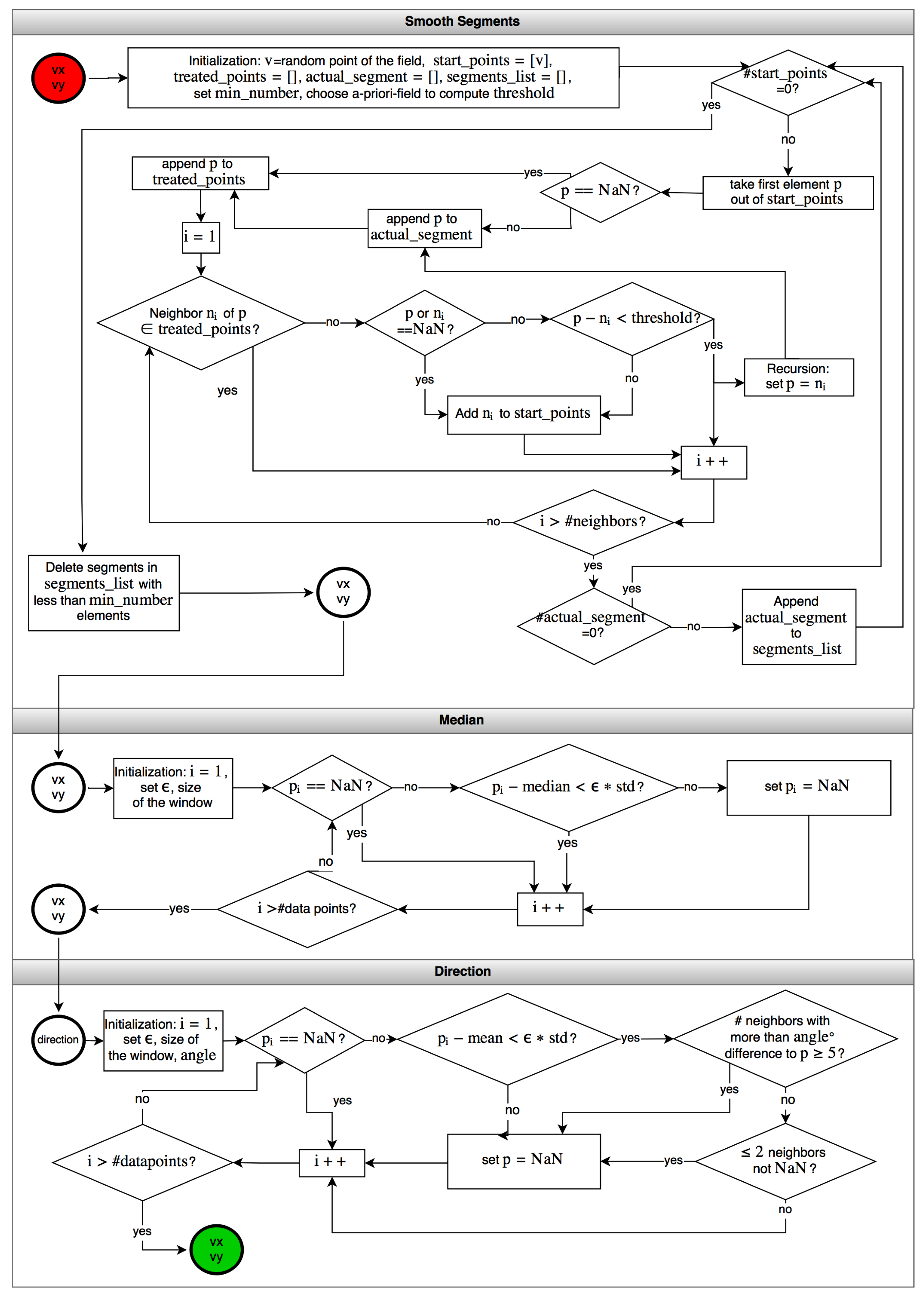
Starting with the projected x- and y-components of the velocity field we applied a filter combining three approaches. The first one divides the field into parts recursively, which are smooth within themselves, and was introduced by Rosenau et al. [9]. In the second step, the remaining outliers are removed by a filter using the median of the field. The third filter is based on variations of directions of the vector field.
In the first component of the filter, all data points in the field are allocated to different segments. Afterwards, segments with less than data points are deleted. The division in segments of the data points is done recursively, starting with a random seed point p. For each direct neighbour n, the difference between the velocity of p and n in both components (x and y) has to be compared with the threshold . Only if it is less than in both velocity components, the neighbor n is allocated to the same segment as p and the procedure starts again with this new point. There are two terms influencing the threshold : These are a constant error and the difference between the same points in an a-priori velocity field multiplied with a factor w (in our case ).
The constant error includes the errors of offset tracking and coregistration and is multiplied by a factor in order to reduce the accepted error, often leading to better results with more points sorted out. In the applications below, we set . We computed these errors like in Seehaus et al. [10], where is calculated from stable points on rock surfaces. For this purpose we figured out coordinates of rocks in the area of the velocity field and computed the magnitudes of the velocities in these locations. If there are no stable points in the considered region, this error has to be estimated with the help of a velocity field with similar characteristics. The error of coregistration is calculated as the median of the magnitudes. The offset tracking error is computed as in (3) and strongly depends on the sensor resolution.
with C, uncertainty in image registration and tracking in pixels [], image resolution [], z oversampling factor and time interval between the images [d]. We assumed and , as it is suggested in Seehaus et al. [10].
The second filter step is performed in a window moving one pixel per step. For every data point p, the medians and the standard deviations of the window in both components are computed. The point is only kept, if the difference between the velocity and the median is smaller than times the standard deviation in both components as described in (4) and (5).
with velocity of data point p in x-direction and velocity of p in y-direction, as well as median of all velocities of the window in x-direction and median of all velocities of the window in y-direction. The parameter can be freely chosen, however, was optimal in our applications. The window size in this filter was set to 25 pixels.
The displacement in x- and y-direction defines the direction of flow, , of each data point. The third approach works with this information, again by using a moving window, which is in our application of the same size as before (25 pixels), but can be chosen independently from the second filter step. With each step, the window is shifted by one pixel. First we check if the direction of a data point p is close to the mean direction of the window (6)
with s standard deviation of all directions in the window and unrestricted parameter proposed to be . Subsequently, the number of direct neighbors n of the point p with having a difference of more than degrees to is counted.
For the angle a value of is proposed. If this number of neighbors is higher than 4, the point is discarded.
In the last step, all points having less than 2 neighbors n with , are removed, because in this case a comparison with neighboring points is not possible. In all three steps, a point which is detected as an outlier in only one component is removed in the other component of the velocity vector. More details to the filter processes can be found in the flowchart in Figure A1. The effect of the choice of the parameters on the performance of the filter is discussed below in more detail.
3. Results
3.1. Artificial Flow Field
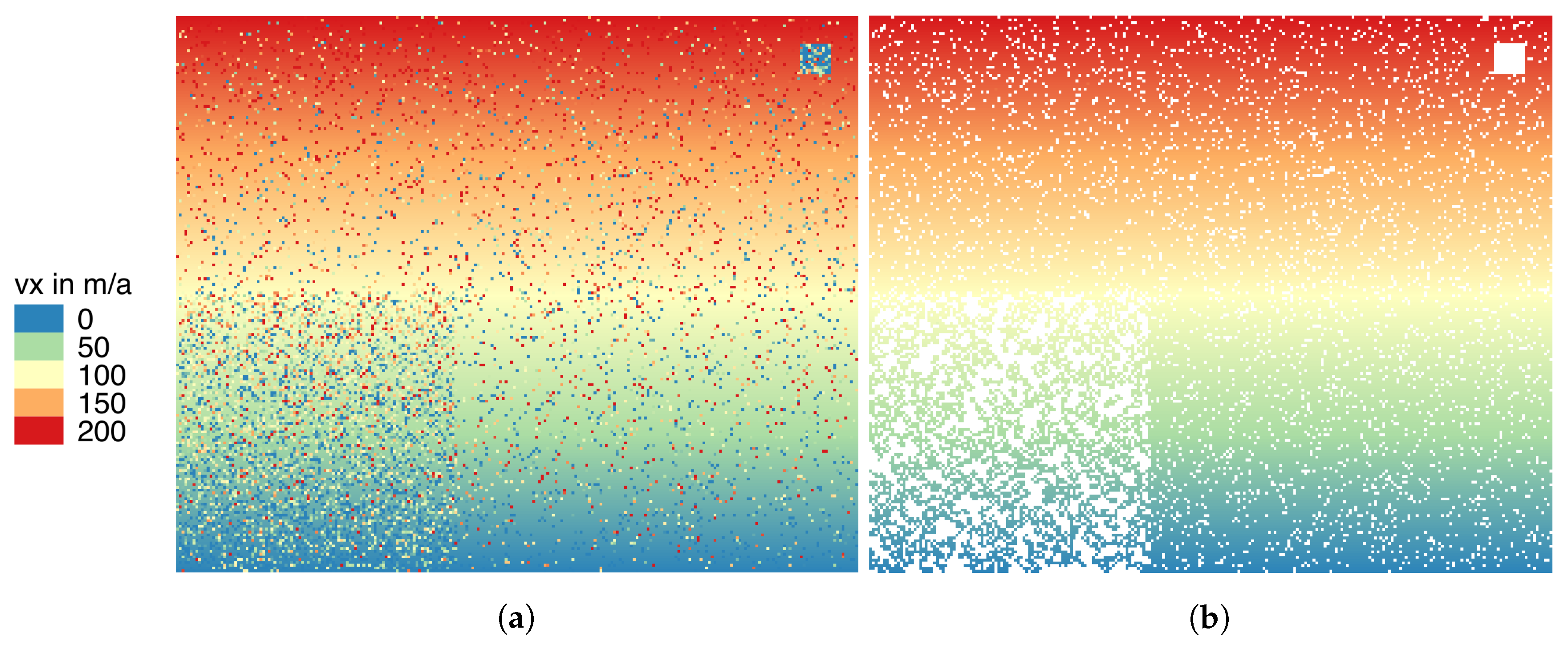
In order to test the performance of the filter, we created an artificial velocity field across which we have distributed outliers randomly. The field has a size of 200 × 245 data points. The a-priori field has increasing velocity values between 1 and 200 m a in x-direction, while the component increases in y-direction from 1 to 245 m a, which leads to different flow directions. We distributed outliers by adding normal distributed values () to 4900 random points of the field. Additionally, we added 5000 values distributed with in a smaller region to simulate strong outliers in a limited area. In the end, in a region with a size of 10 × 10 pixels the velocity values are generated randomly () (Figure 1a). The applied filtering procedure can remove nearly all of these outliers (Figure 1b). Only 0.33% of the generated outliers are left. These outliers have a relatively small difference (maximal 6.07 m a) to the expected values given by the a-priori field. Valid points falsely removed by the filter had less than 2 neighboring points for comparison in the last filter step.
3.2. Filter Parameter Sensitivity Tests
The three filter steps obey a number of parameters. Here we test the influence of these parameters on the ability to filter outliers. As glacier and ice sheet velocity fields contain certain characteristics with distinct challenges for the filter, we selected a subset of a velocity field covering a stripe-shaped area over a fast flowing glacier, including its shear margins and extending into slow flowing areas (the location of the profile is shown in Figure 3d). This subset contains 80,676 pixels of the velocity field, which we consider to be sufficiently large for these tests. For filter step one (smooth segments), we have varied a from to 1 in steps of , from 2 to 12 with increments of 2 and the difference to the a-priori velocity field from 1 to 2 in increments of . For filter step two (median) we tested the effect of the window size () and . was varied from 5 to 45 in steps of 5 and was increased from to in increments of . The third filter step (directions) is influenced by the choice of the window size too, (, varied from 5 to 45 in steps of 5), (from to in increments of ) and the angle (from to with step size ). Figure 2 shows an example of parameter while the remaining parameters can be found in Figure A2 to Figure A6 in the Appendix A.2.
Filter one is highly insensitive to , the range from 4–12 give similar results, only shows a difference. Thus the choice of is reasonable and does not affect the performance of the filter negatively. The effect of a is, however, larger but declines for . With increasing w, the number of points remaining is increasing, which is to be expected, as a higher w is increasing the threshold . Similar to that, is reducing the remaining data points significantly in both, fast and slow flowing regions. The optimal parameter set is thus , and .
The second filter is not particular sensitive to the window size. In the range of 20 to 35 pixel no variation occurs at all and below and above this range, only slight changes in faster flowing areas appear. was thus chosen to be 25 pixels. This filter is more sensitive to the choice of . Low values of remove a large number of data points, while does lead to similar results. An outlier at a distance along track of 57 km exemplifies, that our choice of is suited well to remove this outlier (Figure A5).
The directional filter shows a similar response to the window size, meaning that it is not particular sensitive on the size. The effect of is also similar to the second filter, as small values for remove an unreasonable high number of data points and the range does lead to similar results. The effect of is strongest in slow flowing areas, in which we also expect the largest number of false directions. From the number of remaining data points increases in a way that the filter becomes meaningless. At the other end of the spectrum of values for , the number of remaining data points becomes critical for . Hence our choice is , the window size is set to 25 pixels and . These values may serve for other applications of the filter as a first guess, however, we recommend users perform similar tests for their particular areas and sensors for optimising the performance.
3.3. Recovery Glacier
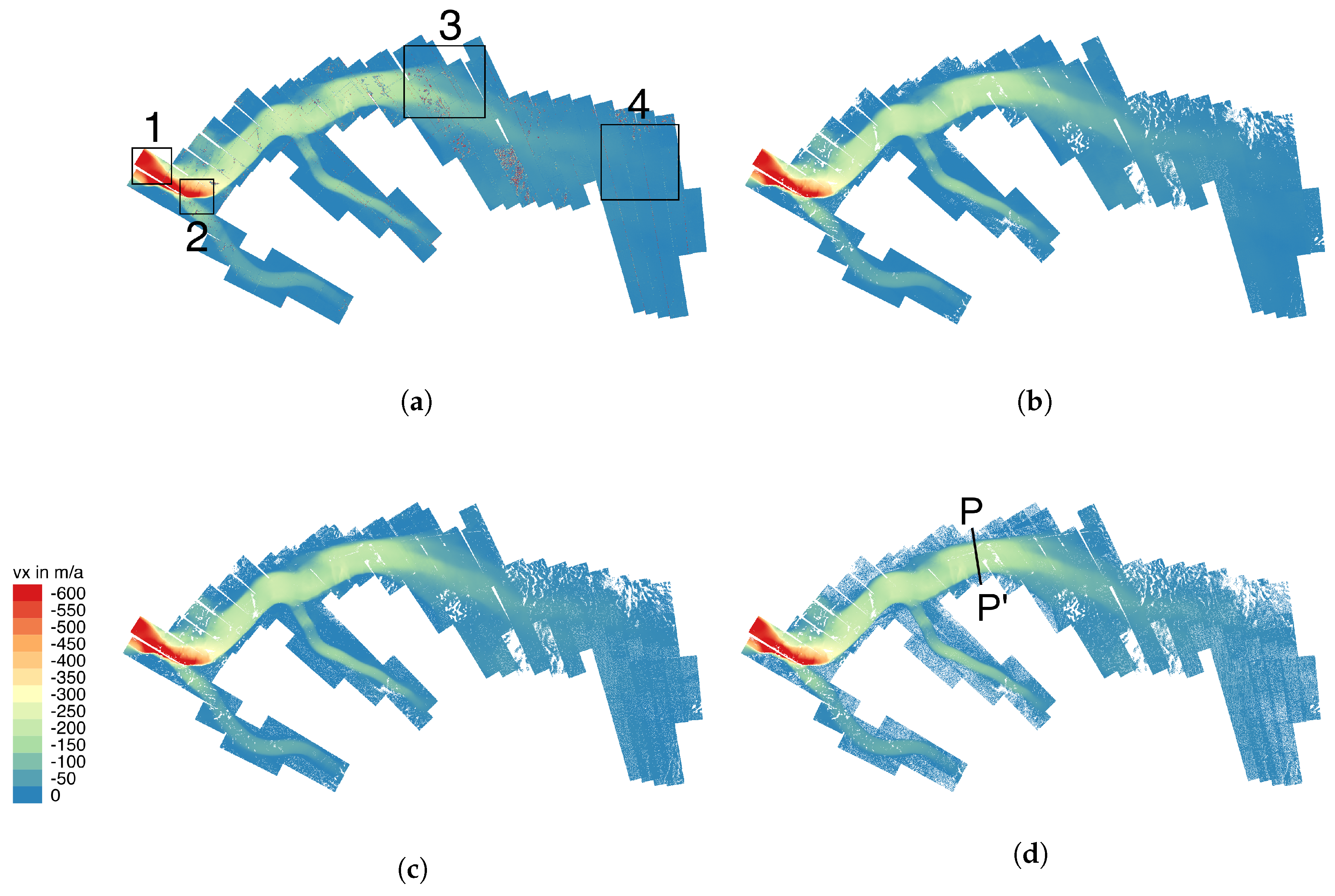
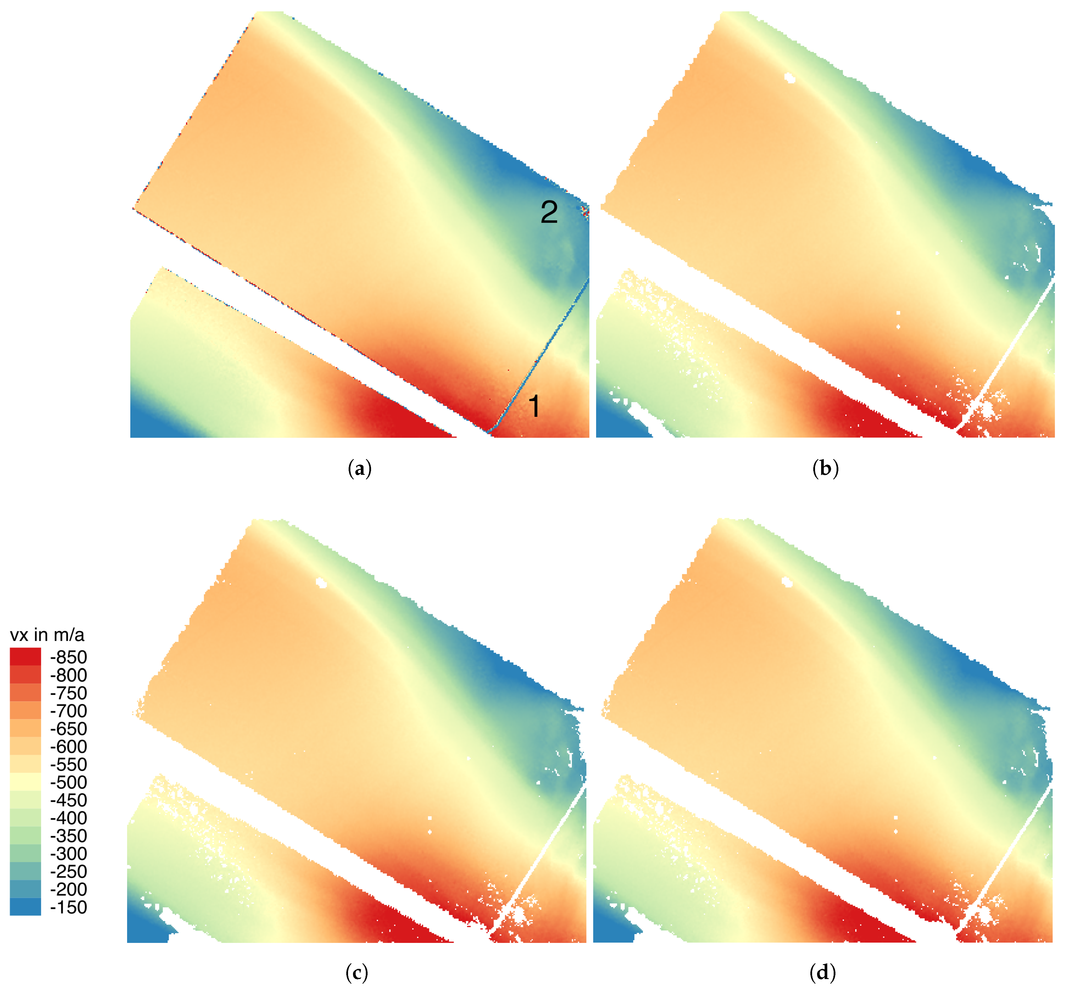
We applied the filter to a velocity field of the Recovery Glacier (Antarctica, Figure 3a). The data are derived by intensity offset tracking of stripmap pairs of TerraSAR-X in 2012/13 and were provided by DLR in Floricioiu et al. [11] and Abdel Jaber [12]. The revisit time was eleven to 33 days and the resolution of the velocity field is 156 m. Every individual velocity field retrieved from one pair of satellite scenes was filtered separately to preserve as much data points as possible. Thus, overlapping scenes can compensate for removed outliers. As an a-priori velocity field for the smooth segments filter we used the Making Earth System Data Records for Use in Research Environments (MEaSUREs) ice velocity map of Antarctica [13,14]. Afterwards the field was mosaicked by gmt grdblend [15] using the mean of overlapping pixels. We have done this also for the fields after the first two filter steps to illustrate the results. Figure 3 shows the original field and the results after each filter step. This figure demonstrates that the first filter (upper right panel) removes most outliers that are visually detectable on this scale. The next two steps (panels below) remove still a markable number of outliers, however keeping a reasonable amount of data. As the scale of the figure does not allow any detailed discussion of the effects, we selected four different sites for an in-depth discussion, with very distinct characteristics: one fast and one slow moving region, a shear margin and a region with a very high number of outliers (named line of outliers in the continuation). These regions are annotated in Figure 3a.
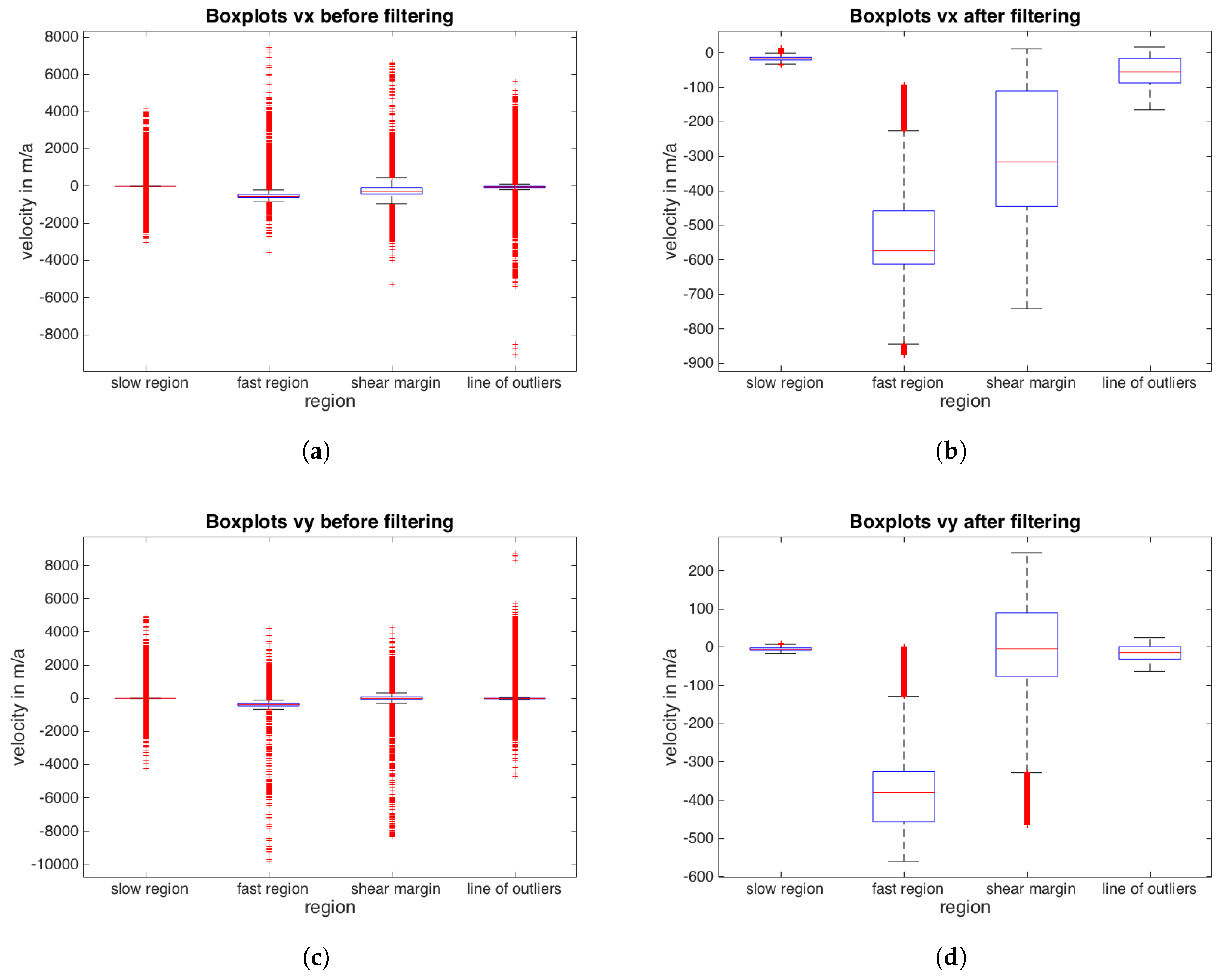
In order to give some quantitative information on the statistics of the effect of the combined filter, we present boxplots for all four regions in Figure 4 for both components, and . The left panels show the original data, whereas the right panels present the statistics after the application of all three filter steps. Please note that the vertical axis changes between the left and right panels. In all cases the number of outliers is significantly reduced and the range of values is diminished. The range of the quartiles in and becomes smaller. The efficiency of the filter to remove outliers is also evident from Table 1. For three of the four subregions, as well as for the whole mosaic, the standard deviation decreased significantly during the filtering while the mean stays rather constant. For example: while the mean from the line of outliers changed by 3.4%, the standard deviation was reduced by 76.6% during the filtering (Table 1). This difference is less striking in regions with more heterogeneous flow velocities, for example in the shear margin. In this example the mean changed by 9.1% while the standard deviation was reduced by 27.3%. In order to investigate the effect of the three filter steps in-depth, we discuss below the field for the four regions after each filter step.
3.3.1. Shear Margin
This subset (Figure 5) is a shear margin with a transition from the main trunk of the glacier to nearly stagnant motion and the inflow from a side branch into the main trunk. The first filter step (smooth segments) removes clusters of outliers (marked 1 and 3 in Figure 5a) successfully and also eliminates the outliers along the margins of the satellite scenes (denoted with 2). The second filter (median) removes more data points with low , which is also the range (marked with 4 in Figure 5d) with the strongest effect of the third filter (directions). In comparison of Figure 5a and d, the most obvious outliers are captured, however, a stripe-like pattern (denoted with 4 in Figure 5d) is still present after all filter steps. The comparison between the initial and final field of also reveals that the number of data points in the shear margin itself is strongly reduced and patches without data appear, however, there are enough remaining data points to assure that a subsequent interpolation would be able to represent the shear margin well.
3.3.2. Fast Flowing Region
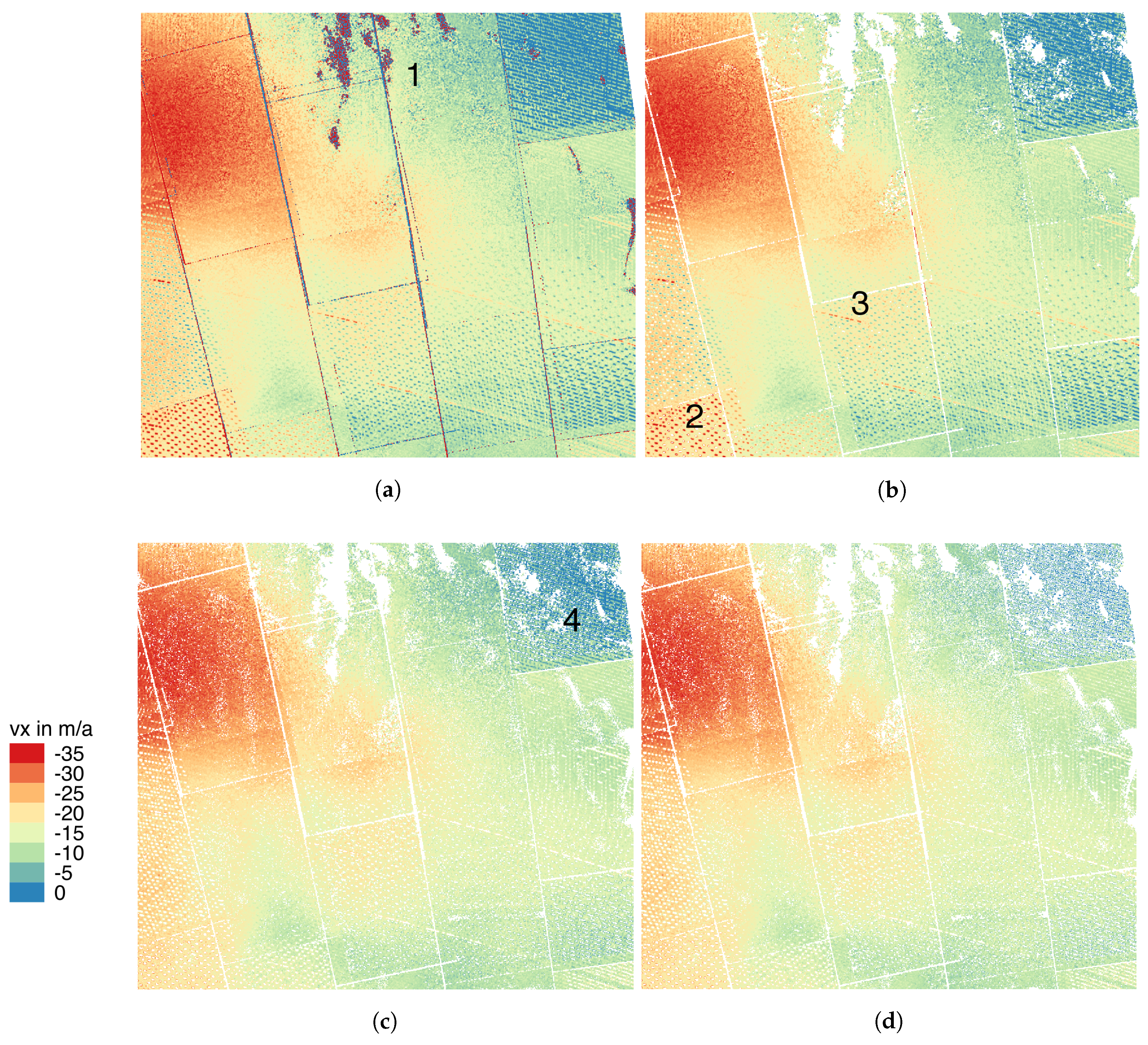
We also chose a very fast flowing region, typical for the central part of ice streams (Figure 6) with displacements up to 800 m a to test the filter. After the first step, the outliers at margins of the satellite scenes are removed. The cluster of outliers around 2 in Figure 6a are also well detected. In the zone labeled with 1 large variations in are removed successfully. Here, the glacier surface is heavily crevassed, which might be the cause for false velocity detection. The median and directional filters do not remove a significant number of data points in this case. This was to be expected, as wrong flow directions are typically a problem in slow moving areas.
3.3.3. Slow Flowing Region
The subset in Figure 7 is characterised by low velocities, which are typically prone to problems in both, magnitude as well as direction of flow. Consequently, a lot of erroneous data points are exhibited in Figure 7a. The first filter removes the clusters, like those marked with 1, successfully, but leaves much more outliers than in the case of the fast flowing region and the shear margin. The second filter is most effective with outliers like the ones marked with 2 and 3. In this example the effect of the directional filter becomes more apparent: the area around 4 has been stripped off a large number of data points. However, there are still invalid data points remaining in this region. As the difference between the data points in this area is small, a subsequent interpolation is not expected to be affected substantially.
3.3.4. Line of Outliers
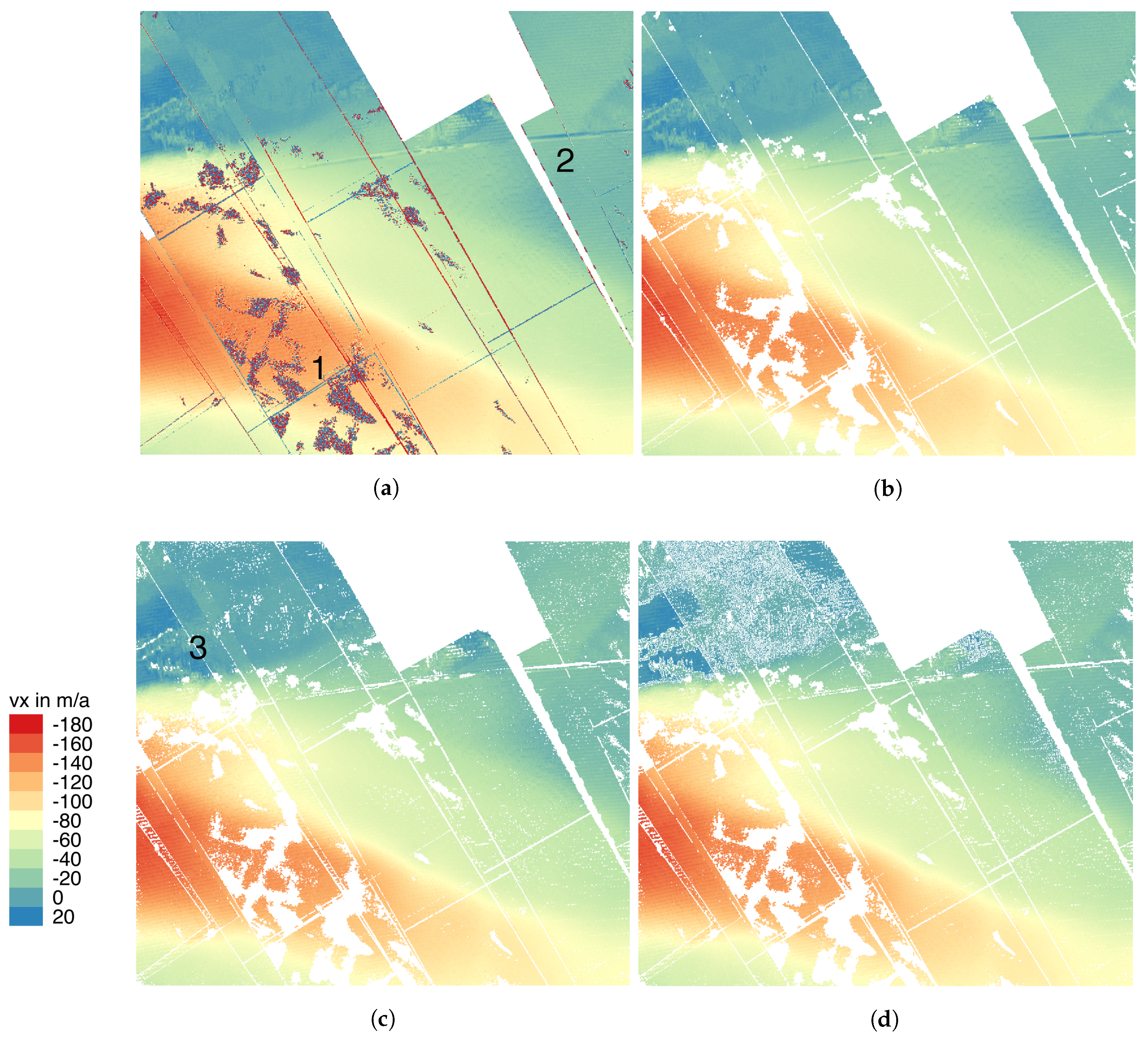
A large number of outliers is evident in the region shown in Figure 8. Beside the clusters of outliers (marked with 1) that also appeared in the other examples, there is a notable feature: a line running through the velocity field of the entire glacier. The first filter step detects these clusters well, as in the examples above. However, the feature 2 is not detected. After the second filter, the line is almost completely erased, whereas the outliers in the region marked with 3 remain. The last filter step has the strongest effect in the area around 3 and the adjacent region of low velocities. This is in agreement with the above examples where the directional filter is most effective in slow moving areas.
3.4. Other Locations
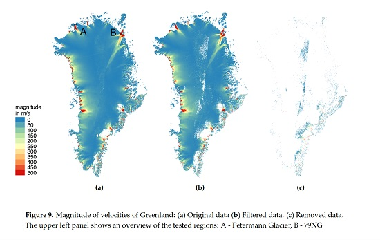
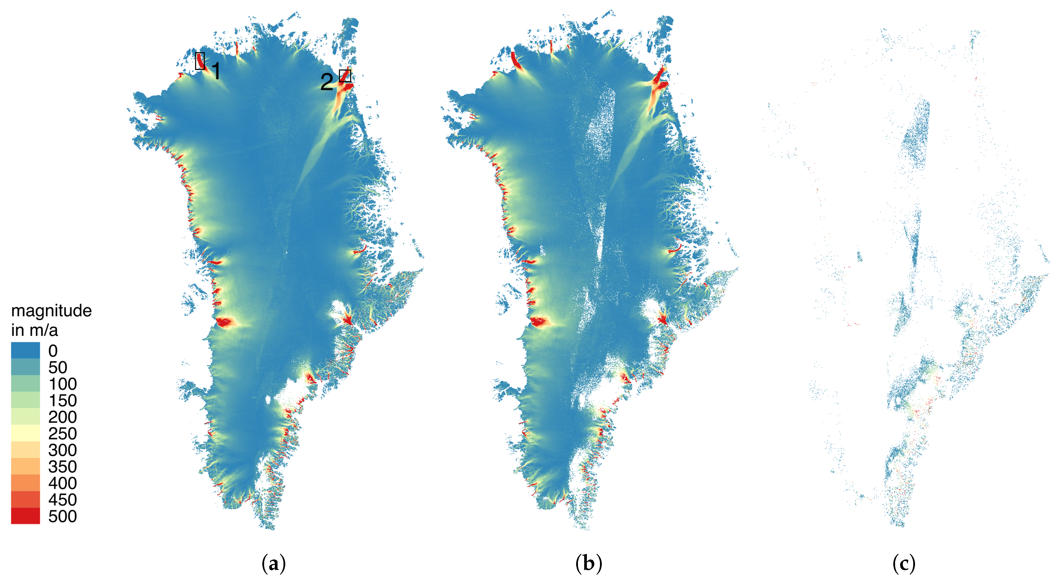
Next to the Recovery Glacier in Antarctica, we tested the filter in some more regions in Greenland. Here we chose a Sentinel-1 velocity mosaic of the Greenland Ice Sheet, a TerraSAR-X derived velocity field of Petermann Glacier and a part of a Sentinel-1A velocity field of a subset of the North East Greenland Ice Stream (NEGIS). These regions are annotated in Figure 9a.
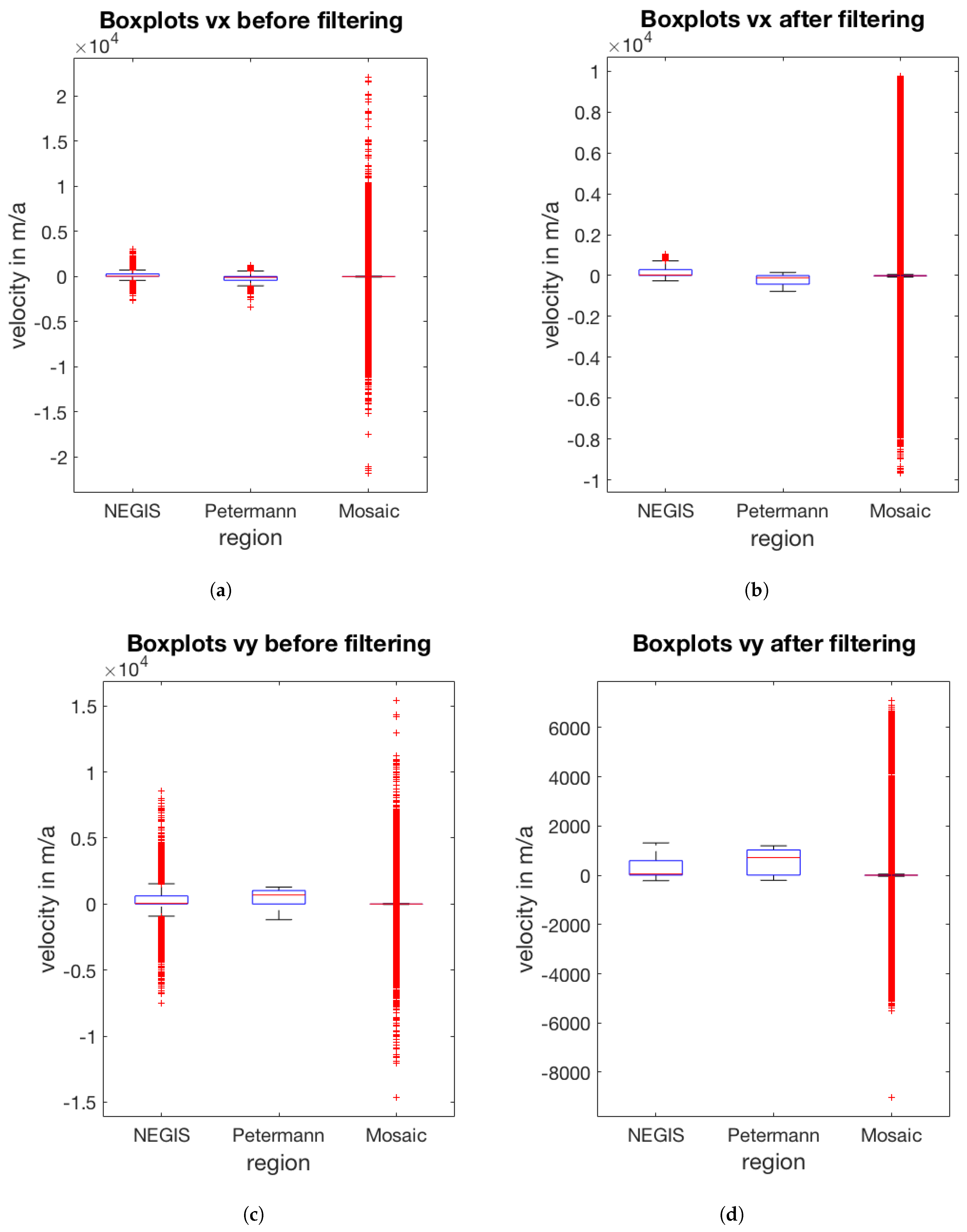
Figure 10 shows boxplots for the three regions, indicating in the upper panels and in the lower ones. The left panels show the original data, while the right panels represent the data after the three step filtering approach. From the boxplots it becomes evident, that the number of outliers could be significantly reduced for the NEGIS subset. This applies for both components and . However, a minor reduction of the standard deviation as evident from Table 1 implies that only few large outliers were present and fast and low velocities coexist in this example. The Sentinel-1 velocity mosaic of Greenland covers a wide range of velocities in both directions wherefore the effect of successfully removed outliers becomes hidden in the boxplots shown in Figure 10. The latter also applies for the minor reduction of the standard deviation in this example as shown in Table 1. The small reduction of 0.4% of the standard deviation of for Petermann Glacier can be attributed to the fact that only few outliers were present in this example (Table 1). In the following, the effects of the presented filtering strategy on the three test regions in Greenland are shown in more detail.
3.4.1. Sentinel-1 Greenland Velocity Mosaic
The velocity mosaic of the Greenland Ice Sheet was obtained by intensity offset tracking on 6-day repeat-pass Sentinel-1A/B acquisitions. For this we employed all available Level-1 Single Look Complex (SLC) products acquired in IW TOPS mode between 1 December 2016 and 1 March 2017 resulting in a total amount of 1779 image pairs. Prior to the coregistration of image pairs, successive bursts of each acquisition were mosaicked. Then intensity offset tracking was performed as described in Appendix A.1. After testing several window sizes we choose a final search window size of 1000 m in both range and azimuth directions. Offsets with a normalized cross correlation below 0.1 were considered erroneous and excluded from the analysis. The single velocity fields were gridded to 250 m and masked by a manually adjusted version of the Bedmachine ice mask [16,17]. This excluded large areas of open water and hence reduces the computation time of the filtering steps significantly. After filtering of the single velocity fields mosaicking was performed as described in Section 3.3. It is very important that the a-priori velocity field used in the first filtering step (smooth segments) has a good spatial coverage. We therefore make use of the MEaSUREs Multi-year Greenland Ice Sheet Velocity Mosaic which shows no data gaps but includes data acquired between 1 December 1995 and 31 October 2015 [18].
While Figure 9a shows the Sentinel-1 velocity mosaic of Greenland prior to the filtering, Figure 9b shows the data after applying the three step filtering approach. The excluded velocity measurements are shown in Figure 9c. It becomes evident, that most removed data points are located in the central part of the ice sheet and in its south-eastern part. On the one hand the acquisition of Sentinel-1A/B data is concentrated on the margins of the Greenland Ice Sheet as these are the dynamical key regions. Therefore, less velocity fields could be derived in the interior of the ice sheet, leading to a decreased ability to fill gaps from multiple data takes. On the other hand low velocities of <20 m a are prevailing in this region. Similar to the slow flowing region of Recovery Glacier, this region is strongly affected by the median and the directional filter. It is also evident from Figure 9, that many data points were removed in the south-eastern part of the ice sheet. This region is known to have poor coherence due to frequent snowfall wherefore velocity retrieval is difficult in this area [1,3]. This large-scale example shows that the applied filtering strategy is capable to discover regions in which the offset intensity tracking poses challenges. Thus it is also conceivable to think of the filter as a tool to investigate systematically the locations in which velocity retrieval is difficult. Individual fast flowing outlet glaciers, where the offset tracking often relies on surface features remain well preserved during the filtering procedure.
3.4.2. Petermann Glacier
For the Petermann Glacier we show a 2014 winter velocity field generated by intensity offset tracking on a 11-day repeat-pass TerraSAR-X/TanDEM-X acquisition following the approach described in Appendix A.1. After testing several window sizes we choose a search window size of 250 m in both range and azimuth directions, which is close to window sizes employed in earlier studies (e.g., [10,19]). Offsets with a normalized cross correlation below 0.1 were considered erroneous and excluded from the analysis. The final velocity field was gridded to 50 m.
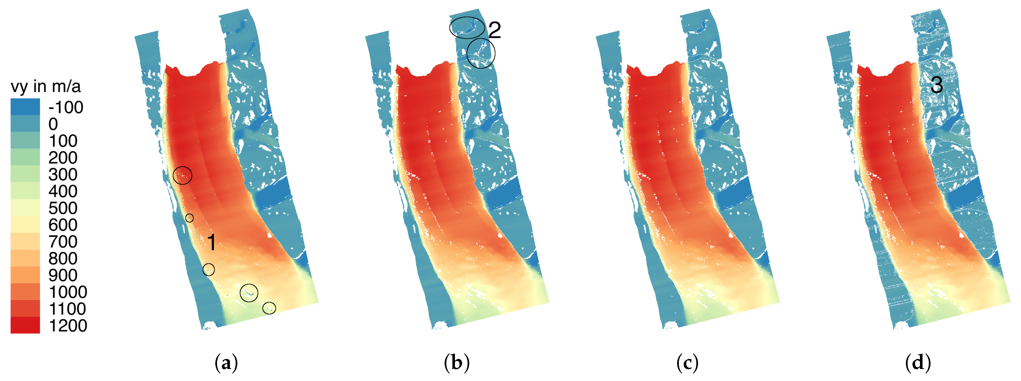
Figure 11 shows the field of Petermann Glacier, which represents the main flow component. Obvious outliers are marked as 1 in Figure 11a and are removed during the first filtering step (smooth segments, Figure 11b). Also several data points of the side margins of two tributary glaciers are removed by the smooth segment filter (marked as 2 in Figure 11b). The median filter leads to more data gaps in both of the mentioned tributary glaciers. The directional filter removes several data points on stable ground (marked as 3 in Figure 11d). As the field of Petermann Glacier is almost in the azimuth direction of the satellite scene, some minor ionospheric effects remain visible.
3.4.3. NEGIS Subset
Compared to the smooth TerraSAR-X velocity field of Petermann Glacier we selected a rather noisy velocity field of a subset of NEGIS to further test the presented three step filtering strategy. The velocity field is based on two Sentinel-1A scenes acquired on 2 March 2016 and 14 March 2016. The data were processed as described in Section 3.4.1 and Appendix A.1.
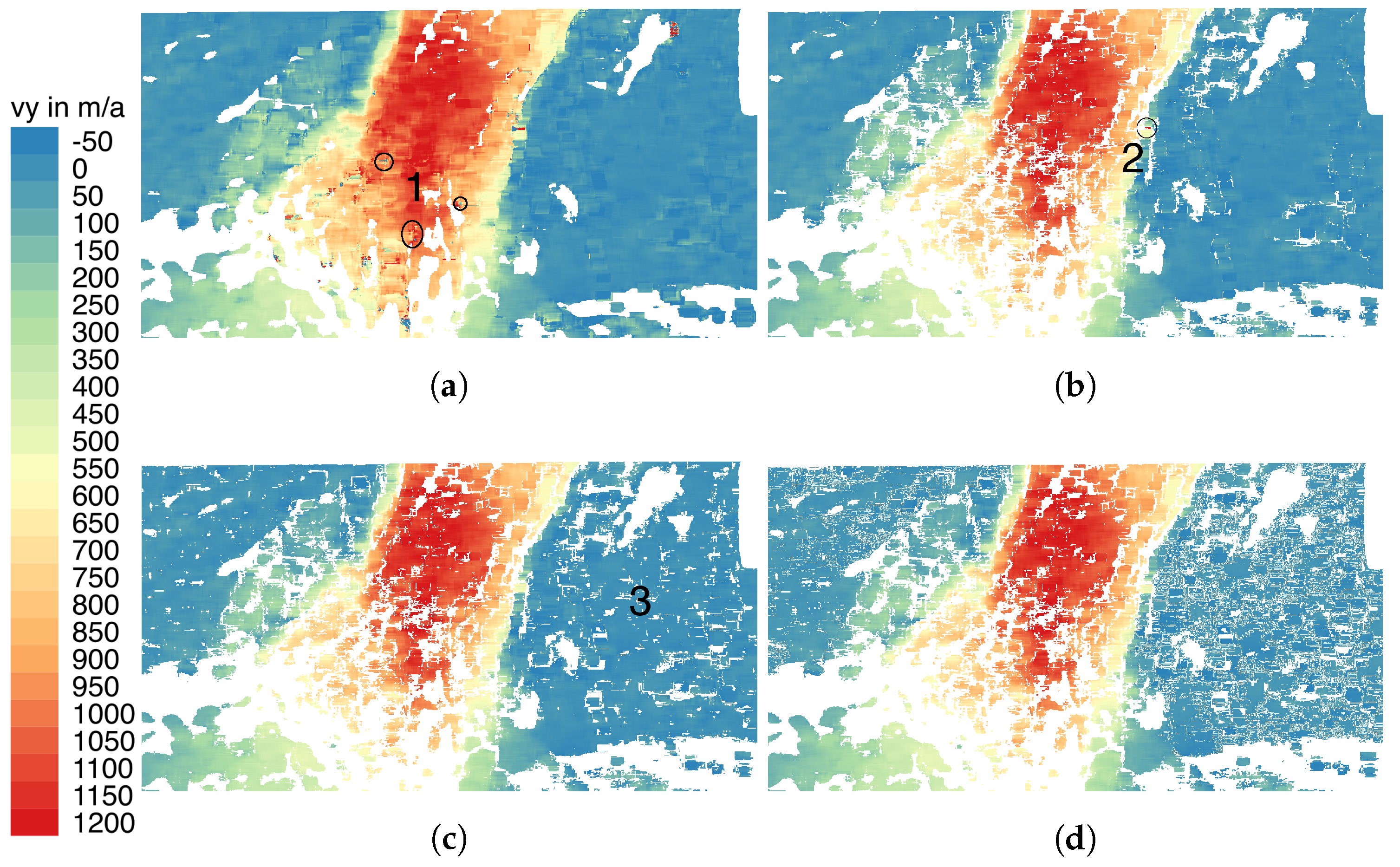
The velocities in y-direction are presented in Figure 12. The original velocity field is shown in Figure 12a, the results of the first filtering step (smooth segments) are presented in Figure 12b, while Figure 12c,d show the data after applying the second (median) and third (directions) filtering step respectively. Contrary to the fast flowing region of Recovery Glacier, outliers are also evident in fast flowing regions of >600 m a (marked as 1 in Figure 12a). Most of these outliers are successfully removed after the first filtering step (smooth segments, Figure 12b). However, some outliers, e.g., in the shear margin (marked as 2 in Figure 12b) are still present. These specific outliers are removed by the second filtering step (median, Figure 12c). Also several data points on stable ground are deleted by the median filter (marked as 3 in Figure 12c), an effect which is further amplified by the third (directions) filtering step. In this example the filter is able to remove many erroneous data points (i.e., only 71.58% of the original data points are remaining, Table 2). However, depending on the further analysis an additional smoothing and interpolation step might be necessary for this example.
4. Discussion
Our results demonstrate that the presented three step filtering strategy is capable to remove the majority of outliers from remote sensing derived surface velocity fields. Despite a positive qualitative impression when comparing the filtered velocity fields with the unfiltered input fields (e.g., Figure 3, Figure 5 and Figure 7) a quantitative test on a synthetic velocity field with randomly included outliers revealed that the presented filtering strategy removes up to 99.67% of erroneous data points (Figure 1). On the other hand a maximum of valid velocity measurements is preserved throughout the filtering. While from the rather noisy velocity field of the NEGIS subset 28.42% of data points were removed by the filter, up to 95.60% of valid velocity measurements were preserved for the relatively smooth velocity field in the fast flowing region of Recovery Glacier (Table 2).
The three step filtering strategy applied in this study relies on several parameters which can be adjusted by the operator. In the first filter (smooth segments) these include a, w, and . Lower values of in (2) would lead to a lower threshold during the classification of segments. As a result, segments would have less elements and consequently more points would be removed. A higher value can be chosen if the filtering procedure should be more defensive. Our sensitivity analysis showed that a value between 0.2 and 0.4 removes most erroneous data points (Figure A3). The factor w is designated to account for possible temporal changes between the a-priori velocity field and the satellite derived velocity field [9]. It is therefore highly dependent on the expected changes in the study region. Here we propose a value of 1.5 for regions where we expect little changes between the a-priori velocity field and the raw input velocities. The number of elements in a segment to be accepted, , is already proposed in [9]. We can confirm this in Section 3.2, however, the result for between four and twelve seem to be very similar. A higher value of can improve the result, if there are larger outlier areas, which are very smooth within themselves. The offset tracking error in (3) is dependent on the resolution and the revisiting time of the employed satellite and need to be adjusted correspondingly by the operator (e.g., [10,20]).
In the second filter (median) the parameter and the size of the moving window can be changed. in (4) and (5) influences the threshold below which data points are deleted and therefore the amount of removed points directly. The window size should be larger than the size of the erroneous features, as otherwise the filter is not able to remove them. At the same time, the window size should depend on the resolution of the velocity field. A larger window leads to the removal of more points, causing problems especially in shear margin regions. Therefore, this parameter should be reconsidered in case of loosing too much data points during the second filtering step. However, the size of the moving window plays also an important role for the computation time. If a reduction of the computation time is necessary, e.g., in the case of high resolution input data or large spatial coverage, a reduction of the window size should be considered.
In the third filter (directions), the angular threshold in (7) and the size of the moving window can be adjusted by the operator. A changing value of has the strongest effect in slow flowing areas as there are only little differences between two satellite images with a small time interval in between. Therefore, the direction of the flow cannot be detected in many cases. This problem does not appear in fast flowing areas, wherefore the strongest effect of the directional filter is evident in slow moving regions.
Previous remote sensing studies rely only on one of the presented filtering steps to exclude outliers from satellite derived velocity fields. While most large-scale studies of ice streams and ice sheets rely on filters based on local variance within a moving search window (e.g., [3,21]), studies examining mountain glaciers also make use of directional filters employing certain angular thresholds to which neighboring data points are allowed to deviate (e.g., [22,23]). In order to find segments of continuous glacier flow Rosenau et al. [9] implemented a gradient based filtering approach. The latter has been successfully applied on Landsat derived velocity fields for numerous outlet glaciers in Greenland [9].
In this study, all of these approaches were connected in series. This way erroneous data points are successfully removed even if an outlier is not detected in the previous filtering step. This is evident for example in the shear margin of Recovery Glacier (Figure 5). In this example, 54.23% of the removed data points were detected by the first filter (smooth segments), 12.04% by the second filter (median) and 33.73% by the third filter (directions).
Our results show that the different methods used in the three filtering steps have different effects on the velocity field. While the first two steps remove clusters which are noisy in magnitude, the last one removes data points with false flow directions. The segment filter can remove clusters, which are smooth within themselves but having an offset to surrounding points. The median filter on the other hand is capable to remove features with a smoother transition from correct to incorrect data points. We found, that the order of the three filtering steps has a significant impact on the results. We therefore tested all possible arrangements and the presented procedure turned out as being most effective. The major cause for this is, that the first filter relies on segments, meaning that once the second and third filter steps were removing individual points, there were less clusters and with that the first filter becomes less successful.
In this study, it has been shown that the combination of three separate filtering algorithms is very effective for removing outliers from surface velocity fields. However, it should be noted that it is not possible to employ the complete filtering strategy for all settings of glaciers. This is mainly because an input to the segmentation filter is an a-priori velocity field with a good spatial coverage. In this filtering step, the difference of neighboring points in the a-priori field is taken to compute the accepted error between two points in a segment. This means, that a missing value in the a-priori field would also lead to a missing value in the result, even if the corresponding value is a valid velocity measurement. For the examples shown in this study, this is not a problem as we rely on large scale high resolution ice motion fields available through the MEaSUREs program. These mosaics were compiled from data of various remote sensing sources including ALOS PALSAR, Envisat ASAR, ERS-1/2, Landsat-8, RADARSAT-1/2 and TerraSAR-X and show no gaps in our study regions. For many mountain ranges no such compilations are available yet, specifically for smaller mountain glaciers. This limits the use of the smooth segment filter in these regions. However, it has been shown previously, that filters based on local variance within a moving search window or a directional threshold are capable to remove many outliers in such areas [22,23,24,25]. We therefore argue, that even if the smooth segment filter fails in these areas, robust results might be obtained by employing the median filter and the directional filter.
5. Conclusions
We presented a new approach to filter outliers of remote sensing based glacier velocity fields. The approach consists of three individual steps, with each filter detecting different types of incorrect data points. The combination of the three filter steps leads to a robust filtering of data, so that the standard deviation of the velocity field is reduced significantly, while a reasonable number of data points (72–95%) is preserved. Velocity retrieval is particularly challenging in slow moving areas, which leads to standard deviation values up to a factor of ten of the mean velocity. With our filter, this can be reduced to a factor of 0.5 to 1, leading to datasets with acceptable measurement errors. Also in areas of high velocities, the standard deviation is significantly reduced, leading to higher accuracy in estimates of ice discharge at grounding lines of fast ice streams and hence improved measurement of mass loss of ice sheets. As the procedure does not manipulate the values of the velocity field, no smoothing of velocity gradients occurs, which is important for glaciological applications. Due to its efficiency, this filtering processor is also suitable for future missions dealing with big data volumes.
Acknowledgments
This project is funded by the Helmholtz Alliance Remote Sensing and Earth System Dynamics (HGF-EDA). TerraSAR-X data has been acquired under AO danaf_HYD2059 and ATI_GLAC0267 by DLR. We greatly acknowledge the velocity data provided by Dana Floriciou and Wael Abdel Jaber, DLR. Two anonymous reviewers have helped to improve the manuscript considerably.
Author Contributions
C.L. has implemented the filter, applied it and tested it, N.N. has derived velocity fields of Greenland, Petermann Glacier and NEGIS subset, A.H. has designed the study and supervised it. All authors contributed to the writing and continuously discussed the results.
Conflicts of Interest
The authors declare no conflict of interest. The founding sponsors had no role in the design of the study; in the collection, analyses, or interpretation of data; in the writing of the manuscript, and in the decision to publish the results.
Abbreviations
The following abbreviations are used in this manuscript:
| ALOS PALSAR-2 | Advances Land Observing Satellite Phased Array type L-band Synthetic Aperture Radar Mission |
| NiSAR | NASA-ISRO Synthetic Aperture Radar Mission |
| TOPS | Terrain Observation with Progressive Scans |
| IW | Interferometric Wide |
| SAR | Synthetic Aperture Radar |
| DEM | Digital Elevation Model |
| GNSS | Global Navigation Satellite System |
| DLR | German Aerospace Center |
| NEGIS | North East Greenland Ice Stream |
| SLC | Single Look Complex |
| MEaSUREs | Making Earth System Data Records for Use in Research Environments |
| RG | Recovery Glacier |
Appendix A
Figure A1.
Flowchart of the filter algorithm.

Appendix A.1. Intensity Offset Tracking
In this study surface velocities are obtained by intensity offset tracking on spatially lower resolved Sentinel-1 Terrain Observation with Progressive Scans (TOPS) Interferometric Wide swath (IW) SAR data (∼2.3 m × 13.8 m in range and azimuth) and spatially higher resolved TerraSAR-X stripmap data (∼1.4 m × 1.9 m in range and azimuth). While a full Sentinel-1 scene covers an area of approximately 250 km × 200 km on the ground a TerraSAR-X stripmap scene is restricted to approximately 30 km × 50 km resulting in a trade-off between spatial resolution and ground coverage between both sensors. Independent of the sensor, repeat-pass acquisitions of the respective satellite need to be available for applying intensity offset tracking. While the repeat-pass of Sentinel-1A/B takes 6 days the revisiting time of TerraSAR-X is 11 days. In a first step data from successive repeat-passes of the respective satellite are coregistered based on precise orbit information and a digital elevation model (DEM). A great advantage of this new generation of SAR satellites is that precise orbit information is aided by an on-board Global Navigation Satellite System (GNSS) receiver. Therefore, no stable ground control points or global fits are required for the initial coregistration of repeat-passes and a precise coregistration over moving ice surfaces is possible [3,26]. For each coregistered image pair offsets in range and azimuth direction are then calculated by cross correlating the backscatter intensity in predefined moving search windows (e.g., [27]). In order to improve the accuracy of the estimated shift an oversampling factor is applied to the correlation function [28]. Depending on the spatial resolution of the sensor and the anticipated ice movement between satellite passes the size of the search window is adjusted by the operator. Range and azimuth offsets are finally translated into metric surface displacements and projected into a polar stereographic coordinate system.
Appendix A.2. Filter Parameter Sensitivity Tests
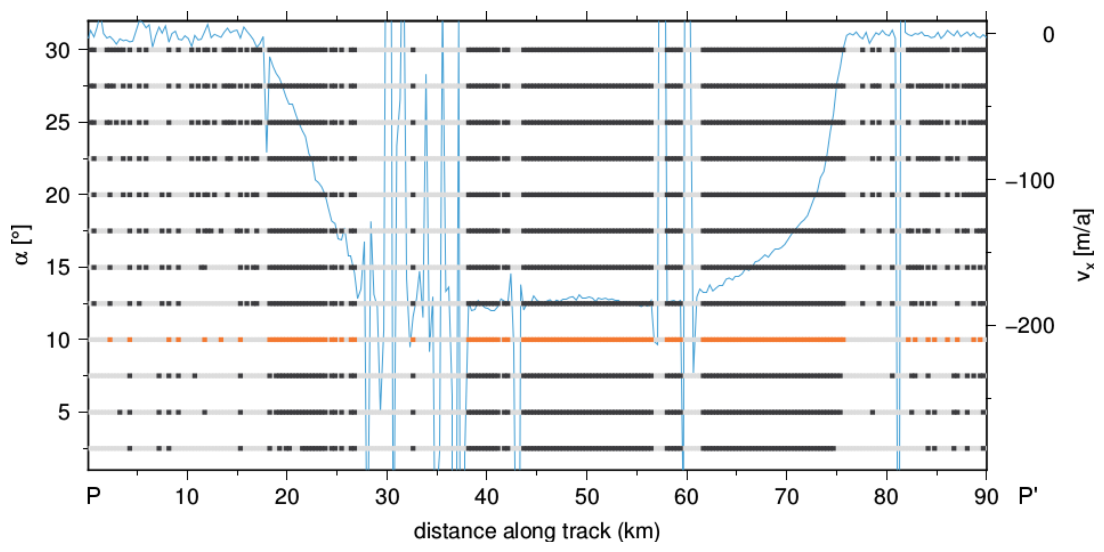
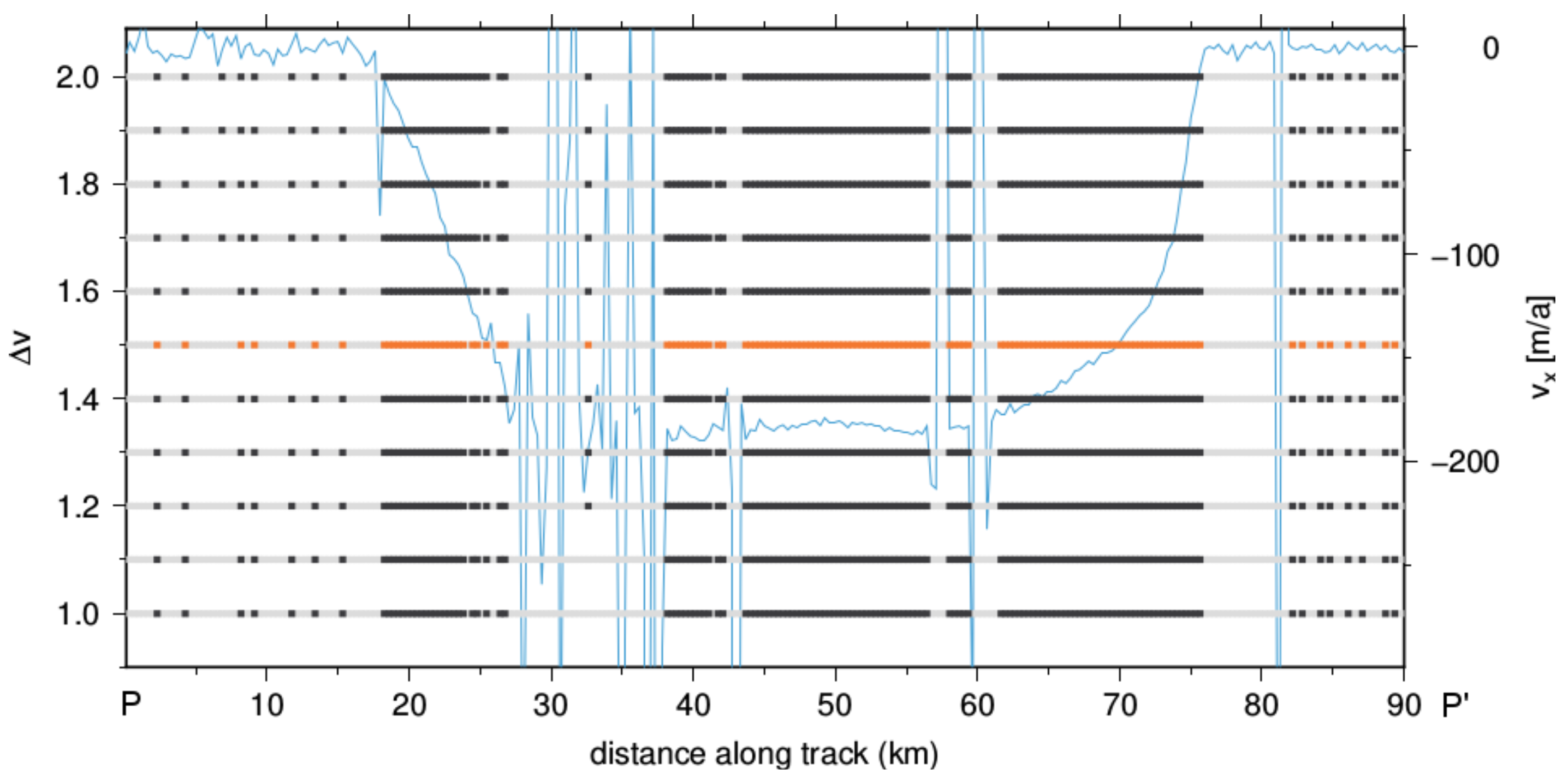
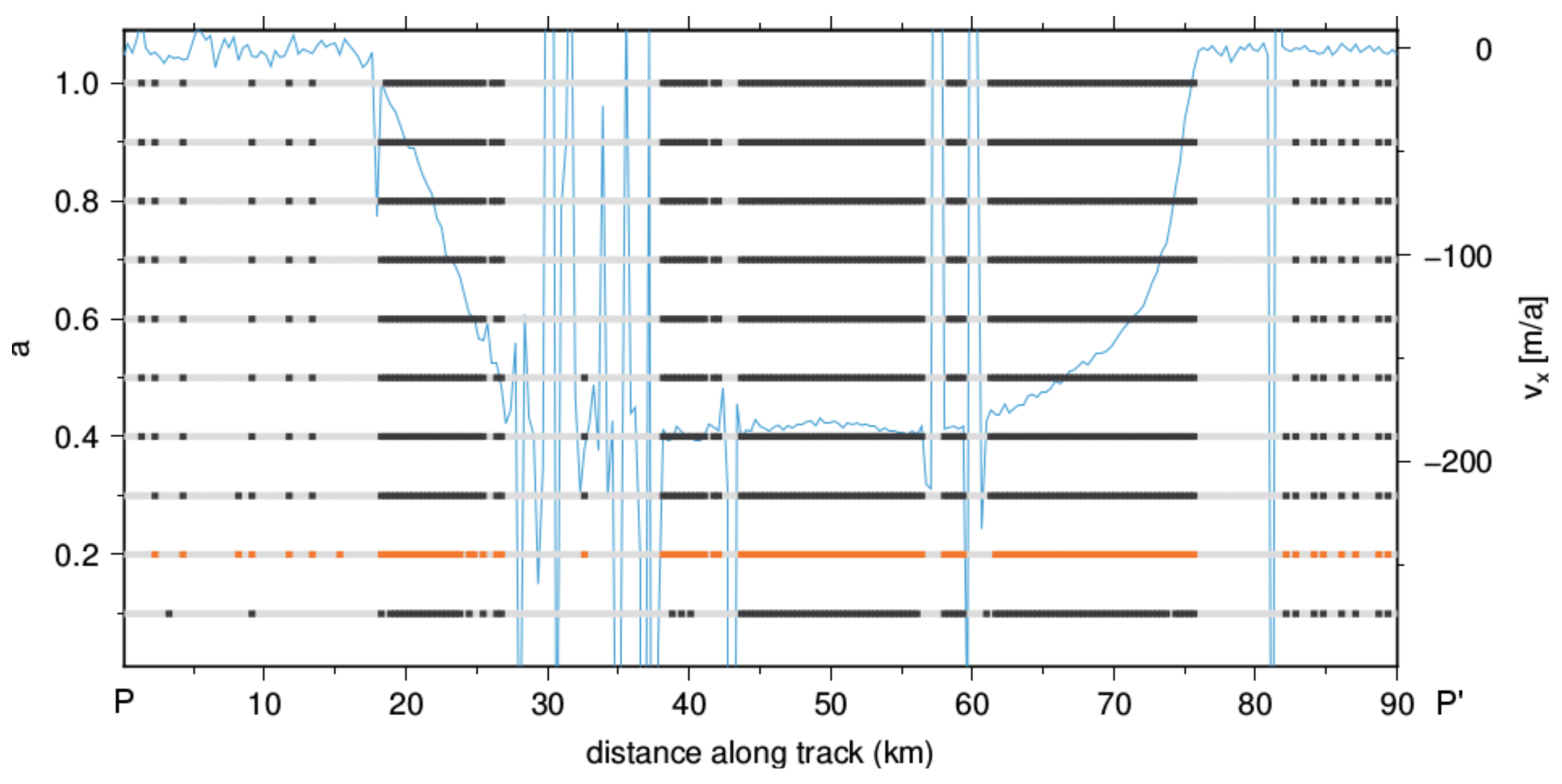
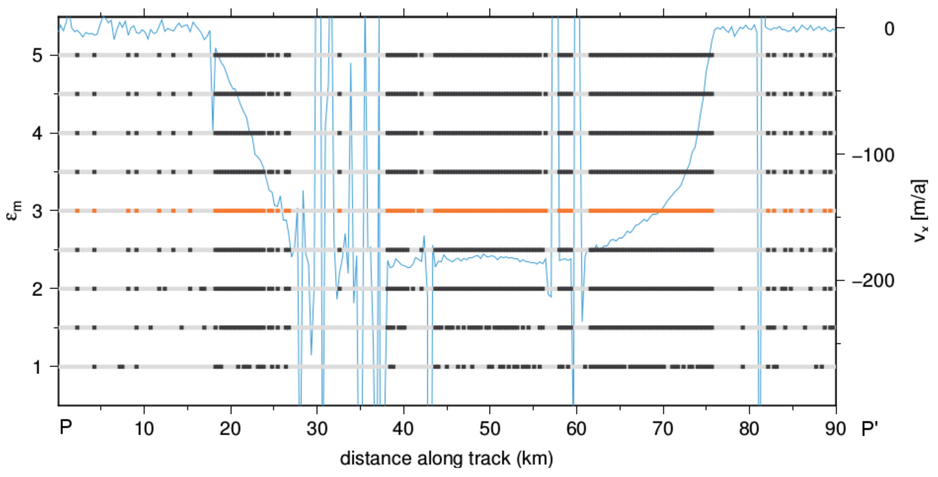
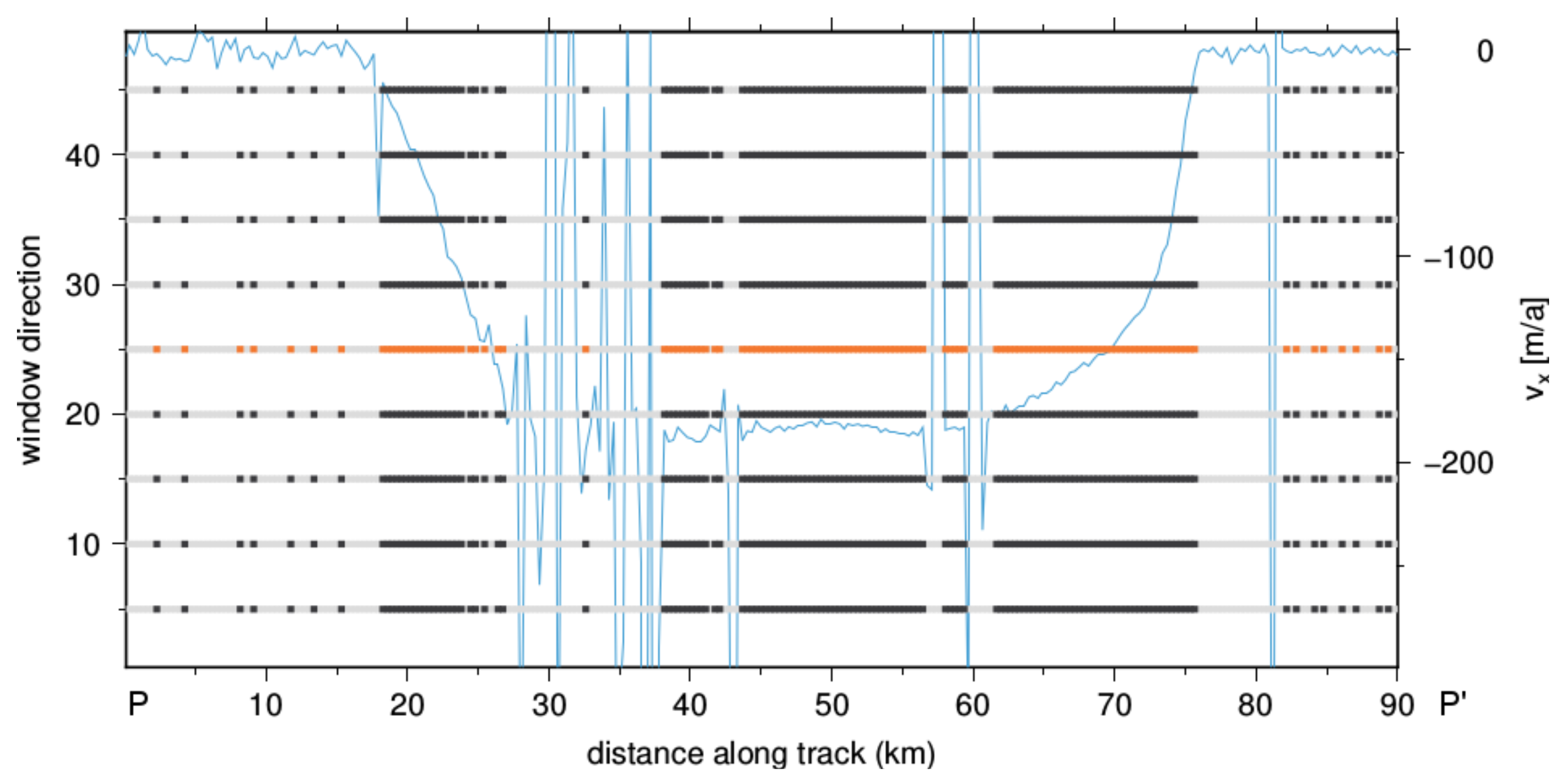
Here we present additional information on the sensitivity of the individual filter steps to their parameters. The graphs displayed in Figure A2, Figure A3, Figure A4, Figure A5 and Figure A6 are undermining the discussion in Section 3.2 and Section 4 and visualise the parameters used in our applications to glaciers in Greenland and Antarctica. Each figure displays (blue color, right y-axis) along a transect crossing a glacier and hence incorporate slow and fast moving glaciers and the shear zone in their transition. The different parameter values are shown as values along the left y-axis. In all cases, data points that have been removed appear in grey color, whereas data points that passed the filter are drawn as black points, or in orange color for those filter parameter setting that has been our setting in the applications to ice sheets within this study.
Figure A2.
Sensitivity of the first filter (smooth segments) to w. Data points that passed the filter are plotted as black points, while those that were removed are shown in gray color. The left y-axis represents the value of , while the right axis denotes the velocity. The selected value of is highlighted in orange. The blue line displays the original velocity in x-direction along the profile shown in Figure 3d.

Figure A3.
Sensitivity of the first filter (smooth segments) to a.

Figure A4.
Sensitivity of the first filter (smooth segments) to .

Figure A5.
Sensitivity of the second filter (median) to .

Figure A6.
Sensitivity of the third filter (directions) to .

References
- Joughin, I.; Smith, B.; Howat, I.; Scambos, T.; Moon, T. Greenland flow variability from ice-sheet-wide velocity mapping. J. Glaciol. 2010, 56, 415–430. [Google Scholar] [CrossRef]
- Fahnestock, M.; Scambos, T.; Moon, T.; Gardner, A.; Haran, T.; Klinger, M. Rapid large-area mapping of ice flow using Landsat 8. Remote Sens. Environ. 2015, 185, 84–94. [Google Scholar] [CrossRef]
- Nagler, T.; Rott, H.; Hetzenecker, M.; Wuite, J.; Potin, P. The Sentinel-1 Mission: New Opportunities for Ice Sheet Observations. Remote Sens. 2015, 7, 9371–9389. [Google Scholar] [CrossRef]
- Kääb, A.; Winsvold, S.; Altena, B.; Nuth, C.; Nagler, T.; Wuite, J. Glacier Remote Sensing Using Sentinel-2. Part I: Radiometric and Geometric Performance, and Application to Ice Velocity. Remote Sens. 2016, 8, 598. [Google Scholar] [CrossRef]
- Mouginot, J.; Rignot, E.; Scheuchl, B.; Millan, R. Comprehensive Annual Ice Sheet Velocity Mapping Using Landsat-8, Sentinel-1, and RADARSAT-2 Data. Remote Sens. 2017, 9, 20. [Google Scholar] [CrossRef]
- Yan, S.; Liu, G.; Wang, Y.; Ruan, Z. Accurate Determination of Glacier Surface Velocity Fields with a DEM-Assisted Pixel-Tracking Technique from SAR Imagery. Remote Sens. 2015, 7, 10898–10916. [Google Scholar] [CrossRef]
- Gray, A.L.; Mattar, K.E.; Sofko, G. Influence of ionospheric electron density fluctuations on satellite radar interferometry. Geophys. Res. Lett. 2000, 27, 1451–1454. [Google Scholar] [CrossRef]
- Wegmüller, U.; Werner, C.; Strozzi, T.; Wiesmann, A. Ionospheric Electron Concentration Effects on SAR and INSAR. Proceeding of the 2006 IEEE International Symposium on Geoscience and Remote Sensing, Denver, CO, USA, 31 July–4 August 2006; pp. 3731–3734. [Google Scholar]
- Rosenau, R.; Scheinert, M.; Dietrich, R. A processing system to monitor Greenland outlet glacier velocity variations at decadal and seasonal time scales utilizing the Landsat imagery. Remote Sens. Environ. 2015, 169, 1–19. [Google Scholar] [CrossRef]
- Seehaus, T.; Marinsek, S.; Helm, V.; Skvarca, P.; Braun, M. Changes in ice dynamics, elevation and mass discharge of Dinsmoor-Bombardier-Edgeworth glacier system, Antarctic Peninsula. Earth Planet. Sci. Lett. 2015, 427, 125–135. [Google Scholar] [CrossRef]
- Floricioiu, D.; Abdel Jaber, W.; Jezek, K. TerraSAR-X and TanDEM-X observations of the Recovery Glacier system, Antarctica. Proceeding of the 2014 IEEE International Geoscience and Remote Sensing Symposium (IGARSS), Quebec City, QC, Canada, 13–18 July 2014; pp. 4852–4855. [Google Scholar]
- Abdel Jaber, W. Derivation of Mass Balance and Surface Velocity of Glaciers by Means of High Resolution Synthetic Aperture Radar: Application to the Patagonian Icefields and Antarctica. Ph.D. Thesis, Technical University of Munich, Munich, Germany, 2016. [Google Scholar]
- Rignot, E.; Mouginot, J.; Scheuchl, B. Ice Flow of the Antarctic Ice Sheet. Science 2011, 333, 1427–1430. [Google Scholar] [CrossRef] [PubMed]
- Rignot, E.; Mouginot, J.; Scheuchl, B. MEaSUREs InSAR-Based Antarctica Ice Velocity Map; NASA DAAC at the National Snow and Ice Data Center: Boulder, CO, USA, 2011. [Google Scholar]
- Wessel, P.; Smith, W.H.F.; Scharroo, R.; Luis, J.; Wobbe, F. Generic Mapping Tools: Improved Version Released. Eos Trans. Am. Geophys. Union 2013, 94, 409–410. [Google Scholar] [CrossRef]
- Morlighem, M.; Rignot, E.; Mouginot, J.; Seroussi, H.; Larour, E. Deeply incised submarine glacial valleys beneath the Greenland ice sheet. Nat. Geosci. 2014, 7, 418–422. [Google Scholar] [CrossRef]
- Morlighem, M.; Rignot, E.; Mouginot, J.; Seroussi, H.; Larour, E. IceBridge BedMachine Greenland, Version 2; NASA DAAC at the National Snow and Ice Data Center: Boulder, CO, USA, 2015. [Google Scholar]
- Joughin, I.; Smith, B.; Howat, I.; Scambos, T. MEaSUREs Multi-year Greenland Ice Sheet Velocity Mosaic, Version 1; NASA National Snow and Ice Data Center Distributed Active Archive Center: Boulder, CO, USA, 2016. [Google Scholar]
- Rankl, M.; Kienholz, C.; Braun, M. Glacier changes in the Karakoram region mapped by multimission satellite imagery. Cryosphere 2014, 8, 977–989. [Google Scholar] [CrossRef] [Green Version]
- Mcnabb, R.; Hock, R.; O’Neel, S.; Rasmussen, L.; Ahn, Y.; Braun, M.; Conway, H.; Herreid, S.; Joughin, I.; Pfeffer, W.; et al. Using surface velocities to calculate ice thickness and bed topography: A case study at Columbia Glacier, Alaska, USA. J. Glaciol. 2012, 58, 1151–1164. [Google Scholar] [CrossRef]
- Mouginot, J.; Scheuchl, B.; Rignot, E. Mapping of Ice Motion in Antarctica Using Synthetic-Aperture Radar Data. Remote Sens. 2012, 4, 2753–2767. [Google Scholar] [CrossRef]
- Scherler, D.; Leprince, S.; Strecker, M.R. Glacier-surface velocities in alpine terrain from optical satellite imagery-Accuracy improvement and quality assessment. Remote Sens. Environ. 2008, 112, 3806–3819. [Google Scholar] [CrossRef]
- Burgess, E.W.; Forster, R.R.; Larsen, C.F.; Braun, M. Surge dynamics on Bering Glacier, Alaska, in 2008–2011. Cryosphere 2012, 6, 1251–1262. [Google Scholar] [CrossRef]
- Heid, T.; Kääb, A. Evaluation of existing image matching methods for deriving glacier surface displacements globally from optical satellite imagery. Remote Sens. Environ. 2012, 118, 339–355. [Google Scholar] [CrossRef]
- Neckel, N.; Loibl, D.; Rankl, M. Recent slowdown and thinning of debris-covered glaciers in south-eastern Tibet. Earth Planet. Sci. Lett. 2017, 464, 95–102. [Google Scholar] [CrossRef]
- Pritchard, H. Glacier surge dynamics of Sortebræ, east Greenland, from synthetic aperture radar feature tracking. J. Geophys. Res. 2005, 110, 13. [Google Scholar] [CrossRef]
- Strozzi, T.; Luckman, A.; Murray, T.; Wegmüller, U.; Werner, C. Glacier motion estimation using SAR offset-tracking procedures. IEEE Trans. Geosci. Remote Sens. 2002, 40, 2384–2391. [Google Scholar] [CrossRef]
- Jezek, K.; Floricioiu, D.; Farness, K.; Yague-Martinez, N.; Eineder, M. TerraSAR-X observations of the recovery glacier system, Antarctica. In Proceedings of the IEEE International Geoscience and Remote Sensing Symposium, Cape Town, South Africa, 12–17 July 2009; Volume 2, pp. 226–229. [Google Scholar]
Figure 1.
Performance test of the filter using an artificial velocity field: (a) Before filtering and (b) after filtering.
Figure 1.
Performance test of the filter using an artificial velocity field: (a) Before filtering and (b) after filtering.

Figure 2.
Sensitivity of the third filter (directional) to . Data points that passed the filter are plotted as black points, while those that were removed are shown in gray color. The selected value of (left vertical axis) is highlighted in orange. The blue line displays along the profile shown in Figure 3d.

Figure 3.
Velocities in x-direction of the Recovery Glacier, Antarctica: (a) Original data. (b) After the first filter step (smooth segments). (c) After the second filter step (median). (d) After the third filter step (directions). The upper left panel shows the locations of the tested regions: 1—fast flowing region, 2—shear margin, 3—region with line of outliers and 4—slow flowing region.

Figure 4.
Boxplots of the four test regions at Recovery Glacier. before (a) and after (b) filtering. before (c) and after filtering (d).
Figure 4.
Boxplots of the four test regions at Recovery Glacier. before (a) and after (b) filtering. before (c) and after filtering (d).

Figure 5.
Velocities in x-direction in a shear margin of the Recovery Glacier, Antarctica: (a) Original data. (b) After the first filter step (smooth segments). (c) After the second filter step (median). (d) After the third filter step (directions).
Figure 5.
Velocities in x-direction in a shear margin of the Recovery Glacier, Antarctica: (a) Original data. (b) After the first filter step (smooth segments). (c) After the second filter step (median). (d) After the third filter step (directions).

Figure 6.
Velocities in x-direction in a fast flowing region of the Recovery Glacier, Antarctica: (a) Original data. (b) After the first filter step (smooth segments). (c) After the second filter step (median). (d) After the third filter step (directions).
Figure 6.
Velocities in x-direction in a fast flowing region of the Recovery Glacier, Antarctica: (a) Original data. (b) After the first filter step (smooth segments). (c) After the second filter step (median). (d) After the third filter step (directions).

Figure 7.
Velocities in x-direction in a slow flowing region of the Recovery Glacier, Antarctica: (a) Original data. (b) After the first filter step (smooth segments). (c) After the second filter step (median). (d) After the third filter step (directions).
Figure 7.
Velocities in x-direction in a slow flowing region of the Recovery Glacier, Antarctica: (a) Original data. (b) After the first filter step (smooth segments). (c) After the second filter step (median). (d) After the third filter step (directions).

Figure 8.
Velocities in x-direction in a region with a line of outliers of the Recovery Glacier, Antarctica: (a) Original data. (b) After the first filter step (smooth segments). (c) After the second filter step (median). (d) After the third filter step (directions).
Figure 8.
Velocities in x-direction in a region with a line of outliers of the Recovery Glacier, Antarctica: (a) Original data. (b) After the first filter step (smooth segments). (c) After the second filter step (median). (d) After the third filter step (directions).

Figure 9.
Surface velocities of the Greenland Ice Sheet (magnitude): (a) Original data (b) Filtered data. (c) Removed data. The left panel indicates the locations of the tested regions: 1—Petermann Glacier, 2—subset of the North East Greenland Ice Stream (NEGIS).
Figure 9.
Surface velocities of the Greenland Ice Sheet (magnitude): (a) Original data (b) Filtered data. (c) Removed data. The left panel indicates the locations of the tested regions: 1—Petermann Glacier, 2—subset of the North East Greenland Ice Stream (NEGIS).

Figure 10.
Boxplots of the three regions in Greenland. (a) In x-direction before filtering. (b) In x-direction after filtering. (c) In y-direction before filtering. (d) In y-direction after filtering.
Figure 10.
Boxplots of the three regions in Greenland. (a) In x-direction before filtering. (b) In x-direction after filtering. (c) In y-direction before filtering. (d) In y-direction after filtering.

Figure 11.
of Petermann Glacier, Greenland: (a) Original data. (b) After the first filter step (smooth segments). (c) After the second filter step (median). (d) After the third filter step (directions). Circles and numbers indicate locations which are discussed in the main text.
Figure 11.
of Petermann Glacier, Greenland: (a) Original data. (b) After the first filter step (smooth segments). (c) After the second filter step (median). (d) After the third filter step (directions). Circles and numbers indicate locations which are discussed in the main text.

Figure 12.
of the NEGIS subset, Greenland: (a) Original data. (b) After the first filter step (smooth segments). (c) After the second filter step (median). (d) After the third filter step (directions).
Figure 12.
of the NEGIS subset, Greenland: (a) Original data. (b) After the first filter step (smooth segments). (c) After the second filter step (median). (d) After the third filter step (directions).


Table 1.
Statistical properties of the velocity in x- and y-direction before and after application of all three filter steps in the tested regions.
Table 1.
Statistical properties of the velocity in x- and y-direction before and after application of all three filter steps in the tested regions.
| Region | Component | Mean before [m a ] | Mean after [m a ] | Standard Deviation before [m a ] | Standard Deviation after [m a ] |
|---|---|---|---|---|---|
| Recovery Glacier (RG) | −49.83 | −60.65 | 222.00 | 99.49 | |
| −5.82 | −7.40 | 203.77 | 69.09 | ||
| RG slowflowing region | −13.44 | −16.84 | 111.34 | 6.62 | |
| −3.47 | −4.63 | 104.99 | 4.42 | ||
| RG fastflowing region | −518.72 | −530.76 | 243.28 | 144.13 | |
| −373.49 | −374.38 | 242.39 | 110.98 | ||
| RG line ofoutliers | −59.60 | −57.59 | 183.84 | 43.04 | |
| −8.01 | −15.02 | 169.18 | 20.10 | ||
| RG shear | −269.21 | −296.07 | 278.77 | 202.53 | |
| margin | −3.93 | 0.89 | 243.12 | 112.50 | |
| Greenland mosaic | −10.32 | −11.92 | 134.11 | 124.85 | |
| 2.53 | 3.41 | 100.06 | 90.86 | ||
| PetermannGlacier | −200.95 | −206.43 | 224.59 | 225.19 | |
| 568.97 | 586.79 | 474.42 | 472.45 | ||
| NEGIS subset | 176.43 | 179.93 | 246.22 | 243.5 | |
| 294.83 | 296.06 | 413.03 | 400.63 |
Table 2.
Number of data points before and after application of all three filter steps in the tested regions.
Table 2.
Number of data points before and after application of all three filter steps in the tested regions.
| Region | Points before | Points after | Percentage of Remaining Data Points |
|---|---|---|---|
| Artificial flow field | 49,000 | 39,906 | 81.44% |
| Recovery Glacier (RG) | 7,748,376 | 6,422,695 | 82.89% |
| RG slow flowing region | 563,242 | 442,413 | 78.55% |
| RG fast flowing region | 95,280 | 91,092 | 95.60% |
| RG line of outliers | 514,596 | 414,873 | 80.62% |
| RG shear margin | 140,551 | 121,734 | 86.61% |
| Greenland mosaic | 28,087,899 | 26,632,467 | 94.82% |
| Petermann Glacier | 1,036,193 | 989,318 | 95.48% |
| NEGIS subset | 805,170 | 576,362 | 71.58% |
© 2017 by the authors. Licensee MDPI, Basel, Switzerland. This article is an open access article distributed under the terms and conditions of the Creative Commons Attribution (CC BY) license (http://creativecommons.org/licenses/by/4.0/).
Share and Cite
MDPI and ACS Style
Lüttig, C.; Neckel, N.; Humbert, A. A Combined Approach for Filtering Ice Surface Velocity Fields Derived from Remote Sensing Methods. Remote Sens. 2017, 9, 1062. https://0-doi-org.brum.beds.ac.uk/10.3390/rs9101062
AMA Style
Lüttig C, Neckel N, Humbert A. A Combined Approach for Filtering Ice Surface Velocity Fields Derived from Remote Sensing Methods. Remote Sensing. 2017; 9(10):1062. https://0-doi-org.brum.beds.ac.uk/10.3390/rs9101062
Chicago/Turabian StyleLüttig, Christine, Niklas Neckel, and Angelika Humbert. 2017. "A Combined Approach for Filtering Ice Surface Velocity Fields Derived from Remote Sensing Methods" Remote Sensing 9, no. 10: 1062. https://0-doi-org.brum.beds.ac.uk/10.3390/rs9101062
Note that from the first issue of 2016, this journal uses article numbers instead of page numbers. See further details here.