Article

Phenocams Bridge the Gap between Field and Satellite Observations in an Arid Grassland Ecosystem

1
Jornada Experimental Range, USDA-ARS, P.O. Box 30003, MSC 3JER, Las Cruces, NM 88003, USA
2
Department Forest, Rangeland, and Fire Sciences, University of Idaho, Moscow, ID 83844, USA
3
Jornada Experimental Range, New Mexico State University, P.O. Box 30003, MSC 3JER, Las Cruces, NM 880033, USA
4
School of Informatics, Computing, and Cyber Systems and Center for Ecosystem Science and Society, Northern Arizona University, Flagstaff, AZ 86011, USA
5
Department Biological Science, The University of Texas at El Paso, El Paso, TX 79968, USA
*
Author to whom correspondence should be addressed.
Remote Sens. 2017, 9(10), 1071; https://0-doi-org.brum.beds.ac.uk/10.3390/rs9101071
Submission received: 20 September 2017 / Revised: 14 October 2017 / Accepted: 18 October 2017 / Published: 21 October 2017
(This article belongs to the Special Issue Land Surface Phenology )

Abstract

:
Near surface (i.e., camera) and satellite remote sensing metrics have become widely used indicators of plant growing seasons. While robust linkages have been established between field metrics and ecosystem exchange in many land cover types, assessment of how well remotely-derived season start and end dates depict field conditions in arid ecosystems remain unknown. We evaluated the correspondence between field measures of start (SOS; leaves unfolded and canopy greenness >0) and end of season (EOS) and canopy greenness for two widespread species in southwestern U.S. ecosystems with those metrics estimated from near-surface cameras and MODIS NDVI for five years (2012–2016). Using Timesat software to estimate SOS and EOS from the phenocam green chromatic coordinate (GCC) greenness index resulted in good agreement with ground observations for honey mesquite but not black grama. Despite differences in the detectability of SOS and EOS for the two species, GCC was significantly correlated with field estimates of canopy greenness for both species throughout the growing season. MODIS NDVI for this arid grassland site was driven by the black grama signal although a mesquite signal was discernable in average rainfall years. Our findings suggest phenocams could help meet myriad needs in natural resource management.

Graphical Abstract

1. Introduction

Phenology—the timing of seasonal life cycle events in plants and animals—is an integrative indicator of species’ responses to environmental conditions [1,2]. As such, spatiotemporal trends derived from phenological data (e.g., timing of initial growth, peak greenness, or flower and fruit production in plants) have been pivotal for addressing a range of research questions. These include but are not limited to plant and ecosystem responses to climate change [3,4,5,6], the potential for ecosystem change to modify ecosystem services [7,8], and the alteration of ecosystems following species invasions [9].
While the value of phenological information is increasingly realized, there remains a lack of research-supported knowledge on specific approaches for incorporating phenological information in management decision making [10,11]. This may be for lack of understanding how phenological data can support natural resource management [12]. Although both the National Climate Assessment and the U.S. Environmental Protection Agency recently established national phenological indicators based on the start of spring [13,14], actionable steps for tying phenological indicators to land management lags behind the rapid growth of phenology monitoring programs. Phenological data can inform natural resource management decisions that control the movement of livestock within or between grazing areas, to indicate optimum windows for ecosystem management practices (i.e., herbicide applications and harvesting seed for native plant propagation) and monitoring (e.g., [15]), and to supplement adaptive management strategies for wildlife and landscape conservation. In addition, phenological metrics such as the start and length of growing season can also be used to map land cover types or plant distributions [16] that aid remote assessments of landscape change [17,18]. While such management applications are broadly relevant, they are particularly relevant to the large expanses of arid and semi-arid landscapes in the western U.S. under federal stewardship.
There are several key challenges to monitoring and managing natural resources in arid and semi-arid ecosystems. First, the vast areal extent of arid landscapes with limited access pose logistical challenges for sampling. Second, many landscapes in arid regions are characterized by modest to low vegetation cover which commonly comprises a mix of herbaceous grass and woody vegetation that express different phenological patterns and resource use. In these cases, biophysical retrievals via satellite remote sensing can be challenging due to the high albedo of exposed soil [19], the aggregated phenological signals resulting from grass and woody plant species [20], and low signal-to-noise ratio with modest seasonal cycles resulting from low vegetation cover [21]. Third, in many arid ecosystems, standing non-photosynthetic vegetation is a prominent component of foliar cover [22,23]. This non-photosynthetic vegetation introduces variability in the dormant season signal and complicates retrieval of phenological data from remotely sensed imagery.
Phenological information has been collected in many ways that can be considered an observation hierarchy with data captured across a range of space and time scales. Methods and data range from satellite remote sensing to in situ field observations by volunteer citizen scientists and instrument-based observations of leaf chemistry for individual plants [21,24]. There is a pressing need to develop and characterize relationships between metrics at different levels of such an observation hierarchy to facilitate extrapolation between spatial and temporal scales, reveal detection limitations, optimize sampling efficacy relative to decision-making needs, and validate model outcomes [11,21,24].
Repeat photography from ground- or tower-based digital cameras (hereafter “phenocams”) can be used to derive oblique near-surface remote depictions of land surface condition. Seasonal metrics derived from high-frequency (i.e., multiple images day−1) phenocam images provide a link between satellite and field perspectives and have been used to refine phenological models for forested ecosystems in the eastern U.S. [25,26]. Use of images from near-surface phenocams can increase temporal resolution, broaden the spatial footprint of field observations, and reduce costs of field-based observations [27]. Utility of phenocam imagery has been demonstrated for capturing land surface phenology, seasonality in primary production for a range of plant functional types including deciduous broadleaf forest, evergreen needleleaf forest, and grasslands along with plant communities in the Great Basin Desert [27,28,29,30]. Phenocams have also been used to provide effective proxy data for canopy development, carbon flux, and gross primary production in forested ecosystems and temperate grasslands [21,31], but less is known of the strengths and limitations of this technology for capturing seasonal changes in photosynthetic activity in arid and semi-arid ecosystems.
In this study, we evaluate how greenness indices derived from phenocams and satellite imagery time series over a five-year period (2012–2016) compare to finer scale field observations of plant phenology and estimates of percent canopy greenness in a Chihuahuan Desert grassland. Specifically, the remote sensing metrics we examine are the green chromatic coordinate (GCC) from time series phenocam images and the Normalized Difference Vegetation Index (NDVI) from 250-m MODIS imagery. In particular, we evaluate the performance of phenocam-derived data to characterize the phenology of an arid upland grassland ecosystem using the following objectives:
(1)
describe the phenological profiles of co-existing grass and shrub species using field data and phenocam imagery;
(2)
assess how phenological metrics such as start, end, and length of growing season vary between phenocam imagery and field observations;
(3)
examine the relationship between growing season estimates of canopy greenness for grass and shrub species using field methods and phenocam imagery; and
(4)
explore how species-level phenological trends contribute to landscape-level greenness derived from both phenocam imagery and MODIS NDVI.

2. Materials and Methods

2.1. Study Site

The study was conducted on the Jornada Experimental Range (JER) in southern New Mexico (central coordinates: 32.589°N, 106.845°W). The JER was established in 1912 as a field research station focused on developing methods to mitigate grassland degradation that was prevalent in much of the western United States at the turn of the 20th century [32]. Long-term mean (1970–2016 reported from in situ meteorological data) annual rainfall is 233 mm with >50% of annual rainfall occurring from July to October. Like much of the southwestern U.S., there is high inter-annual variation in rainfall [33]. Mean temperatures range from 3.8 °C in January to 26.0 °C in July [34].
Environmental conditions over the study period ranged from drier to above-average rainfall. The first year of the study (2012) was the fourth consecutive year of below-average annual rainfall. The second and third years (2013–2014) experienced near average rainfall and were followed by 2015 with above-average rainfall (Figure 1). Vegetation cover reflected this inter-annual variability in rainfall, with field estimates of foliar cover ranging from 56% in 2012 to 77% in 2015.
Phenocams were installed at an upland grassland dominated by the C4 perennial grass Bouteloua eriopoda (hereafter “black grama”) on a Sandy ecological site R042XB012NM [35] with sandy soils. The study site has been protected from livestock since 1972 although plants are subjected to herbivory by rodents and lagomorphs. While vegetation at this site is dominated by C4 perennial grasses, it has undergone increases in the C3 deciduous shrub Prosopis glandulosa (hereafter “mesquite”) over the last 160 years [36,37]. This proliferation of woody plants at the expense of perennial grasses has been observed in many drylands globally [38].
Black grama and mesquite represent different plant functional groups with contrasting life history characteristics, rooting depths, and responses to rainfall. From long-term data collected at this site, mesquite initiates growth in the early spring prior to the summer monsoon season (July–September). In contrast, black grama is known to initiate growth in the early spring but not reach peak greenness and production until summer rains fall in early July [39]. Black grama roots reach approximately 50 cm in depth while mesquite roots can extend laterally several meters and to depths greater than 5 m below the soil surface, allowing access to deeper soil moisture, thereby permitting the species to better avoid effects of drought [40,41].

2.2. Phenology Observations

We consider two classes of phenology metrics or phenometrics and highlight their utility in the context of natural resources management. Event-based metrics mark points of the growing season (e.g., start, peak, or end), whereas time-series metrics characterize sequential development over a growing season (e.g., plant canopy development; Denny et al. [42]). Event-based phenology metrics, such as “date of first flower” constitute the majority of phenology records and are important indicators of climate change [43], and for the management of crop systems [44], and the evaluation of year to year variability and identity of environmental drivers e.g., [45]. In contrast, intensity metrics (e.g., percent of canopy that is green) provide a link to temporal dynamics of CO2 flux and primary productivity e.g., [31] that are important for making decisions about grazing herd migration and the timing of field efforts to characterize forage or land surface condition.

2.2.1. Field

Field observations of phenological status for five individuals (hereafter, “focal plants”) of black grama and mesquite were made weekly using standardized protocols for event and intensity metrics developed by the USA National Phenology Network (USA-NPN) [42]. The intensity metric for leaves involved field observers visually estimating the percentage of live canopy containing unfolded green leaves using categorical rankings defined in the USA-NPN protocols. Measurements began 20 May 2012 and entailed assigning each focal plant to one of seven categories: 0%, 1–4%, 5–24%, 25–49%, 50–74%, 75–94% and 95–100%. Prior to May 2012, we implemented USA-NPN event metrics to characterize phenology.

2.2.2. Phenocams

Landscape-scale digital images in this study were acquired using two digital camera systems to compile the five-year time series. Phenocams were placed at locations adjacent to focal plants to prevent disturbance associated with foot traffic for field data collection in the camera fields of view (Figure 2). In February 2012, we deployed a stand-alone digital camera (Plantcam 1.0 MP by Wingscapes; hereafter “plantcam”) on a tripod situated two meters above the surface with an oblique view angle. We followed Phenocam Network protocols, with two exceptions. First, the Plantcam camera we deployed was not the recommended camera; thus some configuration settings in the protocol did not apply. Second, dust flux is high at this study location [46] and precluded the use of a reference panel as a non-variant feature in the field of view. Photos were initially acquired at 30-min intervals between 11:00 and 14:00 MST. However, to implement percentile regression using GCC from all images to derive a daily value [27], we increased the photo acquisition interval to 5 min between 11:00 and 13:00 on 29 October 2012 and maintained this interval through the remainder of the study.
In February 2014, we deployed a networked digital camera (StarDot Netcam SC 1.3 MP [StarDot, Buena Park, California, USA]; hereafter “netcam”) mounted atop a tower 6 m above the ground surface with an oblique view angle of approximately 20 degrees from horizontal (Figure 2). The netcam was configured as part of the PhenoCam Network and acquired images every 15 min between 10:00 and 16:00 through the remainder of the study.
Sonnentag et al. [27] compared performance of different digital cameras (including those used in this study) and suggested that derived metrics are not adversely affected by differences in camera configuration. For both phenocam systems, the camera field of view was fixed for the duration of the study. This is an important requirement for automated processing of phenocam images. The two camera systems described above were located ca. 100-m apart and were oriented in the same cardinal direction to represent similar views of the plant community. However, the digital numbers for color channels were not calibrated across cameras. Thus, we focused on normalized index values for comparison and assumed that the growing season metrics derived (describe below) for the two camera systems were equivalent [27]. Data from the plantcam were used for 2012 and 2013 while the netcam was used for 2014, 2015 and 2016 growing season metrics. Focal plants on which field observations were made occurred adjacent to but not in the field of view of the two cameras.

2.2.3. Phenocam Image Processing

Because our goal was to identify species-specific phenological trends and relate these to satellite time series, we identified regions of interest (ROIs) for three categories: (1) black grama; (2) mesquite; and (3) landscape. ROIs were hand-digitized to delineate objects by which the digital numbers—values that quantify the intensity or brightness of a pixel in the image – are summarized. We selected two mesquite shrub ROIs (mean size of 4.1 m2) in each camera field of view and identified the largest homogeneous patches of the dominant black grama grass (1–3 patches with mean size of 166.5 m2; see Figure 2A,B). We also selected a representative ROI for each camera field-of-view to represent the landscape and extracted seasonal metrics (start, end, date of peak greenness). Size of the landscape ROI ranged from 1156 m2 for the plantcam to 7265 m2 for the netcam (Figure 2C).
Greenness metrics were derived from phenocam digital images by summarizing digital numbers for red, green, and blue (i.e., RGB) channels of pixels in a specific ROI (Figure 2, Equation (1)). Two greenness indices in the RGB color space have been widely used for phenocam imagery: Excess Green and Green Chromatic Coordinate GCC [27]. We opted to use the GCC metric because it has been shown to be less influenced by differences in illumination and camera properties [27]. GCC is derived by dividing the digital numbers of the green color channel by the sum of digital numbers for red, green, and blue color channels:
G C C = D N G D N R + D N G + D N B
where DN represents the digital number for the green, red, and blue channels [21]. GCC values reported hereafter represent the mean value for all pixels within the mesquite shrub, black grama, and landscape ROIs for each camera time series.
All images from each day were used to derive daily GCC values for each ROI and the 90th percentile for all daily images was calculated. To reduce noise from changes in illumination, a three-day window was applied by assigning the 90th percentile of all daytime values of GCC to the window center day. By calculating values over a three-day window, we smoothed out noise in the data while maintaining high enough temporal frequency to precisely identify when change occurs in the GCC time series [27].
To compare growing season metrics from the two camera systems, we normalized the GCC values for each camera separately following normalization procedures from Keenan et al. [47] as follows. For each ROI we selected minimum and maximum GCC from the three-day smoothed values for each annual growing season. Annual minimum and maximum GCC values were averaged and three-day GCC values (x0 in Equation (2)) were normalized relative to the mean annual maximum and minimum for each ROI (xmax and xmin in Equation (2)).
x n o r m = x 0 x m i n x m a x x m i n

2.3. Derivation of Seasonal Metrics

2.3.1. Field Phenophase Observations

Seasonal event metrics from field observations denoted the start of each phenophase with a temporal uncertainty of seven days between field visits. Start of season (SOS) for black grama and mesquite plants represented the date unfolded leaves were first recorded for each plant each year. End of season (EOS) was defined as the last date that percent green canopy was judged to be greater than zero. Growing season length (GSL) was the number of growing season days between SOS and EOS. Dates reported were the mean of the five focal plants. The intensity metric for canopy greenness through the growing season was reported as the categorical ranking of percent green canopy.

2.3.2. Phenocams (Timesat)

We used Timesat v3.2 [48], a widely-used software program for extracting seasonal metrics from remotely sensed time series, to compare SOS and EOS dates based on smoothed three-day GCC for the three phenocam ROIs. Black grama and mesquite seasonal metrics from Timesat were compared with field dates while landscape seasonal metrics were compared to MODIS NDVI (Figure 3). We used the Savitsky–Golay model [48] with seasonal parameter set to 0.5 (default) and amplitude method and evaluated outputs using four thresholds: 10%, 15%, 20% and 25% representing percentage of annual amplitude. In Timesat, the seasonal parameter indicates the number of seasons per year. We found that a seasonal parameter of 0.5 offers the best logistic model fit in arid landscapes with high interannual variability in primary production. The percent annual amplitude threshold is set in the graphical user interface. In some instances (particularly for the lowest 10% threshold), the Timesat algorithm identified the EOS date in the following calendar year. If the EOS date was less than DOY 15 of the following year, the EOS date was set to 365; otherwise, the EOS date was noted as NA in the Results (see Table A1 and Table A2).

2.3.3. MODIS NDVI (Timesat)

We generated dates for start, end, and peak season with Timesat using MODIS NDVI values from the 250-m (MOD13Q1) data product for years 2012–2016 to coincide with phenocam data coverage. NDVI values were averaged for the 2 × 2 MODIS pixel window that encompassed the focal plants and the fields of view for both phenocams.

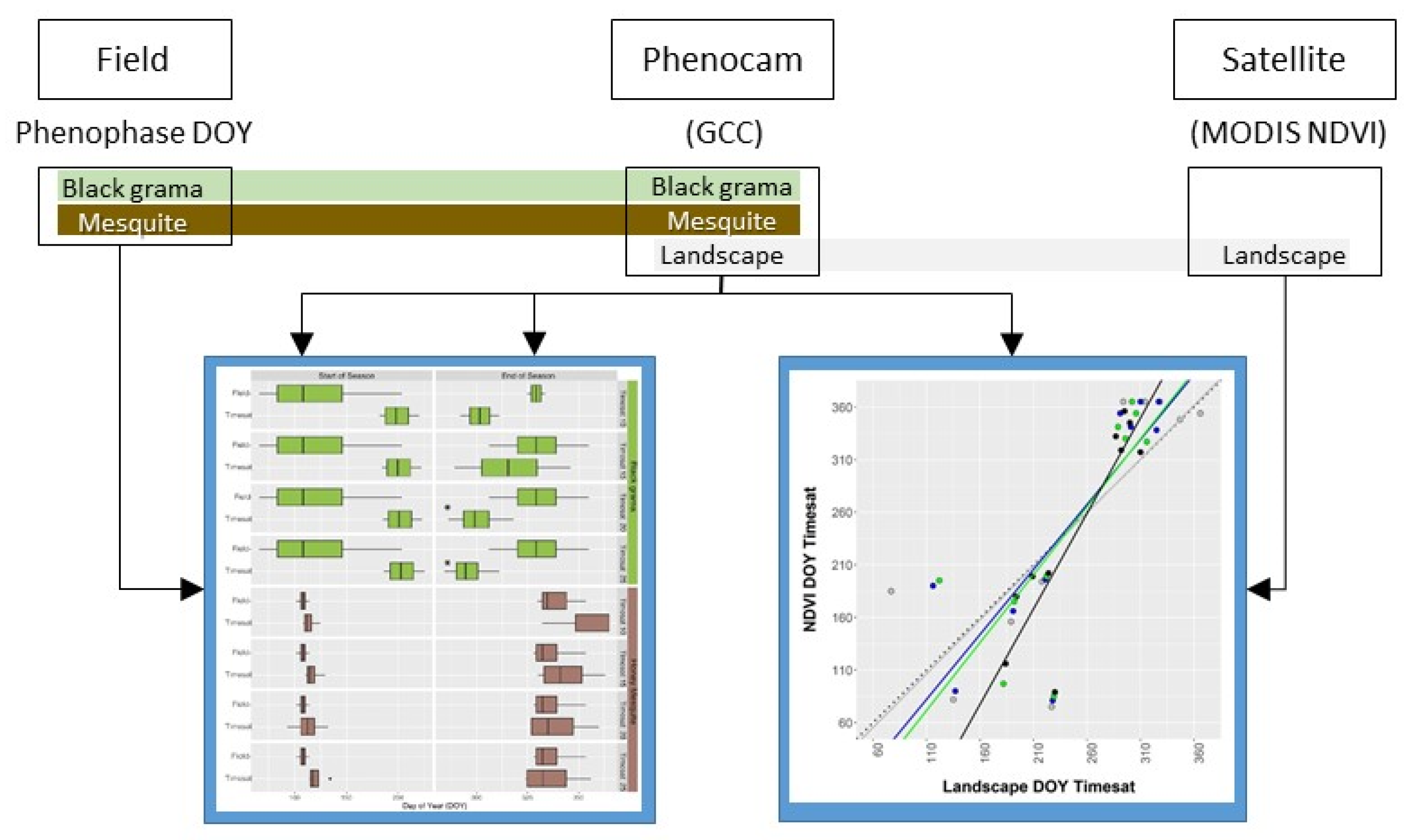
2.4. Data Analysis—Metric Comparisons

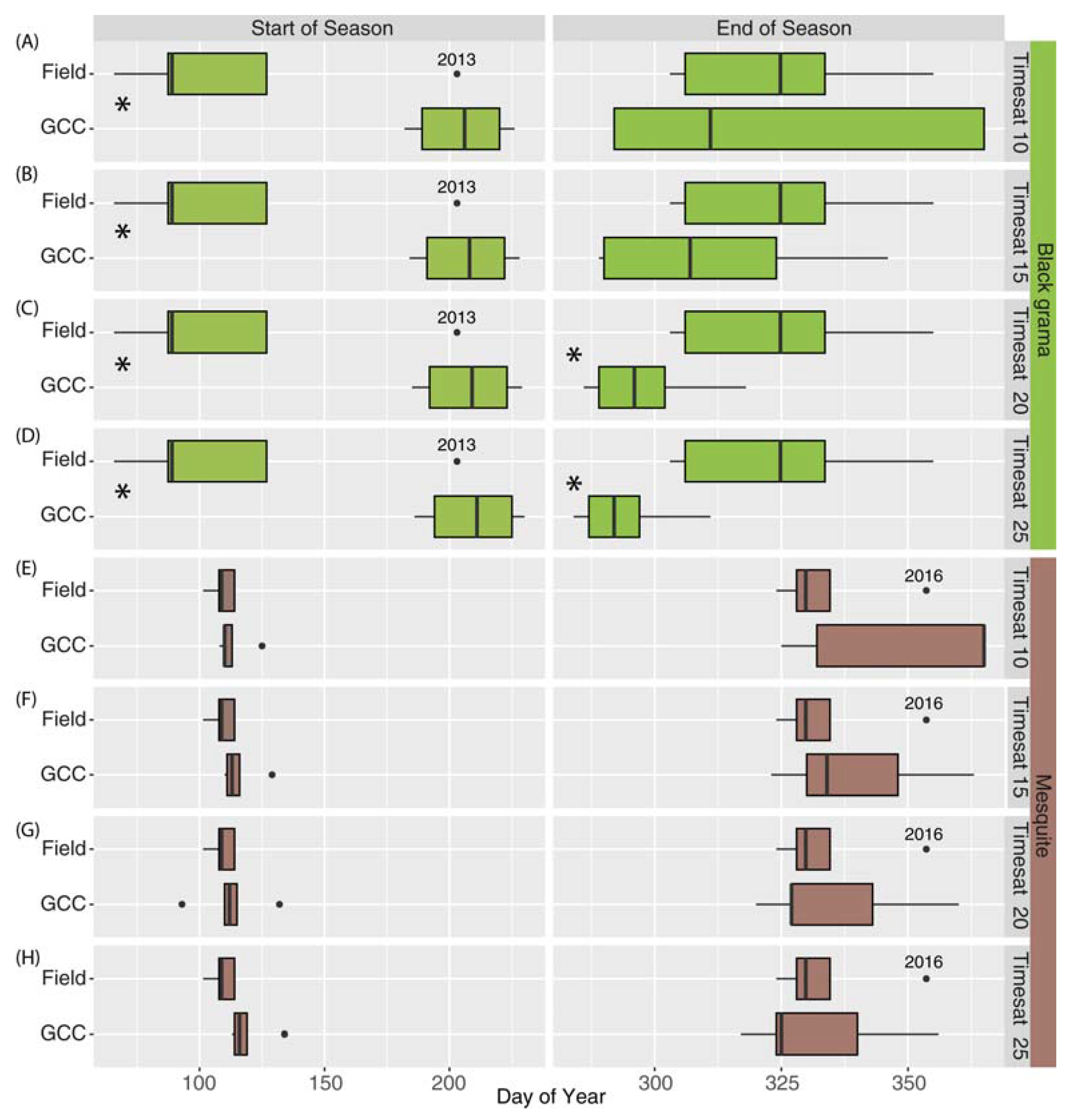
2.4.1. Seasonal Metrics (Field vs. PhenoCam, Objective 2)

Camera-derived metrics for SOS and EOS using black grama and mesquite ROIs via Timesat were compared to field-based dates for SOS and EOS using paired t-tests. In addition, we report root mean squared error (RMSE) to quantify the spread or bias in the SOS and EOS metrics. We evaluated the four seasonal amplitude thresholds (10%, 15%, 20%, and 25%).

2.4.2. Canopy Greenness (Field vs. Phenocam, Objective 3)

Growing season patterns in greenness from GCC offer information beyond event-based SOS and EOS dates. Correlations between categorical field estimates of percent live canopy greenness with phenocam GCC values were evaluated using Spearman rank correlation. Percent canopy greenness category for five black grama and five mesquite focal plants were averaged for comparison with the 90th percentile GCC value for a given field observation date.

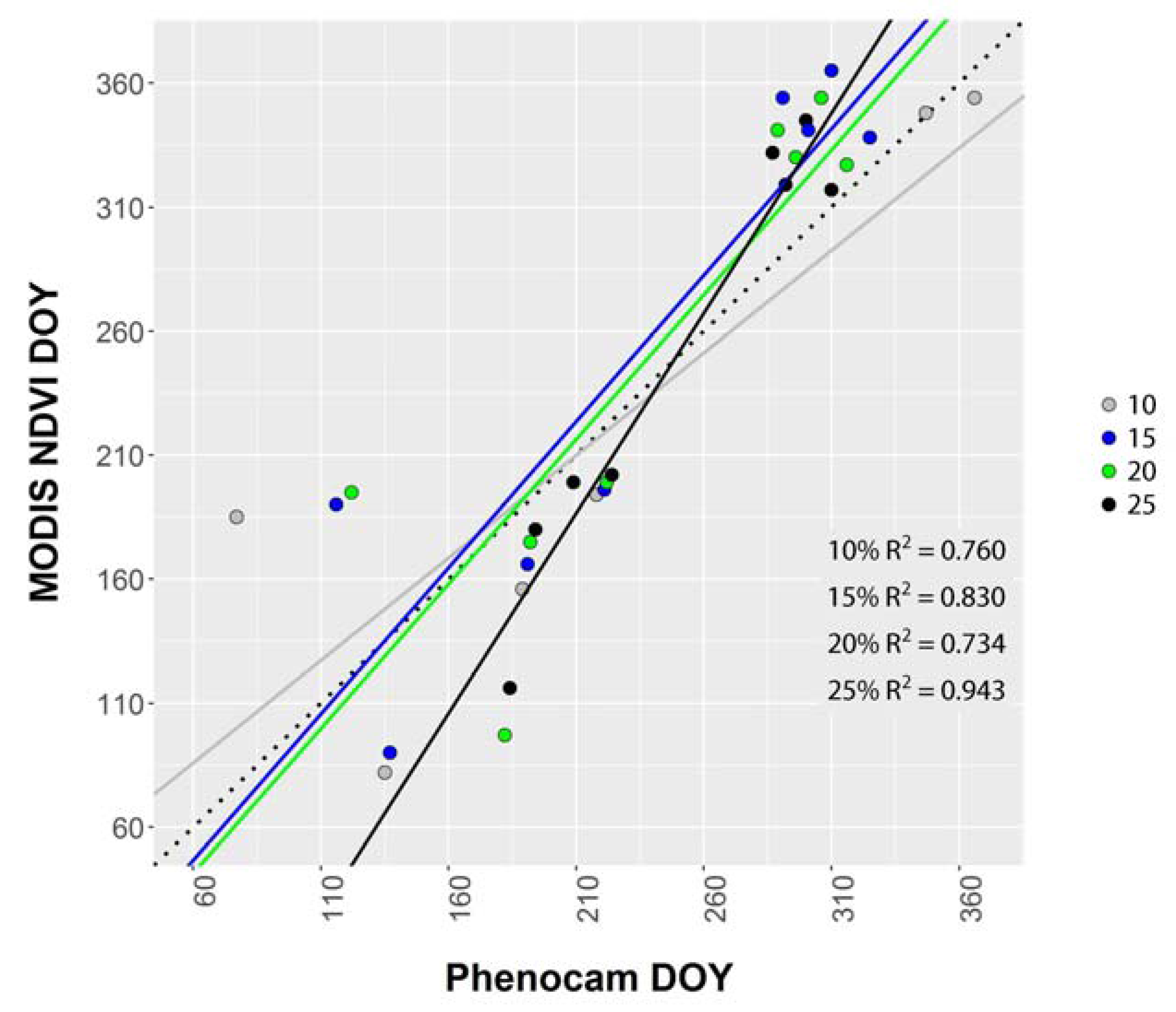
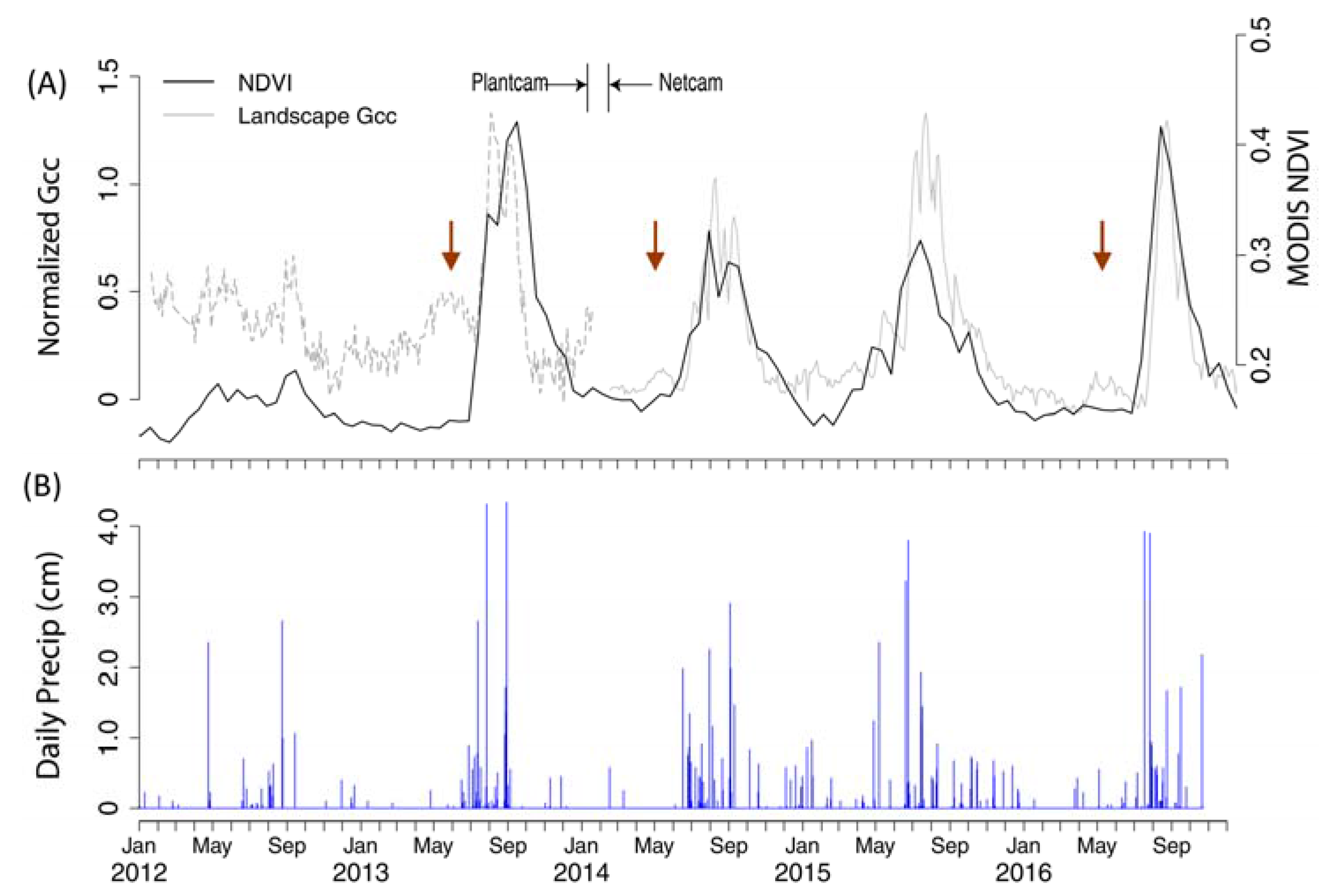
2.4.3. Landscape Greenness (Phenocam vs. MODIS, Objective 4)

Patterns in landscape greenness from NDVI and GCC were evaluated using seasonal metrics and landscape greenness data over the time series. First, we quantified the relationship between SOS and EOS dates from NDVI and phenocam GCC for the landscape ROI using Timesat. Second, we qualitatively evaluated landscape patterns in greenness throughout the growing season in the context of the black grama and mesquite greenness patterns (see Figure 3).

3. Results

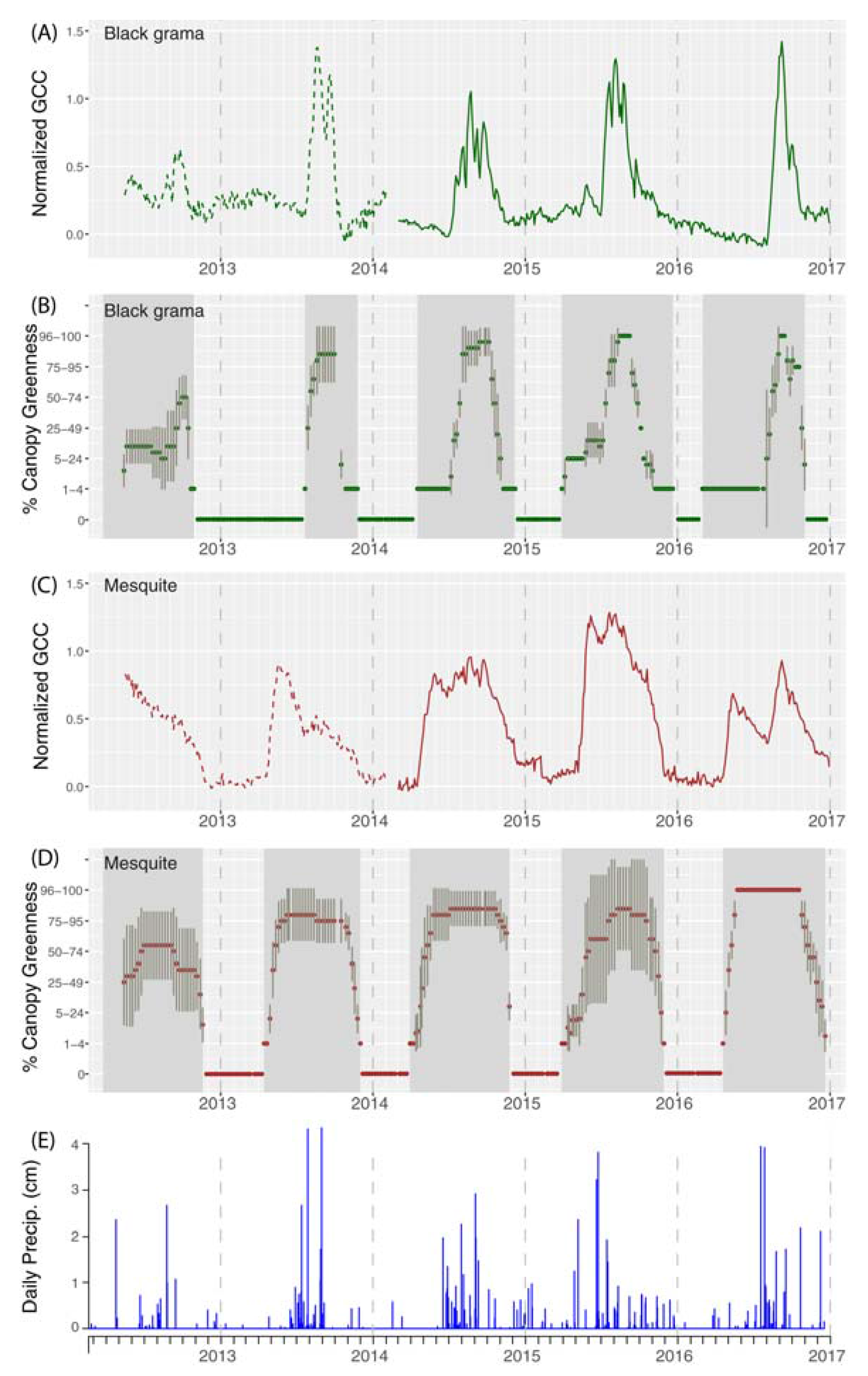
3.1. Phenological Profiles (Field and Phenocam, Objective 1)

Field data revealed distinct seasonal patterns in grass and shrub phenology that differed in timing and interannual variability. Field observations indicated growing season length for black grama ranged from 122 days in 2013 to 266 days in 2015 and for mesquite from 210 days in 2012 to 240 days in 2016. Black grama exhibited high inter-annual variability in the SOS ranging from Day 66 in 2016 to Day 203 in 2013 while SOS for mesquite was more consistent, ranging from Day 101 in 2014 to Day 114 in 2012 and 2016 (Table 1). Both species generally exhibited similar mean EOS dates in mid-November to December (Days 308 to 355) although black grama retained basal greenness through late December in 2015 (Table 1).
Black grama also demonstrated higher variability among plants than mesquite in field-observed SOS and EOS. In 2014, black grama focal plants were most variable in both SOS and EOS dates. In 2013 and 2015, all focal black grama plants unfolded leaves (SD = 0.0) on days 203 and 89, respectively. Synchronous transitions for all five focal plants (i.e., SD = 0) occurred half as often for mesquite and only for EOS dates (Table 1). Field-observed dates for mesquite SOS and EOS were most variable in 2015, while in the same year, all black grama focal plants had the same SOS and EOS dates.
Species-specific seasonal GCC patterns from phenocams demonstrated distinguishable differences in periodicity in greenness for C4 black grama and the deciduous C3 mesquite. We found a consistent peak in mesquite greenness in spring (April to May) and in black grama greenness in late summer (August). Black grama growing seasons via phenocams exhibited greater year-to-year variation in peak greenness with shorter growing season for black grama that for mesquite (Figure 4). The seasonal cycle in GCC for mesquite was typified by a rapid rise to peak green in April followed by a decline in greenness over summer with an occasional second peak (e.g., 2016) and a steep decline in autumn to a consistent minimum in winter. In contrast, the seasonal cycle in GCC for black grama was characterized by a steep rise in early summer (ranging from early July to mid-August) and high frequency pulses in greenness that follow precipitation events or pulses with a lag of 3–7 days (Figure 4).
Spearman rank correlations between field estimates of greenness and phenocam-derived greenness were strongly positive for both species. Black grama GCC values were significantly correlated with field greenness (r = 0.644, p < 0.0001 for plantcam GCC, n = 160 and r = 0.609, p < 0.0001 for netcam GCC, n = 178). Correlations between mesquite GCC values and field estimates were somewhat higher (r = 0.760, p < 0.0001 for plantcam GCC, n = 160; and r = 0.735, p < 0.0001 for netcam GCC, n = 178) than for black grama.
Annual patterns in field and camera greenness captured dormancy as well as greenness dynamics. Both species exhibited rapid increases in GCC with mesquite SOS consistently occurring in May and black grama mostly occurring in July; these patterns in canopy greenness were reflected in field observations (Figure 4B,D). The muted response in seasonal greenness in the 2012 drought year—both from field and phenocam perspectives—was more prominent for black grama than for mesquite (Figure 4). Patterns and correlations indicated GCC reflects field-observed greenness better for mesquite than black grama. The lowest level of percent green canopy for grasses was not captured by the phenocams as indicated by the periods such as May–July 2014 and March–July 2016 (Figure 4A,B). Coincidently, mesquite phenocam GCC captured fine-scale fluctuations in canopy greenness that were not captured with field-based estimates at the high (96–100%) canopy greenness as with May–September 2016 (Figure 4C,D).

3.2. Metric Comparisons

Seasonal Metrics (Field vs. Phenocam, Objective 2)

Overall, there was good correspondence between field and phenocam-derived metrics for SOS and EOS from Timesat although correspondence was greater for mesquite than for black grama. Paired t-tests at alpha = 0.05 denoted significant differences for black grama SOS dates with RMSEs ranging from 105.4 to 109.2 days using 10% and 25% thresholds, respectively (Figure 5A–D, Table 2). EOS dates for black grama estimated with Timesat were closer to those estimated via field observations with RMSEs ranging from 22.6 to 32.8 days using 15% and 25% thresholds, respectively (Table 2). Black grama exhibited high inter-annual variability in field SOS; GCC SOS dates were consistently later while EOS dates via GCC are earlier demonstrating a better fit and lower range in RMSE (Figure 5). In contrast, the correspondence between field and phenocam GCC SOS and EOS for mesquite was high. RMSE values for mesquite SOS ranged from 8.6 to 13.6 days using 10% and 25% thresholds, respectively while EOS ranged from 8.2 to 16.3 days using 25% and 10% thresholds, respectively (Table 2). For a given Timesat threshold to estimate mesquite SOS and EOS, 15% yielded RMSE values of 10.6 and 9.9, respectively (Figure 5, Table 2). Based on t-test and RMSE results, we report Timesat metrics for the 15% seasonal threshold for black grama and mesquite henceforth.
Seasonal metrics for both species varied from year to year. The range in black grama SOS via phenocams was later and narrower (DOY 191–228; Table A1) than was the range in field observed SOS (DOY 66–203; Table 1, Figure 4B). Both black grama and mesquite demonstrated similar EOS dates in mid-November to December. Mesquite EOS via phenocams ranged from Day 323 to Day 363, while black grama EOS ranged from Day 289 to Day 346 (Table A1).

3.3. Landscape Greenness (Phenocam vs. MODIS)

Patterns in landscape GCC tracked NDVI greenness as indicated by significant high R2 values for all four seasonal thresholds. The 25% threshold produced the highest R2 value (R2 = 0.943, Figure 6) but it also deviated most from the 1:1 line. Conversely, the 10% seasonal threshold corresponded most closely to the 1:1 line and produced a lower R2 value of 0.760. The lowest threshold (10%) was problematic for extracting SOS and EOS dates from MODIS imagery using Timesat. This was especially so during the drought year 2012 that had a muted NDVI response. For this reason, we excluded 2012 SOS and EOS dates from the 10% threshold regression. SOS occurred over a larger range of dates than did EOS for both NDVI and landscape GCC (Figure 6). The range in SOS dates for landscape GCC coincide with the pattern for black grama GCC (Figure 5A–D). RMSE values indicated the 25% seasonal amplitude threshold resulted in the lowest absolute difference between landscape GCC and MODIS NDVI for SOS (36.8 days) and EOS (34.7) metrics (Table 3).
Landscape GCC growing season patterns were evaluated in the context of species phenological profiles. When GCC profiles were examined in concert, the landscape pattern was dominated by the black grama response. This is most apparent by the muted landscape GCC response in the 2012 drought year, as noted above in Figure 4A for black grama. Interestingly, the peak in mesquite greenness that occurs annually in April or May was reflected in small increase in landscape GCC denoted with brown arrows in Figure 7 in 2013, 2014 and 2016, although this was not evident in the NDVI time series. Mesquite constitutes low cover at this site (approximately 6% foliar cover estimated in 2015) yet its phenological signature was reflected in the landscape phenocam GCC ROI seasonal profile in three of five years (brown arrows in Figure 7).
Land surface phenology from MODIS NDVI represents the aggregated response of species within a 6.25 ha footprint of a given MODIS pixel. As with field and phenocam estimates, variation in the date of NDVI SOS reflected the pattern of black grama green-up (Figure 4A and Figure 7A). In all years but 2012, differences in dates of peak GCC and NDVI were less than the 16 days, the interval over which a given pixel value can occur via the 16-day MODIS image compositing process, showing good correspondence.

4. Discussion

Phenology is sensitive to variation in weather and climate, and it also controls the seasonality of many ecosystem processes [5,6]. Therefore phenology monitoring programs can provide important information about ecosystem function and associated ecosystem services, which can contribute to improved land management practices [11]. We examined patterns in plant phenology in an arid grassland ecosystem using three observation platforms—ground, near surface digital cameras, and satellite—to assess the performance and relative utility of each for management applications.

4.1. Species Phenology Profiles

Understanding distinguishing characteristics of phenological profiles for dominant plant species or functional groups can augment interpretations of land surface phenology derived from satellite remote sensing. C4 grass and C3 shrub species exhibit markedly different phenological patterns that were consistent between both field and phenocam observations. Kemp [39] reported patterns in the timing of vegetative and reproductive phenophases for these species between 1978 and 1980 at a nearby site. Our field data concur with those of Kemp [39] who reported consistent timing of SOS for mesquite in early April and EOS dates ranging from the end of October to the end of November. Variable start times for black grama ranged from late July in 1978 to the end of March in 1980 and EOS dates ranged from mid-October to early November. Phenological patterns for black grama were more closely tied to precipitation while those for mesquite were less variable in timing and seemingly not tied to precipitation. The inflection point marking the onset of senescence to the EOS was similar for the two species. Given differences in rooting depths for grass and shrub species and rates of dry down across the soil profile, soil moisture seems unlikely to trigger senescence. We hypothesize that EOS may be triggered by changes in temperature or day length; future research is needed to test this hypothesis.
Seasonal patterns in grass and shrub greenness appear to reflect different responses to environmental conditions both within and among years. The growing season length in 2015 derived from the phenocam was the longest for black grama and the shortest for mesquite (Table A1). This contrast in the species’ responsiveness to the same environmental conditions—expressed in terms of differences in SOS and EOS—supports the theory of temporal niche partitioning or time as a niche axis [9]. Previous studies have proposed that phenology may explain differences in shrub and grass colonization [37] and differences in aboveground primary production following experimental manipulations of rainfall amount and variability [49]. Our findings further support the concept of temporal niche partitioning; however, experimental approaches are needed to achieve insights regarding mechanism.
High inter-annual variability in rainfall is a trait of many arid and semi-arid ecosystems and both phenocam and field metrics revealed inter-annual differences in seasonality for grass and shrub species. Species responses to variable rainfall are reflected by the muted NDVI signal in the 2012 drought year that corresponded to the black grama GCC response and low aboveground biomass at this site in 2012 (see Figure 4 in [50]). Despite high inter-annual rainfall variability in this study, seasonal cycles in GCC reported herein share characteristics of seasonal patterns reported for comparable plant functional types from more mesic systems sensu [20,27]. Generally, GCC patterns for deciduous mesquite shrubs are more conspicuous and are easily detected with tower-mounted digital cameras than those for black grama grasses. The mesquite GCC signal followed a similar pattern for deciduous tree species in New England described by Sonnentag [27] that is typified by a rapid rise in peak green in the spring followed by continuous decline over summer and a steep decline in autumn to a consistent minimum in winter. One notable difference in the mesquite GCC pattern at this site was the tendency for mesquite to exhibit more than one peak in greenness following the initial flush in spring as seen in August 2016 presumably due to high precipitation in July. The bimodal response in mesquite greenness indicates that while mesquite SOS is relatively unaffected by precipitation, canopy dynamics during the growing season dynamics can be greatly influenced by precipitation and the subtlety of those canopy dynamics is more readily revealed by GCC than by field observations of canopy greenness. In contrast, the GCC pattern for black grama was marked by a rapid response following precipitation, which has been noted in other C4 grasslands [20,51]. While the most consistent period of rainfall at this site occurs in early July, the C4 black grama GCC signal at this site tracks rainfall that occurred outside the monsoon season (Jul to Sep) although C4 responses to precipitation is likely limited by minimum temperature thresholds [52,53]. The pattern of high variation in grass green-up responses has been noted in other savanna and shrubland systems [20,30] in the western U.S.

4.2. Comparison of Phenology Metrics across Platforms

Phenocams offer the capacity to bridge disparate data sets that originate at distinct levels within an observation hierarchy [11,54]. Others have noted the inherently scale-dependent nature of phenology and the challenges associated with capturing the appropriate phenomenon using metrics that range in measurement scale (ordinal field measures to interval surface reflectance), positional and temporal accuracy, etc. [24,54]. We demonstrated a capability to characterize patterns at the level of individual plants and integrate plant responses over a larger area more commensurate with moderate spatial resolution satellite imagery in an arid environment. Key to developing robust scaling relationships is identifying and eliminating sources of uncertainty that can be controlled (e.g., species-specific patterns) and basing interpretations on the best available data.
Vegetation canopy development is important for carbon cycling, primary productivity, preventing soil erosion, and functioning as a source of shade and species habitat. Intensity phenological metrics (i.e., percent canopy with unfolded leaves) capture canopy development and offer additional information from event-based metrics (i.e., date of first unfolded leaves, SOS). Comparison of the intensity metric for field-estimated percent canopy with unfolded green leaves with time series GCC circumvented bias introduced by models used to derive seasonal metrics such as SOS or EOS. Phenocam GCC yielded significant positive correlations with weekly field estimates of percent of canopy with unfolded green leaves, thereby effectively increasing the temporal resolution of resource-intensive weekly measurements. In addition, GCC appears to capture mesquite canopy dynamics not captured by weekly field estimates of percent canopy with unfolded green leaves that may reflect finer scale (i.e., leaf level) energy exchange [28,29].
Landscape GCC patterns depict the aggregated response of all species within the phenocam field of view and are most suitable for comparison with MODIS NDVI. The species-specific responses from the phenocams allow evaluation of which species are driving the GCC signal for the landscape, and worked well in this study. Overall, landscape greenness response was typified by the C4 black grama grass response which reflects the fact that black grama constituted 50% of (field estimated) foliar cover in 2015 with other C4 grasses constituting an additional 20% cover. However, sites with higher mesquite cover (> 6%) likely exhibit an increase in NDVI prior to onset of the summer monsoon rains that reflects the C3 shrub response. Future work to perform a more rigorous assessment of species contributions and establish an empirical link between phenocam and satellite metrics could involve deriving NDVI from the Netcam following the methods developed by Petach et al. [55] and recently implemented by Liu et al. [20] and acquiring field spectroscopy measurements during satellite overpasses.

4.3. Management Implications

Several new and established research networks (e.g., LTAR, LTER, NEON, and CZO) across the United States exist to address pressing ecological questions that site-level research and observations cannot address [56]. These networks are important because they allow us to look beyond individual sites, span a diverse array of ecosystem types, and typically impose standard observation protocols. As such, these spatially extensive networks offer the potential to develop phenological profiles for a diverse array of plant communities using a common platform. Many sites within LTAR, LTER, NEON, and Ameriflux have deployed cameras using a common platform (i.e., PhenoCam Network; https://phenocam.sr.unh.edu/webcam/). This offers the opportunity to link organism-level phenology to other measures of ecosystem function. Phenological profiles for diverse plant communities can be developed into an empirical tool to aid natural resource management and identify plant to landscape phenological trends and spatiotemporal variability, when the historical bounds of variability have been reached, and ecosystem components likely tied to such phenomena [21,57]. For management, we need to know what constitutes the “normal” growing season dynamics to most effectively implement real-time monitoring to identify when the bounds of “normal” have been exceeded.
Differences in the predictability of grass and shrub species have implications for forecasting responses to changes in climate and natural resource management. Phenocam SOS seasonal metrics had higher RMSE values for black grama (approximately 107 days) than for mesquite (approximately 12 days). The inability to capture black grama leaf unfolding is likely the effect of two factors. First, we document that the unfolding of leaves for black grama may be followed by a period during which subsequent growth is suspended as occurred in 2014 and 2016. Second, the growth form of many perennial grasses in arid ecosystems requires that new unfolded leaves surpass the standing senescent vegetation before the camera can capture the new growth. Once more than 25% of the canopy constitutes unfolded leaves, GCC captures the green signal (Figure 4). Therefore, the RMSE for black grama encompasses the time it takes the grass canopy to reach the detection threshold partially defined by the growth form. Bias in the estimated SOS date for black grama may be further influenced by the fact that grass in the camera field of view and focal plants are ungrazed by livestock. The effect of livestock grazing on detectability of SOS and EOS remains unexplored.
While the discrepancy for grass SOS may have implications for modeling grass leaf unfolding in response to environmental drivers, it is less of a concern for modeling seasonal trajectories of greenness that are relevant for herd migration, grazing management, or carbon cycling. Alternatively, if landscape indicators for management are based on mesquite, the sampling window is more predictable and longer than if the indicators are based on perennial grass abundance or reproductive phenology. We demonstrated that fine-scale estimates of canopy greenness can be achieved as effectively with phenocams as they are with more costly regular (e.g., weekly) measurements by field crews.

5. Conclusions

This study demonstrates that phenocams are a reliable source of data that can bridge species-specific field observations with those from satellites to yield better interpretations of land surface phenology in arid ecosystems. In the mixed grass-shrub system examined here, the dominant C4 grass and C3 shrub responded to different drivers within years as shown by growing season lengths and between years in response to rainfall demonstrated by the muted grass response in 2012 and the bi-modal response in 2016 shrub greenness. From this analysis, we know that seasonal dynamics at the landscape scale discernable from MODIS NDVI are driven by the C4 grass signal. Our field study further revealed a decoupling of two phases of black grama phenology: the time leaves emerge and the time that leaf development coincides with increases in primary production. The initial stage of grass leaf emergence was not detected by either sensor—phenocam or satellite. Understanding the strengths and limitations of data sources in any observation hierarchy is key to effective implementation for natural resource management [11]. We highlight how incorporating phenocams into management frameworks can potentially increase efficiency of grassland monitoring and ecosystem modeling efforts. With an integrative measure of ecosystem function, such as carbon flux or net primary production, the application of seasonal metrics derived from phenocams in arid environments could also enhance the validation, interpretation, and scaling of ecosystem processes in modeling and satellite remote sensing activities.

Acknowledgments

D.M.B. and J.W.K. were supported by USDA-ARS CRIS Project # 3050-11210-007-00D. Costs to publish in open access were also covered by USDA-ARS CRIS Project # 3050-11210-007-00D. The development of PhenoCam has been funded by the Northeastern States Research Cooperative, NSF’s Macrosystems Biology program (awards EF-1065029 and EF-1702697), and DOE’s Regional and Global Climate Modeling program (award DE-SC0016011). We acknowledge additional support from the US National Park Service Inventory and Monitoring Program and the USA National Phenology Network (grant number G10AP00129 from the United States Geological Survey), and from the USA National Phenology Network and North Central Climate Science Center (cooperative agreement number G16AC00224 from the United States Geological Survey). CET was supported by NSF-CREST-1242122 and NSF-DEB-1235828. T. Milliman and K. Hufkens assisted with phenocam data. M. Buenemann provided comments that improved the work. Darren James generated Figure 1 and assisted with Figure 5.

Author Contributions

D.M.B. conceived and designed the study and led data collection and analysis and interpretation. C.E.T and A.D.R assisted with phenocam deployment. D.M.B. and D.M. performed analyses. D.M.B. wrote the paper with contributions from all authors.

Conflicts of Interest

The authors declare no conflict of interest.

Appendix

Table A1. SOS and EOS dates for black grama and mesquite derived from 3-day phenocam GCC using 15% seasonal amplitude threshold in the Timesat program.
SpeciesThreshold (%)YearSOSEOSDuration (Days)
Black grama15201222829062
Black grama15201320828981
Black grama152014191307116
Black grama152015184346162
Black grama152016222324102
Mesquite152012111323212
Mesquite152013116334218
Mesquite152014110348238
Mesquite152015129330201
Mesquite152016113363250
Table A2. Dates for growing season start (SOS), end (EOS), and peak for landscape (Land) ROI from phenocam GCC and MODIS NDVI time series using the Timesat program with 10% and 25% seasonal amplitude thresholds.
TargetThreshold (%)YearSOSEOSDuration (Days)Date of Peak GCC/NDVI
Land GCC10201222732810125 September 2012
Land GCC102013772942176 September 2013
Land GCC1020141893141256 September 2014
Land GCC1020151353472126 August 2015
Land GCC102016218NANA5 September 2016
NDVI10201275NANA27 July 2012
NDVI10201318536518014 September 2013
NDVI10201415636520929 August 2014
NDVI1020158234826628 July 2015
NDVI10201619435416028 August 2016
Land GCC2520122302956524 September 2012
Land GCC252013209287786 September 2013
Land GCC2520141943001066 September 2014
Land GCC2520151843101266 August 2015
Land GCC252016224292685 September 2016
NDVI2520128935626727 July 2012
NDVI25201319933213314 September 2013
NDVI25201418034516529 August 2014
NDVI25201511631720128 July 2015
NDVI25201620231911728 August 2016

References

  1. Schwartz, M.D.; Betancourt, J.L.; Weltzin, J.F. From Caprio’s lilacs to the USA national phenology network. Front. Ecol. Environ. 2012, 10, 324–327. [Google Scholar] [CrossRef]
  2. Menzel, A.; Fabian, P. Growing season extended in europe. Nature 1999, 397, 659. [Google Scholar] [CrossRef]
  3. Menzel, A.; Sparks, T.H.; Estrella, N.; Koch, E.; Aasa, A.; Ahas, R.; Alm-Kuebler, K.; Bissolli, P.; Braslavska, O.g.; Briede, A.; et al. European phenological response to climate change matches the warming pattern. Glob. Chang. Biol. 2006, 12, 1969–1976. [Google Scholar] [CrossRef]
  4. Parmesan, C. Influences of species, latitudes and methodologies on estimates of phenological response to global warming. Glob. Chang. Biol. 2007, 13, 1860–1872. [Google Scholar] [CrossRef]
  5. Walther, G.R.; Post, E.; Convey, P.; Menzel, A.; Parmesan, C.; Beebee, T.J.C.; Fromentin, J.M.; Hoegh-Guldberg, O.; Bairlein, F. Ecological responses to recent climate change. Nature 2002, 416, 389–395. [Google Scholar] [CrossRef] [PubMed]
  6. Richardson, A.D.; Keenan, T.F.; Migliavacca, M.; Ryu, Y.; Sonnentag, O.; Toomey, M. Climate change, phenology, and phenological control of vegetation feedbacks to the climate system. Agric. For. Meteorol. 2013, 169, 156–173. [Google Scholar] [CrossRef]
  7. Noormets, A. Phenology of Ecosystem Processes: Applications in Global Change Research; Springer: New York, NY, USA, 2009. [Google Scholar]
  8. Bale, J.S.; Masters, G.J.; Hodkinson, I.D.; Awmack, C.; Bezemer, T.M.; Brown, V.K.; Butterfield, J.; Buse, A.; Coulson, J.C.; Farrar, J.; et al. Herbivory in global climate change research: Direct effects of rising temperature on insect herbivores. Glob. Chang. Biol. 2002, 8, 1–16. [Google Scholar] [CrossRef]
  9. Wolkovich, E.M.; Cleland, E.E. The phenology of plant invasions: A community ecology perspective. Front. Ecol. Environ. 2011, 9, 287–294. [Google Scholar] [CrossRef]
  10. Enquist, C.A.F.; Kellermann, J.L.; Gerst, K.L.; Miller-Rushing, A.J. Phenology research for natural resource management in the united states. Int. J. Biometeorol. 2014, 58, 579–589. [Google Scholar] [CrossRef] [PubMed]
  11. Browning, D.M.; Rango, A.; Karl, J.W.; Laney, C.M.; Vivoni, E.R.; Tweedie, C.E. Emerging technological and cultural shifts advancing drylands research and management. Front. Ecol. Environ. 2015, 13, 52–60. [Google Scholar] [CrossRef]
  12. Richardson, A.D.; Weltzin, J.F.; Morisette, J.T. Integrating Multiscale Seasonal Data for Resource Management. Available online: https://0-doi-org.brum.beds.ac.uk/10.1029/2017EO065709 (accessed on 19 October 2017).
  13. Melillo, J.M.; Richmond, T.C.; Yohe, G.W. Climate Change Impacts in the United States: The Third National Climate Assessment; U.S. Global Change Research Program: Washington, DC, USA, 2014; p. 841.
  14. US EPA. Climate Change Indicators in the United States, 3rd ed.; Epa 430-r-14-004; 2014. Available online: https://www.epa.gov/climate-indicators/climate-change-indicators-leaf-and-bloom-dates (accessed on 10 September 2017).
  15. Stiver, S.J.; Rinkes, E.T.; Naugle, D.E.; Makela, P.D.; Nance, D.A.; Karl, J.W. Sage-Grouse Habitat Assessment Framework: Multiscale Habitat Assessment Tool; Bureau of Land Management and Western Association of Fish and Wildlife Agencies: Denver, CO, USA, 2015. [Google Scholar]
  16. Peterson, E.B. Estimating cover of an invasive grass (Bromus tectorum) using tobit regression and phenology derived from two dates of Landsat ETM+ data. Int. J. Remote Sens. 2005, 26, 2491–2507. [Google Scholar] [CrossRef]
  17. Horion, S.; Prishchepov, A.V.; Verbesselt, J.; Beurs, K.D.; Tagesson, T.; Fensholt, R. Revealing turning points in ecosystem functioning over the Northern Eurasian agricultural frontier. Glob. Chang. Biol. 2016, 22, 2801–2817. [Google Scholar] [CrossRef] [PubMed]
  18. Xue, Z.H.; Du, P.J.; Feng, L. Phenology-driven land cover classification and trend analysis based on long-term remote sensing image series. IEEE J. Sel. Top. Appl. Earth Obs. Remote Sens. 2014, 7, 1142–1156. [Google Scholar] [CrossRef]
  19. Huete, A.R.; Jackson, R.D. Suitability of spectral indices for evaluating vegetation characteristics on arid rangelands. Remote Sens. Environ. 1987, 23, 213–232. [Google Scholar] [CrossRef]
  20. Liu, Y.; Hill, M.J.; Zhang, X.Y.; Wang, Z.S.; Richardson, A.D.; Hufkens, K.; Filippa, G.; Baldocchi, D.D.; Ma, S.Y.; Verfaillie, J.; et al. Using data from Landsat, MODIS, VIIRS and PhenoCams to monitor the phenology of California oak/grass savanna and open grassland across spatial scales. Agric. For. Meteorol. 2017, 237, 311–325. [Google Scholar] [CrossRef]
  21. Brown, T.B.; Hultine, K.R.; Steltzer, H.; Denny, E.G.; Denslow, M.W.; Granados, J.; Henderson, S.; Moore, D.; Nagai, S.; SanClements, M.; et al. Using phenocams to monitor our changing earth: Toward a global phenocam network. Front. Ecol. Environ. 2016, 14, 84–93. [Google Scholar] [CrossRef]
  22. Okin, G.S. The contribution of brown vegetation to vegetation dynamics. Ecology 2010, 91, 743–755. [Google Scholar] [CrossRef] [PubMed]
  23. Asner, G.P.; Heidebrecht, K.B. Spectral unmixing of vegetation, soil and dry carbon cover in arid regions: Comparing multispectral and hyperspectral observations. Int. J. Remote Sens. 2002, 23, 3939–3958. [Google Scholar] [CrossRef]
  24. Morisette, J.T.; Richardson, A.D.; Knapp, A.K.; Fisher, J.I.; Graham, E.A.; Abatzoglou, J.; Wilson, B.E.; Breshears, D.D.; Henebry, G.M.; Hanes, J.M.; et al. Tracking the rhythm of the seasons in the face of global change: Phenological research in the 21st century. Front. Ecol. Environ. 2009, 7, 253–260. [Google Scholar] [CrossRef]
  25. Melaas, E.K.; Friedl, M.A.; Richardson, A.D. Multiscale modeling of spring phenology across Deciduous Forests in the Eastern United States. Glob. Chang. Biol. 2016, 22, 792–805. [Google Scholar] [CrossRef] [PubMed]
  26. Klosterman, S.T.; Hufkens, K.; Gray, J.M.; Melaas, E.; Sonnentag, O.; Lavine, I.; Mitchell, L.; Norman, R.; Friedl, M.A.; Richardson, A.D. Evaluating remote sensing of deciduous forest phenology at multiple spatial scales using PhenoCam imagery. Biogeosciences 2014, 11, 4305–4320. [Google Scholar] [CrossRef] [Green Version]
  27. Sonnentag, O.; Hufkens, K.; Teshera-Sterne, C.; Young, A.M.; Friedl, M.; Braswell, B.H.; Milliman, T.; O’Keefe, J.; Richardson, A.D. Digital repeat photography for phenological research in forest ecosystems. Agric. For. Meteorol. 2012, 152, 159–177. [Google Scholar] [CrossRef]
  28. Keenan, T.F.; Darby, B.; Felts, E.; Sonnentag, O.; Friedl, M.A.; Hufkens, K.; O’Keefe, J.; Klosterman, S.; Munger, J.W.; Toomey, M.; et al. Tracking forest phenology and seasonal physiology using digital repeat photography: A critical assessment. Ecol. Appl. 2014, 24, 1478–1489. [Google Scholar] [CrossRef] [Green Version]
  29. Toomey, M.; Friedl, M.A.; Frolking, S.; Hufkens, K.; Klosterman, S.; Sonnentag, O.; Baldocchi, D.D.; Bernacchi, C.J.; Biraud, S.C.; Bohrer, G.; et al. Greenness indices from digital cameras predict the timing and seasonal dynamics of canopy-scale photosynthesis. Ecol. Appl. 2015, 25, 99–115. [Google Scholar] [CrossRef] [PubMed] [Green Version]
  30. Snyder, K.A.; Wehan, B.L.; Filippa, G.; Huntington, J.L.; Stringham, T.K.; Snyder, D.K. Extracting plant phenology metrics in a great basin watershed: Methods and considerations for quantifying phenophases in a cold desert. Sensors 2016, 16, 1948. [Google Scholar] [CrossRef] [PubMed]
  31. Richardson, A.D.; Black, T.A.; Ciais, P.; Delbart, N.; Friedl, M.A.; Gobron, N.; Hollinger, D.Y.; Kutsch, W.L.; Longdoz, B.; Luyssaert, S.; et al. Influence of spring and autumn phenological transitions on forest ecosystem productivity. Philos. Trans. R. Soc. B Biol. Sci. 2010, 365, 3227–3246. [Google Scholar] [CrossRef] [PubMed] [Green Version]
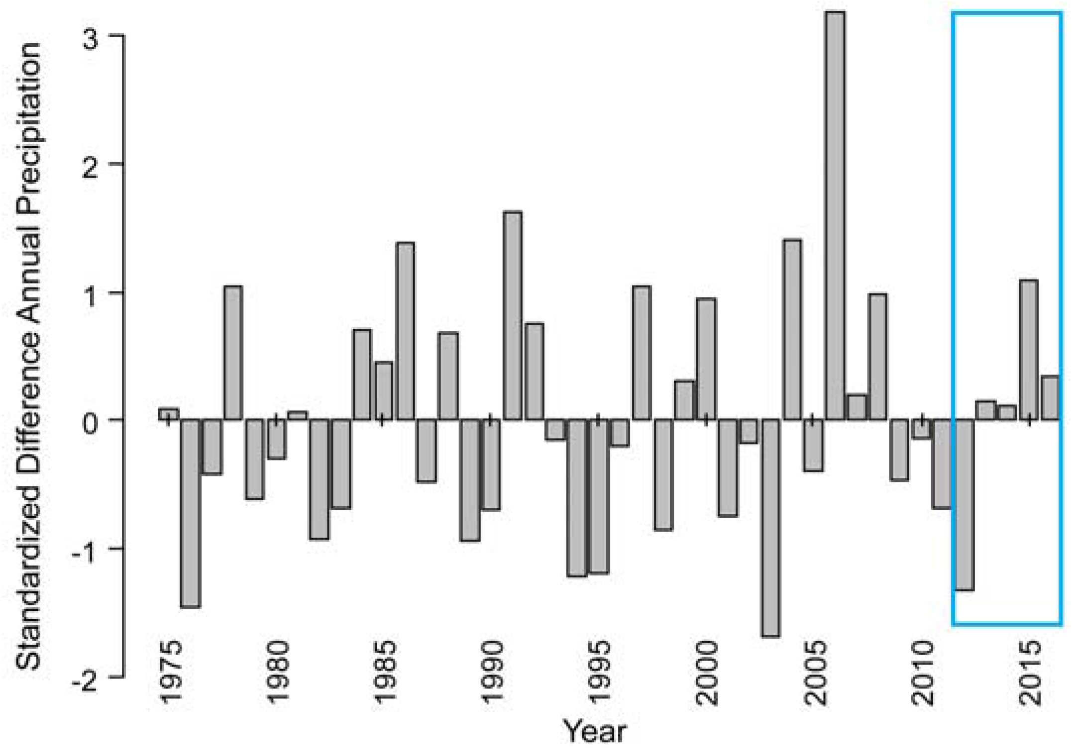
  32. Havstad, K.M.; Huennecke, L.F.; Schlesinger, W.H. Structure and Function of a Chihuahuan Desert Ecosystem. The Jornada Basin Long-Term Ecological Research Site; Oxford University Press: Oxford, UK, 2006; p. 465. [Google Scholar]
  33. Seager, R.; Ting, M.F.; Held, I.; Kushnir, Y.; Lu, J.; Vecchi, G.; Huang, H.P.; Harnik, N.; Leetmaa, A.; Lau, N.C.; et al. Model projections of an imminent transition to a more arid climate in southwestern North America. Science 2007, 316, 1181–1184. [Google Scholar] [CrossRef] [PubMed]
  34. Wainwright, J. Climate and climatological variations in the jornada basin. In Structure and Function of a Chihuahuan Desert Ecosystem. The Jornada Basin Long-Term Ecological Research Site; Havstad, K.M., Huennecke, L.F., Schlesinger, W.H., Eds.; Oxford University Press: Oxford, UK, 2006; pp. 44–80. [Google Scholar]
  35. USDA-NRCS. Ecological Site Information System; National Resource Conservation Service: Lincoln, NE, USA, 2010.
  36. Gibbens, R.P.; McNeely, R.P.; Havstad, K.M.; Beck, R.F.; Nolen, B. Vegetation changes in the Jornada basin from 1858 to 1998. J. Arid Environ. 2005, 61, 651–668. [Google Scholar] [CrossRef]
  37. Browning, D.M.; Duniway, M.C.; Laliberte, A.S.; Rango, A. Hierarchical analysis of vegetation dynamics over 71 years: Soil-rainfall interactions in a Chihuahuan Desert ecosystem. Ecol. Appl. 2012, 22, 909–926. [Google Scholar] [CrossRef] [PubMed]
  38. Eldridge, D.J.; Bowker, M.A.; Maestre, F.T.; Roger, E.; Reynolds, J.F.; Whitford, W.G. Impacts of shrub encroachment on ecosystem structure and functioning: Towards a global synthesis. Ecol. Lett. 2011, 14, 709–722. [Google Scholar] [CrossRef] [PubMed]
  39. Kemp, P.R. Phenological patterns of Chihuahuan Desert plants in relation to timing of water availability. J. Ecol. 1983, 71, 427–436. [Google Scholar] [CrossRef]
  40. Duniway, M.C.; Herrick, J.E.; Monger, H.C. Spatial and temporal variability of plant-available water in calcium carbonate-cemented soils and consequences for arid ecosystem resilience. Oecologia 2010, 163, 215–226. [Google Scholar] [CrossRef] [PubMed]
  41. Gibbens, R.P.; Lenz, J.M. Root systems of some Chihuahuan Desert plants. J. Arid Environ. 2001, 49, 221–263. [Google Scholar] [CrossRef]
  42. Denny, E.G.; Gerst, K.L.; Miller-Rushing, A.J.; Tierney, G.L.; Crimmins, T.M.; Enquist, C.A.F.; Guertin, P.; Rosemartin, A.H.; Schwartz, M.D.; Thomas, K.A.; et al. Standardized phenology monitoring methods to track plant and animal activity for science and resource management applications. Int. J. Biometeorol. 2014, 58, 591–601. [Google Scholar] [CrossRef] [PubMed]
  43. Miller-Rushing, A.J.; Weltzin, J. Phenology as a tool to link ecology and sustainable decision making in a dynamic environment. New Phytol. 2009, 184, 743–745. [Google Scholar] [CrossRef] [PubMed]
  44. Sakamoto, T.; Gitelson, A.A.; Arkebauer, T.J. Modis-based corn grain yield estimation model incorporating crop phenology information. Remote Sens. Environ. 2013, 131, 215–231. [Google Scholar] [CrossRef]
  45. Piao, S.; Tan, J.; Chen, A.; Fu, Y.H.; Ciais, P.; Liu, Q.; Janssens, I.A.; Vicca, S.; Zeng, Z.; Jeong, S.-J.; et al. Leaf onset in the northern hemisphere triggered by daytime temperature. Nat. Commun. 2015, 6. [Google Scholar] [CrossRef] [PubMed]
  46. Gillette, D.; Monger, H.C. Eolian processes on the jornada basin. In Structure and Function of a Chihuahuan Desert Ecosystem. The Jornada Basin Long-Term Ecological Research Site; Havstad, K.M., Huennecke, L.F., Schlesinger, W.H., Eds.; Oxford University Press: Oxford, UK, 2006; pp. 189–210. [Google Scholar]
  47. Keenan, T.F.; Gray, J.; Friedl, M.A.; Toomey, M.; Bohrer, G.; Hollinger, D.Y.; Munger, J.W.; O’Keefe, J.; Schmid, H.P.; SueWing, I.; et al. Net carbon uptake has increased through warming-induced changes in temperate forest phenology. Nat. Clim. Chang. 2014, 4, 598–604. [Google Scholar] [CrossRef]
  48. Jonsson, P.; Eklundh, L. Timesat—A program for analyzing time-series of satellite sensor data. Comput. Geosci. 2004, 30, 833–845. [Google Scholar] [CrossRef]
  49. Gherardi, L.A.; Sala, O.E. Enhanced precipitation variability decreases grass- and increases shrub-productivity. Proc. Natl. Acad. Sci. USA 2015, 112, 12735–12740. [Google Scholar] [CrossRef] [PubMed]
  50. Browning, D.M.; Maynard, J.J.; Karl, J.W.; Peters, D.C. Breaks in modis time series portend vegetation change: Verification using long-term data in an arid grassland ecosystem. Ecol. Appl. 2017, 27, 1677–1693. [Google Scholar] [CrossRef] [PubMed]
  51. Hufkens, K.; Keenan, T.F.; Flanagan, L.B.; Scott, R.L.; Bernacchi, C.J.; Joo, E.; Brunsell, N.A.; Verfaillie, J.; Richardson, A.D. Productivity of North American grasslands is increased under future climate scenarios despite rising aridity. Nat. Clim. Chang. 2016, 6, 710–714. [Google Scholar] [CrossRef]
  52. Munson, S.M.; Long, A.L. Climate drives shifts in grass reproductive phenology across the western USA. New Phytol. 2017, 213, 1945–1955. [Google Scholar] [CrossRef] [PubMed]
  53. Munson, S.M.; Muldavin, E.H.; Belnap, J.; Peters, D.P.C.; Anderson, J.P.; Reiser, M.H.; Gallo, K.; Melgoza-Castillo, A.; Herrick, J.E.; Christiansen, T.A. Regional signatures of plant response to drought and elevated temperature across a desert ecosystem. Ecology 2013, 94, 2030–2041. [Google Scholar] [CrossRef] [PubMed]
  54. Richardson, A.D.; Klosterman, S.; Toomey, M. Near-surface sensor-derived phenology. In Phenology: An Integrative Science; Schwartz, M.D., Ed.; Springer Science+Business Media: Berlin, Germany, 2013; pp. 413–430. [Google Scholar]
  55. Petach, A.R.; Toomey, M.; Aubrecht, D.M.; Richardson, A.D. Monitoring vegetation phenology using an infrared-enabled security camera. Agric. For. Meteorol. 2014, 195, 143–151. [Google Scholar] [CrossRef] [Green Version]
  56. Kao, R.H.; Gibson, C.M.; Gallery, R.E.; Meier, C.L.; Barnett, D.T.; Docherty, K.M.; Blevins, K.K.; Travers, P.D.; Azuaje, E.; Springer, Y.P.; et al. NEON terrestrial field observations: Designing continental-scale, standardized sampling. Ecosphere 2012, 3, 1–17. [Google Scholar] [CrossRef]
  57. Richardson, A.D.; Hufkens, K.; Milliman, T.; Aubrecht, D.M.; Chen, M.; Gray, J.M.; Johnston, M.R.; Keenan, T.F.; Klosterman, S.T.; Kosmala, M.; et al. Tracking Vegetation phenology across diverse north American biomes using phenocam imagery. Scientific Data 2017. submitted. [Google Scholar]
Figure 1. Standardized difference from long-term (1970–2016) mean rainfall on the Jornada Experimental Range (JER). Standardized difference is the individual year value minus long-term average (237.2 mm) divided by the standard deviation (SD 79.6 mm). The five-year study period (2012–2016) is delineated by the blue box.
Remotesensing 09 01071 g001
Figure 2. Fields of view for: Plantcam (A); and Netcam (B). Polygon outlines represent regions of interest (ROIs): black grama (white), mesquite (yellow) and landscape (black). Configuration of two cameras (red stars) relative to focal plants (yellow triangles) and the approximated areal extent of camera fields of view area are depicted as blue polygons (C). The underlying image was acquired from an unmanned aerial system on 23 October 2013.
Remotesensing 09 01071 g002
Figure 3. Framework to compare growing season metrics for grass (black grama, light green) and shrub (mesquite, brown) species from field and Phenocam GCC observations and for landscape greenness (gray) from Phenocam GCC and MODIS NDVI observations for a desert grassland landscape.
Remotesensing 09 01071 g003
Figure 4. (AE): Phenocam GCC for: black grama (A); and mesquite (C) ROIs; and mean field-estimated percent canopy greenness for: black grama (B); and mesquite (D), from 2012 to 2016. Standard deviation of mean canopy greenness is noted by vertical gray lines in (B,D). SOS and EOS are the left and right edges of the gray rectangles in (B,D). SOS in 2012 was estimated from weekly observations of condition that did include intensity metrics until May 2012. Daily precipitation (cm) is depicted (E).
Remotesensing 09 01071 g004
Figure 5. Boxplots representing field-observed and phenocam-derived GCC SOS and EOS dates for: black grama grass (AD); and mesquite shrub (EH) ROIs. Comparisons with significant differences using a paired t-test are noted with an asterisk. In box plots, the middle vertical black line represents the median date and horizontal lines denote the min and max date.
Remotesensing 09 01071 g005
Figure 6. Linear regressions for SOS and EOS seasonal metrics from phenocam GCC for the landscape ROI with MODIS NDVI. SOS and EOS metrics derived from Timesat with four seasonal amplitude thresholds.
Remotesensing 09 01071 g006
Figure 7. Landscape GCC from Plantcam (dotted gray) and Netcam (solid gray) digital cameras with MODIS NDVI (black line) (A). Brown arrows in (A) indicate increases in landscape GCC reflecting mesquite green-up as shown in Figure 4C. Daily precipitation (cm) is depicted (B).
Remotesensing 09 01071 g007
Table 1. Field-observed dates for growing season start (SOS; unfolded leaves) and growing season end (EOS; green leaves =0) for black grama (Bouteloua eriopoda) and mesquite (Prosopis glandulosa) focal plants. Dates are reported as day of year. Observations were collected every seven days using standardized protocols [42]. Values are the mean date for five focal plants with SD in parentheses.
SpeciesYearSOSEOSDuration (# Days)
Black grama201287 (7.7)308 (3.1)221
Black grama2013203 (0.0)325 (3.8)122
Black grama2014127 (34.4)334 (11.5)207
Black grama201589 (0.0)355 (0.0)266
Black grama201666 (2.7)306 (0.0)240
Mesquite2012114 (4.9)324 (0.0)210
Mesquite2013108 (3.8)335 (3.1)227
Mesquite2014101 (7.8)330 (0.0)229
Mesquite2015109 (15.4)340 (7.7)231
Mesquite2016114 (3.8)354 (3.1)240
Table 2. Summary of root mean square error (RMSE) as the absolute difference in the number of days for comparisons of field-observed growing season start (SOS) and end (EOS) dates with those derived from phenocam GCC using the Timesat with four percent seasonal amplitude thresholds.
TargetMetricThresholdRMSE
Black gramaSOS10105.4
Black gramaSOS15107.1
Black gramaSOS20107.9
Black gramaSOS25109.2
Black gramaEOS1023.9
Black gramaEOS1522.6
Black gramaEOS2028.9
Black gramaEOS2532.8
MesquiteSOS108.6
MesquiteSOS1510.6
MesquiteSOS2012.9
MesquiteSOS2513.6
MesquiteEOS1016.3
MesquiteEOS159.9
MesquiteEOS208.3
MesquiteEOS258.2
Table 3. Summary of root mean square error (RMSE) as the absolute difference in the number of days for comparisons of phenocam landscape GCC with SOS and EOS dates derived from 250-m NDVI. SOS and EOS dates were derived using Timesat with four seasonal amplitude thresholds.
Metric MethodMetricThresholdRMSE
TimesatSOS1063.5
TimesatSOS1547.3
TimesatSOS2057.8
TimesatSOS2536.8
TimesatEOS1044.1
TimesatEOS1546.8
TimesatEOS2039.6
TimesatEOS2534.7

