Agricultural Soil Spectral Response and Properties Assessment: Effects of Measurement Protocol and Data Mining Technique

Abstract

Soil spectroscopy has shown to be a fast, cost-effective, environmentally friendly, non-destructive, reproducible and repeatable analytical technique. Soil components, as well as types of instruments, protocols, sampling methods, sample preparation, spectral acquisition techniques and analytical algorithms have a combined influence on the final performance. Therefore, it is important to characterize these differences and to introduce an effective approach in order to minimize the technical factors that alter reflectance spectra and consequent prediction. To quantify this alteration, a joint project between Czech University of Life Sciences Prague (CULS) and Tel-Aviv University (TAU) was conducted to estimate Cox, pH-H₂O, pH-KCl and selected forms of Fe and Mn. Two different soil spectral measurement protocols and two data mining techniques were used to examine seventy-eight soil samples from five agricultural areas in different parts of the Czech Republic. Spectral measurements at both laboratories were made using different ASD spectroradiometers. The CULS protocol was based on employing a contact probe (CP) spectral measurement scheme, while the TAU protocol was carried out using a CP measurement method, accompanied with the internal soil standard (ISS) procedure. Two spectral datasets, acquired from different protocols, were both analyzed using partial least square regression (PLSR) technique as well as the PARACUDA II^®, a new data mining engine for optimizing PLSR models. The results showed that spectra based on the CULS setup (non-ISS) demonstrated significantly higher albedo intensity and reflectance values relative to the TAU setup with ISS. However, the majority of statistics using the TAU protocol was not noticeably better than the CULS spectra. The paper also highlighted that under both measurement protocols, the PARACUDA II^® engine proved to be a powerful tool for providing better results than PLSR. Such initiative is not only a way to unlock current limitations of soil spectroscopy, but also offers considerable efficiency and cost- and time-saving possibilities, which lead to further improvements in prediction performance of spectral models.

1. Introduction

Soil reflectance analysis in the visible-near infrared-short wave infrared (VIS-NIR-SWIR) region has become a well-recognized, rapid and reproducible analytical method that has been used for non-destructive and low-cost soil analyses [1]. It differentiates materials based on their reflectance in the wavelength range from 400–2500 and can be used to encode information on the inherent composition of soil and determine a wide range of soil parameters in different platforms (in the laboratory, in the field using sampling, on-the-go using sensors embedded on a tractor, as well as airborne measurements) [2,3,4].

Although the technique is mainly used under controlled laboratory conditions, with the rise in available portable spectrometers, its application in situ [5], as well as from the air- and space-borne sensors, is growing [6,7]. Under in-situ measurement conditions, additional challenges associated with the variation of soil-to-sensor distance affect the accuracy of the measurement [8,9]. In addition, a wide range of soil spectral measurements are being gathered around the globe, which return different results as they have been collected with different protocols, sampling techniques, sample preparation, instrument specifications, spectral acquisition and analytical algorithms, and can severely affect the prediction performance of spectroscopic models and outputs [4,10,11]. For instance, differences in water content of air-dried samples (depending on the laboratory protocol), due to fluctuations in relative humidity of the ambient air in the laboratory, affect the spectral shape and peaks, especially around 1415 and 1915 nm [12,13]. According to Soriano-Disla et al. [4], spectral reflectance is also affected by the grinding of soil, which can generate important differences of accuracy in the prediction models due to the variation of particle sizes, the same is true for sieving. Suitable data preprocessing, calibration and validation strategies, which frequently differ for users and operators, to calibrate soil prediction models, influence the final model too. For example, Gholizadeh et al. [14] indicated that the 1st derivative preprocessing method gave the best prediction of heavy metals in the Czech Republic mining areas, in comparison to 2nd derivative, multiplicative scatter correction (MSC), standard normal variate (SNV) and continuum removal (CR). Viscarra Rossel and Behrens [15] and Araujo et al. [16] applied partial least square regression (PLSR), boosted regression trees (BRT) and support vector machine regression (SVMR) methods for the prediction of clay; SVMR offered the most successful prediction model due to its ability to solve the multivariate calibration problems and to reduce problems with heterogeneity and non-linearity. However, in a study by Gholizadeh et al. [17], the memory based learning (MBL) technique outperformed PLSR, BRT and SVMR in soil texture prediction, which can be attributed to the selection of more appropriate neighbours to calibrate local models, as well as the inclusion of more suitable neighbours in each local model as a source of additional predictor variables [18]. Factors such as different populations, different partitions of the population for the analyses and environmental condition may also cause variation.

To overcome these difficulties that block any attempt for reliability and comparability of results [19], some solutions were suggested by researchers; these included the selection of proper instrumentation, standards and protocol development [20], improved spectra filtering and preprocessing [21], better control of ambient conditions [8] and the appropriate selection of multivariate statistical analysis [15,22]. These approaches can significantly reduce differences between spectral measurements of the same samples by different operators in different laboratories. Since calibration and management represent a large part of costs and efforts in the use of spectroscopy techniques to standardization and more suitable methods are strongly needed, the current study compares two measurement protocols and two modelling techniques using the exact same soil population. To this end, we compared the measurement protocols in terms of their effects on samples spectral responses: The first is the protocol developed at Czech University of Life Sciences Prague (CULS) and the second is the protocol developed by Ben-Dor et al. [20] at Tel-Aviv University (TAU). The other experiment was to use the common PLSR technique on spectra collected using both protocols and compare it to the all-possibilities approach using the PARACUDA II^® engine, a new data mining and model optimizing approach, to extract proxy models of some soil attributes, namely, oxidizable carbon (Cox), pH-H₂O, pH-KCl, crystalline Fe and Mn (Fe-d and Mn-d) and amorphous Fe and Mn (Fe-ox and Mn-ox). The PARACUDA II^® engine has been designed to utilize parallel and automatic processing in order to build and process hundreds of diverse models in order to prevent errors or biases caused by a human operator in the loop, when taking the model setting decision. PARACUDA II^® also enables us to check all of the possible preprocessing combinations along with different statistical methods automatically and rapidly, which in reality are almost impossible for a single user to perform in a reasonable amount of time. This study involved a comprehensive collaboration between CULS and TAU.

2. Materials and Methods

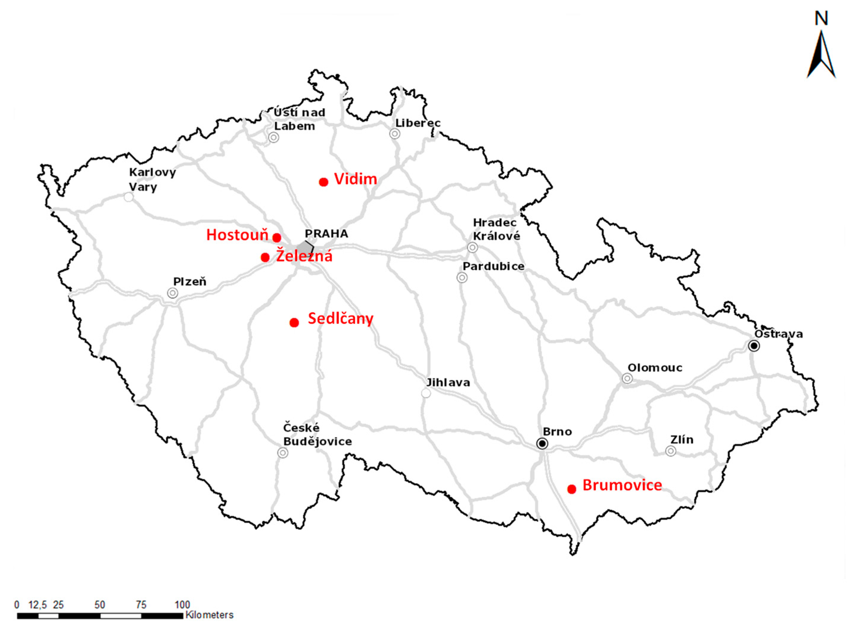
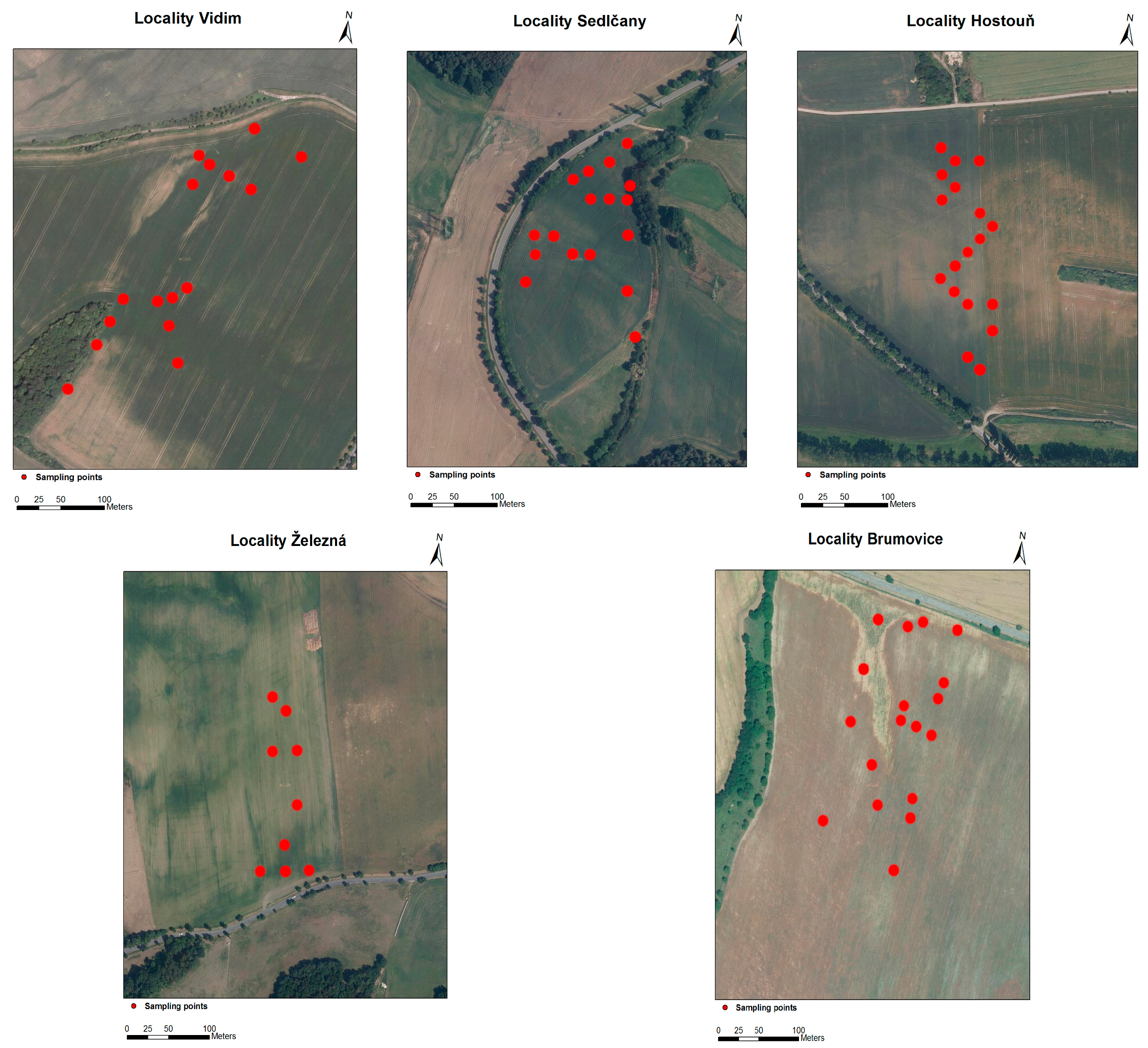
2.1. Study Area

Five agricultural areas from different parts of the Czech Republic were selected (Figure 1): Vidim (50°46′N; 14°51′E, area 8 ha, altitude 315–323 m above sea level (a.s.l.), average annual temperature 7–8 °C, average precipitation 550–650 mm), Sedlčany (49°68′N; 14°42′E, area 4 ha, altitude 375–387 m a.s.l., average annual temperature 7–8 °C, average precipitation 550–650 mm), Hostouň (50°12′N; 14°21′E, area 3 ha, altitude 335–358 m a.s.l., average annual temperature 8–9 °C, average precipitation <500 mm), Železná (50°00′N; 14°09′E, area 3 ha, altitude 395–419 m a.s.l., average annual temperature 7–8.5 °C, average precipitation 450–550 mm) and Brumovice (48°96′N; 16°88′E, area 6 ha, altitude 187–227 m a.s.l., average annual temperature 9–10 °C, average precipitation 500–600 mm). According to the World reference base (WRB) for soil resources in 2014, the original soil type in Brumovice was Haplic Chernozem on loess, which due to erosion changed into Regosol (steep parts) and Colluvial soil (base slope and the tributary valley). A similar process can be observed at the four other locations Vidim, Sedlčany, Hostouň and Železná, where the original soil types were Haplic Luvisol on loess, Haplic Cambisol on gneiss, Calcaric Leptosol on marlite and Haplic Cambisol on shales, respectively.

2.2. Soil Sampling and Analysis

78 soil samples were taken from the topsoil (0–20 cm) within a regular grid covering the studied areas: 16 samples on Vidim, 17 samples on Sedlčany, 18 samples on Hostouň, nine samples on Železná and 18 samples on Brumovice (Figure 2). Regarding field size and the chosen sampling algorithm [23,24], the selected sample size had sufficient coverage of the predictor space and it was a suitable indicator of the population in which the models were applied.

All of the samples were air-dried and sieved to <2 mm and then stored in plastic containers. The basic chemical and physical soil properties were obtained using standard laboratory procedures under a constant laboratory temperature of 20 °C. The Cox was measured using the dichromate redox titration method [25]. Wet oxidation (K₂Cr₂O₇) of the samples was followed by a potentiometric titration with ferrous ammonium sulphate. The soil pH was measured using a 1:5 (w/v) ratio of soil and water (pH-H₂O) and 1 M potassium chloride (pH-KCl) solutions based on International Organization of Standardization (ISO 10390:1994) using an inoLab Level 1 pH-meter. The content of Fe and Mn forms was determined in all of the samples by simple extraction methods. While the extracted forms of Fe can be classified as being labile, amorphous and crystalline [26,27,28], in the case of Mn, this designation is rather more ambiguous [29]. The amount of crystalline forms (Fe-d, Mn-d) was determined by extraction with a dithionite citrate (DC) solution [30,31] at a ratio of 0.5:25 (w/v) [28]. According to Guest et al. [29], extraction with dithionite citrate bicarbonate (DCB) [32] gives similar results as with DC [33], and determines the finely crystalline phases of Mn²⁺ and Mn³⁺ with quadrivalent Mn most likely not being extracted. In the reducing conditions, Mn is also extracted from the structure of Fe-oxides. In contrast, bivalent and trivalent Mn occurring in the structure of clay minerals and in primary soil minerals are not extracted by DCB or DC. The proportion of amorphous forms and organic complexes (Fe-ox, Mn-ox) was determined with ammonium oxalate. The extraction was carried out according to McKeague and Day [30] and Courchesne and Turmel [28] with 0.2 M of ammonium oxalate at pH 3 at a ratio of 0.25:10 (w/v). The final concentrations of Fe and Mn were subsequently measured by ICP-OES with an iCAP 6500 Radial ICP Emission spectrometer (Thermo Fisher Scientific, Waltham, MA, USA) under standard analytical conditions.

2.3. Reflectance Measurements

After soil chemical analysis and spectral measurements at CULS, the samples were sent to TAU and spectral analysis was performed at this institution under different spectral measurement protocols. In both laboratories, spectral reflectance was deliberated across the 350–2500 nm wavelength range using an ASD FieldSpec III Pro FR spectroradiometer (ASD Inc., Denver, Boulder, CO, USA). The spectral resolution of the spectroradiometer was 2 nm for the region 350–1050 nm and 10 nm for the region 1050–2500 nm (495 individual spectral bands were calculated). The radiometer bandwidth from 350–1000 nm was 1.4 nm, while it was 2 nm from 1000–2500 nm.

2.3.1. CULS Protocol

A high intensity contact probe (CP) was chosen for the spectral measurement at CULS. The instrument ran for ~30 min to warm up the spectrometer and lamp. Soil samples were placed in 9 cm diameter petri dishes, forming a 2 cm layer of soil. This was to avoid beam reflectance from the bottom of the dish due to down-welling solar and sky radiation penetrating into the soil at approximately 1/2 wavelength [34], which could have an unwanted effect of modifying the soil spectra. Samples were levelled off using a stainless steel blade to guarantee a flat surface flush with the top of the petri dish, as a smooth soil surface ensures maximum light reflection and a high signal-to-noise ratio [35]. All of the spectral readings were measured in the center of the samples (three replications each) in a dark room to avoid interference from stray light. The spectroradiometer was optimized using a white Spectralon™ (Lab-sphere, North Sutton, NH, USA) prior to the first scan and after every six measurements [36]. For each soil measurement, 30 spectra were averaged to improve signal-to-noise ratio. Noisy portions between 350–400 nm and 2450–2500 nm were removed, leaving spectra in the range from 400–2450 nm for our analysis.

2.3.2. TAU Protocol

The spectra measurement at TAU was carried out using a high intensity CP according to the Commonwealth Scientific and Industrial Research Organization (CSIRO) protocol [20] and internal soil standard (ISS) procedure. The ISS idea is based on the fact that the non-systematic effects, such as random noise, uncertain effects and instabilities are minimized by the protocol used in the professional laboratory, while the different systematic effects between protocols are corrected for using the alignment factor generated from a well-known and agreed standard’s reading [23]. The introduced ISS sample by Ben-Dor et al. [20] were homogeneous sand dunes along the coastline of Lucky Bay (33°59′S; 122°13′E) in southwestern Australia, which were found to be excellent for the ISS concept.

The protocol’s arrangement requires 60 min of warming up the spectrometer and 30 min for the lamps. The samples were prepared by pressing the soil surface against a glass surface and bringing the bare samples to the CP by a stable elevator while the CP was held firmly in place. The sample preparation was done using a large sample holder with surface preparation consisting of a flat sheet of glass being used to apply pressure and flatten the surface. Three replications were used for each sample, which originated from the same sample holder and was re-prepared after mixing it again for measurement. After each measurement, a check was performed to determine if the white reference was observed to have returned to 100%. If necessary, the white reference was retaken to set it back to 100%. The ISS was measured using the same configuration before and after each five samples were inspected for variation. The correction factor was calculated by dividing the ISS sample spectra measured before and after the five samples in the motherhood ISS spectra measured at CSIRO. This factor was then applied to five soil samples in order to standardize their spectra.

2.4. Spectral Modelling

Spectral modelling of the selected soil attributes was performed using different techniques to explore and compare the capability of the PLSR method, the most common algorithm for VIS-NIR-SWIR spectra calibration of soil properties, and the PARACUDA II^®, the all-possibilities approach data mining engine.

2.4.1. PLSR Modelling

At both institutions, the spectral modelling first was done by employing a PLSR model under an original raw spectral dataset, and two different datasets that were yielded after preprocessing techniques including 1st and 2nd derivatives. The validation technique was 10-fold cross-validation. A brief summary of the algorithm is as follows:

The PLSR, which has turned into a popular algorithm in chemometrics, decreases the data, noise and calculation time with minor loss of the information contained in the original variables [37] and its arithmetic can be found in Wold et al. [38]. It is strongly related to principal component regression (PCR), in that both methods use statistical rotations to defeat the problem of high dimensionality and multicollinearity [39,40]. They both compress the data before completing the regression. The difference is that PLSR algorithm combines the compression and regression steps, and it selects successive orthogonal factors that maximize the covariance between predictor and response variables [15,40,41,42]. By fitting a PLSR model, one expects to discover a few PLSR factors that clarify most of the variation in both predictors and responses [43]. It can be said that in PLSR, an essential step is the selection of the optimal number of latent variables (nLV) in the calibration model to avoid under-fitting and over-fitting of data that would generate models with poor prediction potential [44,45].

2.4.2. PARACUDA II^® Modelling

Spectral modelling of the provided soil attributes at CULS and TAU was then performed using the PARACUDA II^®, a new data mining and model optimizing approach, which has been developed at the remote sensing laboratory of TAU by Carmon and Ben-Dor [46]. This is a sophisticated program based on the all-possibilities-approach (APA) concept, a conditional Latin hypercube sampling (cLHs) algorithm and parallel programming to evaluate all of the potential combinations of manipulations (preprocessing) to the original reflectance and chemical data prior to model development. PARACUDA II^® has four main steps, each with an exact purpose in the modelling procedure, namely (i) outlier detection and elimination; (ii) preprocessing and transformations; (iii) model development and validation; and (iv) population analysis and best model selection. A schematic of the PARACUDA II^® processing framework can be seen in Figure 3.

At the first step, the outlier detection and elimination module for the spectral and the chemical datasets, the chemical values for the specific task is transformed into z-scores and a pre-configured threshold value to remove outliers is employed. The chemical values above or below ±2, which are in the 2.5% out range of a normal distribution, are excluded from the population (in this study 2–5 samples, depending on the property). For spectral data outlier detection, a principle component analysis (PCA) calculation is used to derive the first two factors. Then, samples beyond a 95% confidence ellipse on the two factors are detected and eliminated from the population. The algorithm, cLHs, is used to divide the data into calibration and validation groups, which characterize the most variability of the data within the two groups by data sub-setting based on a Gaussian distribution. The next step is preprocessing and transformations in which the chemical values are transformed using a Box-Cox algorithm to achieve a more normal distribution. However, the spectra are subjected to a sequence of preprocessing calculation based on APA using eight different spectral preprocessing algorithms, namely moving average, 1st and 2nd derivatives, absorbance transformation, CR, SNV, MSC and final smoothing, in all mathematically possible combinations, resulting with up to 120 preprocessing sequences. Then, the correlation between every spectral combination at each wavelength and the modeled chemical values is evaluated, the combination with the highest correlation chosen for further steps. The output of this sequence is a set of different transformation values for every wavelength, which shows the highest covariation with the modeled properties. Instead of relying on a single or arbitrarily selected sequence for the whole wavelength region, we actually extracted all of the manipulations for the spectral dataset. The final product of this step is a new dataset containing the values of different and optimal preprocessing techniques for every wavelength separately. After the data transformation, preprocessing and grouping, the calibration set is used for finding the best preprocessing sequence, the optimal nLV and calculate the prediction model. To find the best per-wavelength combination, the coefficient of determination (R²) between each preprocessing combination at each wavelength to the chemical values is calculated. The optimal nLV is computed by determining the percentage of variance (PCTVAR) of the modeled values for models with between 5 and 15 factors. Finally, the main PLSR model is developed and a model on the per-wavelength preprocessed data and the transformed chemical values with the optimal nLV and on the calibration group is created. During the third step, model development and validation, a PLSR model is developed on transformed and preprocessed data without overfitting. The sequence starting from the sampling routine and finishing in the prediction model evaluation is repeated 512 times. To test the derived models, the validation group samples are preprocessed with the same routine as the calibration samples. The model is applied on the samples and the predicted values are transformed back from Box-Cox values to original chemical values. After completion of the iterative procedure, 512 unique PLSR models with their performance statistics are available. For step four, population analysis and best model selection, a R² per wavelength for the preprocessed data, as well as the weighted average beta coefficients of the best model of the 512 iterations are performed. These spectra are useful for understanding the important spectral ranges of specific chemical attributes and for providing further observation of the results. PARACUDA II^® outputs are two files, the first file is the summary report of the calibration group, validation group, cross-validation and the two spectral assignment spectra in Excel format, providing measured and predicted values for each attribute and the second file is an applicable model in Matlab format, ready to be applied on new spectral data. The second file is useful for either further validation or practical purposes and can be applied on both point spectral data or on a hyperspectral image directly from the PARACUDA II^® interface.

2.5. Assessment Statistics

The R² and the root mean square error (RMSE) have been reported as standard methods for validation of the prediction models [47]. Therefore, to compare the ability of different established calibration methods, the R² and the RMSE of cross-validation from the PLSR, as well as the R² and the RMSE from the test-set for PARACUDA II^® at both institutions, were considered. R² shows the percentage of the variance in the y variable that is calculated by the x variables, and RMSE indicates the prediction error. Generally, the best prediction model is shown by the largest R² and the smallest RMSE [47].

3. Results and Discussion

3.1. Soil Descriptive Statistics

Descriptive statistical results of soil parameters are summarized in

Table 1. Descriptive statistics of soil properties in the studied sample sets.

Characteristic	Cox	pH-H2O	pH-KCl	Fe-d	Fe-ox	Mn-d	Mn-ox
	(%)			mg kg−1
Min	0.6	5.3	4.5	4360	620	122	140
Max	3.0	8.6	7.6	19,784	4280	573	478
Mean	1.5	7.3	6.6	9151	1775	350	260
SD	0.5	0.9	1.0	3112	891	89	88
CV (%)	33	12	15	34	50	25	34

. The studied samples represented a narrow range of pH-H₂O and pH-KCl (ranging from 5.3–8.6 and 4.5–7.6, respectively); however, they varied widely in the case of Fe. The comparison of coefficients of variation (CV) of different parameters showed that among all of the parameters, distribution of pH-H₂O was more homogeneous, it had the lowest CV and varied less when compared to other considered attributes (12%). In contrast, Fe-ox had high CV (50%), underlining the varied and diverse origin of the samples.

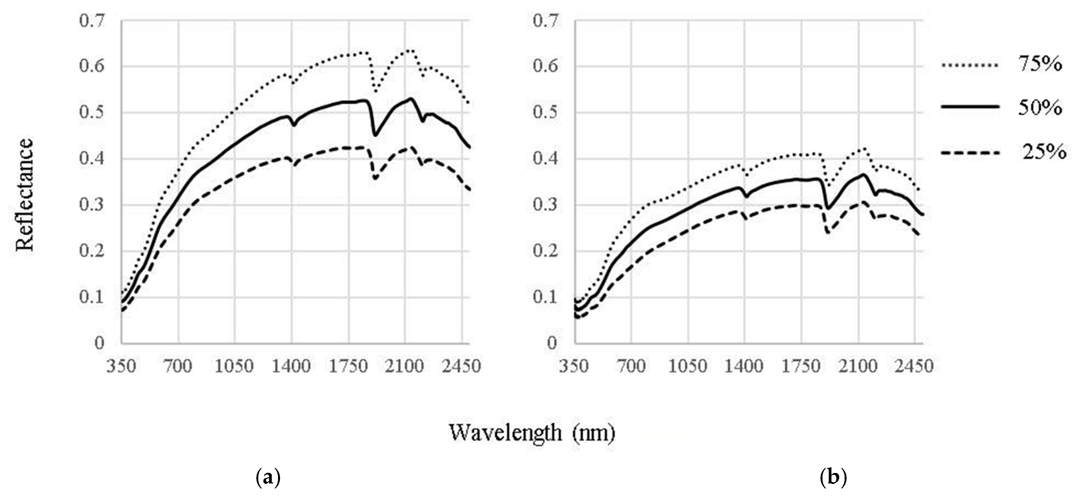
3.2. Soil Spectral Reflectance Pattern

The spectral responses of soil samples, measured at CULS and TAU, are presented in Figure 4. Both spectra had a similar general form with reflectance increasing with increasing of wavelength in the VIS range. A broad region within which there were sharp absorption bands in the infrared range was also obvious at both institutions measured spectra. Soil reflectance, like other soil properties, varies continuously and the resulting spectra represent complex compositional mixtures of soil materials from diverse origins that are also affected by their environments. It is clear that VIS-NIR-SWIR spectra contain useful information that can be used to derive estimates of soil properties. For example, absorption features in the VIS-NIR wavelength (400–1000 nm) are characteristics of the presence of soil carbon and iron oxide [34,35,48,49,50], and those in the SWIR (1000–2500 nm) are from water, clay minerals and organic matter [16,51]. The important spectra absorption features through the use of some data mining algorithms have been studied by Viscarra Rossel and Behrens [15] and Gholizadeh et al. [17].

Figure 5 demonstrates the spectra of soil samples based on their median, 1st and 3rd quartiles, as measured by both institutions protocols. It can be clearly seen that spectral shape and position at both CULS and TAU protocols did not show any noticeable difference, though spectra based on the CULS setup demonstrated apparently higher albedo intensity and reflectance values relative to the TAU setup reflectance. This is partly due to the fact that the measurement conditions (different sample preparation, different environments, different white references, different bulbs and illumination situation) for the TAU protocol were different to those at CULS, and more important due to applying ISS correction factors at TAU, which decreased the spectral variation and was able to correct the TAU spectra. According to Pimstein et al. [23], the albedo intensity may refer to an offsetting of the spectral baseline. They also mentioned the higher reflectance, suggesting that the differences in relative humidity during the measurements in different laboratories might be affecting the spectral response.

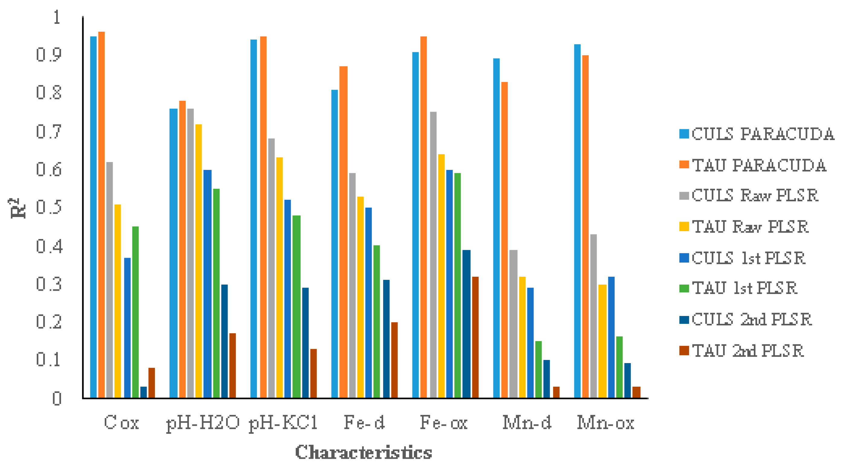
3.3. Comparison of Predictions Using Different Protocols and Algorithms

3.3.1. PLSR on CULS and TAU Spectral Datasets

Table 2. PLSR performance for CULS and TAU spectral datasets.

Attribute	Raw Spectra				1st Derivative				2nd Derivative
	CULS		TAU		CULS		TAU		CULS		TAU
	R2	RMSE	R2	RMSE	R2	RMSE	R2	RMSE	R2	RMSE	R2	RMSE
Cox	0.62	0.32	0.51	0.35	0.37	0.46	0.45	0.38	0.03	0.58	0.08	0.48
pH-H2O	0.76	0.46	0.72	0.50	0.60	0.64	0.59	0.63	0.30	0.84	0.20	0.85
pH-KCl	0.68	0.55	0.63	0.58	0.52	0.73	0.48	0.69	0.29	0.88	0.13	0.89
Fe-d	0.59	2000	0.53	2123	0.50	2220	0.40	2451	0.31	2600	0.17	2785
Fe-ox	0.75	453.36	0.64	533.70	0.60	599.84	0.55	598.60	0.39	701.08	0.32	725.23
Mn-d	0.39	69.83	0.32	73.67	0.29	75.89	0.15	82.67	0.10	84.71	0.03	87.51
Mn-ox	0.43	66.51	0.30	74.13	0.32	72.91	0.16	81.45	0.09	84.04	0.03	86.53

provides results of the analysis using PLSR on three spectral datasets of CULS and TAU: original raw spectral data, 1st derivative and 2nd derivative.

In the multivariate calibration, raw spectra provided the best results in comparison to the 1st and 2nd derivatives at both institutions (R² values 0.39–0.76 and 0.30–0.72 at CULS and TAU, respectively). When compared to CULS, TAU protocol in most of statistics gave lower R² and higher RMSE, in spite of employing ISS. Pimstein et al. [23] also noticed the same pattern in their study and mentioned that ISS can bring good results if a standard protocol is used in different laboratories. The most consistent estimates were commonly gained for pH-H₂O and Fe-ox in all three datasets at both CULS and TAU. Good and excellent R² (R² > 0.81 and R² > 0.90, respectively) [52] were not obtained for any of the studied elements ad any of protocols. Inadequate models with poor accuracy (R² < 0.50 and high RMSE) were obtained for Mn-d and Mn-ox in raw spectral data and 1st derivative. 2nd derivative provided poor and unsatisfactory accuracy for all of the treated attributes in both of the laboratories.

3.3.2. PARACUDA II^® on CULS and TAU Spectral Datasets

The PARACUDA II^® results on both the CULS and TAU spectral datasets are given in

Table 3. PARACUDA II^® performance for CULS and TAU spectral datasets.

Attribute	CULS		TAU
	R2	RMSE	R2	RMSE
Cox	0.95	0.09	0.96	0.08
pH-H2O	0.76	0.25	0.78	0.25
pH-KCl	0.94	0.06	0.95	0.05
Fe-d	0.81	0.27	0.87	0.24
Fe-ox	0.91	5.85	0.95	3.65
Mn-d	0.89	39.99	0.83	34.98
Mn-ox	0.93	0.24	0.90	0.36

. The best results of 512 models and the performances of R² and RMSE can be seen. All of the statistics are for maximum R² values of 512 individual model iterations.

Summarizing the results of Table 3, it can be seen that the best predictability from PARACUDA II^® was obtained for Cox (R² = 0.95, RMSE = 0.09; R² = 0.96, RMSE = 0.08), followed by pH-KCl (R² = 0.94, RMSE = 0.06; R = 0.95, RMSE = 0.05) in CULS and TAU measurements, respectively. Moreover, for all of the parameters except Mn, the TAU spectral dataset achieved higher results (but not significantly) than the CULS dataset. The 512 different linear models for the range of soil properties would not be easy to run without the automatic and parallel processing abilities that the PARACUDA II^® offers.

A comparison of R² using different algorithms on different datasets has been summarized in Figure 6. It indicates that a noticeable improvement of both protocols data performances by using PARACUDA II^® was achieved. Accordingly, the PARACUDA II^® provided excellent models, even to those attributes that did not show any model by traditional PLSR. Mn-d and Mn-ox, which provided poor accuracy (R² < 0.50 and high RMSE) using PLSR, showed a quite notable improvement, when PARACUDA II^® was employed. This is mainly because of the capability of PARACUDA II^® to check all the available options and prepare the hidden models, which cannot be depicted by PLSR. As the CULS measurements were acquired under a very accurate and stable procedure (CULS protocol), it is most likely that the non-systematic effects (e.g., random noise, uncertain effects and instabilities) were minimized, hence the PARACUDA II^® could yield very high accuracy as the TAU-ISS protocol provided.

All to all, despite the important influence of ISS on spectra correction and variation reduction, as well as its positive and apparent effect on soil samples spectral responses, the final enhancement of TAU protocol with ISS on statistics was not noticeably better than the non-ISS spectra (the CULS results). Although, it has been demonstrated that ISS is extremely beneficial when combining Soil Spectral Libraries (SSLs) measured with different protocols (users, instrumentation, environment, white reference condition, etc.) [20,23] and may also be useable for instruments’ cross-validation process [53,54]. Accordingly, the PARACUDA II^® data mining engine proved to be a powerful tool for achieving higher results than the regular schemes such as PLSR, which was employed in this study. This can be related to its capability for automatic parallel examination of many data manipulations, as well as generating many partitions of the calibration-validation groups. It also excels in the automatic procedure it provides, which enables searching for the best available model, something that cannot be obtained by a skilled person in a reasonable amount of time.

4. Summary and Conclusions

The results of the study showed that ISS aligned the systematic changes of the TAU protocol to make it more stable; however, the analytical results from the TAU protocol with ISS did not show noticeably higher enhancement than the CULS (non-ISS) outputs. It seems that keeping a protocol (no matter what the protocol is) constant, reduces the efficiency of ISS, as the non-systematic effects are minimal. Although, using ISS is highly recommended for fine-tuning small systematic effects in a given protocol in general and between protocols in particular. In terms of data mining techniques, PARACUDA II^® as a new data mining and model optimizing approach, obviously provided better results and proved to be a powerful and reliable tool in achieving the best prediction model, rather than PLSR as a conventional data mining algorithm; however, PARACUDA II^® is also a PLSR model, but it uses a covariate optimization routine that selects the best preprocessing steps for a given response variable. Based on the promising results of the PARACUDA II^® performance, implementation of further studies with other data mining and machine learning algorithms over different geographic scales is highly advocated in order to check the PARACUDA II^® robustness and stability. In conclusion, adherence to a consistent protocol and a reliable data mining technique will improve the accuracy and the comparability of results, which is necessary for the entire soil community.

References

1. Reeves, J.B., III. Near-versus Mid-Infrared diffuse reflectance spectroscopy for soil analysis emphasizing carbon and laboratory versus on-site analysis: Where are we and what needs to be done? Geoderma 2010, 158, 3–14. [Google Scholar] [CrossRef]
2. Ben-Dor, E.; Patkin, K.; Banin, A.; Karnieli, A. Mapping of several soil properties using DAIS-7915 hyperspectral scanner data- A case study over clayey soils in Israel. Int. J. Remote Sens. 2002, 23, 1043–1062. [Google Scholar] [CrossRef]
3. Gholizadeh, A.; Boruvka, L.; Saberioon, M.M.; Vasat, R. Visible, near-infrared, and mid-infrared spectroscopy applications for soil assessment with emphasis on soil organic matter content and quality: State-of-the-art and key issues. Appl. Spectrosc. 2013, 67, 1349–1362. [Google Scholar] [CrossRef] [PubMed]
4. Soriano-Disla, J.M.; Janik, L.J.; Viscarra Rossel, R.A.; MacDonald, L.M.; McLaughlin, M.J. The performance of visible, near-, and mid-infrared reflectance spectroscopy for prediction of soil physical, chemical, and biological properties. Appl. Spectrosc. Rev. 2014, 49, 139–186. [Google Scholar] [CrossRef]
5. Viscarra Rossel, R.A.; Cattle, S.R.; Ortega, A.; Fouad, Y. In situ measurements of soil colour, mineral composition and clay content by vis-NIR spectroscopy. Geoderma 2009, 150, 253–266. [Google Scholar] [CrossRef]
6. Ben-Dor, E.; Chabrillat, S.; Dematte, J.A.M.; Taylor, G.; Hill, J.; Whiting, M.; Sommer, S. Using imaging spectroscopy to study soil properties. Remote Sens. Environ. 2009, 113, S38–S55. [Google Scholar] [CrossRef]
7. Cecillon, L.; Barthes, B.; Gomez, C.; Ertlen, D.; Genot, V.; Hedde, M.; Stevens, A.; Brun, J. Assessment and monitoring of soil quality using near-infrared reflectance spectroscopy (NIRS). Eur. J. Soil Sci. 2009, 60, 770–784. [Google Scholar] [CrossRef]
8. Mouazen, A.M.; Maleki, M.R.; de Baerdemaeker, J.; Ramon, H. On-line measurement of some selected soil properties using a VIS-NIR sensor. Soil Tillage Res. 2007, 93, 13–27. [Google Scholar] [CrossRef]
9. Waiser, T.H.; Morgan, C.L.S.; Brown, D.J.; Hallmark, C.T. In situ characterization of soil clay content with visible near-infrared diffuse reflectance spectroscopy. Soil Sci. Soc. Am. J. 2007, 71, 389–396. [Google Scholar] [CrossRef]
10. Viscarra Rossel, R. The soil spectroscopy group and the development of a global soil spectral library. NIR News 2009, 20, 14–15. [Google Scholar] [CrossRef]
11. Brown, D.J.; Bricklemyer, R.S.; Miller, P.R. Validation requirements for diffuse reflectance soil characterization models with a case study of VNIR soil C prediction in Montana. Geoderma 2005, 129, 251–267. [Google Scholar] [CrossRef]
12. Whiting, M.L.; Li, L.; Ustin, S.L. Predicting water content using Gaussian model on soil spectra. Remote Sens. Environ. 2004, 89, 535–552. [Google Scholar] [CrossRef]
13. Nocita, M.; Stevens, A.; Noon, C.; van Wesemael, B. Prediction of soil organic carbon for different levels of soil moisture using Vis-NIR spectroscopy. Geoderma 2012, 199, 37–42. [Google Scholar] [CrossRef]
14. Gholizadeh, A.; Boruvka, L.; Vasat, R.; Saberioon, M.M. Comparing different data preprocessing methods for monitoring soil heavy metals based on soil spectral features. Soil Water Res. 2015, 10, 218–227. [Google Scholar] [CrossRef]
15. Viscarra Rossel, R.A.; Behrens, T. Using data mining to model and interpret soil diffuse reflectance spectra. Geoderma 2010, 158, 46–54. [Google Scholar] [CrossRef]
16. Araujo, S.R.; Wetterlind, J.; Dematte, J.A.M.; Stenberg, B. Improving the prediction performance of a large tropical vis-NIR spectroscopic soil library from Brazil by clustering into smaller subsets or use of data mining calibration techniques. Eur. J. Soil Sci. 2014, 65, 718–729. [Google Scholar] [CrossRef]
17. Gholizadeh, A.; Saberioon, M.M.; Boruvka, L.; Vasat, R. A memory-based learning approach as compared to other data mining algorithms for the prediction of soil texture using diffuse reflectance spectra. Remote Sens. 2016, 8, 341. [Google Scholar] [CrossRef]
18. Ramirez-Lopez, L.; Behrens, T.; Schmidt, K.; Stevens, A.; Dematte, J.A.M.; Scholten, T. The spectrum-based learner: A new local approach for modeling soil vis-NIR spectra of complex datasets. Geoderma 2013, 195–196, 268–279. [Google Scholar] [CrossRef]
19. Nocita, M.; Stevens, A.; van Wesemael, B.; Aitkenhead, M.; Bachmann, M.; Barthes, B.; Ben-Dor, E.; Brown, D.J.; Clairotte, M.; Csorba, A.; et al. Soil spectroscopy: An alternative to wet chemistry for soil monitoring. Adv. Agron. 2015, 132, 139–159. [Google Scholar]
20. Ben-Dor, E.; Ong, C.; Lau, I.C. Reflectance measurements of soils in the laboratory: Standards and protocols. Geoderma 2015, 245–246, 112–124. [Google Scholar] [CrossRef]
21. Maleki, M.R.; Mouazen, A.M.; de Keterlaere, B.; Ramon, H.; de Baerdemaeker, J. On-the-go variable-rate phosphorus fertilisation based on a visible and near infrared soil sensor. Biosyst. Eng. 2008, 99, 35–46. [Google Scholar] [CrossRef]
22. Gomez, C.; Lagacherie, P.; Coulouma, G. Continuum removal versus PLSR method for clay and calcium carbonate content estimation from laboratory and airborne hyperspectral measurements. Geoderma 2008, 148, 141–148. [Google Scholar] [CrossRef]
23. Pimstein, A.; Ben-Dor, E.; Notesko, G. Performance of three identical spectrometers in retrieving soil reflectance under laboratory conditions. Soil Sci. Soc. Am. J. 2011, 75, 110–174. [Google Scholar] [CrossRef]
24. Ramirez-Lopez, L.; Schmidt, K.; Behrens, T.; van Wesemael, B.; Dematte, J.A.M.; Scholten, T. Sampling optimal calibration sets in soil infrared spectroscopy. Geoderma 2014, 226–227, 140–150. [Google Scholar] [CrossRef]
25. Skjemstad, J.; Baldock, J.A. Total and organic carbon. In Soil Sampling and Methods of Analysis; Carter, M., Ed.; Canadian Society of Soil Science, CRC Press: Boca Raton, FL, USA, 2008; pp. 225–238. [Google Scholar]
26. Hsu, P.H. Aluminum hydroxides and oxyhydroxides. In Minerals in Soil Environments; Dixon, J.B., Weed, S.B., Dinauer, R.C., Eds.; Soil Science Society of America: Madison, WI, USA, 1977; pp. 145–180. [Google Scholar]
27. McKenzie, R.M. Manganes oxides and hydroxides. In Minerals in Soil Environments; Dixon, J.B., Weed, S.B., Dinauer, R.C., Eds.; Soil Science Society of America: Madison, WI, USA, 1977; pp. 181–193. [Google Scholar]
28. Courchesne, F.; Turmel, M.C. Extractable Al, Fe, Mn and Si. In Soil Sampling and Methods of Analysis; Carter, M.R., Gregorich, E.G., Eds.; Canadian Society of Soil Science, CRC Press: Boca Raton, FL, USA, 2008; pp. 307–315. [Google Scholar]
29. Guest, C.A.; Schulze, D.G.; Thompson, I.A.; Huber, D.M. Correlating manganese X-ray absorption near-edge structure spectra with extractable soil manganese. Soil Sci. Soc. Am. J. 2002, 66, 1172–1181. [Google Scholar] [CrossRef]
30. McKeague, J.A.; Day, J.H. Dithionite and oxalate-extractable Fe and Al as aids in differentiating variol classes of soil. Can. J. Soil Sci. 1966, 45, 13–22. [Google Scholar] [CrossRef]
31. McKeague, J.A.; Brydon, J.E.; Miles, N.M. Differentiation of forms of extractable ion and aluminum in soils. Soil Sci. Soc. Am. J. Proc. 1971, 35, 33–38. [Google Scholar] [CrossRef]
32. Mehra, O.P.; Jackson, M.L. Iron oxide removal from soils and Clar by dithionite–citrate systems bufered with sodium bicarbonate. Clays Clay Miner. 1960, 73, 73–80. [Google Scholar]
33. Sheldrick, B.H.; McKeague, J.A. A comparison of extractable Fe and Al data using methods followed in the USA and Canada. Can. J. Soil Sci. 1975, 55, 77–78. [Google Scholar] [CrossRef]
34. Jensen, J.R. Remote Sensing of the Environment: An Earth Resource Perspective, 2nd ed.; Prentice Hall: Upper Saddle River, NJ, USA, 2007; p. 544. [Google Scholar]
35. Mouazen, A.M.; de Baerdemaeker, J.; Ramon, H. Towards development of on-line soil moisture content sensor using a fibre-type NIR spectrophotometer. Soil Tillage Res. 2005, 80, 171–183. [Google Scholar] [CrossRef]
36. Shi, T.; Wang, J.; Chen, W.; Wu, G. Improving the prediction of arsenic contents in agricultural soils by combining the reflectance spectroscopy of soils and rice plants. Int. J. Appl. Earth Obs. Geoinf. 2016, 52, 95–103. [Google Scholar] [CrossRef]
37. Vasques, G.M.; Grunwald, S.; Sickman, J.O. Comparison of multivariate methods for inferential modeling of soil carbon using visible/near-infrared spectra. Geoderma 2008, 146, 14–25. [Google Scholar] [CrossRef]
38. Wold, S.; Martens, H.; Wold, H. The multivariate calibration method in chemistry solved by the PLS method. In Proceeding of Conference Matrix Pencils, Lecture Notes in Mathematics; Ruhe, A., Kagstrom, B., Eds.; Springer: Heidelberg, Germany, 1983; pp. 286–293. [Google Scholar]
39. Brown, D.J.; Shepherd, K.D.; Walsh, M.G.; Mays, M.D.; Reinsch, T.G. Global soil characterization with VNIR diffuse reflectance spectroscopy. Geoderma 2006, 132, 273–290. [Google Scholar] [CrossRef]
40. Vohland, M.; Besold, J.; Hill, J.; Fruend, H.C. Comparing different multivariate calibration methods for the determination of soil organic carbon pools with visible to near infrared spectroscopy. Geoderma 2011, 166, 198–205. [Google Scholar] [CrossRef]
41. Wold, S.; Sjostrom, M.; Eriksson, L. PLS-regression: A basic tool of chemometrics. Chemometr. Intell. Lab. Syst. 2001, 58, 109–130. [Google Scholar] [CrossRef]
42. Viscarra Rossel, R.A.; Walvoort, D.J.J.; McBratney, A.B.; Janik, L.J.; Skjemstad, J.O. Visible, near-infrared, mid-infrared or combined diffuse reflectance spectroscopy for simultaneous assessment of various soil properties. Geoderma 2006, 131, 59–75. [Google Scholar] [CrossRef]
43. Martens, H.; Naes, T. Multivariate Calibration; John Wiley and Sons: New York, NY, USA, 1989; p. 419. [Google Scholar]
44. Bilgili, A.V.; van Es, H.M.; Akbas, F.; Durak, A.; Hively, W.D. Visible-near infrared reflectance spectroscopy for assessment of soil properties in a semi-arid area of Turkey. J. Arid Environ. 2010, 74, 229–238. [Google Scholar] [CrossRef]
45. Xie, X.; Pan, X.Z.; Sun, B. Visible and near-infrared diffuse reflectance spectroscopy for prediction of soil properties near a Copper smelter. Pedosphere 2012, 22, 351–366. [Google Scholar] [CrossRef]
46. Carmon, N.; Ben-Dor, E. An advanced analytical approach for spectral-based modelling of soil properties. IEEE Geosci. Int. J. Emerg. Technol. Adv. Eng. 2017, 7, 90–97. [Google Scholar]
47. Kusumo, B.H.; Hedley, M.J.; Hedley, C.B.; Tuohy, M.P.; Arnold, C.G. The use of diffuse reflectance spectroscopy for in situ carbon and nitrogen analysis of pastoral soils. Aust. J. Soil Res. 2008, 46, 623–635. [Google Scholar] [CrossRef]
48. Gee, G.W.; Bauder, J.W. Particle-size analysis. In Methods of Soil Analysis, Part 1; Klute, A., Ed.; ASA and SSSA: Madison, WI, USA, 1986; pp. 383–411. [Google Scholar]
49. Workman, J.J., Jr. Review of process and non-invasive near-infrared and infrared spectroscopy: 1993–1999. Appl. Spectrosc. Rev. 1999, 34, 1–89. [Google Scholar] [CrossRef]
50. Viscarra Rossel, R.A.; Chappell, A.; de Caritat, P.; McKenzie, N.J. On the soil information content of visible–near infrared reflectance spectra. Eur. J. Soil Sci. 2011, 62, 442–453. [Google Scholar] [CrossRef]
51. Bishop, J.L.; Lane, M.D.; Dyar, M.D.; Brown, A.J. Reflectance and emission spectroscopy study of four groups of phyllosilicates: Smectites, kaolinite-serpentines, chlorites and micas. Clay Miner. 1994, 43, 35–54. [Google Scholar] [CrossRef]
52. Williams, P. Near-Infrared Technology—Getting the Best out of Light; PDK Projects: Nanaimo, BC, Canada, 2003. [Google Scholar]
53. Brodsky, L.; Klement, A.; Penizek, V.; Kodesova, R.; Boruvka, L. Building soil spectral library of the Czech soils for quantitative digital soil mapping. Soil Water Res. 2011, 6, 165–172. [Google Scholar]
54. Viscarra Rossel, R.A.; Behrens, T.; Ben-Dor, E.; Brown, D.J.; Dematte, J.A.M.; Shepherd, K.D.; Shi, Z.; Stenberg, B.; Stevens, A.; Adamchuk, V.; et al. A global spectral library to characterize the world’s soil. Earth-Sci. Rev. 2016, 155, 198–230. [Google Scholar] [CrossRef] [Green Version]
Figure 1. Geographical position of the study areas.
Remotesensing 09 01078 g001
Figure 2. Location of the sampling points.
Remotesensing 09 01078 g002
Figure 3. PARACUDA II® processing framework.
Remotesensing 09 01078 g003
Figure 4. The spectra of soil samples as measured by (a) CULS and (b) TAU setups.
Remotesensing 09 01078 g004
Figure 5. The spectra of soil samples based on their median, 1st and 3rd quartiles, as measured by (a) CULS and (b) TAU setups.
Remotesensing 09 01078 g005
Figure 6. Coefficient of determination (R2) of PLSR and PARACUDA II® performance for CULS and TAU spectral datasets.
Remotesensing 09 01078 g006