Exploring Subpixel Learning Algorithms for Estimating Global Land Cover Fractions from Satellite Data Using High Performance Computing

Abstract

Land cover (LC) refers to the physical and biological cover present over the Earth’s surface in terms of the natural environment such as vegetation, water, bare soil, etc. Most LC features occur at finer spatial scales compared to the resolution of primary remote sensing satellites. Therefore, observed data are a mixture of spectral signatures of two or more LC features resulting in mixed pixels. One solution to the mixed pixel problem is the use of subpixel learning algorithms to disintegrate the pixel spectrum into its constituent spectra. Despite the popularity and existing research conducted on the topic, the most appropriate approach is still under debate. As an attempt to address this question, we compared the performance of several subpixel learning algorithms based on least squares, sparse regression, signal–subspace and geometrical methods. Analysis of the results obtained through computer-simulated and Landsat data indicated that fully constrained least squares (FCLS) outperformed the other techniques. Further, FCLS was used to unmix global Web-Enabled Landsat Data to obtain abundances of substrate (S), vegetation (V) and dark object (D) classes. Due to the sheer nature of data and computational needs, we leveraged the NASA Earth Exchange (NEX) high-performance computing architecture to optimize and scale our algorithm for large-scale processing. Subsequently, the S-V-D abundance maps were characterized into four classes, namely forest, farmland, water and urban areas (in conjunction with nighttime lights data) over California, USA using a random forest classifier. Validation of these LC maps with the National Land Cover Database 2011 products and North American Forest Dynamics static forest map shows a 6% improvement in unmixing-based classification relative to per-pixel classification. As such, abundance maps continue to offer a useful alternative to high-spatial-resolution classified maps for forest inventory analysis, multi-class mapping, multi-temporal trend analysis, etc.

1. Introduction

During the past two and a half decades, various subpixel learning algorithms have been developed to disintegrate a pixel spectrum into its constituent spectra in medium to coarse spatial resolution multispectral data [1]. The aim of these learning algorithms is to characterize mixed pixels through a mixture model assuming that observed data constitutes a mixture of two or more objects [2]. Defining a direct observation model that links these object’s quantities to the observed data is a non-trivial issue and requires an understanding of complex physical phenomena. A radiative transfer model (RTM) can accurately describe the light scattered by the objects in the observed scene [3]. Theoretically, radiative transfer is the physical phenomenon of energy transfer and describes the propagation of radiation on the Earth’s surface affected by interaction processes between radiation, atmospheric constituents and the Earth’s physical surface [4]. RTM solves the radiative transfer equation that describes these interaction processes in a mathematical way to develop numerical RTM, but would lead to very complex unmixing problems. Fortunately, imposing a few assumptions can lead to exploitable mixing models.

So far, two types of models have been proposed in the literature to unmix mixed pixels. First, a macroscopic mixture model where the incident light interacts with just one object (example, checkerboard type scenes) [5], because the spatial resolution of the instrument is not fine enough. Second, a microscopic mixture model (also called intimate spectral mixture), which is a nonlinear mixing of objects. This usually happens due to physical interaction between the light scattered by multiple objects in the scene, where the two objects are homogeneously mixed. Although researchers are debating the use of linear unmixing versus nonlinear unmixing (see [5] for an overview), the nonlinear mixture model is still immature compared to its linear counterpart. Consequently, in this paper, we will focus on the linear mixture model (LMM). Apart from its inherent simplicity, LMM is an acceptable approximation of the light scattering mechanism in many real scenarios [5,6,7,8,9]. LMM infers a set of pure object’s spectral signatures (called endmembers), and fractions of these endmembers (abundances) in each pixel of the image [10], i.e., the objects are present with relative concentrations weighted by their corresponding abundances. The endmembers can be either derived using endmember extraction algorithms from the image pixels or obtained from an endmember spectral library available a priori.

Various theories and methods have evolved to solve the mixed pixel problem, such as linear spectral unmixing [11], Gaussian mixture discriminant analysis [12], linear regression and regression tree [13], regression models based on random forest [14], spatial-correlation-based unmixing [15], unmixing based on distance geometry [16], and normal composite model [17]. The approach to mixed pixel problem ranges from modeling the component mixtures to solving the linear combinations to obtain abundances through geometrical, statistical and sparse-regression-based techniques; a lengthy discussion on the review of these techniques can be continued ad nauseum [5,18]. LMM renders an optimal solution that is in unconstrained or partially constrained or fully constrained form. A partially constrained model imposes either the abundance non-negativity constraint (ANC) or abundance sum-to-one constraint (ASC) while a fully constrained model imposes both. ANC restricts the abundance values from being negative and ASC confines the sum of abundances of all the classes to unity. Unconstrained least squares [18], orthogonal subspace projection [19], singular value decomposition [20], mixed tuned matched filter [21], and constrained energy minimization [18], etc. are examples of unconstrained models. Sum-to-one constrained least squares (SCLS) and non-negative constrained least squares (NCLS) are cases of partially constrained solutions, which are generally normalized to obtain normalized SCLS and normalized NCLS solutions [22]. More often, unconstrained and partially constrained algorithms are appropriate for applications seeking target detection, identification and discrimination, while constrained models are more suitable for target quantification and abundance estimation, which can be supervised or unsupervised or automatic (used for anomaly detection without the need for target information) [18].

Despite previous research conducted on subpixel learning algorithm development, the most flexible, appropriate and robust approach for large scale classification in different types of landscape scenarios is still not recognized and remains debatable. Most published algorithms are restricted to the standard AVIRIS (Airborne Visible/Infrared Imaging Spectrometer) cuprite dataset obtained over Nevada, USA [23], the hyperspectral image data collection experiment (HYDICE) distributed by the Army Geospatial Center, US Army Corps of Engineers [24], or datasets acquired by researchers using specialized sensors [25], with 1300 mineral signatures from the United States Geological Survey (USGS) digital spectral library [26] or the NASA (National Aeronautics and Space Administration) Jet Propulsion Laboratory ASTER (Advanced Spaceborne Thermal Emission and Reflection Radiometer) spectral library [27]. There are some specific case studies limited to a few spatio-temporal snapshots of multispectral and hyperspectral data [28,29,30]. Although the usage of these ready-to-use data and spectral libraries in testing algorithms is non-questionable, the performance of these techniques on real data and their application on large datasets are definitely of great importance. As an attempt to address this issue, the following two objectives were formulated:

• Perform a comparative analysis of the least squares, sparse regression, signal–subspace and geometrical methods for the subpixel classification of different datasets.
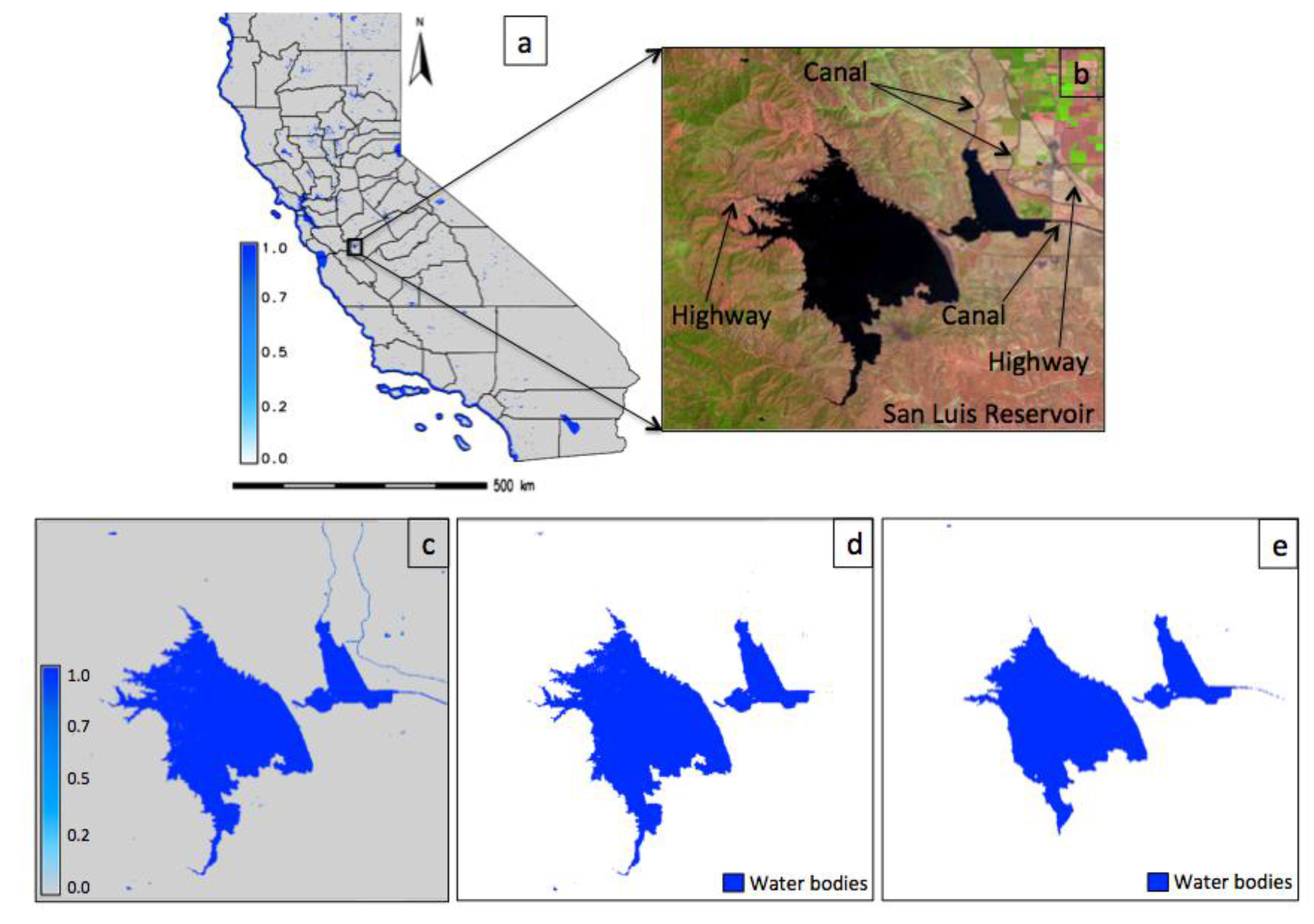
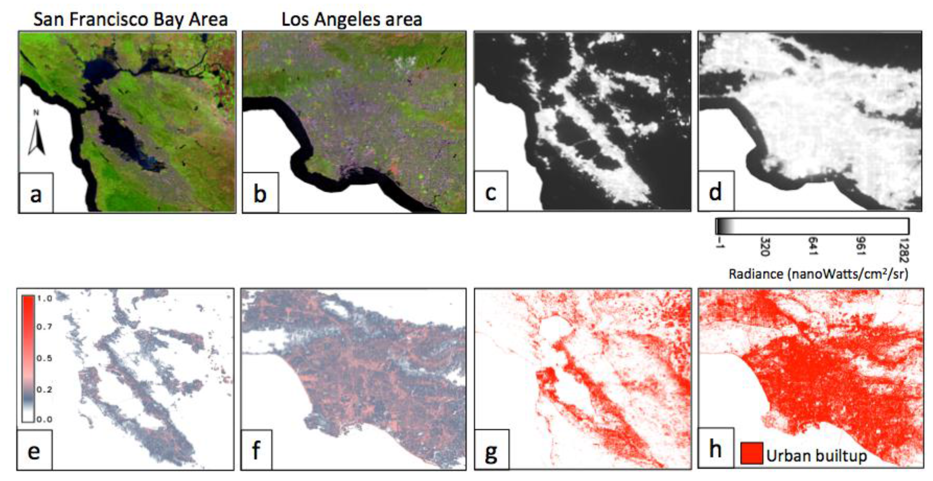
• Develop a method to utilize the abundance maps obtained from subpixel learning algorithms to retrieve fractional land cover (LC) classes representing forest, farmland (including agricultural and herbaceous lands), water, and urban areas.

We first present the qualitative and quantitative analysis of the subpixel learning algorithms to find out the best performing technique that renders fractional abundances of different classes with the highest accuracy through both computer-simulated and real-world data of an agricultural landscape and an urban scenario. These data were analyzed by deriving vegetation, substrate and dark objects (such as shadows and deep water) endmember fractions followed by comparison with the ground truth data for accuracy assessment using various measures. Subsequently, in the second part of this study, we show the scope of the best unmixing technique in an operational context to obtain global abundance maps from WELD (Web-Enabled Landsat Data) of the year 2011 using the global endmembers of substrate, vegetation and dark objects. The role of abundance maps in obtaining the fractional spatial extent of four LC classes such as forest, farmland, water bodies and urban areas is shown for the state of California, USA.

The paper is organized as follows: Section 2 briefly reviews the subpixel learning algorithms, Section 3 details the data and endmember generation, Section 4 discusses the LC classification methods and validation approaches, Section 5 presents the results and discussion, followed by concluding remarks in Section 6.

2. Review of Subpixel Learning Algorithms

The notion behind LMM is introduced below with a brief review of seven state-of-the-art subpixel learning algorithms. For each pixel, the observation vector y is related to endmember signature E by a linear model as

$$y=E\mathsf{\alpha }+\mathsf{\eta }$$

(1)

where, each pixel is a M-dimensional vector y whose components are the digital numbers corresponding to the M spectral bands. E = [e₁, …e_n-1, e_n, e_n+1 ..., e_N] is a M × N matrix, where N is the number of classes, {e_n} is a column vector representing the spectral signature of the nth target material and $\mathsf{\eta }$ accounts for the measurement noise. For a given pixel, the abundance of the nth target material present in the pixel is denoted by α_n, and these values are the components of the N-dimensional abundance vector $\mathsf{\alpha }$. We further assume that the components of the noise vector $\mathsf{\eta }$ are zero-mean random variables that are independent and identically distributed (i.i.d.). Therefore, the covariance matrix of the noise vector is σ²I, where σ² is the variance and I is M × M identity matrix.

2.1. Unconstrained Least Squares (UCLS)

The conventional approach to extract the abundance values is to minimize $\parallel y-E\mathsf{\alpha }\parallel$ as in (2):

$${\mathsf{\alpha }}_{\mathrm{UCLS}}={\left(E^{T}E\right)}^{-1}{E}^{T}y$$

(2)

which is termed a UCLS estimate of the abundance. UCLS with full additivity is a non-statistical, non-parametric algorithm that optimizes a squared-error criterion but does not enforce the non-negativity and unity conditions. Our previous study [31] compared the performance evaluation of UCLS, orthogonal subspace projection and singular value decomposition, which indicated similar unmixing results on different datasets. UCLS was faster in terms of execution time, therefore it is being considered here for comparison with constrained algorithms [32].

2.2. Fully Constrained Least Squares (FCLS)

To avoid deviation of the estimated abundance fractions, the ANC given in (3) and the ASC given in (4) are imposed on the model:

$${\mathsf{\alpha }}_n\ge 0 \forall n: 1\le n\le N$$

(3)

$${{\displaystyle \sum }}_{n=1}^N{\alpha }_n=1.$$

(4)

The ANC and ASC constrain the value of abundance in any given pixel between 0 and 1. When only ASC is imposed on the solution, the SCLS estimate of the abundance is

$${\mathsf{\alpha }}_{\mathrm{SCLS}}=E^T{E}^{-1}\left(E^{T}y-\frac{\mathsf{\lambda }}{2}1\right)$$

(5)

where

$$\mathsf{\lambda }=\frac{2\left(1^T{\left(E^{T}E\right)}^{-1}{E}^{T}y-1\right)}{1^T{\left(E^{T}E\right)}^{-1}1}.$$

(6)

The SCLS solution may have negative abundance values but they add to unity. FCLS [18,33] extends the NNLS (non-negative least squares) algorithm [34] to minimize $\parallel E\mathsf{\alpha }-y\parallel$ subject to $\mathsf{\alpha }\ge 0$ by including ASC in the signature matrix E by a new signature matrix (SME) defined by

$$SME=\left[\begin{array}{c}\mathsf{\theta }E\\ 1^T\end{array}\right]$$

(7)

with

$${\underset{\mathit{N}}{1=\left(\underbrace{\mathrm{11111..1}}\right)}}^T, \mathrm{and} s=\left[\begin{array}{c}\mathsf{\theta }y\\ 1\end{array}\right].$$

(8)

$\mathsf{\theta }$ in (7) and (8) regulates the ASC. Using these two equations, the FCLS algorithm is directly obtained from NNLS by replacing the signature matrix E with SME and pixel vector y with s. Further, the original NNLS algorithm was found to be computationally very slow in our experiments. Therefore, we modified the original FCLS by incorporating the faster NNLS proposed by [35].

2.3. Modified Fully Constrained Least Squares (MFCLS)

The ANC is a major difficulty in solving constrained linear unmixing problems as it forbids the use of Lagrange multiplier. Chang (2003) [18] proposed the replacement of ${\alpha }_n\ge 0\forall n:1\le n\le N$ with the absolute ASC (AASC), ${\displaystyle \sum }_{n=1}^N\left|{\alpha }_n\right|=1$. The AASC allows usage of Lagrange multiplier along with the exclusion of negative abundance values. This leads to an optimal constrained least squares solution satisfying both the ASC and AASC, which is called MFCLS and is expressed as

$$\underset{\alpha \in \Delta }{\min }\{(y-E\mathsf{\alpha }){\left(y-E\mathsf{\alpha }\right)}^T\}\mathrm{subject}\mathrm{to}\Delta =\{\alpha |{{\displaystyle \sum }}_{n=1}^N{\alpha }_n=1\mathrm{and}{{\displaystyle \sum }}_{n=1}^N\left|{\alpha }_n\right|=1\}$$

(9)

It turns out that the solution to (9) is

$${\widehat{\mathsf{\alpha }}}_{\mathrm{MFCLS}}={\widehat{\mathsf{\alpha }}}_{\mathrm{UCLS}}-{(E^{T}E)}^{-1}\left[{\mathsf{\lambda }}_{1}1+{\mathsf{\lambda }}_{2}sign\left(\alpha \right)\right]$$

(10)

where ${\widehat{\mathsf{\alpha }}}_{\mathrm{UCLS}}={(E^{T}E)}^{-1}{E}^{T}y$ as in (2). The ASC and AASC constraints are used to compute ${\mathsf{\lambda }}_1$ and ${\mathsf{\lambda }}_2$ by replacing $\alpha$ with ${\widehat{\alpha }}_{\mathrm{UCLS}}$ with the following constraints: ${{\displaystyle \sum }}_{n=1}^N{\alpha }_n=1^T\alpha =1,$ and ${{\displaystyle \sum }}_{n=1}^N\left|{\alpha }_n\right|=sign{\left(\alpha \right)}^T\alpha =1$, where $sign\left(\alpha \right)={\left({\omega }_1,{\omega }_2,\dots {\omega }_{n-1},{\omega }_n,{\omega }_{n+1}\dots {\omega }_N\right)}^T$ and

$${\omega }_n=\{\begin{array}{l}\frac{{\alpha }_n}{\left|{\alpha }_n\right|}; \mathrm{if} {\alpha }_n\ne 0\\ 0; \mathrm{if} {\alpha }_n=0\end{array}$$

(11)

MFCLS utilizes the SCLS solution and the algorithm terminates with all non-negative components.

2.4. Simplex Projection (SP)

SP finds the projection of a point onto a generic simplex and minimizes the least squares error while imposing the ANC and ASC. It reduces the computational complexity without any optimization, while recursively reducing the dimensionality of the problem to obtain a suitable abundance vector [2]. At each run, the algorithm identifies an endmember that has zero abundance and orthogonally projects on a hyperplane of a dimension less than the previous one. Considering P points $y_{\mathrm{p}}ϵ{ℝ}^{\mathrm{M}},\mathrm{p}=1,\dots ,\mathrm{P}$ with N endmembers {e₁, …e_n-1, e_n, e_n+1 , ... , e_N}, all points $y_{\mathrm{p}}$ are projected on to a simplex ${\mathrm{S}}_{\mathrm{I}}$ spanned by N in the set I = {e₁, …e_n-1, e_n, e_n+1 , ... , e_N} producing the projected points ${y^{\prime }}_{\mathrm{p}}$ and corresponding abundance vectors ${\widehat{\mathsf{\alpha }}}_{\mathrm{p}}=\left({\mathsf{\alpha }}_{\mathrm{p}1},\dots ,{\mathsf{\alpha }}_{\mathrm{pN}}\right)$. The projected points ${y^{\prime }}_{\mathrm{p}}$ are determined through ${y^{\prime }}_{\mathrm{p}}=E{\widehat{\mathsf{\alpha }}}_{\mathrm{p}}$ [36].

2.5. Sparse Unmixing via Variable Splitting and Augmented Lagrangian (SUnSAL)

Sparse regression [37] is related to both statistical and geometrical frameworks. The endmember search is conducted in a large library $E\in {ℝ}^{\mathrm{M}\mathrm{x}\mathrm{N}}$, where M < N and $\mathsf{\alpha }\in {ℝ}^N.$ Only a few of the signatures contained in E are involved in the mixed pixel spectrum, therefore $\mathsf{\alpha }$ contains many values of zero and is a sparse vector. The sparse regression problem is expressed as

$$\underset{\mathsf{\alpha }}{\min }{\parallel \mathsf{\alpha }\parallel }_0\mathrm{subject}\mathrm{to}\parallel y-E{\mathsf{\alpha }\parallel }_2\le \mathsf{\delta },\mathrm{subject}\mathrm{to}\mathit{\alpha }\ge 0,1^T\mathit{\alpha }=1$$

(12)

where ${\parallel \mathsf{\alpha }\parallel }_0$ denotes the number of nonzero components of $\mathsf{\alpha }$ and $\mathsf{\delta }\ge 0$ is the noise and modeling error tolerance. $\mathsf{\alpha }\ge 0\mathrm{and}$ $1^T\mathsf{\alpha }=1$ refers to the ANC and ASC, respectively. A set of sparsest signals belonging to the (N-1) probability simplex and satisfying error tolerance inequality defines the solution of (12). When the fractional abundances follow the ANC and ASC, the problem is referred to as constrained sparse regression given by (13) [38]:

$$\underset{\mathsf{\alpha }}{\min }\left(1/2\right)\parallel E\mathsf{\alpha }-{y\parallel }_2^2+\mathsf{\lambda }{\parallel \mathsf{\alpha }\parallel }_1\mathrm{subject}\mathrm{to}\mathit{\alpha }\ge 0,1^T\mathit{\alpha }=1$$

(13)

where ${\parallel \mathsf{\alpha }\parallel }_2$ and ${\parallel \mathsf{\alpha }\parallel }_1$ are the l₂ and l₁ norms and $\mathsf{\lambda }\ge 0$ is a weighing factor. SUnSAL is based on the alternating direction method of multipliers (ADMM) and is derived as a variable splitting procedure followed by the adoption of an augmented Lagrangian method [39].

2.6. SUnSAL and Total Variation (SUnSAL TV)

Sparse unmixing techniques do not deal with the neighboring pixels and tend to ignore the spatial context. SUnSAL TV takes into account spatial information (the relationship between each pixel vector and its neighbors) by means of the TV regularizer with an assumption that two neighboring pixels will very likely have similar fractional abundances for the same endmember [40]. The TV regularizer acts as a priori information and unmixing is achieved by a large non-smooth convex optimization problem.

2.7. Collaborative SUnSAL (CL SUnSAL)

Generally, the performance of sparse unmixing solution suffers from the limitation of a high degree of coherence between the signatures of the endmembers affecting the uniqueness of the solution. Collaborative sparse unmixing removes the above limitation where coherence has a weaker impact on unmixing since the pixels are constrained to share a small set of endmembers [10]. Here, the unmixing result is refined by solving a joint sparse regression problem in which the sparsity is simultaneously imposed on all the pixels [41]. Consider (1) while assuming P data points in matrix Y and $\mathsf{\eta }$ = [$\mathsf{\eta }$₁, …, $\mathsf{\eta }$_P] as the noise matrix. Assume ${\parallel \mathsf{\alpha }\parallel }_F\equiv \sqrt{\mathrm{trace}{\left\{\mathsf{\alpha }\mathsf{\alpha }\right\}}^T}$ is the Frobenius norm of $\mathsf{\alpha }$, and let $\mathsf{\lambda }>0$ be the regularization parameter, then the optimization problem is

$$\underset{\mathsf{\alpha }}{\min }\parallel E\mathsf{\alpha }-{Y\parallel }_F^2+\mathsf{\lambda }{{\displaystyle \sum }}_{k=1}^N{\parallel \alpha }^k\parallel {}_2\mathrm{subject}\mathrm{to}\mathsf{\alpha }\ge 0$$

(14)

where ${\mathsf{\alpha }}^k$ denotes the kth line of $\mathsf{\alpha }$. ${{\displaystyle \sum }}_{k=1}^N{\parallel \mathsf{\alpha }}^k{\parallel }_2$ is the l_2,1 mixed norm that supports a small number of nonzero lines and sparsity in $\mathsf{\alpha }$ among all the pixels, leading to the solution of (14) through the extended SUnSAL algorithm. CL SUnSAL solves the l₂ + l_2,1 optimization problem in addition to ANC. If ${\parallel \mathsf{\alpha }\parallel }_{2,1}={{\displaystyle \sum }}_{k=1}^N{\parallel \mathsf{\alpha }}^k{\parallel }_2$ denotes the l_2,1 norm, then (14) can be rewritten as

$$\underset{\mathsf{\alpha }}{\min }\parallel E\mathsf{\alpha }-{Y\parallel }_F^2+\mathsf{\lambda }{\parallel \mathsf{\alpha }\parallel }_{2,1}+{\iota }_{R+}\left(\mathsf{\alpha }\right)$$

(15)

where ${\iota }_{R+}\left(\mathsf{\alpha }\right)={{\displaystyle \sum }}_{i=1}^P{\iota }_{R+}\left({\mathsf{\alpha }}_i\right)$ is the indicator function. Equation (15) can be expressed in a constrained form and can be solved using the methods given in [42] to obtain the abundances. The abundance map allows a proportion of each pixel to be partitioned between classes. The value of abundance in any given pixel ranges from 0 to 1 (in an abundance map) with the number of abundance maps the same as the number of classes. The value 0 indicates absence of a particular class and 1 indicates the presence of only that class in a particular pixel. Intermediate values between 0 and 1 represent a proportion of that class.

3. Data

In this section, details about different experimental datasets, global Web-Enabled Landsat Data, and endmember generation are discussed.

3.1. Computer Simulated Data

One of the major problems in analyzing the quality of fractional estimation methods is that the exact ground truth information about the real abundances at subpixel level for all classes is difficult to obtain. Therefore, simulation of imagery is carried out as an intuitive way to perform evaluation of the techniques, for example, the simulated but realistic fully-calibrated citrus orchard virtual scene [43,44]. Since all the details of the simulated images are known, the algorithm’s performance can be examined in a controlled manner. For generating the synthetic multispectral data $y$ of six bands with different levels of noise $\mathsf{\eta }$, the linear mixture model $y=E\mathsf{\alpha } +\mathsf{\eta }$ was used with a simulated abundance map $\mathsf{\alpha }$. The noise was drawn from an uncorrelated normal distribution with zero mean and variance σ² (noise level). The endmembers E were taken from a set of global spectra of the three-endmember libraries [45]. At each pixel’s location in the simulated abundance map $\mathsf{\alpha }$, one specific endmember among the three was made dominant (abundance ≥ 0.77), and the remaining two abundance values were chosen at random such that all the values were positive and add to one. To have synthetic data closer to reality, the dominant endmembers had spatial correlation among the neighboring pixels for the same endmember except at region boundaries. In a separate set of experiments, σ² was increased in multiples of two (i.e., σ² was set to 2, 4, 8, …, 256) in order to analyze the performance of various learning algorithms on subpixel classification with variable noise.

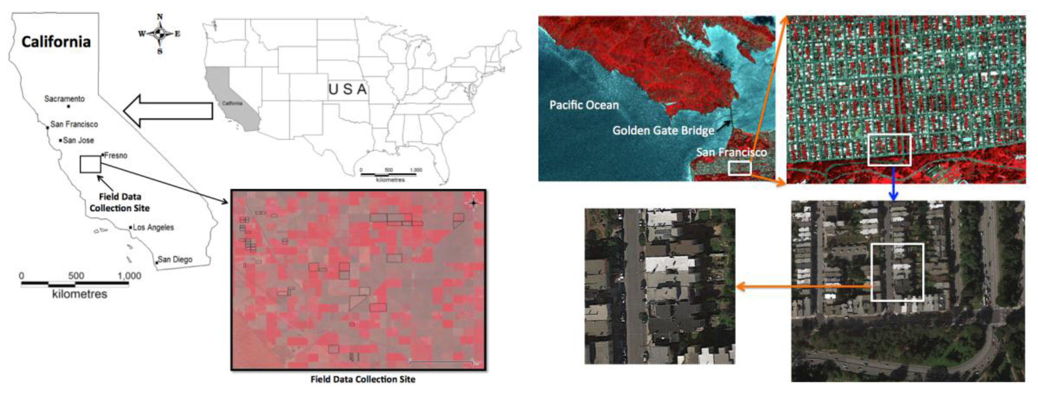
3.2. Landsat Data—An Agricultural Landscape and an Urban Scenario

A spectrally diverse collection of 11 time-series scenes of Level 1 (terrain-corrected), cloud-free Landsat-5 (obtained from the Web-Enabled Landsat Data (WELD) version 3.0 product) 16-bit data for Fresno, California, USA (WRS path 43, row 35) were used. These data were captured on 4 and 20 April, 22 May, 7 and 23 June, 9 and 25 July, 26 August, 11 and 27 September, and 13 October of the year 2008 and were calibrated to atmospheric reflectance [46]. The atmospheric reflectance was converted to surface reflectance by means of the 6S code implementation in LEDAPS (Landsat Ecosystem Disturbance Adaptive Processing System). For the ground truth data corresponding to the above scenes, a coincidental set of ground canopy covers were collected for a number of surveyed fields that were located within an area of about 25 × 35 km² southwest of the city of Fresno (Figure 1). A total of 74 polygons of fractional vegetation cover were generated from digital photographs taken with a multispectral camera mounted on a frame at nadir view pointed 2.3 m above the ground. These photographs were acquired at the commercial agricultural fields of the San Joaquin Valley (in central California) on the 11 dates mentioned above, except for one date when the Landsat acquisition preceded the ground observation by one day. For each date, 2–4 evenly spaced pictures were taken for an area of 100 × 100 m² with center location marked by GPS [47]. These fractional measurements belonged to a diverse set of seasonal and perennial crops in various developmental stages, from emergence to full canopy, that represented an agricultural environment in the real-world scenario.

A second set consisting of a pair of coincident clear sky Landsat TM-5 data and WV-2 data (World View-2 of 2 m spatial resolution) for an area of San Francisco, California, USA were used to assess the algorithms. San Francisco was chosen for the test site because of its urbanized landscape, with a mix of building architectures, vegetation and substrate. WV-2 data were acquired a few minutes after the Landsat-5 TM data acquisition on 1 May 2010 for an area near the Golden Gate Bridge, San Francisco (Figure 1). The spectral range of the first four bands of Landsat data correspond to the WV-2 bands 2, 3, 5 and 7, so they have similar spectral response functions. WV-2 data were converted to top of atmosphere reflectance values. The Landsat unmixed images were compared to the corresponding WV-2 fraction images for accuracy assessment.

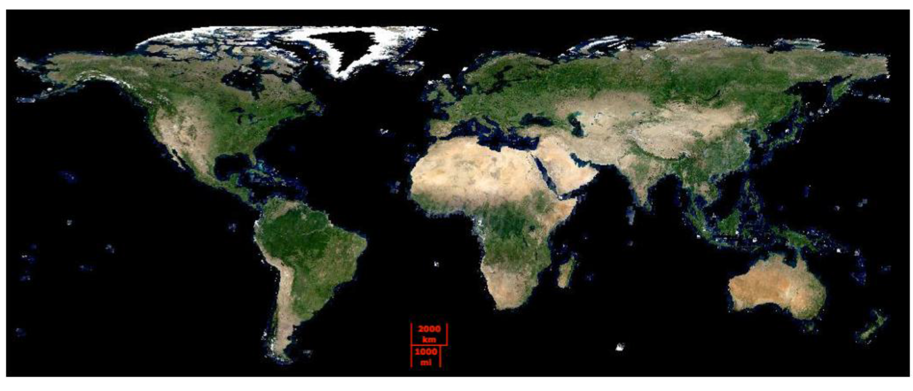
3.3. Global Web-Enabled Landsat Data (WELD)

The NASA-funded WELD, through the Making Earth System Data Records for Use in Research Environments (MEaSUREs) project, has been systematically generating 30 m monthly and annual global composite products from Landsat 7 ETM+ and Landsat 5 TM data for all non-Antarctic land surface mosaics [48]. The entire globe is covered with around 8000 scenes/month and the version 3.0 global WELD (shown in Figure 2) are available in public domain for a three year period from 2008 to 2011 (~0.3 million scenes), spectrally calibrated and converted to surface reflectance and brightness temperature.

3.4. Endmember Generation

Global mixing spaces using a spectrally diverse LC and a diversity of biomes with 100 Landsat ETM+ subscenes were used to define a standardized set of spectral endmembers of substrate (“S”—endmember 1), vegetation (“V”—endmember 2), and dark objects (“D”—endmember 3) that spans all terrestrial biomes determined by mean annual temperature and precipitation in proportion to land area [49]. The geographical locations of the 100 Landsat scenes showing spectral diversity resulting from LC variety across biomes was established in an earlier study [50]. The subscenes included within-scene spectral variability, LC transition and global land area distribution. With a linear stretch of 2% applied to the bands within a subscene, substrate, vegetation and water were apparent as brown, green and black color, respectively. The substrate includes urban structures, soils, sediments, rocks, and non-photosynthetic vegetation. Vegetation refers to green photosynthetic plants, and dark objects encompasses absorptive substrate materials, clear water, deep shadows, etc. The S-V-D endmember coefficients with dates and locations for each subscene are available in [45] and a plot of the endmembers is provided in [50]. The estimates obtained from the global endmembers have been compared to the fractional vegetation cover derived vicariously by linearly unmixing near-coincidental WV-2 acquisitions over a set of diverse coastal environments, using both global endmembers and image-specific endmembers to unmix the WV-2 images. The strong 1:1 linear correlation between the fractions obtained from the two types of image indicate that the mixture model fractions scale linearly from 2 m to 30 m over a wide range of terrains. When endmembers are derived from a large-enough sample of radiometric responses to encompass the Landsat spectral mixing space, they can be used to build a standardized spectral mixture model for global mapping applications.

4. Classification Methods and Validation Approaches

In this section, classification methods, validation datasets and validation approaches, along with the algorithm’s parameter settings and computational requirements are discussed.

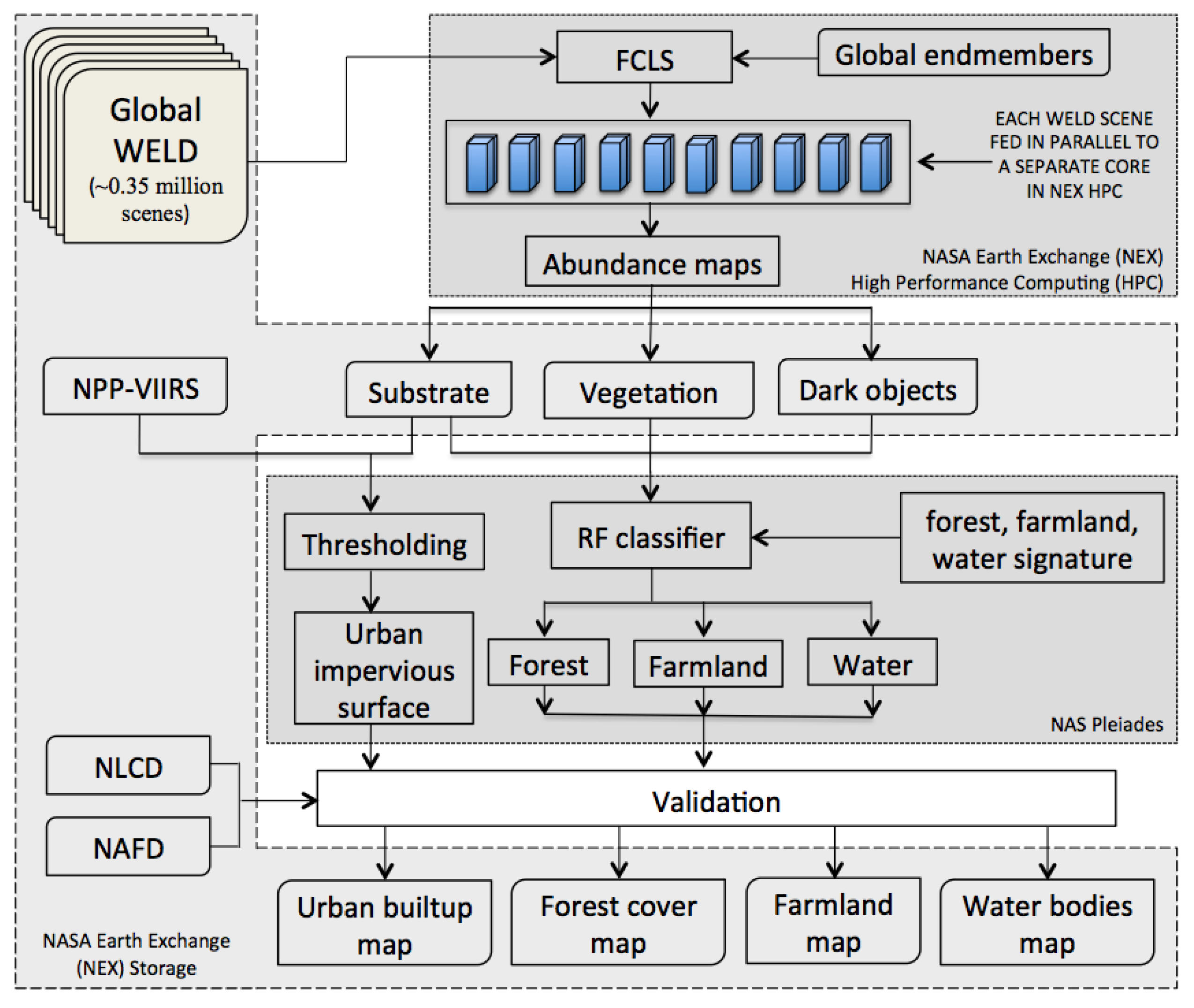
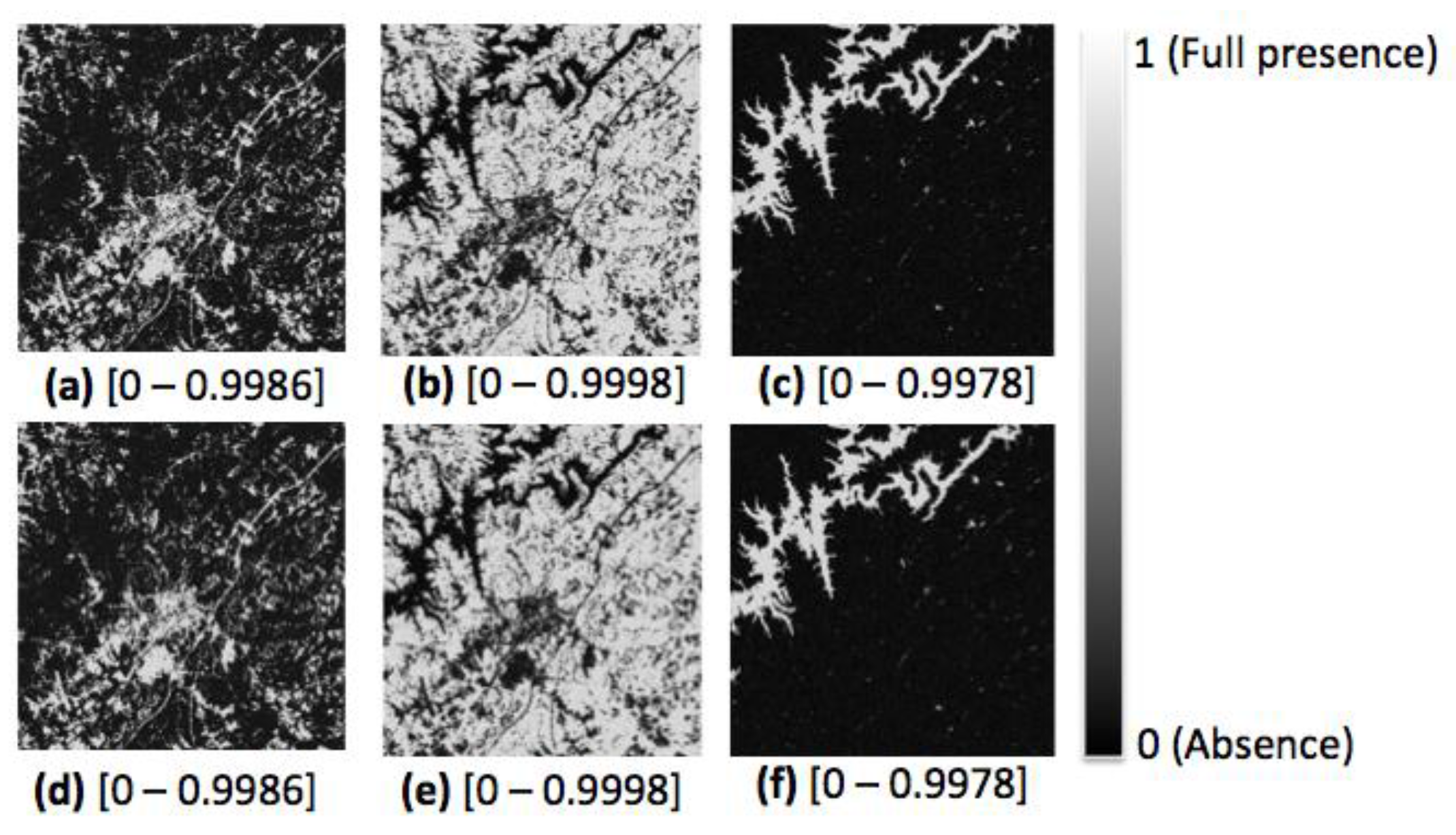
4.1. Land Cover Classification from Abundance Maps

Subsequent levels of classification can be carried from the S-V-D abundance maps to obtain fractional maps of forest, farmland/grassland, water bodies and urban areas, etc. for numerous other applications. In the S-V-D abundance maps, dense forest pixels occur on and near the binary mixing trend between vegetation and dark (i.e. shadow) endmembers. The vegetation endmembers generally correspond to illuminated foliage. The higher the fraction of vegetation endmember, the less canopy shadow and illuminated substrate contribute to the pixel’s reflectance. Herbaceous vegetation (grass) typically has less canopy shadow than closed canopy forest, so they occur closer to vegetation endmember (higher vegetation fractions). A continuum may exist between dense forest and herbaceous vegetation using a trade-off between vegetation and shadow fractions. Dense forest can be distinguished from farmland/grassland by assigning a threshold to both the vegetation and dark endmember fractions. Additionally, NDVI (Normalized Difference Vegetation Index) values can also be used as a supplement layer for discriminating dense forest by applying a suitable threshold. Sampled forest patches for training data revealed that vegetation abundance >0.2, dark objects abundance >0.6 and NDVI >0.7 represented forest areas.

In this work, the above approach is tested for the state of California in the United States for which training, test and relevant ancillary data were available. For classification of the three LC classes, 200,000 pixels belonging to homogeneous dense forest, homogeneous herbaceous vegetation/grassland, and water bodies (clear water, turbid water and green water caused by eutrophication) were selected as training samples using a stratified random sampling on the basis of administrative boundaries. The forest and grassland pixels were also confirmed by following the method in Huang et al., (2008) [51] and by visual interpretation of the high-resolution Google Earth^TM images. A supervised classification was performed on S-V-D abundances using the random forest (RF) classifier [52] into dense forest, farmland and water bodies. Figure 3 shows the flowchart of the overall methodology. The same set of training polygons were also used to generate training samples to classify the original WELD data (bands 1‒5 and 7) to obtain per-pixel classified maps in order to assess the advantages of fractional maps over per-pixel classification. Here, the number of trees was set to 250, the node size was set to five and the maximum number of terminal nodes was set to 500. When further parameter variations did not increase the accuracy, the final values of the parameters were obtained empirically depending on the minimum execution time and memory requirements.

For the classification of built and constructed impervious surfaces (such as buildings, driveways, sidewalks, roads, parking lots and other man-made surfaces), the common sources of error include underestimation in areas with extensive tree cover and overestimation in areas with extensive bare ground. In this regard, Defense Meteorological Satellite Program Operational Line Scanner (DMSP OLS) nighttime light data and the Visible Infrared Imaging Radiometer Suite (VIIRS) day–night band (DNB) carried by the Suomi National Polar-Orbiting Partnership (NPP) satellite are very useful in monitoring and analyzing human activities and natural phenomena. DMSP OLS and NPP-VIIRS pixels in the nighttime light images aid in classifying urban built-up areas since they capture illuminated surfaces than the surrounding dark areas at night [53].

Pixels with radiance values equal to or larger than a threshold that produces minimum difference between image-derived value and reference data are considered part of an urban built-up area [54]. In this study, the NPP-VIIRS data at a resolution of 15 arcsec grids obtained from the NOAA (National Oceanic and Atmospheric Administration) National Geophysical Data Center were resampled to 30 m. A threshold of the minimum value radiance was used to segment the images into urban and non-urban areas for different cities. The absolute difference between the extracted area and the reference data was recorded and the process was repeated by varying the threshold to reach the maximum pixel value of the image. The threshold value that produced minimum difference was selected for urban built-up area extraction. For each city, FCC (false color composite) of urban areas was also adopted to analyze the spatial coherence of the extracted results.

4.2. Validation Methods

For the computer-simulated data, the estimated class abundance maps were first compared with the simulated true abundance maps using visual checks. Performance discriminators such as range of fractional estimates (minimum and maximum abundance values), correlation coefficient (r), RMSE (root mean square error), signal-to-reconstruction error (SRE), probability of success ($p_s)$, and bivariate distribution function (BDF) were used for validation. A smaller RMSE indicates a better unmixing result i.e., higher accuracy. SRE and $p_s$ were computed for each algorithm for various noise levels [37]. The quality of the reconstruction of a spectral mixture is measured using $\mathrm{SRE}\equiv E{[\parallel \alpha \parallel ]}_2^2/E[\parallel \alpha -{\widehat{\alpha }\parallel }_2^2]$ in decibels, where $\mathrm{SRE}\left(\mathrm{dB}\right)\equiv 10{\log }_{10}\left(\mathrm{SRE}\right)$. It gives information by relating the power of the error to the power of the signal. It is to be noted that the higher the SRE(dB), the better the unmixing performance.$p_s\equiv P\left(\frac{\parallel \widehat{\alpha }-{\alpha \parallel }^2}{{\parallel \alpha \parallel }^2}\le \mathrm{threshold}\right)$, where $p_s$ is an estimate of the probability that the relative error power is smaller than a certain threshold and is also commonly used in the sparse regression community. It indicates the stability of the estimation, which is a complimentary measure to SRE (that is an average). BDF is used to visualize the accuracy of prediction by mixture models. Points along a 1:1 line on the BDF graph indicate predictions that match completely with the real abundances. Additionally, for each of the 74 surveyed field locations in the 11 Landsat scenes of the agricultural landscape, mean absolute error (MAE) was computed for all the subpixel learning algorithms.

Comprehensive validation of the entire fractional LC maps of the forest, farmland, water and urban areas was found to be extremely challenging as there are still limited datasets that can be used as a reference. Therefore, we focused on the National Land Cover Database 2011 (NLCD 2011) [55], NLCD 2011 percent tree canopy cover, NLCD 2011 percent developed imperviousness [56], North American Forest Dynamics (NAFD) 2010 product [56,57,58], and Google Earth^TM imagery for both qualitative and quantitative methods. Qualitative validation included comprehensive visual assessment with local reference of high spatial resolution Google Earth^TM imagery, whereas quantitative methods included a design-based accuracy assessment with NLCD 2011 products. For the quantitative assessment, the validation points were stratified into four groups based on NLCD 2011 LC classes: (1) Forest (NLCD classes: deciduous forest, evergreen forest, mixed forest, and woody wetland); (2) Agriculture/farmland (NLCD classes: grassland/herbaceous, pasture/hay, and cultivated crops); (3) Water (NLCD class: open water); and urban (NLCD classes: developed, open space, low intensity, medium intensity, and high intensity). Additionally, a separate per-pixel classified map from WELD was used for comparison with the fractional class maps. A total of 200,000 sampling pixels were chosen at random from 1000 validation sites for each LC type. Pixels with more than 50% presence of any class in the fractional maps were discretized to the respective class, although this threshold can be reduced if a smaller fraction of LC class is to be accounted. For urban areas, pixels with more than 30% fractions were considered to be urbanized, since urban areas have a mix of houses, parking spaces, walkways, lawns and roads. The per class producer’s accuracy (PA), user’s accuracy (UA), overall accuracy (OA), and kappa coefficient were calculated by comparing fractional maps with NLCD 2011 LC map and averaged over 10 iterations.

4.3. Parameter Settings and Computational Requirements

All the above subpixel learning algorithms (discussed in Section 2) were implemented in MATLAB^®. In FCLS, the tolerance was set to $1\times {10}^{-5}$ (the algorithms will converge at this value without entering an infinite loop) and the value of $\mathsf{\lambda }$ (weightage for the sum to one constraint) was set to 20, which was determined empirically. The tolerance in MFCLS was set to $1\times {10}^{-7}$. The parameter $\mathsf{\lambda }$ in SUnSAL was set to ${10}^{-5}$, $\mathsf{\delta }={10}^{-4}$; $\mathsf{\lambda }$ in SUnSAL TV was set to $5\times {10}^{-4}$ and ${\mathsf{\lambda }}_{\mathrm{TV}}$ in SUnSAL TV was set to $5\times {10}^{-3}$ for computer-simulated data and ${10}^{-3}$ for the Landsat data. $\mathsf{\lambda }$ in CL SUnSAL was set to ${10}^{-2}$ for both without and with the ASC and ANC activated. Here, the optimal parameter values were obtained after several experiments with various values of $\mathsf{\lambda }$ and ${\mathsf{\lambda }}_{\mathrm{TV}}$ (see Tables IV–V in [37]; Tables I–II in [10,40]) and were finalized based on the higher SRE. It was observed that our observations of the best parameter values coincided with the values in [37,39]. The maximum number of iterations was set to 100 and all other parameters were set to default. UCLS and SPU do not require any parameter settings.

In order to provide an open source solution and attain high execution speed for the global WELD classification, FCLS MATLAB^® implementation was converted to C++ syntax along with other open source packages such as OpenCV (Open Source Computer Vision) package, boost C++ libraries, gdal, and GRASS (Geographic Resources Analysis Support System) GIS on the NASA Earth Exchange (NEX) platform. The NEX framework combines state-of-the-art supercomputing (Pleiades supercomputer), Earth system modeling, remote sensing (RS) data from NASA and other agencies, workflow provenance, and a scientific social networking platform to deliver a complete end-to-end work environment. Since NEX is built upon the terrestrial observation and prediction system (TOPS) [59], a data assimilation and modeling framework developed at the NASA Ames Research Center, it provides software libraries and tools required by NEX to automate the processing of satellite and climate data, and manages workflows for data analysis and modeling studies. Each node in the Pleiades Harpertown compute cluster have CPUs consisting of 8 GB of memory and eight cores with 3-GHz processors per node. The deployment of the algorithm was done through the QSub routine and the message passing interface. Each WELD tile was fed to a separate core in parallel in the NEX high performance computing platform.

5. Experimental Results and Discussion

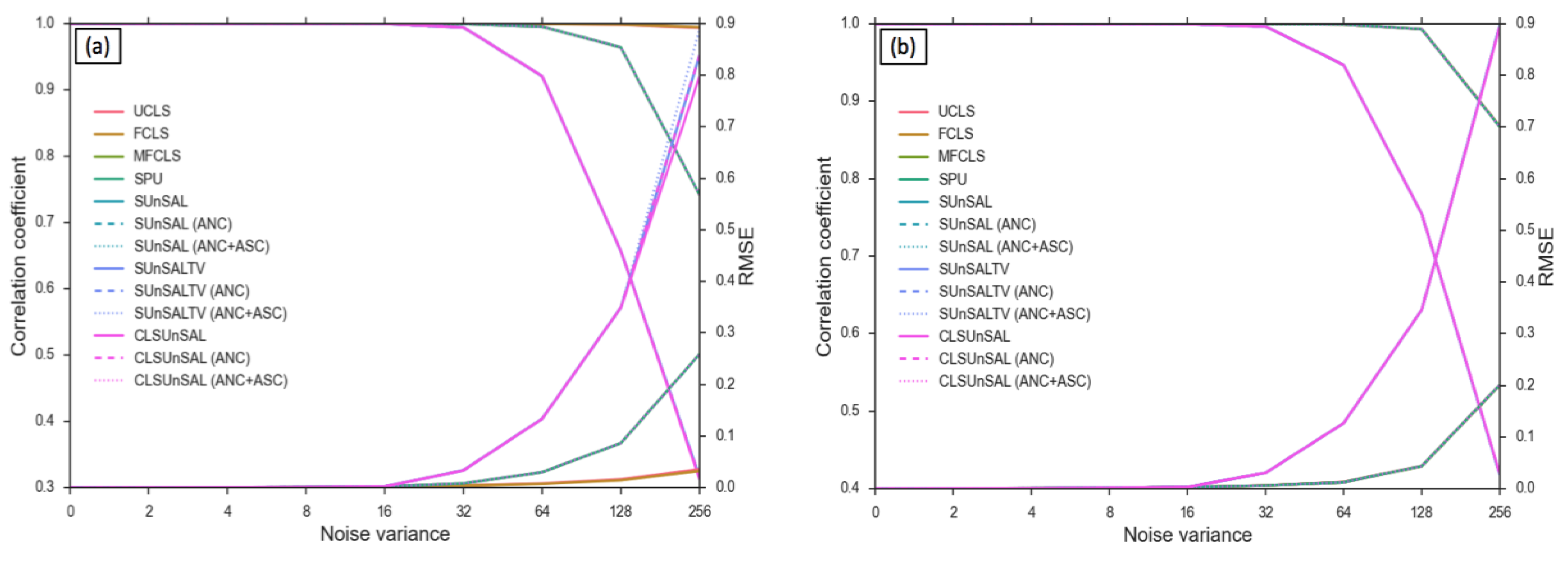
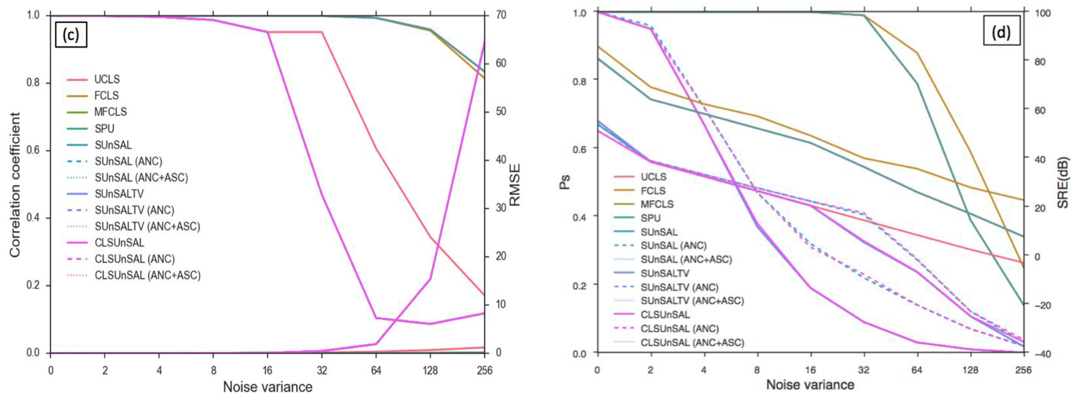
5.1. Computer Simulations

Figure 4a–c shows noise-free synthetic abundance maps for endmember 1, 2 and 3 and Figure 4d–f shows estimated abundance maps obtained for each signature class from FCLS, with the range of abundance fraction values underneath each panel. Note that the range of abundance values obtained from FCLS is exactly the same as in the synthetic abundance maps indicating that FCLS has been able to accurately perform subpixel classification. Results from the other algorithms are not presented due to space considerations. Visual examination of the abundance maps obtained from the seven algorithms revealed that they were similar in terms of the relative fractions and from the detection point of view.

Figure 5a–c shows r (statistically significant at 0.99 confidence level, p-value < 2.2 × 10⁻¹⁶) and RMSE between real abundance and estimated abundance obtained from the seven algorithms for all the three endmembers corresponding to different levels of noise. For SUnSAL, SUnSAL TV and CL SUnSAL algorithms, three different cases—without any constraints, with ANC, and with both ANC and ASC imposed on the optimal solution were evaluated. For the noise-free data, most of the models had high r (close to 1) and low RMSE. All the models were robust until noise variance 32, beyond which r gradually decreased and reached a minimum of 0.12, producing higher RMSE following a hyperbolic curve. FCLS was robust until noise variance 128 for all the three endmembers and it showed highest r for endmember one at noise variance 256. For endmembers two and three, FCLS, MFCLS, SPU, SUnSAL (ANC + ASC) and CL SUnSAL (ANC + ASC) produced the highest r with lower RMSE. Figure 5d shows the plot of $p_{\mathrm{s}}$ and SRE(dB) against various noise levels. Abundance values obtained from the unmixing algorithms were accepted when $\parallel \widehat{\alpha }-{\alpha \parallel }^2/{\parallel \alpha \parallel }^2\le$ threshold, where threshold (0.0005) is the 99th percentile of $\parallel \widehat{\alpha }-{\alpha \parallel }^2/{\parallel \alpha \parallel }^2$ of FCLS abundance at noise variance 32, where most of the methods rendered good performance. Figure 5d reveals that until noise variance 32, FCLS, MFCLS, SPU, fully-constrained SUnSAL and CL SUnSAL had $p_s$ close to 1, beyond which they decreased gradually. FCLS was robust even at noise variance 128 with $p_s$ = 0.6. With respect to SRE(dB), FCLS was better among all the algorithms at different noise levels. On the other hand, UCLS, SUnSAL (no constraints), CL SUnSAL (no constraints), along with SUnSAL TV (without and with constraints) had poor performance with low r, high RMSE, low $p_s$ and SRE. The plot of the execution time taken by each of the algorithms for unmixing computer-simulated data for different levels of noise on a 2.53 GHz Intel Core i5 processor with 8 GB RAM revealed that UCLS, FCLS, MFCLS, SPU and SUnSAL took much less execution time (<3 s), whereas SUnSAL TV and CL SUnSAL took higher execution time (15 s and 7 s respectively). The points on the BDF plots (not shown here) fell almost in a 1:1 line for all the three endmembers. As the noise variance increased, the estimated abundance deviated from the real abundance values.

Considering the various measures of performance discriminators and execution time in the above analysis, it was found that overall, FCLS outperformed, followed by MFCLS, SPU and SUnSAL with marginally lower accuracies. Even though SUnSAL TV introduces regularization to enforce continuity of abundances among neighboring pixels, it performed the worst of all, with poor accuracy measures and higher execution times. In the next section, the implementation of the algorithms on real-world data for different landscapes are discussed.

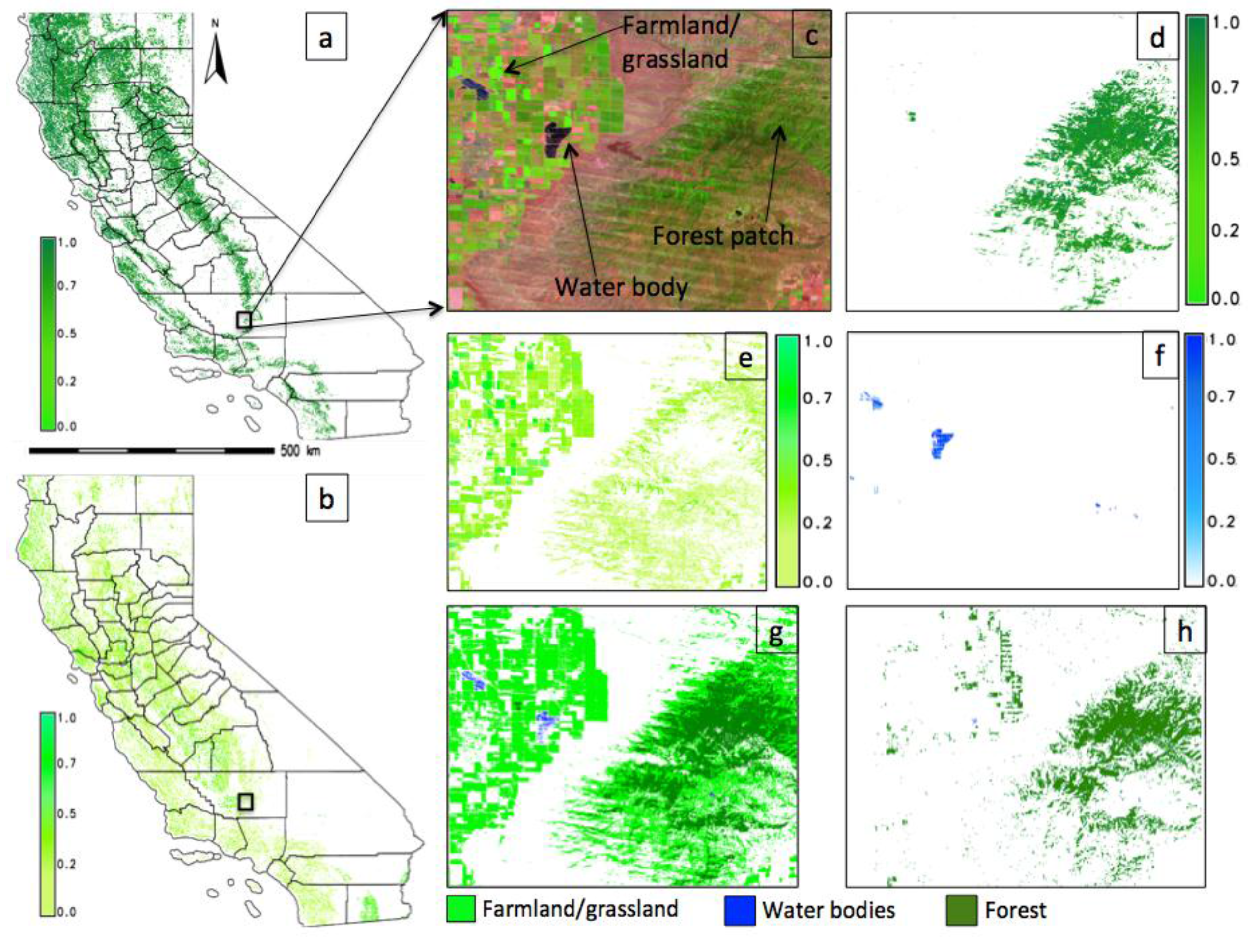
5.2. Landsat Data—An Agritultural Landscape

Each of the 11 Landsat scenes was unmixed with S-V-D endmembers using different models to obtain the abundance estimates. For each scene, the vegetation abundances were compared with ground-based measurements. FCLS produced the least MAE of 0.03 and highest r of 0.99. All other methods except fully-constrained SUnSAL TV produced a lower MAE of 0.08 and r of 0.98. SUnSAL TV (ANC+ASC) rendered high MAE (0.3) and low r (0.21). FCLS was slightly better when compared to the other methods. On an average, FCLS took the minimum execution time (20 min) to process each Landsat scene (7321 rows × 8367 columns). SUnSAL and CL SUnSAL rendered good classification accuracies with high execution time (7200 s (2 h)/scene). Although time exhaustive (the algorithm took 118,800 s (33 h)/scene), SUnSAL TV did not produce satisfactory results.

5.3. Landsat Data—An Urban Scenario

Unmixed Landsat and WV-2 data of San Francisco with the S-V-D endmembers were compared for accuracy where each 2 m WV-2 pixel is less than 0.5% of the area within the 30 m full-width, half-maximum of the Landsat point spread function. The WV-2 fractions were convolved with a Gaussian low pass filter with the point spread function of the Landsat sensor and resampled to 30 m. Coordinate comparison of the WV-2 and Landsat datasets at many random pixels did not reveal any systematic image registration error. Validation revealed that the unconstrained and partially constrained algorithms viz. UCLS, SUnSAL, SUnSAL TV and CL SUnSAL for the S, V and D classes produced MAE of 0.11, 0.07 and 1.99, respectively, and r of 0.86, 0.88 and −0.03, respectively. FCLS for S, V and D classes showed MAE of 0.03, 0.02 and 0.02, respectively, and r of 0.94, 0.97 and 0.97, respectively, producing the best classification results with the smallest execution time (19 min) to process each Landsat scene (7151 rows × 8241 columns). The SUnSAL family of algorithms was the most time-exhaustive (SUnSAL and CL SUnSAL took 7200 s (2 h)/scene), while fully-constrained SUnSAL TV (for which the execution time was 118,800 s (33 h)/scene) did not produce reasonable results.

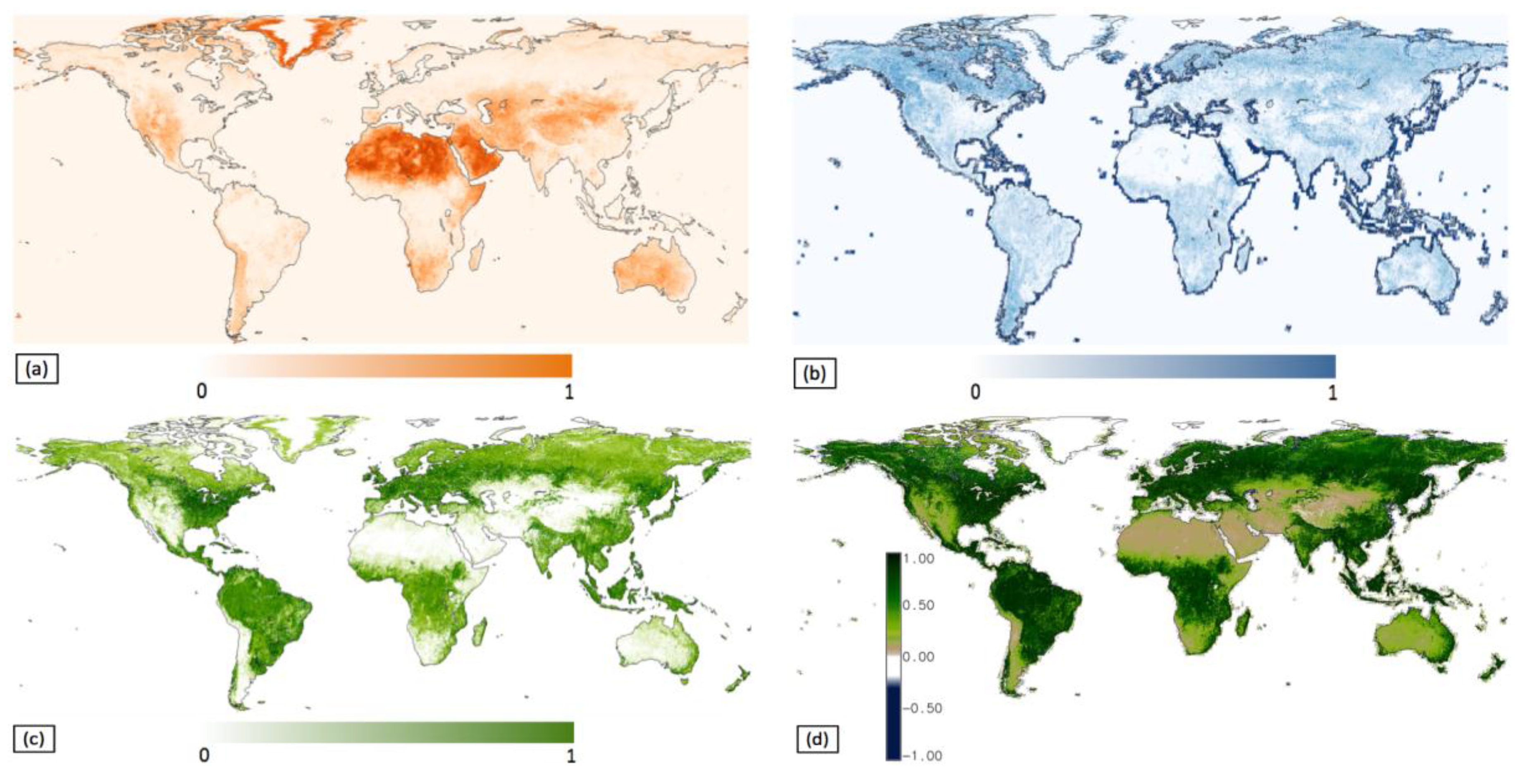
5.4. Global WELD Subpixel Classification

Figure 6 is a mosaic of 8003 scenes showing the global (a) substrate, (b) dark objects, (c) vegetation abundance map and (d) NDVI generated from 2011 annual WELD. Each WELD scene is composed of 5295 rows and 5295 columns, therefore, a single snapshot of global data consists of 224.3 billion pixels with six spectral dimensions, processed in 29 min utilizing 200 cores.

Note the correspondence between the vegetation abundance and NDVI, which clearly indicates that the vegetation endmember was able to extract the vegetation component from the mixed pixels when investigated visually and spatially. To our best knowledge, this is the first attempt to produce time series global abundance maps at the native 30 m spatial resolution. With the extended WELD project, monthly and annual global products for six three-year periods spaced every five years (1985, 1990, 1995, 2000, 2005 and 2010) are planned in reverse chronological order (i.e., 2010, ..., 1985).

5.5. Subpixel Land Cover Classification

An elementary implementation of our framework produced reasonable results. Figure 7a,b shows the fractional forest cover and farmland/grassland maps of California. Figure 7c shows FCC (bands 3‒5) for a small region from south-central California where dense forest pixels are highlighted in dark green, farmland as light green and water bodies in black. Figure 7d–f are the fractional LC maps of the three classes, Figure 7g is the classified output from RF classifier and Figure 7h is the forest cover map from NAFD. By comparing Figure 7d,g,h through visual inspection, it is clear that although RF seems to correctly classify the pixels, it has overestimated the classes because of per-pixel classification, while the NAFD product has overestimated forest areas over farmland. Figure 8a shows the spatial distribution of fractional water bodies and Figure 8b is a FCC of the San Luis Reservoir, with canals and highways along the water body. Figure 8c is the fractional water map, Figure 8d shows the classified map from RF and Figure 8e is the water body as depicted in the NAFD map. Linear canals have also been detected along with the reservoir in the unmixing based classification, unlike the output from the RF and NAFD product.

Figure 9a,b shows the RGB composites (bands 3‒5) for the San Francisco (SF) Bay Area, popularly known as Silicon Valley, and the Los Angeles (LA) area, Figure 9c,d is corresponding NPP-VIIRS nighttime data, Figure 9e,f is the fractional urban built-up areas obtained using the combination of substrate and nighttime light data, and Figure 9g,h shows the corresponding built-up area obtained from the classification of original WELD bands using RF.

It is clear that RF has overestimated the urban built-up areas since it also classifies open areas as urban within and outside the urban extent, causing high commission errors. If large open areas are separated from the urban areas during classification, it will decrease the total urban extent, especially when a definite urban boundary is not defined, as in the case of the SF Bay Area.

The minimum fractional forest cover estimated was 0.0016 ha (16 m²) and the total fractional area of forest cover was found to be 8,324,716 ha (19.7%). RF produced 8,978,601 ha (21.18%), NAFD showed 11,672,365 ha (27.53%), the NLCD 2011 LC map indicated 9,550,523 ha (22.54%) and the NLCD forest canopy percent indicated 7,456,588 ha (17.56%). For the farmland/grassland fraction map, the minimum fractional cover was 0.002 ha (20 m²) and the total fractional area was found to be 2,439,087 ha (5.8%), RF had 2,937,550 ha (6.9%), and NLCD showed 3,337,367 ha (7.8%). For farmland, the reason for the difference among NLCD, unmixing and RF could be the seasonal growth cycles in croplands. NLCD considers these classes as cultivated crops, which appear similar to farmland/herbaceous vegetation. The minimum fraction of water detected was 0.0036 ha (36 m²), which may correspond to small pools in residential areas. Unmixing-based classification estimated 1,888,727 ha (4.46%), RF yielded 1,948,956 ha (4.60%), NAFD indicated 1,769,822 ha (4.17%), and the NLCD 2011 LC map had 1,938,462 ha (4.57%) as the water spread area. NAFD underestimated water bodies, as also seen in Figure 8e, while RF and NLCD had closer values.

For the SF Bay Area, unmixing-based classification using VIIRS data showed 139,152 ha as urban areas (most of the pixels have impervious surface fractions between 15 and 55%), RF gave a much higher estimate of 235,471 ha, NLCD indicated 231,179 ha, and the NLCD percent developed imperviousness layer had 141,522.73 ha (most of the pixels have impervious surface fractions between 40 and 70%). One reason for the difference in the range of impervious surfaces between unmixing and NLCD impervious product could be the underlying methods: FCLS (used in unmixing) versus regression tree (used in NLCD). Also, FCLS imposes a sum-to-one constraint on the endmembers, whereas NLCD method does not. For the urban impervious surface in the LA area, unmixing-based classification yielded 189,179 ha, RF gave 315,496 ha, NLCD LC map resulted in 313,622 ha and the NLCD percent developed impervious layer indicated 191,134 ha. It can be seen that the unmixing and NLCD impervious percent values were very close. However, hard classification almost always overestimated the LC area compared to the fractional maps. These results also show that unmixing provides a physical basis to quantify the spectral characteristics of LC and distinguish spectrally heterogeneous areas from more spectrally homogeneous LC. One benefit of defining urban extent on the basis of spectral heterogeneity is the ability to generate a range of verifiable extent estimates that encompass a range of different definitions of urban areas, given that a unique spectral signature for urban LC is difficult to obtain. The above approach attempts to eliminate ambiguity resulting from varying administrative and political definitions of urban areas, as in many cases the exact definition of urban/non-urban remains ambiguous. As such, whether a park near the Golden Gate Bridge in San Francisco is urban or non-urban remains a question. It is to be noted that the park was classified as non-built-up in the original WELD data using RF. Beyond this, the lights in the park also contribute to the light emissions of the city.

Validation—For each of the 1000 validation sites as shown in Figure 10, (each point represents ~10 validation sites) reference datasets were derived for each LC type to create a confusion matrix. The results are tabulated in

Table 1. Confusion matrix.

	Forest	Farmland	Water	Urban (SF)	Urban (LA)	Overall
Total samples	200,000	200,000	200,000	100,000	100,000	800,000
Class samples	100,000	100,000	100,000	50,000	50,000	400,000
Non-class samples	100,000	100,000	100,000	50,000	50,000	400,000
Unmixing TPR *	93.87	90.29	92.65	89.81	90.83	91.49
Unmixing FPR *	3.46	4.12	0.5	4.99	8.17	4.25
RF TPR *	88.86	85.19	88.27	83.33	79.91	85.11
RF FPR *	5.12	8.21	2.17	12.71	15.13	8.67

* TPR—True positive rate, FPR—False positive rate, RF—Random Forest.

, which indicates that unmixing-based classification produced a higher overall TPR (true positive rate) of 91%, which is more than the per-pixel classification using RF (85%).

Table 2. Classification accuracy assessment.

	RF		Unmixing Based Classification
Class	PA **	UA **	PA **		UA **
Forest	87.97	88.69	91.17	$\uparrow$	95.29	$\uparrow$
Farmland	85.11	86.75	94.87	$\uparrow$	85.63	$\downarrow$
Water	89.87	87.43	89.65	$\downarrow$	95.12	$\uparrow$
Urban (SF)	84.24	83.19	85.33	$\uparrow$	94.31	$\uparrow$
Urban (LA)	76.52	83.39	88.67	$\uparrow$	92.96	$\uparrow$
Average	84.74	85.89	89.94	$\uparrow$	92.66	$\uparrow$
OA **	85.31		91.30
kappa	0.83		0.89

** PA—Producer’s accuracy, UA—User’s accuracy, OA—Overall accuracy.

indicates PA and UA. The OA and kappa for unmixing-based classification (91.30% and 0.89) was higher than the RF classifier (85.31% and 0.83%). While the RF class areas are close to NLCD maps, it has wrongly classified many pixels belonging to barren/open land as built-up. Few water pixels were wrongly classified using unmixing-based classification, therefore, the PA decreased marginally. This is because some confusion between water and shadow might appear since both classes have pixels which are very dark in all the spectral channels. However, given the same geo-coordinates of training pixels for classification, the UA increased from 87.43 to 95%. The PA increased for forest (3.2%), farmland (9.76%), urban built-up (SF) (1.09%), urban built-up (LA) (12.15%), and the UA increased for forest (6.6%), water bodies (7.7%), urban built-up (SF) (11%), urban built-up (LA) (9.6%) in the unmixing based classification output. On the other hand, the UA decreased (∼1%) for farmland.

Unmixing was intended to improve classification accuracies by correctly classifying pixels, which were likely to be misclassified by RF classifier. Therefore, a cross-comparison of the two classified images located the pixels that were assigned different class labels at the same location. These wrongly classified pixels when validated revealed a 6% (29,830,877 pixels) improvement in unmixing-based classification. Had the WELD data been classified using a hard classification technique such as RF, the errors would accumulate for all the pixels.

Pixel to pixel correlation between the unmixed forest fraction and NLCD forest cover fraction was found to be 0.89. The SF and LA built-up fraction obtained through NPP-VIIRS showed a positive correlation of 0.87 and 0.91, respectively, with the NLCD percent developed imperviousness surface layer. The above validation approach was able to detect more than three-fourth of the class fractions with relatively low levels (i.e., 15–41% for the validation sites) of false alarm.

Along the sampling points shown in Figure 10, 1000 patches of size 10 × 10 pixels (300 m × 300 m on the ground) were selected for each LC type. The percentage of a class in each patch was computed as the ratio of the area of the class within the patch over the total area of that patch for the unmixed classified map, RF based framework, NLCD and NAFD maps. Figure 11 shows class fractions for 100 of the 1000 patches (for visual clarity) with the class means indicated by straight lines to visualize the error rates. Unmixing-based classification showed a 15%, 0% and 20% error rate, r of 0.84, 0.99 and 0.76, and RMSE of 0.23, 0.03 and 0.28 with NLCD, NLCD fractional forest cover and NAFD product, respectively. Obviously, the unmixing-based output was closest to the NLCD fractional forest cover with the maximum overestimation of 5% among the 1000 patches. Understanding the degree of underestimation/overestimation can lead to better estimates of tree cover and a better understanding of the potential limitations associated with the current classification estimates. RF was more positively correlated to the NLCD map (0.84) than NAFD (0.76), with RMSE of 0.21 and 0.26, and error rate of 10% and 15%. It is to be noted that the agreement between the NLCD and NAFD products was found to be only 74% for the 1000 patches. For the farmland class, unmixing-based classification was highly correlated (r = 0.94) to NLCD with a RMSE of 3, and a maximum underestimation of 6% was observed between fractions of both the maps with a mean error rate of less than 1% (as evident from Figure 11b). This difference was attributed to fine-scale variations in farmland (small patches) that were not detected by the unmixing method [60]. For RF, r of 0.76 was found with the NLCD map, RMSE was 35.17, and a maximum difference of 85% was found between the fractions of both the patches with an error rate of ~30% (RF had highly overestimated farmland).

With the water class, a very high r of 0.99, RMSE of 0.98, and a maximum underestimation of 3% were observed between patches of unmixing-based classification and NLCD. With the NAFD product, r was 0.92, RMSE was 11.23, and a maximum difference of 85% between patches was observed. The overall performance of RF was similar to the unmixing-based classification with very small mean error rates among the different products. Figure 11d,e enumerates the fractions of urban region against the corresponding 100 patches for the SF Bay Area and LA area. NLCD and RF seem to overestimate both the urban areas. The r between unmixing-based classification and NLCD percent developed imperviousness was higher (0.89 for the SF Bay Area and 0.91 for LA) with lower RMSE (3.16 for the SF Bay Area and 3.07 for LA) than the NLCD map (r of 0.79 for the SF Bay Area and 0.85 for LA and RMSE of 23 and 16, respectively), with a maximum underestimation of ~8% observed between the fractional maps and the NLCD fractional maps for the 1000 patches. For urban areas, the potential for greater underestimation may be exacerbated as the urban surfaces become more fragmented or unevenly distributed. On the other hand, RF produced significantly less accurate results, with a higher average error rate of around 10% (see Figure 11d,e), lower r and high RMSE with both NLCD products for the SF Bay and LA areas. The poor performance of RF maps can be attributed to hard classification, where an urban pixel is classified in its entirety and approximated as either an urban or non-urban region based on whether most of the pixel area dominated by impervious surfaces are urban or not.

LC studies have important climatic, hydrologic, biophysical, ecological and socio-economic impacts on the environment. To date, most studies involve a simple per-pixel classification of RS data for LC maps, since an automated characterization of large-scale subpixel LC classification remains a challenge due to the inherent complexity and variability in vegetation dynamics and urban environment. In per-pixel classification, objects are classified based on their spectral characteristics, however, in most practical applications, each image pixel is usually composed of different (multiple) objects, which cannot be analyzed by per-pixel classification methods. The purpose of this study was to examine (i) how well the unmixing models perform towards processing Landsat data with global endmembers? and (ii) how to obtain different LC class fractions from the S-V-D abundance maps? The relative comparison of one algorithm to the others was challenging due to lack of standardized data and the absence of defined rules [25].

In the Fresno area of central California, representing an agricultural scenario, the acquisitions were taken during clear sky conditions (except for three days) that also coincided with the approximate time of the satellite overpass which took into account the illumination effect. To avoid geolocation errors caused due to misregistration, atmospheric effects, presence of background mixed with substrate, etc., a matrix of 3 × 3 pixels centered over the GPS location was used. Thus, estimates of ground fractional cover from digital photographs obtained using image segmentation represented the field conditions well within the Landsat IFOV (instantaneous field of view). Since field data were gathered in the absence of topography, soils from two different field conditions may differ, causing minor errors in abundance estimates of substrate and dark objects. This difference is anticipated to be greater with a lower vegetation fraction cover than at dense vegetation sites. The image-derived fraction estimates closely matched the ground observations of sparse vegetation conditions, appreciating the fact that the vegetation fraction from the image is modeled only for the portion that is illuminated by sunlight and the shaded portions of the canopy are likely to be assigned to the dark fractions. Shadows are not a LC type but a result of the shaded portions of the vegetation canopy above soil or the consequence of tall buildings in urban areas and hillocks in mountainous terrain. Dark shadows often appear similar to tarred roads, deep water bodies, etc. in RS imageries and are therefore difficult to separate. Although shadows are implicitly modeled in RTM, they cannot be easily separated from other dark objects in the scene using LMM. Therefore, in this work shadows have been placed in the dark objects category that also encompasses absorptive substrate materials and clear deep water. The algorithms with the available global endmembers accounted for the variance in the soil by substrate and dark object fractions, given the fact that overall the crop conditions were very uniform.

For the SF area, which depicted an urban scenario, most of the urban pixels were mixed with vegetation (urban trees), roads, shadows or appear as dark objects due to the varied materials used in the construction of the terraces. Nevertheless, this study showed that urban reflectance could be adequately modeled with a three-endmember mixture model using Landsat and WV-2 data. The S-V-D endmember model characterized the fraction of illuminated vegetation, substrate or impervious materials and the shadowed or non-reflective surfaces such as water, roofing tar, etc. High substrate fractions are rational estimates of the impervious surface in developed land in temperate and tropical regions, as pervious surfaces are mostly covered by some kind of vegetation. Exposed substrates are also most likely to be impervious. In such cases, the vegetation fraction can be used as a proxy for fractional pervious surfaces because vegetation cannot thrive on impervious surfaces. Therefore, the presence of vegetation implies the presence of some amount of pervious surface. Hence, using detectable vegetation as an indicator of the permeable surface can account for the range of different natural and manmade surfaces [61].

The abundance estimation approach is very different from the classical per-pixel classification approach where each pure pixel is assigned to one and only one class. Owing to the consistency in the accuracy estimation procedures, standards and results, this study gives a clear vision of the accuracies of the different algorithms. Overall, FCLS performed better, was more robust and computationally faster compared to the other techniques. Nevertheless, MFCLS, SPU, fully-constrained SUnSAL and CL SUnSAL also proved to fit the data very well with equally high performances, whereas SUnSAL TV performed poorly. Despite our effort to conduct comprehensive and rigorous comparative analyses of various constrained unmixing algorithms, there are certain limitations of this study. The first limitation is that the number of endmembers used in the library was three. Therefore, it is acknowledged that fractional errors can occur occasionally in cases when few endmembers are used, resulting in spectral information that cannot be accounted for by the existing endmembers. Fractional errors can also occur when too many endmembers are present, in which case minor departures between the measured and modeled spectra are often assigned to an endmember that is used in the model, but not actually present. However, since the set of endmembers was derived for global Landsat data, they have wider usage than image or region-specific endmembers. In a real scenario, any landscape is likely to have mixture of the S-V-D endmembers. They can be easily used to assess the state, distribution and quantification of first level LC classes for obtaining spatio-temporal information from the large repository of Landsat data. Global endmembers have diverse applications from continental to global LC mapping, where local endmembers are restricted to a particular geographical location and may not be easily available for an unapproachable terrain. Therefore, the global endmembers can be used with monthly WELD to study the changes in vegetation and urban areas. The second limitation is that the fractional maps do not account for the endmember variability [62]; the discussion of this topic is beyond the scope of this work.

Although global LC data exists at spatial resolutions of 300 m, 1000 m, and also at 30 m resolution at a limited frequency, the subpixel mapping approach is now a feasible option for the next generation of global LC products. As a case study, a consistent, robust and highly scalable methodology was presented for the characterization of different LC classes. Applying this method to the WELD database now provides a robust automation module for large scale mapping of changes in LC. While there are commercial GIS software packages (such as ENVI^®, ERDAS IMAGINE^®, etc.) for unmixing/classification, they are not scalable across millions of scenes in an automated manner. The limited requirements of the presented approach make it suitable for estimating vegetation, water and urban fractions globally. The future extension of this study will include (i) analysis of the models with MODIS data that may reveal additional differences between the algorithm’s performance; and (ii) use of S-V-D abundance maps for the classification of other spatial features such as buildings, highways, crop types, etc. The fractional LC maps can also be used as an input to ensemble classifiers such as deep learning frameworks [63,64] to further improve the classification accuracy.

6. Conclusions

In this paper, an evaluation of six state-of-the-art constrained subpixel learning algorithms was performed on computer-simulated data and Landsat data of both an agricultural landscape and an urban scenario. The analysis revealed that fully constrained least squares (FCLS) outperformed all the other techniques (such as sparse regression, signal–subspace and geometrical methods) with the highest classification accuracy and the smallest execution time. FCLS was used to produce global abundance maps of substrate, vegetation and dark objects (S-V-D) endmembers with global Web-Enabled Landsat Data. Further, the S-V-D abundance maps were classified into dense forest, farmland/grassland, water bodies and urban areas over California with the random forest classifier. Validation of these fractional land cover maps with the National Land Cover Database (NLCD) and North American Forest Dynamics (NAFD) products revealed 91% accuracy and showed 6% improvement over a per-pixel classified map, making this approach feasible for land cover mapping on a global scale. The current study may be a pathfinder in recognizing the mapping of land cover classes from abundance estimates. LC mapping from regional to global levels will continue to improve over time and would serve as a key data layer for various scientific studies.

References

1. Plaza, A.; Du, Q.; Bioucas-Dias, J.M.; Jia, X.; Kruse, F. Foreword to the special issue on spectral unmixing of remotely sensed data. IEEE Trans. Geosci. Remote Sens. 2011, 49, 4103–4110. [Google Scholar] [CrossRef]
2. Heylen, R.; Burazerovi´c, D.; Scheunders, P. Fully Constrained Least Squares Spectral Unmixing by Simplex Projection. IEEE Trans. Geosci. Remote Sens. 2011, 49, 4112–4122. [Google Scholar] [CrossRef]
3. Hapke, B.W. Bidirectional reflectance spectroscopy. I. Theory. J. Geophys. Res. 1981, 86, 3039–3054. [Google Scholar] [CrossRef]
4. Dobigeon, N.; Tourneret, J.Y.; Richard, C.; Bermudez, J.C.M.; McLaughlin, S.; Hero, A.O. Nonlinear unmixing of hyperspectral images: Models and algorithms. IEEE Signal Process. Mag. 2014, 31, 82–94. [Google Scholar] [CrossRef]
5. Bioucas-Dias, J.M.; Plaza, A.; Dobigeon, N.; Parente, M.; Du, Q.; Gader, P.; Chanussot, J. Hyperspectral unmixing overview: Geometrical, statistical, and sparse regression-based approaches. IEEE J. Sel. Top. Appl. Earth Obs. Remote Sens. 2012, 5, 354–379. [Google Scholar] [CrossRef]
6. Bioucas-Dias, J.M.; Plaza, A. Hyperspectral unmixing: Geometrical, statistical, and sparse regression-based approaches. In Proceedings of the SPIE Image and Signal Processing and Remote Sensing XVI, Toulouse, France, 20–23 September 2010; Volume 7830, pp. 1–15. [Google Scholar]
7. Keshava, N.; Mustard, J.F. Spectral unmixing. IEEE Signal Process. Mag. 2002, 19, 44–57. [Google Scholar] [CrossRef]
8. Kumar, U.; Kumar Raja, S.; Mukhopadhyay, C.; Ramachandra, T.V. A neural network based hybrid mixture model to extract information from non-linear mixed pixels. Information 2012, 3, 420–441. [Google Scholar] [CrossRef]
9. Parente, M.; Plaza, A. Survey of geometric and statistical unmixing algorithms for hyperspectral images. In Proceedings of the 2010 2nd Workshop on Hyperspectral Image Signal Processing: Evolution in Remote Sensing (WHISPERS), Reykjavik, Iceland, 14–16 June 2010. [Google Scholar]
10. Iordache, M.-D.; Bioucas-Dias, J.M.; Plaza, A. Collaborative sparse regression for hyperspectral unmixing. IEEE Trans. Geosci. Remote Sens. 2014, 52, 341–354. [Google Scholar] [CrossRef]
11. Kumar, U.; Kerle, N.; Ramachandra, T.V. Contrained Linear Spectral Unmixing Technique for Regional Land Cover Mapping Using MODIS Data. In Innovations and Advanced Techniques in Systems, Computing Sciences and Software Engineering; Elleithy, K., Ed.; Springer: Dordrecht, The Netherlands, 2008. [Google Scholar]
12. Ju, J.; Kolaczyk, E.D.; Gopal, S. Gaussian mixture discriminant analysis and sub-pixel land cover characterization in remote sensing. Remote Sens. Env. 2003, 84, 550–560. [Google Scholar] [CrossRef]
13. Olthof, I.; Fraser, R.H. Mapping northern land cover fractions using Landsat ETM+. Remote Sens. Env. 2007, 107, 496–509. [Google Scholar] [CrossRef]
14. Immitzer, M.; Bock, S.; Einzmann, K.; Vuolo, F.; Pinnel, N.; Wallner, A.; Atzberger, C. Fractional cover mapping of spruce and pine at 1 ha resolution combining very high and medium spatial resolution satellite imagery. Remote Sens. Env. 2017. Available online: http://0-dx-doi-org.brum.beds.ac.uk/10.1016/j.rse.2017.09.031 (accessed on 27 March 2017).
15. Karoui, M.S.; Deville, Y.; Hosseini, S.; Ouamri, A. Blind unmixing of remote sensing data with some pure pixels: Extension and comparison of spatial methods exploiting sparsity and nonnegativity properties. In Proceedings of the 2013 8th International Workshop on Systems, Signal Processing and their Applications (WoSSPA), Algiers, Algeria, 12–15 May 2013. [Google Scholar]
16. Pu, H.; Xia, W.; Wang, B.; Jiang, G.-M. A Fully Constrained Linear Spectral Unmixing Algorithm Based on Distance Geometry. IEEE Trans. Geosci. Remote Sens. 2014, 52, 1157–1176. [Google Scholar] [CrossRef]
17. Zhang, B.; Zhuang, L.; Gao, L.; Luo, W.; Ran, Q.; Du, Q. PSO-EM: A Hyperspectral Unmixing Algorithm Based On Normal Compositional Model. IEEE Trans. Geosci. Remote Sens. 2014, 52, 7782–7792. [Google Scholar] [CrossRef]
18. Chang, C.-I. Hyperspectral Imaging Techniques for Spectral Detection and Classification; Kluwer Academic/Plenum Publishers: New York, NY, USA, 2003. [Google Scholar]
19. Chang, C.-I. Orthogonal Subspace Projection (OSP) Revisited: A Comprehensive Study and Analysis. IEEE Trans. Geosci. Remote Sens. 2005, 43, 502–518. [Google Scholar]
20. Ball, J.E.; Bruce, L.M.; Younan, N.H. Hyperspectral Pixel Unmixing via Spectral Band Selection and DC-Insensitive Singular Value Decomposition. IEEE Geosci. Remote Sens. Lett. 2007, 4, 382–386. [Google Scholar] [CrossRef]
21. Boardman, J.W.; Kruse, F.A. Analysis of Image Spectrometer Data Using–Dimensional Geometry and a Mixture-Tuned Matched Filtering Approach. IEEE Trans. Geosci. Remote Sens. 2011, 49, 4138–4152. [Google Scholar] [CrossRef]
22. Kumar, U.; Milesi, C.; Nemani, R.R.; Kumar Raja, S.; Wang, W.; Ganguly, S. Partially and Fully Constrained Least Squares Linear Spectral Mixture Model for Subpixel Land Cover Classification using Landsat Data. Int. J. Sig. Proc. Sys. 2016, 4, 245–251. [Google Scholar]
23. AVIRIS Data. Available online: http://aviris.jpl.nasa.gov/data/ (accessed on 27 March 2017).
24. US Army Corps of Engineers. Available online: http://www.agc.army.mil (accessed on 27 March 2017).
25. Chang, C.-I.; Ren, H. An Experiment-Based Quantitative and Comparative Analysis of Target Detection and Image Classification Algorithms for Hyperspectral Imagery. IEEE Trans. Geosci. Remote Sens. 2000, 38, 1044–1063. [Google Scholar] [CrossRef]
26. USGS Digital Spectral Library. Available online: http://speclab.cr.usgs.gov/spectral-lib.html (accessed on 27 March 2017).
27. ASTER Spectral Library. Available online: http://speclib.jpl.nasa.gov/ (accessed on 27 March 2017).
28. Lobell, D.B.; Asner, G.P. Cropland distribution from temporal unmxixing of MODIS data. Remote Sens. Env. 2004, 87, 412–422. [Google Scholar] [CrossRef]
29. Lu, D.; Moran, E.; Batistella, M. Linear mixture model applied to Amazon vegetation classificaiton. Remote Sens. Env. 2003, 87, 456–469. [Google Scholar] [CrossRef] [Green Version]
30. Pacheco, A.; McNairn, H. Evaluating multispectral remote sensing and spectral unmixing analysis for crop residue mapping. Remote Sens. Env. 2010, 114, 2219–2228. [Google Scholar] [CrossRef]
31. Kumar, U.; Milesi, C.; Kumar Raja, S.; Ganguly, S.; Nemani, R.R. Unconstrained Linear Spectral Mixture Models for Spatial Information Extraction: A Comparative Study. In Proceedings of the IEEE Conference on Information Reuse and Integration (IRI), San Francisco, CA, USA, 13–15 August 2015. [Google Scholar] [CrossRef]
32. Kumar, U.; Ganguly, S.; Milesi, C.; Nemani, R.R. Fully Constrained Linear Subpixel Classification Algorithms: A Comparative Analysis Based on Heuristic. In Proceedings of the World Congress on Engineering and Computer Science (WCECS), San Francisco, CA, USA, 21–23 October 2015. [Google Scholar]
33. Heinz, D.C.; Chang, C.-I. Fully Constrained Least Squares Linear Spectral Mixture Analysis Method for Material Quantification in Hyperspectral Imagery. IEEE Trans. Geosci. Remote Sens. 2001, 39, 529–545. [Google Scholar] [CrossRef]
34. Lawson, L.; Hanson, R.J. Solving Least Squares Problems; SIAM: Philadelphia, PA, USA, 1995. [Google Scholar]
35. Bro, R.; Jong, S.D. A fast nonnegativity-constrained least squares algorithm. J. Chemom. 1997, 115, 393–401. [Google Scholar] [CrossRef]
36. Kumar, U.; Milesi, C.; Ganguly, S.; Kumar Raja, S.; Nemani, R.R. Simplex Projection for Land Cover Information Mining from Landsat-5 TM Data. In Proceedings of the IEEE International Conference on Information Reuse and Integration (IRI), San Francisco, CA, USA, 13–15 August 2015. [Google Scholar] [CrossRef]
37. Iordache, M.-D.; Bioucas-Dias, J.M.; Plaza, A. Sparse Unmixing of Hyperspectral Data. IEEE Trans. Geosci. Remote Sens. 2011, 49, 2014–2039. [Google Scholar] [CrossRef]
38. Kumar, U.; Milesi, C.; Nemani, R.R.; Kumar Raja, S.; Ganguly, S.; Wang, W. Sparse Unmixing via Variable Splitting and Augmented Lagrangian For Vegetation and Urban Area Classification Using Landsat Data. In Proceedings of the 2015 International Workshop on Image and Data Fusion, The International Archives of the Photogrammetry, Remote Sensing and Spatial Information Sciences, Kona, HI, USA, 21–23 July 2015; Volume XL-7/W4, pp. 59–65. [Google Scholar] [CrossRef]
39. Bioucas-Dias, J.M.; Figueiredo, M.A.T. Alternating direction algorithms for constrained sparse regression: Application to hyperspectral unmixing. In Proceedings of the 2nd Workshop on Hyperspectral Image and Signal Processing: Evolution in Remote Sensing (WHISPERS), Reykjavik, Iceland, 14–16 June 2010. [Google Scholar]
40. Iordache, M.D.; Bioucas-Dias, J.M.; Plaza, A. Total Variation Spatial Regularization for Sparse Hyperspectral Unmixing. IEEE Trans. Geosci. Remote Sens. 2012, 50, 4484–4502. [Google Scholar] [CrossRef]
41. Kumar, U.; Milesi, C.; Kumar Raja, S.; Nemani, R.R.; Ganguly, S.; Wang, W. Land cover fraction estimation with global endmembers using collaborative SUnSAL. In Proceedings of the SPIE Optics + Photonics, Remote Sensing and Modeling of Ecosystems for Sustainability XII, San Diego, CA, USA, 9–13 August 2015. [Google Scholar]
42. Afonso, M.; Bioucas-Dias, J.M.; Figueiredo, M. An augmented Lagrangian approach to the constrained optimization formulation of imaging inverse problems. IEEE Trans. Image Process. 2011, 20, 681–695. [Google Scholar] [CrossRef] [PubMed]
43. Stuckens, J.; Somers, B.; Delalieux, S.; Verstraeten, W.W.; Coppin, P. The impact of common assumptions on canopy radiative transfer simulations: A case study in citrus orchards. J. Quantitative Spectroscopy and Radiative Transfer. 2009, 110, 1–21. [Google Scholar] [CrossRef]
44. Somers, B.; Cools, K.; Delalieux, S.; Stuckens, J.; Van der Zande, D.; Verstraeten, W.W.; Coppin, P. Nonlinear Hyperspectral Mixture Analysis for tree cover estimates in orchards. Remote Sens. Env. 2009, 113, 1183–1193. [Google Scholar] [CrossRef]
45. Global Landsat. 2012. Available online: http://www.LDEO.columbia.edu/~small/GlobalLandsat/ (accessed on 27 March 2017).
46. Chander, G.; Markham, B.L.; Helder, D.L. Summary of current radiometric calibration coefficients for Landsat MSS, TM, ETM+, and EO-1 ALI sensors. Remote Sens. Env. 2009, 113, 893–903. [Google Scholar] [CrossRef]
47. Johnson, L.; Trout, T. Satellite-assisted monitoring of vegetable crop evapotranspiration in California’s San Joaquin Valley. Remote Sens. 2012, 4, 439–455. [Google Scholar] [CrossRef]
48. Roy, D.P.; Ju, J.; Kline, K.; Scaramuzza, P.L.; Kovalskyy, V.; Hansen, M.C.; Loveland, T.R.; Vermote, E.F.; Zhang, C. Web-enabled Landsat Data (WELD): Landsat ETM+ Composited Mosaics of the Conterminous United States. Remote Sens. Env. 2010, 114, 35–49. [Google Scholar] [CrossRef]
49. Small, C. The Landsat ETM plus spectral mixing space. Remote Sens. Env. 2004, 93, 1–17. [Google Scholar] [CrossRef]
50. Small, C.; Milesi, C. Multi-scale Standardized Spectral Mixture Models. Remote Sens. Env. 2013, 136, 442–454. [Google Scholar] [CrossRef]
51. Huang, C.; Song, K.; Kim, S.; Townshend, J.R.G.; Davis, P.; Masek, J.G.; Goward, S.N. Use of a dark object concept and support vector machines to automate forest cover change analysis. Remote Sens. Env. 2008, 112, 970–985. [Google Scholar] [CrossRef]
52. Liaw, A.; Weiner, M. Classification and Regression by Random Forests. R News 2002, 2, 18–22. Available online: http://CRAN.R-project.org/doc/Rnews/ (accessed on 27 March 2017).
53. He, C.Y.; Shi, P.J.; Li, J.G.; Chen, J.; Pan, Y.Z.; Li, J.; Zhuo, L.; Ichinose, T. Restoring Urbanization Process in China in the 1990s by using Non-Radiance Calibrated DMSP/OLS Nighttime Light Imagery and Statistical Data. Chin. Sci. Bull. 2006, 51, 1614–1620. [Google Scholar] [CrossRef]
54. Shu, S.; Yu, B.; Wu, J.; Liu, H. Methods for Deriving Urban Built-Up Area Using Night-Light Data: Assessment and Application. Remote Sens. Tech. App. 2011, 26, 169–176. [Google Scholar]
55. Homer, C.G.; Dewitz, J.A.; Yang, L.; Jin, S.; Danielson, P.; Xian, G.; Coulston, J.; Herold, N.D.; Wickham, J.D.; Megown, K. Completion of the 2011 National Land Cover Database for the conterminous United States-Representing a decade of land cover change information. Photogramm. Eng. Remote Sens. 2015, 81, 345–354. [Google Scholar]
56. Xian, G.; Homer, C.; Dewitz, J.; Fry, J.; Hossain, N.; Wickham, J. The change of impervious surface area between 2001 and 2006 in the conterminous United States. Photogramm. Engg. Remote Sens. 2011, 77, 758–762. [Google Scholar]
57. Goward, S.N.; Huang, C.; Zhao, F.; Schleeweis, K.; Rishmawi, K.; Lindsey, M.; Dungan, J.L.; Michaelis, A. NACP NAFD Project: Forest Disturbance History from Landsat, 1986–2010. ORNL DAAC: Oak Ridge, TN, USA, 2015. Available online: http://0-dx-doi-org.brum.beds.ac.uk/10.3334/ORNLDAAC/1290 (accessed on 3 March 2017).
58. Huang, C.; Goward, S.N.; Masek, J.F.; Thomas, N.; Zhu, Z.; Vogelmann, J.E. An automated approach for reconstructing recent forest disturbance history using dense Landsat time series stacks. Remote Sens. Env. 2010, 114, 183–198. [Google Scholar] [CrossRef]
59. Nemani, R.R.; Hashimoto, H.; Votava, P.; Melton, F.; Wang, W.; Michaelis, A.; Mutch, L.; Milesi, C.; Hiatt, S.; White, M. Monitoring and forecasting ecosystem dynamics using the Terrestrial Observation and Prediction System (TOPS). Remote Sens. Env. 2009, 113, 1497–1509. [Google Scholar] [CrossRef]
60. Nowak, D.J.; Greenfield, E.J. Evaluating The National Land Cover Database Tree Canopy and Impervious Cover Estimates Across the Conterminous United States: A Comparison with Photo-Interpreted Estimates. Environ. Manag. 2010, 46, 378–390. [Google Scholar] [CrossRef] [PubMed]
61. Small, C.; Lu, J.W.T. Estimation and vicarious validation of urban vegetation abundance by spectral mixture analysis. Remote Sens. Env. 2006, 100, 441–456. [Google Scholar] [CrossRef]
62. Kumar, U.; Kumar Raja, S.; Mukhopadhyay, C.; Ramachandra, T.V. Assimilation of Endmember Variability in Spectral Mixture Analysis for Urban Land Cover Extraction. Adv. Space Res. 2013, 52, 2015–2033. [Google Scholar] [CrossRef]
63. Basu, S.; Ganguly, S.; Nemani, R.R.; Mukhopadhyay, S.; Zhang, G.; Milesi, C.; Michaelis, A.; Votava, P.; Dubayah, R.; Duncanson, L.; et al. A semi-automated probabilistic framework for tree cover delineation from 1-m NAIP imagery using a high performance computing architecture. IEEE Trans. Geosci. Remote Sens. 2015, 53, 1–19. [Google Scholar] [CrossRef]
64. Basu, S.; Ganguly, S.; Mukhopadhyay, S.; Dibiano, R.; Karki, M.; Nemani, R.R. DeepSat—A Learning framework for Satellite Imagery. In Proceedings of the 23rd SIGSPATIAL International Conference on Advances in Geographic Information Systems (ACM SIGSPATIAL), Seattle, WA, USA, 3–6 November 2015. [Google Scholar] [CrossRef]
Figure 1. Field data collection site in the San Joaquin Valley, central California, with surveyed boundaries (black polygons) from which ground fractional cover were derived for validation (left). Part of San Francisco city with a mix of substrate, vegetation, roads, shadow and dark objects (right).
Remotesensing 09 01105 g001
Figure 2. Global WELD (Web Enabled Landsat Data) composite for the year 2011 (December 2010–November 2011), a mosaic of 8003 scenes.
Remotesensing 09 01105 g002
Figure 3. Overall methodology of classification.
Remotesensing 09 01105 g003
Figure 4. (ac) shows synthetic abundance maps for endmember 1, 2 and 3; (df) shows abundance maps obtained from FCLS (Fully Constrained Least Squares). Black indicates the absence of a particular class (the minimum abundance value) and white indicates the full presence of that class in a pixel (the maximum abundance value). Intermediate values of the shades of gray represent a mixture of more than one class in a pixel.
Remotesensing 09 01105 g004
Figure 5. Correlation coefficient (r) and RMSE (root mean square error) between abundance values obtained from the seven algorithms and the true abundance for (a) endmember 1, (b) endmember 2, (c) endmember 3, and (d) plot of probability of success ( p s ) and SRE (signal-to-reconstruction error in dB) at different levels of noise.
Remotesensing 09 01105 g005aRemotesensing 09 01105 g005b
Figure 6. Global abundance maps of (a) substrate, (b) dark objects, (c) vegetation and (d) NDVI—Normalized Difference Vegetation Index obtained from the 2011 annual WELD.
Remotesensing 09 01105 g006
Figure 7. (a) Forest fractional map and (b) farmland/grassland fractional map for the state of California. (c) FCC (false color composite) from Landsat (bands 5-4-3 as Red-Green-Blue) showing forest patch, grassland and water bodies; (d) forest fractional map for the corresponding area in (c); (e) farmland/grassland fractional map; (f) water fractional map; (g) classification of original WELD data by RF (Random Forest); and (h) forest cover map from NAFD (North American Forest Dynamics) product.
Remotesensing 09 01105 g007
Figure 8. (a) Spatial distribution of the fractional water bodies in California; (b) RGB composite of the Landsat bands (3‒5) showing the San Luis Reservoir in central California; (c) fractional map of the San Luis reservoir; (d) classification of original WELD data by RF classifier; and (e) San Luis reservoir from the NAFD product.
Remotesensing 09 01105 g008
Figure 9. The urban built-up areas extracted from substrate fractional map and NPP-VIIRS data of the SF Bay Area and LA area. Note: (a,b) are Landsat RGB composite (bands 3‒5); (c,d) are NPP-VIIRS data; (e,f) are the extracted urban areas; (g,h) are the urban settlement obtained from classification of original WELD data by RF classifier.
Remotesensing 09 01105 g009
Figure 10. Map showing 100 validation points chosen over California for forest (dark green circles), farmland (light green circles), water bodies (blue boxes) and urban built-up classes (red boxes), each representing multiple (~10) points.
Remotesensing 09 01105 g010
Figure 11. (a) Fraction of forest cover, (b) farmland, (c) water bodies, (d) urban built-up in the SF Bay Area and (e) LA area from unmixing, RF, NLCD and NAFD. The straight lines indicate the mean of the corresponding classes.
Remotesensing 09 01105 g011aRemotesensing 09 01105 g011b