Article

Evaluating the Applicability of Four Latest Satellite–Gauge Combined Precipitation Estimates for Extreme Precipitation and Streamflow Predictions over the Upper Yellow River Basins in China

1
State Key Laboratory of Hydrology-Water Resources and Hydraulic Engineering, College of Hydrology and Water Resources, Hohai University, Nanjing 210098, China
2
Rm. 104, Bldg. 007, USDA-ARS Hydrology and Remote Sensing Laboratory, Beltsville Agricultural Research Center, Beltsville, MD 20705-2350, USA
*
Author to whom correspondence should be addressed.
Remote Sens. 2017, 9(11), 1176; https://0-doi-org.brum.beds.ac.uk/10.3390/rs9111176
Submission received: 7 October 2017 / Revised: 12 November 2017 / Accepted: 14 November 2017 / Published: 21 November 2017

Abstract

:
This study aimed to statistically and hydrologically assess the performance of the four latest and widely used satellite–gauge combined precipitation estimates (SGPEs), namely CRT (CMORPH CRT), BLD (CMORPH BLD), CDR (PERSIANN CDR), 3B42 (TMPA 3B42 version 7) over the upper yellow river basins (UYRB) in china during 2001–2012 time period. The performances of the SGPEs were compared with the Chinese Meteorological Administration (CMA) datasets using the hydrologic model called Variable Infiltration Capacity (VIC) which is known as a land surface hydrologic model. Results indicated that irrespective of the slight underestimation in the western mountains and overestimation in the southeast, the four SGPEs could generally captured the spatial distribution of precipitation well. Although 3B42 exhibited a better performance in capturing the spatial distribution of daily average precipitation, BLD agreed best with CMA in the time series of watershed average precipitation, which resulted in BLD having a comparable performance to the CMA in the long-term hydrological simulations. Moreover, the potential for disastrous heavy rain mainly occurs in southeastern corner of the basin, and CRT and BLD comparisons showed to be closer to the CMA in the distribution of extreme precipitation events while 3B42 and CDR overestimated the extreme precipitation especially over the southeast of UYRB region. Therefore, CRT and BLD were able to match the high peak discharges very well for the wet seasons, while 3B42 and CDR overrated the high peak discharges. In addition, the four SGPEs performed well for the 2005 flood event but exhibited poorly when tested for the 2012 flood event. Results indicate that the application of the four SGPEs should be used with caution in simulating massive flood events over UYRB region.

1. Introduction

Floods are among the most frequently occurring and disastrous natural hazards worldwide and have caused tremendous loss of life and property over the past decades [1]. Due to climatic characteristics, conditions of stream banks and channel slope, flood events occur commonly in some parts of the populated zones [2] and have drawn increasing risks with increasing urbanization, growing population, and global warming [3]. Frequent flood events highlight the importance of studies on flood simulation and warning, specially for more vulnerable areas of the world.
Hydrologic models have become important tools for understanding hydrological processes, particularly for forecasting and monitoring flood hydrograph. Among hydrologic models, physically-based distributed hydrologic models characterize complex hydrologic processes in watersheds by using spatialized variables and parameters [4]. In spite of synthetic streamflow generated by distributed hydrologic models being a response to a highly complex and non-linear process, gridded precipitation is a critical input for distributed hydrologic models. The accuracy of precipitation data is essential for reliable hydrologic prediction [5,6]. Conventionally, the gridded precipitation that drives the hydrological model is mainly generated by interpolating ground observations (rain gauge and weather radar networks). However, techniques for making precipitation observations from ground-based measurement networks have limitations in hydrologic modeling because of the large spatial nonuniformity and temporal unavailability in rainfall fields inherently. More severely, there are very few available ground-based observations in inaccessible regions, ungauged basins or heterogeneous terrains [7,8]. With the significant increase in spatial coverage with high spatial and temporal resolutions, satellite-based precipitation estimates (SPEs) are critical and valuable resources in acquiring reliable hydrologic data, particularly for the regions without ground observation networks.
A growing number of quasi-global SPEs with high spatial and temporal resolution have been put into operation and released publicly [9], among which there are many broadly used SPEs such as, the Tropic Rainfall Measurement Mission (TRMM) Multi-Satellite Precipitation Analysis (TMPA) Real-time product (3B42RT) [10], the National Oceanic and Atmospheric Administration (NOAA) Climate Prediction Center (CPC) morphing technique (CMORPH) estimations [11], and Precipitation Estimation from Remotely Sensed Imagery using Artificial Neural Networks (PERSIANN) [12]. More recently, the Integrated Multi-satellitE Retrievals for Global Precipitation Measurement mission (IMERG) data products can provide global precipitation estimates at a finer scale of 0.1° × 0.1° spatial resolution and 30 min temporal resolution. Although multi-sensor blended precipitation products have been greatly improved with various sensors flying on a series of satellites and the development of satellite-based precipitation retrieval algorithms [13], the SPEs, as the indirect estimations of precipitation, are also suffering from seasonal and regional systematic biases and random errors [14,15,16]. The errors of SPEs can be propagated into streamflow predictions through the hydrologic integration processes [17]. In China, numerous validation efforts have been conducted [6,18,19,20,21] over Tibet Plateau (TP). Correspondingly, their predictive ability of the streamflow rate has been also validated by the hydrological modeling framework. However, for instance, the authors of [21] verified that 3B42RT and PERSIANN possess limited potential in streamflow simulation over two sub-basins (upper yellow and upper Yangtze river basins) of the TP. Similar conclusions can be found in disparate basins of the TP [22,23,24,25].
Note that ground observation networks are able to provide the most reliable point precipitation observations but lack the spatial representativeness, and SPEs have fine spatial and temporal coverage but suffer from inherent uncertainty. Therefore, the satellite–gauge combined precipitation estimates (SGPEs) taking the pros and cons of SPEs and gauge observations into account have been generated. For example, using gauge analysis from the Global Precipitation Climatology Center (GPCC) to remove the monthly bias of TRMM combined instrument retrievals, the latest post-real-time version (3B42) were released. Based on the CPC unified daily gauge analysis [26], a bias-corrected product (CRT) was generated by NOAA/CPC through adjusting the biases of the CMORPH SPE (CMORPH PAW). Further, another CMORPH’s satellite-gauge blended product (BLD) was generated by combining CMORPH CRT and gauge observations through the Optimal Interpolation (OI) into a unified dataset. Recently, a new satellite-based precipitation product was released by the National Climatic Data Center (NCDC), which was named PERISANN—Climate Data Record (CDR).
Despite the continuing great advances in acquiring accurate precipitation, the errors of SGPEs still exist in the adjusted/merged products because the characteristics of the retrieval errors in different climatic regions, seasons, and surface conditions [27]. The performance of SGPEs is always changing with the development of retrieval algorithms, data sources and gauge adjustment procedures. The validation efforts can be roughly divided into two categories: the first one focuses on the comparison and evaluation of SGPEs against gauge data and ground-based radar estimates. By this principle, temporal characteristics and spatial distributions of SGPEs are not only investigated but also can be quantitatively analyzed. However, it sustains the scale discrepancy problem while using rain gauge data for validation. The other one is to evaluate SGPEs based on their predictive ability of streamflow rate in a hydrological modeling framework. By this way, the precipitation products are evaluated at the watershed scale with respect to a specific application. Some global and regional validations have been reported for different SGPEs [16,28,29,30]. For the validation activities for SPEs over the Tibet Plateau (TP)—a region with very complex topography and high elevation, the authors of [21] illustrated that CRT exhibits an encouraging potential for hydrological applications over two sub-basins of the Tibetan Plateau in spite of the general underestimation, while 3B42 shows comparable performance to the China Meteorological Administration data in both monthly and daily streamflow simulations mostly because the monthly gauge adjustment is involved. The authors of [31] insisted that BLD would exhibit higher quality and more stable performance benefited by the probability density function-optimal interpolation (PDF-OI) gauge adjustment procedure. However, BLD features the similar error characteristics of CRT with a positive bias of light precipitation and a negative bias of heavy precipitation owing to the insufficient gauge observations in the merging process. Moreover, BLD was regarded as the product with the best quality of the three CMORPH products [32]. Unfortunately, it has never been assessed over the TP. Besides, the works by [33] showed that the simulated streamflows derived by CDR were closer to observations than those derived by limited gauge-based precipitation interpolation in upper Yangtze River basin of the TP though the Hydroinformatic Modeling System (HIMS) rainfall–runoff model. However, to date, the four SGPEs have not been evaluated thoroughly and systematically over the TP’s basin, especially for their performance on extreme precipitation scenes and hydrologic applicability in capturing the extreme streamflow.
The Yellow River is China’s mother river and is the cradle of Chinese civilization. It originates on the eastern Tibet Plateau flowing across the Loess Plateau and discharges into the Bohai Sea. The upper Yellow River basins (UYRB), above Tangnaihai, is an important component of the National Nature Reserve of Three Rivers Source. Although the UYRB covers a drainage area of approximately 122 × 103 km2, accounting for 16.2% of the whole Yellow River basin, it is the most important contributing area providing more than 35% discharge of the Yellow River basin. Since the UYRB is sparsely populated, most of studies over UYRB focus on water resource management and the impact of climate change, there are relatively few studies on flood simulation and prediction. With the development of social economy, flooding prevention cannot be ignored, especially for the 2012 flood event which had brought great pressure to regulation of longyangxia reservoir downstream. Here, the purpose of this paper is to evaluate and compare four SGPEs in daily scale against ground-based precipitation measurements and to assess their hydrologic utility, especially on extreme precipitation and extreme streamflow though the Variable Infiltration Capacity (VIC) model over UYRB, where is poor gauged but has reservoir constructions downstream. The remainder of this paper is organized as follows. Section 2 provides the details of the study area, datasets and methods. Section 3 and Section 4 present the main results and the discussion, separately. Finally, a summary of the work is given in the last section.

2. Study Areas, Datasets and Metrics
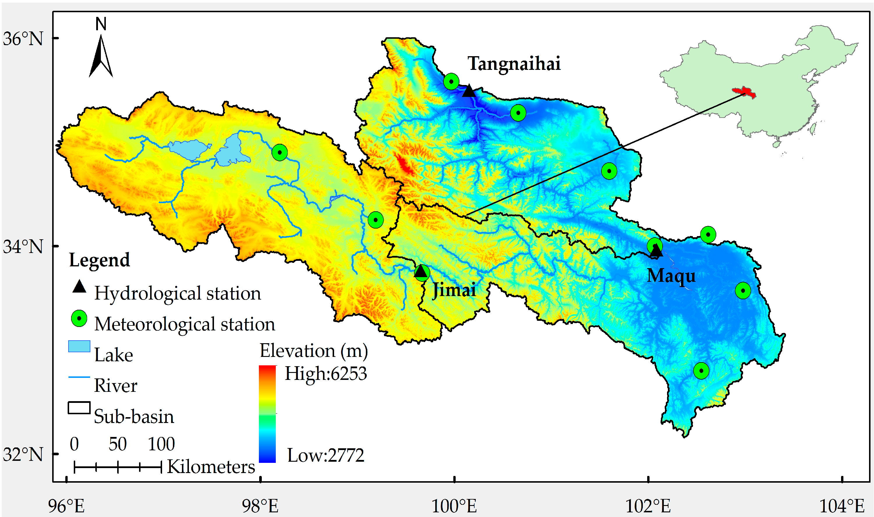
2.1. Study Area

The representative region selected by this study is located in eastern Tibetan Plateau, China, as shown in Figure 1. The geographical location of UYRB is between 32.17°–36°N, 95.8°–103.5°E. The region under study mostly over 4000 m is featured with meandering drainage river crossing the towering mountains and the rolling hills. The UYRB can be divided into three sub-catchments by geography, namely, upstream, midstream, and downstream controlled by Jimai, Maqu and Tangnaihai respectively. The upstream is known as the star-studded lakes including the two largest outflows of freshwater lakes namely Eling Lake and Zaling Lake. The midstream is the main watershed of the UYRB mostly because the marsh wetland consumes lots of space of the midstream which can provide replenishment for the trunk stream. The downstream is characterized by steep-sided river valleys and snowmelt runoff. More information of the three sub-catchments can be achieved from Table 1.
The basin is an alpine climate zone characterized with a dry winter and a rainy summer. In winter, the UYRB is controlled by the Tibetan High which cause a seven-month cold period and most places have no absolute frost-free period. In summer, the UYRB is influenced by the southwest monsoon with thermal low pressure, abundant water vapor and high precipitation accounting for 75–90% of the annual total. In addition, temperature variation of the annual is very small but the temperature variation between day and night is so big. The land use and land cover classes is consisted by the typical Tibet Plateau vegetation belt which is a young derivatives department characterized by high mountain specialization and cold and drought specialization. It consists of evergreen forest, open scrublands, grasslands, and bare ground being the main types. Soil types of the UYRB are dominated by sandy loam, sandy clay and loamy sand being the main types.

2.2. Datasets Description

In the current study, due to restrictions on the availability of the hydrometric stations observations over the UYRB, a twelve-year period from 1 January 2001 to 31 December 2012 has been selected, of which the period from 2001 to 2005 is treated as the calibration period while 2006–2012 is treated as the validation period. Both satellite and gauged precipitation datasets are available in these periods. The historical records of daily datasets are collected from the Chinese Meteorological Administration (CMA) meteorological stations. Moreover, the ground observations including precipitation, minimum temperature, maximum temperature and wind speeds are interpolated into 0.25° × 0.25° grids to match the spatial distribution of satellite precipitation. Besides, daily observed streamflow records of the UYRB are collected from TangNaiHai hydrological station.
This study aimed to assess four SGPEs, namely CRT, BLD, CDR and 3B42 and investigated their suitability in hydrological application over UYRB region. A general introduction description of these products is summarized as follows. The TMA product’s latest version 7 was released in May 2012 by the NASA Goddard Earth Sciences Data and Information Services Center (GES DISC), in which a near real-time version (3B42RT) and a post-real-time version (3B42) are included. These estimates are produced by merging three types of observations such as PMW, IR, and PR from multiple LEO and Geo satellites and ground observations at a spatial resolution of 0.25° × 0.25°, with a temporal resolution of 3-hourly. The main difference is that the TRMM Combined Instrument (TCI) dataset has been used in 3B42 for calibration; however, it was replaced by the TRMM Microwave Imager (TMI) dataset in 3B42RT. Besides, the 3B42 provides the bias-corrected precipitation estimates by inclusion ground gauge observations from the GPCC and the Climate Assessment and Monitoring System (CAMS) at the monthly scale while 3B42RT is a satellite only precipitation estimates. Therefore, the 3B42RT is available approximately nine hours after realtime observations, while the 3B42 is available about 10–15 days after the end of each month. Here, the 3B42 is employed in daily scale from 2001 to 2012.
The CMORPH product stands for the precipitation product estimated by the NOAA Climate Prediction Center MORPHing technique. The latest CMORPH V1.0 products include RAW, CRT and BLD. The CMORPH RAW is a satellite-only precipitation product by combining existing passive microwave-based precipitation estimates from multiple low orbit satellites and the infrared data from multiple geostationary satellites. Based on the RAW product, the CRT product is generated by adopting the probability density function (PDF) matching to conduct bias reduction over land. The CRT product is further combined with the gauge analysis through an optimal interpolation (OI) technique to generate the BLD product. All three products are available at PERSIANN websites [34]. Here, just the two SGPEs versions are applied in daily scale from 2001 to 2012.
The original PERSIANN is one of the popular global precipitation estimation for estimating historical precipitation from March 2000 to present developed by combining IR and PMW observations from GEO and LEO satellite imagery, respectively. The latest CDR uses the archive of the GridSat-B1 IR data as the input to train PERSIANN model; then the biases in the PERSIANN estimated precipitation is adjusted by the Global Precipitation Climatology Project (GPCP) monthly 2.5° product version 2.2. Unlike the other precipitation estimations, the PERSIANN model parameters were pretrained by using the National Centers for Environmental Prediction (NCEP) stage IV hourly precipitation data instead of PMW data. Currently, this version of PERSIANN CDR is only available with high spatial resolution of 0.25° × 0.25° and daily temporal resolution. It can be acquired from 1 January 1983 to present form CMORPH websites [35]. However, in this paper, subset data from 2001 to 2012 are adopted in daily scale.

2.3. Hydrological Model

The hydrologic model used in this study is the Variable Infiltration Capacity (VIC) model which is known as a macroscale and semidistributed land surface hydrologic model. It was first developed by Liang et al. [36,37] for solving both surface water and energy balances over a grid mesh. Then, various updates of the model have been further described, such as cold land process updates [38], snow model updates [39], lakes and wetlands [40]. The key characteristics of the grid-based VIC are the representation of vegetation heterogeneity, multiple soil layers with variable infiltration, and non-linear base flow. The three-layer VIC model (VIC-3L) framework includes a top thin soil layer to represent quick bare soil evaporation following small rainfall events, a middle soil layer to represent the dynamic response of the soil to rainfall events based on the infiltration capacity curve as described by the Xinanjiang hydrological model [41], and a bottom soil layer (third soil layer, maximum depth around 1.5 m) to characterize the seasonal soil moisture behavior based on the drainage in the Arno model [42]. In addition, the simulated streamflow at the basin outlet was post-processed by a separate routing model based on the linearized Saint-Venant equation using the VIC grid results as inputs [43]. Besides, the VIC model assigns many of its parameters based on the vegetation type and soil texture. Although most parameters can be directly estimated from the land surface database, several important parameters including the exponent of variable infiltration capacity curve (B), the maximum velocity of base flow (Dsmax), the fraction of maximum base flow (Ds), the fraction of maximum soil moisture content of the third layer (Ws), the second and the third soil-layer thicknesses (d2 and d3) must be optimized through the model calibration process. For further details, readers can refer to [44]. The VIC model has been widely applied in seasonal hydrological forecasting, climate change impacts studies and water and energy budget studies. Recently, there is a new trend that the VIC model has been popularly used for evaluating the capability of satellite precipitation retrievals in streamflow simulation [21,23,45]. Here, the VIC model will be employed to evaluate the capability of SGPEs in streamflow simulation over UYRB of the TP. To match the resolution of precipitation products from the satellite datasets, the VIC model was set at 0.25° spatial resolution.

2.4. Statistical Evaluation Metrics

To quantitatively analyze the overall performance of SGPEs in comparison with gauged precipitation observations, a set of continuous verification metrics are considered, including correlation coefficient (CC), relative bias (RB), and root mean-square error (RMSE). Also, the CC and RB are operated to assess the performance of simulated streamflow. Besides, the Nash-Sutcliffe (NS) index is carried out to quantify the performance of the hydrological model. The formulas are given as:
C C = i = 1 n ( O b s i O b s ¯ ) ( S i m i S i m ¯ ) i = 1 n ( O b s i O b s ¯ ) 2 i = 1 n ( S i m i S i m ¯ ) 2 ,
R B = i = 1 n ( O b s i S i m i ) i = 1 n S i m i × 100 % ,
R M S E = 1 n i = 1 n ( O b s i S i m i ) 2 ,
N S = 1 i = 1 n ( O b s i S i m i ) 2 i = 1 n ( O b s i O b s ¯ ) 2 ,
where S i m i and O b s i represent SGPE (or simulated streamflow) and ground observed precipitation (or observed streamflow), respectively. S i m ¯ and O b s ¯ are mean values of the corresponding elements.

3. Results and Analysis

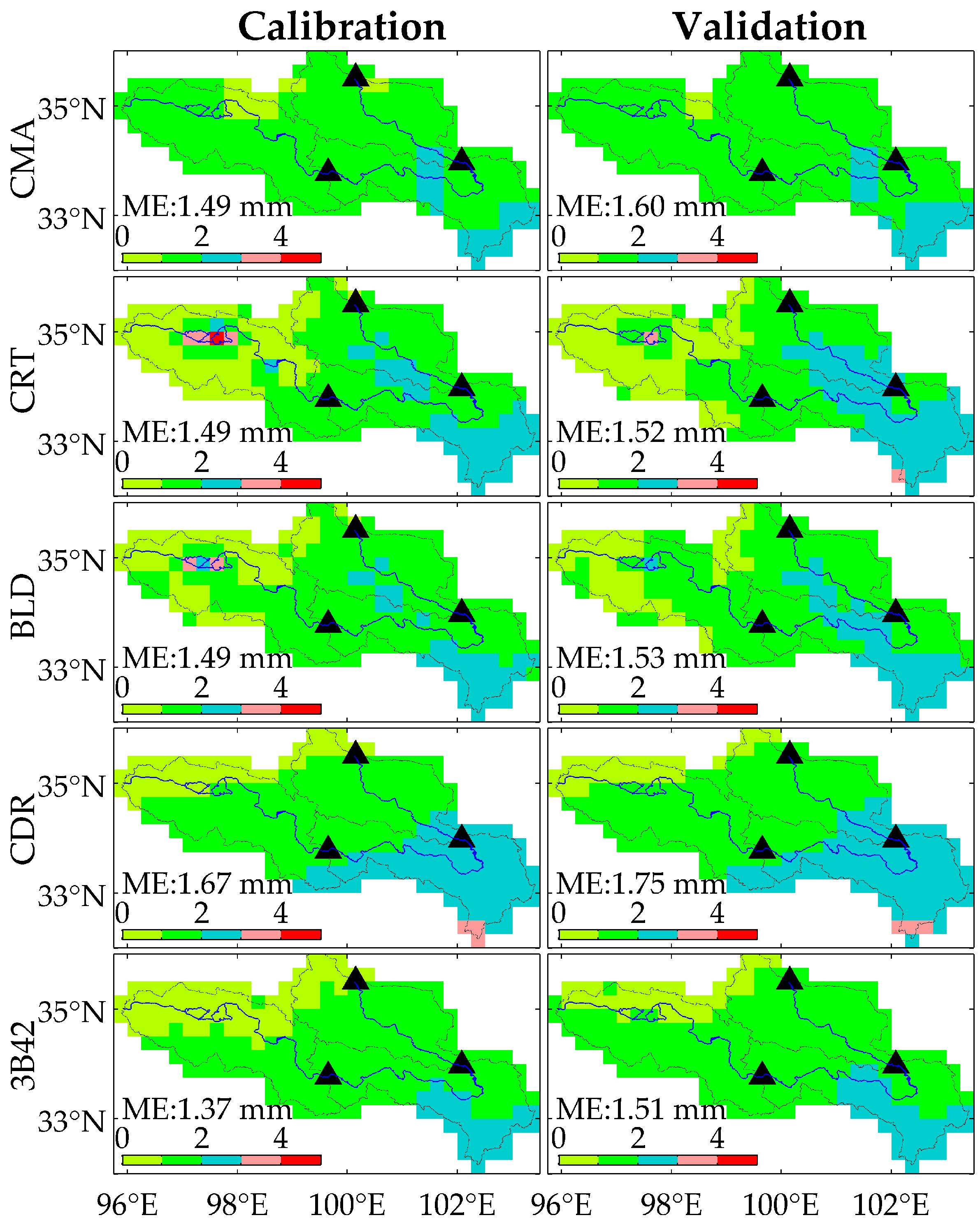
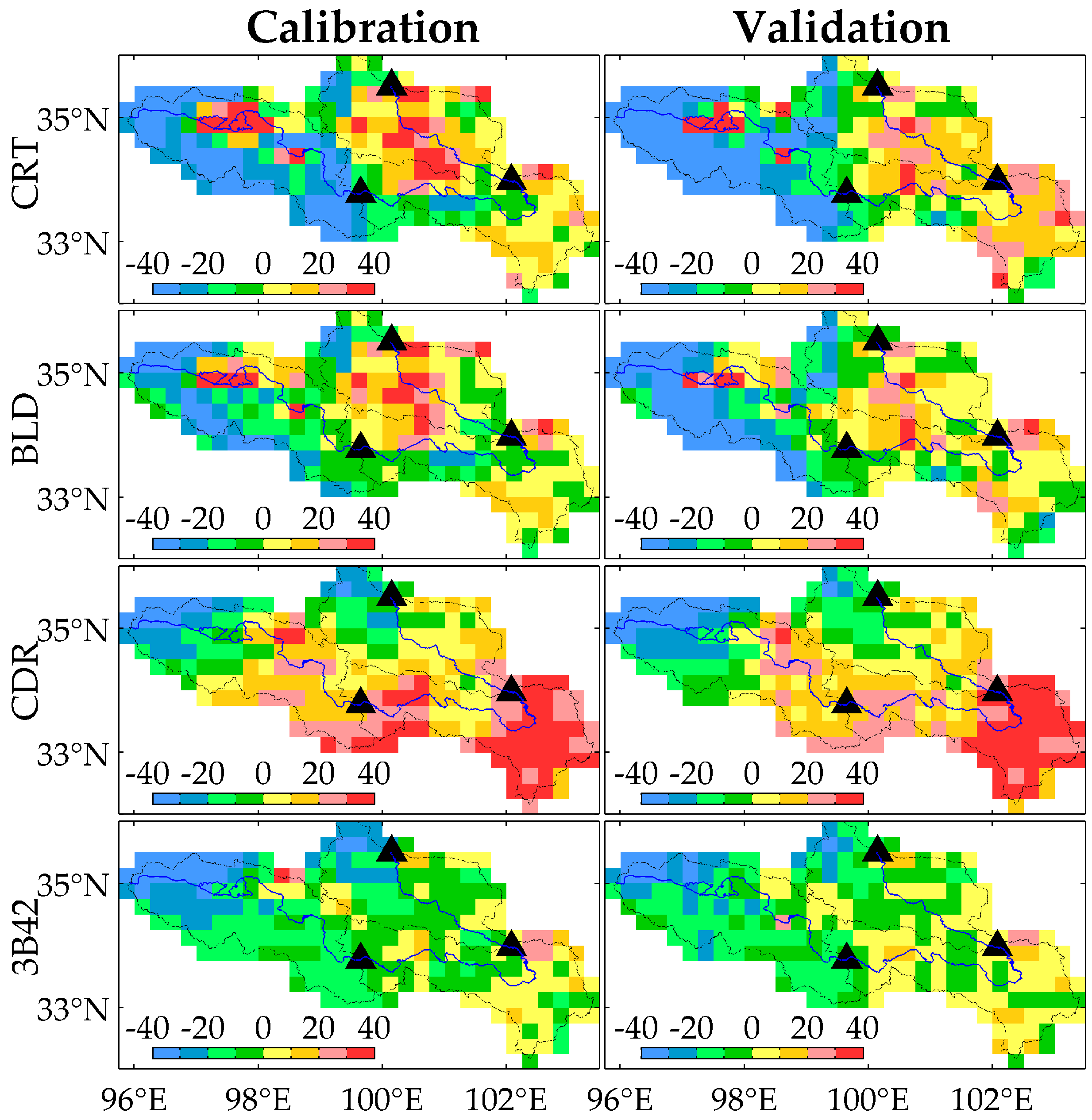
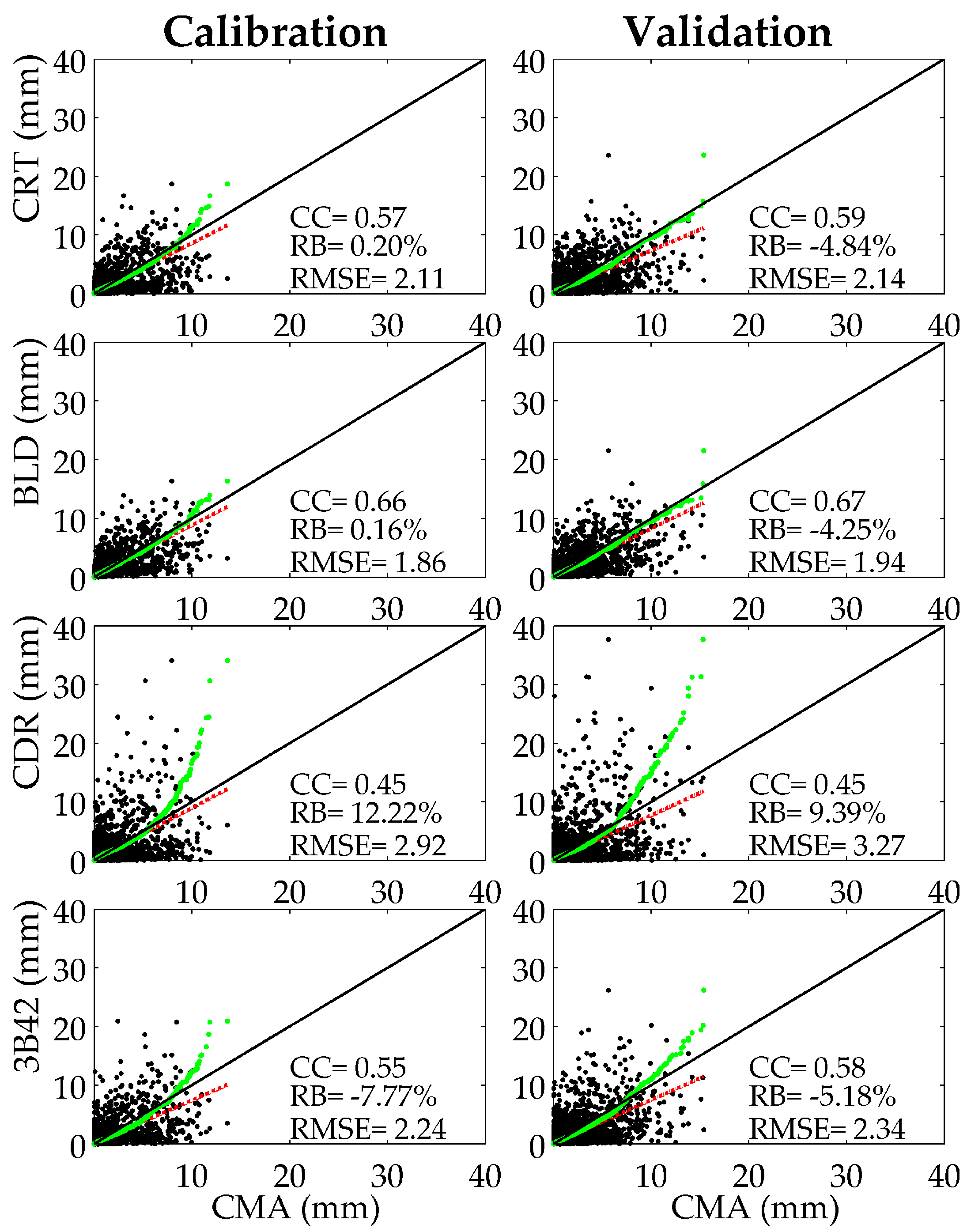
3.1. Evaluation and Comparison of Satellite-Gauged Precipitation Estimates

We evaluated the applicability of the four SGPEs based on CMA over the study region. Because of the negative effects of their associated uncertainties on the hydrological modeling process, the comparative analysis was divided into two periods, which were the calibration (2001–2005) and the validation (2006–2012) periods. This was to investigate and characterize precipitation patterns and error quantification of the four satellite products over the UYRB region. Data in Figure 2 show the spatial distribution of daily average precipitation obtained from CMA and the four SGPEs (CRT, BLD, CDR, and 3B42) tested, respectively for calibration (first column) and validation (second column) periods. Furthermore, the mean values (MEs) of daily average precipitation over the UYRB region had been depicted in Figure 2. Intuitively, Figure 2 shows that the precipitation patterns derived by CMA and the four SGPEs are visually compatible in the two periods with the precipitation intensities gradually decreasing from the eastern part of the basin to the western part. Meanwhile, a large amount of precipitation concentrated upon the southeastern region of the UYRB and the spatial variability analysis revealed that the low-altitude regions of the basin are characterized by higher spatial variability of precipitation in comparison with the high mountainous regions partly due to the abundant moisture supply by the Indian Summer Monsoon from the Bay of Bengal and the orographic enhancement effect in the western part.
It should be noted that the precipitation amount in validation periods was higher than that in the calibration periods. Additionally, both CRT and BLD resembled extremely well with the CMA in precipitation amount. However, some precipitation patches were found in the CRT and BLD estimates in the source region of the UYRB that are not observed in CMA datasets. The primary reason is that CMORPH possesses inherently systematic anomalies over inland water bodies [46]. However, these systematic anomalies in validation period were slighter than those in calibration period. Furthermore, compared to CMA datasets, CDR had the highest precipitation estimates in both periods while 3B42 reaches the lowest value.
The RB of the SGPEs against the CMA data in both calibration and validation periods are shown in Figure 3. In general, the four SGPEs showed an underestimation of the precipitation in the upstream regions dominated by mountains and an overestimation in the midstream and downstream regions with low-altitude during the two periods. Regardless of the overestimation over the area of Zhaling Lake and Eling Lake, CRT exhibited an obvious pattern that the negative biases primarily occurred in the western region of east longitude 99° while the positive biases are located in the eastern region during the calibration period and these underestimation and overestimation become more visible in validation period. Compared with the corresponding datasets, CRT, BLD exhibited a similar spatial pattern of RB with more petty negative and positive biases, respectively in the west and the east. This means that BLD is more close to CMA than CRT in precipitation amount. Concurrently, CDR showed a large positive bias in the southeast UYRB and the regions close to Jimai hydrological station while slight negative bias just occured in source region and outlet region of UYRB region. Correspondingly, 3B42 underestimateds the precipitation in source region and outlet region of UYRB but there was no prominent overestimation in the southeast UYRB and the regions close to Jimai hydrological station during the two periods.
To check the consistency of precipitation in time series, the basin averaged precipitation from SGPEs versus CMA datasets were scattered in Figure 4 respectively. Meanwhile, the Quantile-Quantile (Q-Q) plot technique was adopted to illustrate more insight into the nature of the differences between the four satellites and the CMA data in both calibration (2001–2005) and validation (2006–2012) periods over the UYRB region. It is well known that if the SGPEs are close to the observed ones, the points in the Q-Q plots should fall close to the 45° reference line. The greater the departure from the reference line or the nonlinearity of the resulting graph is, the greater the evidence of heterogeneity is [47]. It was evident that BLD has the best consistency with CMA in both calibration and validation periods. Simultaneously, the differences in daily average precipitation estimates between SGPEs and CMA became more distinct as the precipitation amount increased. Furthermore, the performance exhibited by CRT was similar to 3B42 in the two periods while CDR tends to overestimate precipitation in both calibration and validation periods.
In addition, the three statistical indexes including CC, RB and RMSE were calculated based on CMA data in two periods as shown in Figure 4. Generally, the best values of CC = 0.66 and CC = 0.67 from BLD were found in calibration period and validation period, respectively. Also, BLD had the best RB and RMSE displayed as 0.16%, −4.25% and 1.86, 1.94 during the two periods, respectively. In contrast, CDR showed the poorest values with CC = 0.45, RB = 12.22% and RMSE = 2.92 in calibration period and CC = 0.45, RB = 9.39% and RMSE = 3.27 in validation period. Moreover, the three statistical standards of CRT were very close to that of 3B42 in validation period. The values of CC and RMSE from CRT were approximately equal to those from 3B42 in validation period, but 3B42 tended to underestimate the precipitation amount in calibration period and there is no evidence to support this phenomenon in CRT with RB = 0.2%.

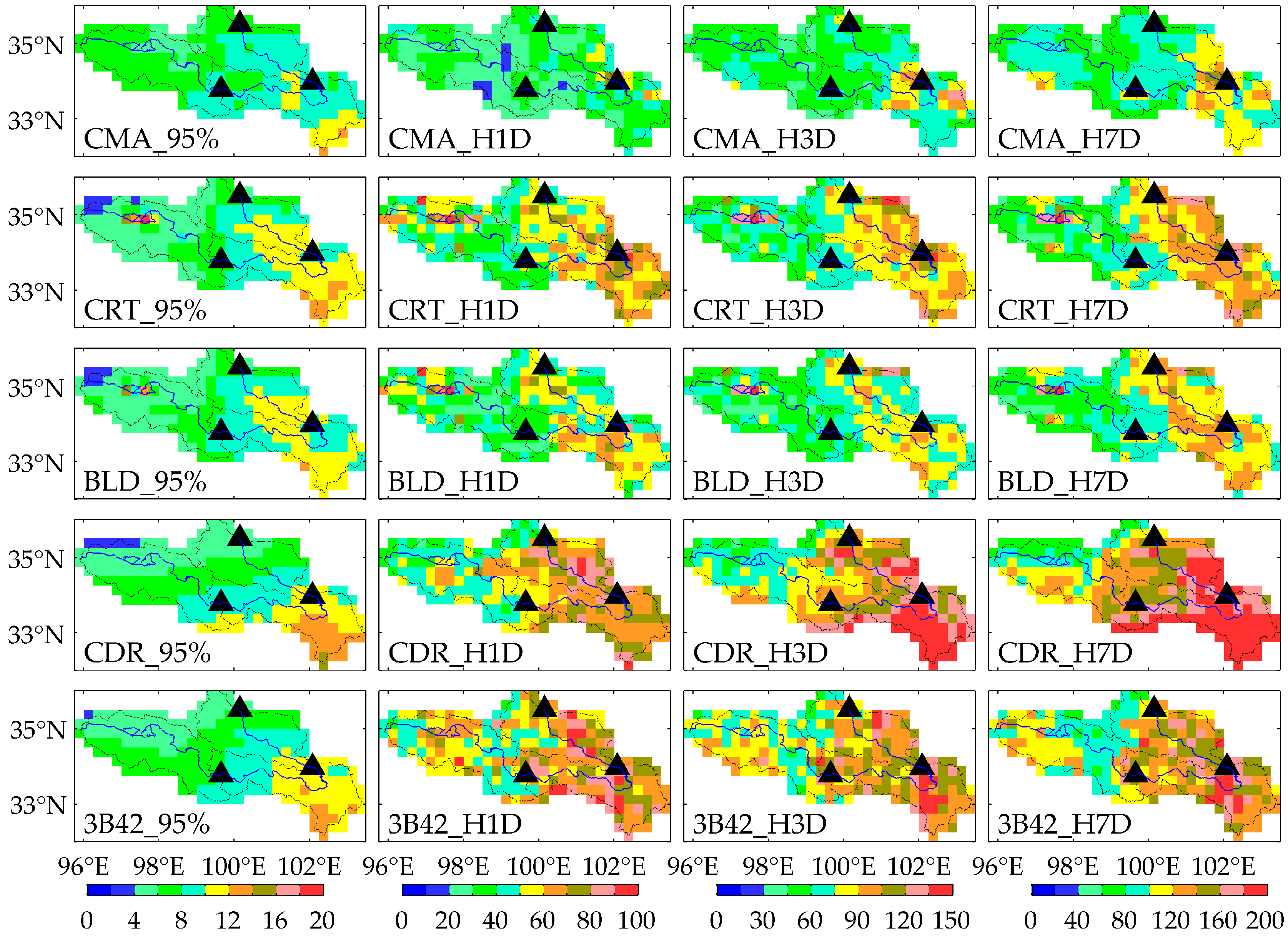
3.2. Extreme Precipitation Analysis

To reveal the changing features of extreme precipitation in the UYRB region, four extreme precipitation scenarios were chosen according to Jiang et al. [9], which are the 95th percentile of daily precipitation (95% pr), the maximum 1-day precipitation (H1D pr), the maximum 3-day precipitation total precipitation (H3D pr) and the maximum 7-day total precipitation (H7D pr) for each pixel during 2001–2012. Difference of the SGPEs from the four extreme precipitation scenarios were compared in Figure 5 respectively. The spatial pattern of the 95% pr from CMA and SGPEs were similar to that of the corresponding daily average precipitation illustrated in Figure 2. It can be observed that the value of 95% pr is large higher than that of the daily average precipitation. From the 95% pr analysis, it was found that the spatial heterogeneity of CMA was slightest probably because of the influence of interpolation. In contrast, CDR had the strongest spatial heterogeneity over 15 mm/day in southeast corner and under 3 mm/day in northwest corner. The difference in spatial heterogeneity between CDR and CMA was gradually growing in the scenario of H1D, H3D and H7D. For the scenario of H7D, nearly half of the UYRB had more than 200 mm precipitation in seven days but most regions in CMA was lower than 100 mm in seven days. Besides, 3B42 had much higher value than CMA in the western UYRB in terms of the four extreme cases of 95%, H1D, H3D and H7D. This differed from the daily average case when 3B42 underestimated the precipitation amount. Without the consideration of the overestimation over inland water bodies, both CRT and BLD enjoyed the similar spatial distribution and precipitation amount estimation to CMA for the four extreme cases, although they overestimate the precipitation amount in the western basin. In general, the extreme precipitation variability varies greatly over the UYRB. The high values were mainly concentrated in the middle basin while less extreme higher precipitation occurred in downstream reaches and the least extreme higher precipitation was found in the source region. Although the four satellite estimates were all overestimated the extreme precipitation amount over western region, compared with CDR and 3B42, both the spatial distribution and the precipitation amount of CRT and BLD were better agreement with the real extreme precipitation in CMA.

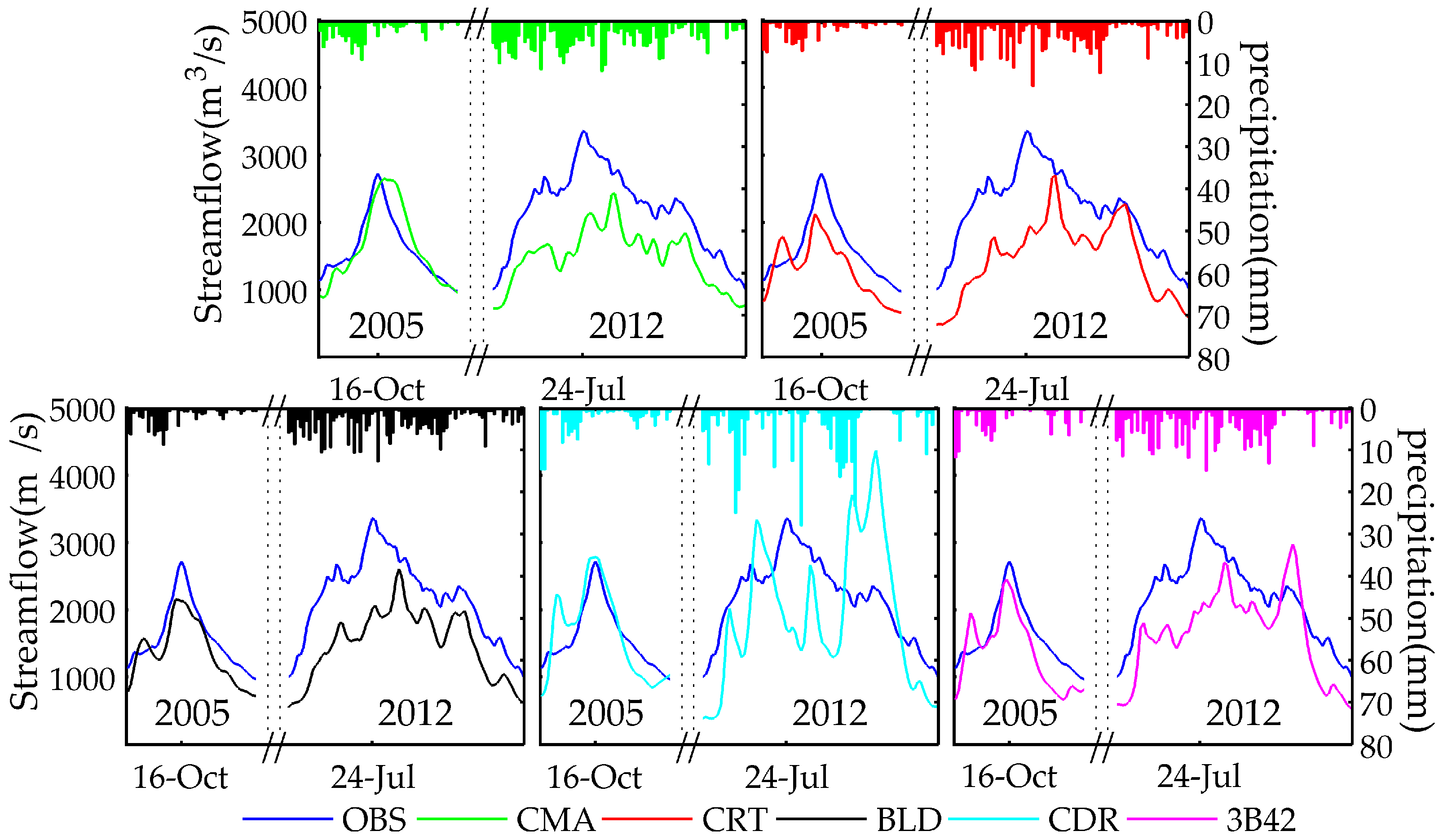
3.3. Streamflow Simulations Analysis

Here, the VIC model was firstly calibrated by comparing the observed and simulated streamflow forced by the CMA precipitation data in the calibration period over the UYRB. The parameters subjected in calibration and the sensitivity of those parameters were discussed in detail in [48]. Subsequently, the period 2006–2012 was used for model validation. Lastly, the VIC model was forced by CRT, BLD, CDR and 3B42 as inputs for twelve years (2001–2012) with the model parameters calibrated using CMA data in the calibration period. The comparison of simulated streamflow and observed streamflow in both calibration and validation period are illustrated in Figure 6. It can be seen that the simulated streamflow hydrograph can reasonably well match the observed streamflow, especially for the high peak discharges in wet seasons. In spite of the overestimation in the dry seasons, the performance of the VIC model did not affect subsequent analysis associated with the relatively low discharges in the dry seasons. Besides, the three statistical indicators for calibration, verification and the whole periods are listed in Table 2, respectively. Overall, the VIC model was capable of capturing the timing and magnitude of the daily observed streamflow.
The calibrated VIC model was then used to evaluate the SGPEs in streamflow simulation over the UYRB, without any further adjustment of parameters. Keeping the same parameters allows us to investigate how differences of SGPEs affect the accuracy or quality of VIC streamflow simulation. Figure 7 shows the daily simulated streamflow with the precipitation forcing from the four SGPEs over the UYRB. Intuitively, the SGPEs driven simulations catch the fluctuation of daily hydrograph well, although underestimated/overestimated of peak floods existed in some cases. However, compared to Figure 6, none of the four SGPEs driven simulations made significant contributions to improve the performance of streamflow simulation in the timing and magnitude of the observed streamflow. In fact, given that the model was calibrated with CMA, that is not surprising. Besides, the streamflow simulation forced by CDR overestimated the flood peak in both the calibration and verification periods, which was probably because CDR overestimated the amount of precipitation in midstream. The BLD simulation showed the best consistent with the observed daily hydrograph, but it tends to overestimated the peak in calibration period (except for 2005) and underestimated the peak in validation period (except for 2006). The overvalued or undervalued scenarios were more noticeable in CRT simulation results. Moreover, excepting 2001 and 2010, the 3B42 simulations chould capture the peak very well but there was a large fluctuation in the 3B42 simulations with the snipy peak. In addition, the statistic summary of the comparison between the observed and the SGPEs forced scenarios also be shown in Table 2. The simulation results of hydrological model were directly depend on precipitation input, the more accurate the precipitation input, the better the simulation results. Overall, from Table 2, the CMA simulations have showed the best performance of all, followed by BLD. Duo to the overestimation in heavy rain, CDR simulation scenario overrates the flood peaks in in wet seasons and showed poor NS indicators. As for 3B42 simulation scenario, it had the best values of RB (3.84%, −6.64% and −2.75% respectively) although the NS of 3B42 (0.62, 0.65 and 0.64 respectively) were lower than that of CMA (0.80, 0.80 and 0.81 respectively). CRT simulation scenario exhibited a large overestimation in hydrograph over calibration period, but it showed a similar performance of 3B42 simulations in verification period.

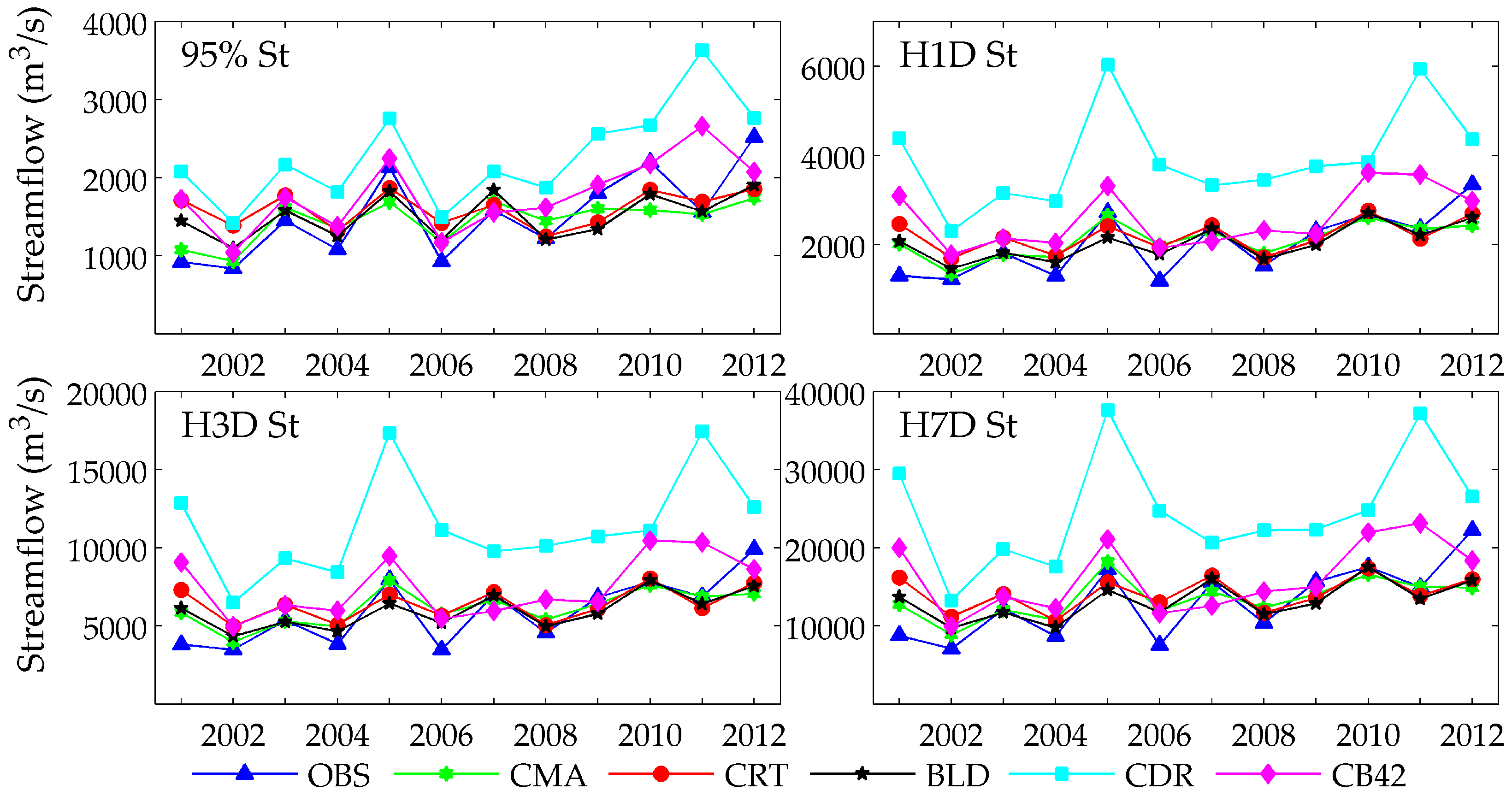
3.4. Extreme Streamflow Analysis

Figure 8 shows the extreme values of observed streamflow and simulated streamflow driven by CMA and SGPEs in the UYRB from 2001 to 2012. The four extreme streamflow scenarios illustrated in Figure 8 were the 95th percentile of daily streamflow, the maximum 1-day streamflow (H1D St), the maximum 3-day streamflow (H3D St) and the maximum 7-day streamflow (H7D St) for each year of study period respectively. The results showed that the CMA could capture the main patterns of the extreme streamflow in the UYRB by using VIC hydrological model with slight underestimation in flood years and hidden overestimation in dry years. CRT and BLD exhibited comparable hydrologic performance to CMA, especially for BLD in HID St, H3D St and H7D St scenarios. 3B42 also captured the main patterns of the extreme streamflow. However, excepting 2007 and 2012, it had an explicit overestimation in the four scenarios. Similar case occurred in CDR forced scenario, it captured the main patterns of the extreme streamflow but enjoyed the largest overestimation. Besides, the statistic summary of the comparison between the observed and simulated extreme streamflow is shown in Table 3.
Based on the works reported in [49], it was found that floods in UYRB are characterized by rise and fall flat, long duration, low peak and huge flood volume. The capability of satellite-based products in predicting severe flood events was evaluated. In July and August 2012, there was a long and continuous duration heavy rainfall occurred over UYRB. The everlasting torrential rain had led to the most serious flood in UYRB since 1989 [49]. The largest discharge of the 2012 flood event was 3350 m3/s occurring on 24 July 2012. Besides, a high discharge of 2720 m3/s is found on 6 October 2005. These two floods have brought great flood control pressure to the deployment of the longyangxia reservoir downstream. The statistical characteristics of the two floods have been shown in Table 4.
The observed streamflows and simulated streamflows forced by CMA and four SGPEs are illustrated in Figure 9. As the simulation hydrographs are cohesive sets of the corresponding precipitation input, the time series of precipitation during the flood events are also plotted in Figure 9. In addition, the three statistical indicators (RB, CC and RMSE) for SGPEs against CMA data during the flood period over UYRB have been analyzed in Figure 10. Owing to the perfect match in magnitude and timing of the event 2005 flood, CMA is further believed to reflect the spatial and temporal distribution of precipitation during the 2005 flood. Compared to CMA, CRT and BLD both enjoy a negative RB during the event 2005 flood, but BLD had a higher CC and a lower RMSE than CRT. Hence, BLD forced simulation scenario showed a better performance than that of CRT in 2005 flood period in spite of the underestimation in flood peak. Combinative comparison of Figure 9 and Figure 10 showed that CDR possessed a positive RB but the CDR forced simulation scenario matches the flood peak best in the 2005 flood period. This illustrates that CDR had great uncertainty in space-time distribution and the median and the mean values should not be used exclusively as measures of location when there are evident outliers. Moreover, the lower flood peaks were found in SGPEs based simulation results but not found in observed streamflow and CMA forced scenario, which is mainly because of the unreliable antecedent precipitation in SGPEs.
Unfortunately, the CMA based simulation results significantly underestimated the flood events of 2012, and the CMA based flood peak lags behind the observed values. This indicates that the veracity of the CMA based precipitation is questionable in amount and occurrence time in the 2012 flood period. So the quantitative assessment using CMA as the reference is unreliable over the 2012 flood period. However, the accurate spatial and temporal precipitation distribution plays an important role in generating realistic streamflow through distributed hydrologic models. The performance of precipitation can be indirectly analyzed from the simulation results. Three major flood peaks continuously happened on 12 July, 24 July and 24 August, and the middle flood event was the heaviest. Although CRT accurately captured the magnitude and time of the third flood peak, but CRT and BLD forced simulations greatly underestimate the previous two flood peaks. Low quality in reproducing 2012 flood event reflects once again that both CRT and BLD is incompetent in detecting extreme precipitation during the flood 2012 event. For 3B42, it was observed that there exist remarkable magnitude differences with underrating the first two peaks and overrating the third one, and there was a time delay for middle flood. These observation show that 3B42 underestimated the inchoate precipitation but overestimated the later precipitation during the 2012 flood period. CDR forced hydrograph missed the flood peak and had large jumps which is mainly because of that CDR better depicted the total areal rainfall but misrepresented the heavy precipitation’s pattern and occurred time.

4. Discussion

By merging ground-based observations, SGPEs could reduce the errors of SPEs and showed a new opportunity for basin-scale hydrological applications. However, the adjusted/merged procedures in the production of SGPEs greatly affected their quality of precipitation estimation. Despite the adjustment by GPCP monthly precipitation, the CDR product with the IR data as the input to PERSIANN model showed an intrinsic deficiency over UYRB. Given the longer time series (1983 to present), the CDR product is still extremely valuable in investigating climate change with high resolution. As for the two CMORPH-based SGPEs, benefiting from the two step bias correction method (PDF-OI merging algorithm), BLD showed more stable performances than CRT whose overall quality was comparable with 3B42. Since CRT use PDF matching to adjust daily bias of CMORPH RAW data while 3B42 only handles the monthly biases, on the other hand, the OI procedure used in BLD is considered to be a more effective method in improving precipitation estimates. However, further evaluations in extreme precipitation analysis indicated that the CRT showed great advantage over 3B42, which showed the fine time-scale modifications can better capture wickedly heavy precipitation.
For streamflow simulating, the hydrological utility of SGPEs was associated with large uncertainties form parameters and model structures. Theoretically, the parameters of hydrological model should be calibrated using the “perfect” observed precipitation data in a dense gauge network, so that they can be the best possible approximation of watershed hydrological features. Nevertheless, restricted to the high altitude, the gauge network’s distribution over UYRB is sparse. A few studies [33] suggested that recalibrated the hydrological model using the SGPEs can greatly improve the streamflow simulation performance. The uncertainty of parameters and the comparison of different models are being carried out in the following research. Moreover, since hydrological processes in distributed hydrologic models were sensitive to the total precipitation amount as well as rainfall intensity distribution, the errors of SGPEs were also propagated into hydrologic simulations. Using the parameters calibrated with CMA, the general streamflow pattern forced by the four SGPEs exhibits fair agreement with observation. Note that CRT and BLD were remarkably superior to 3B42 and CDR in flood peak simulation, this indicates again the superiority of fine time-scale correction. However, in the streamflow simulations analysis especially for the two flood events, the simulation results forced by the four SGPEs are not satisfactory. This is mostly because the rain gauge observations used in SGPEs are limited to GTS reports and it is hard to capture heavy rain center effectively through sparse gauge network. Despite of the same PDF-OI merging algorithm, the work in [31] indicated that the newly developed SGPE which combines the CMORPH RAW data with daily precipitation observations from about 2400 gauges in China had a better performance than BLD over Huaihe river basin. With more available rain gauge observations, there are great advantages of regional or national scale modifications in improving the quality of precipitation data. Besides, the meteorological stations over UYRB region are mainly located in the midstream and downstream regions, more efforts are therefore urgently needed to build a denser rain gauge observation network in the upstream regions where are characterized by complex terrain and a rigid climate.

5. Summary and Conclusions

In this paper, we have made a comprehensive analysis of the applicability and reliability of the latest SGPEs (CRT, BLD, CDR, and 3B42) against gauge-based datasets (CMA) in UYRB where it is a most important watershed of the TP during January 2001–December 2012. Subsequently, their utility in streamflow prediction was compared by driving VIC model. Last, the changes of extreme precipitation and extreme streamflow were analyzed.
The main results are summarized as follows:
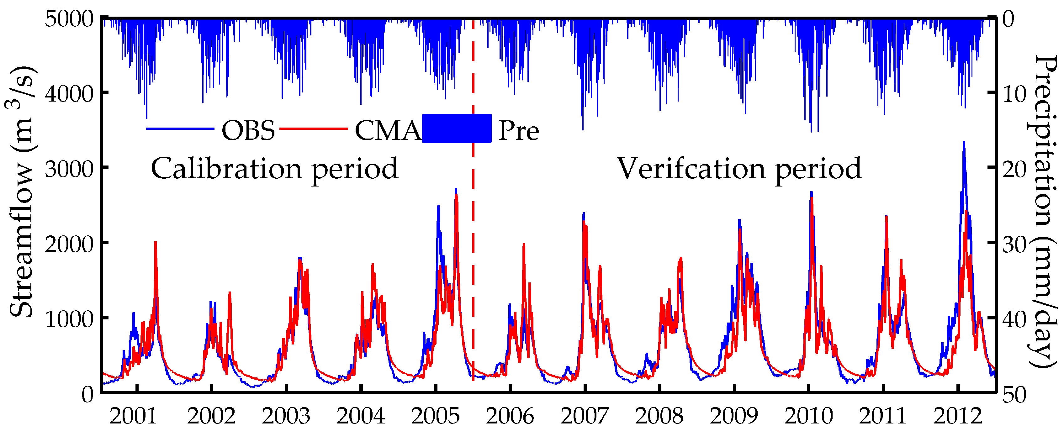
  • Compared to the CMA precipitation, the four SGPEs could generally captured the spatial distribution of precipitation well in spite of the underestimation in the western mountains and overestimation in the southeast which is located in a lower elevation. Overall, CDR overrated the precipitation in basin scale while 3B42 performs best. However, the two CMORPH (CRT and BLD) agreed well with CMA in time series of watershed average precipitation in both the calibration and verification periods.
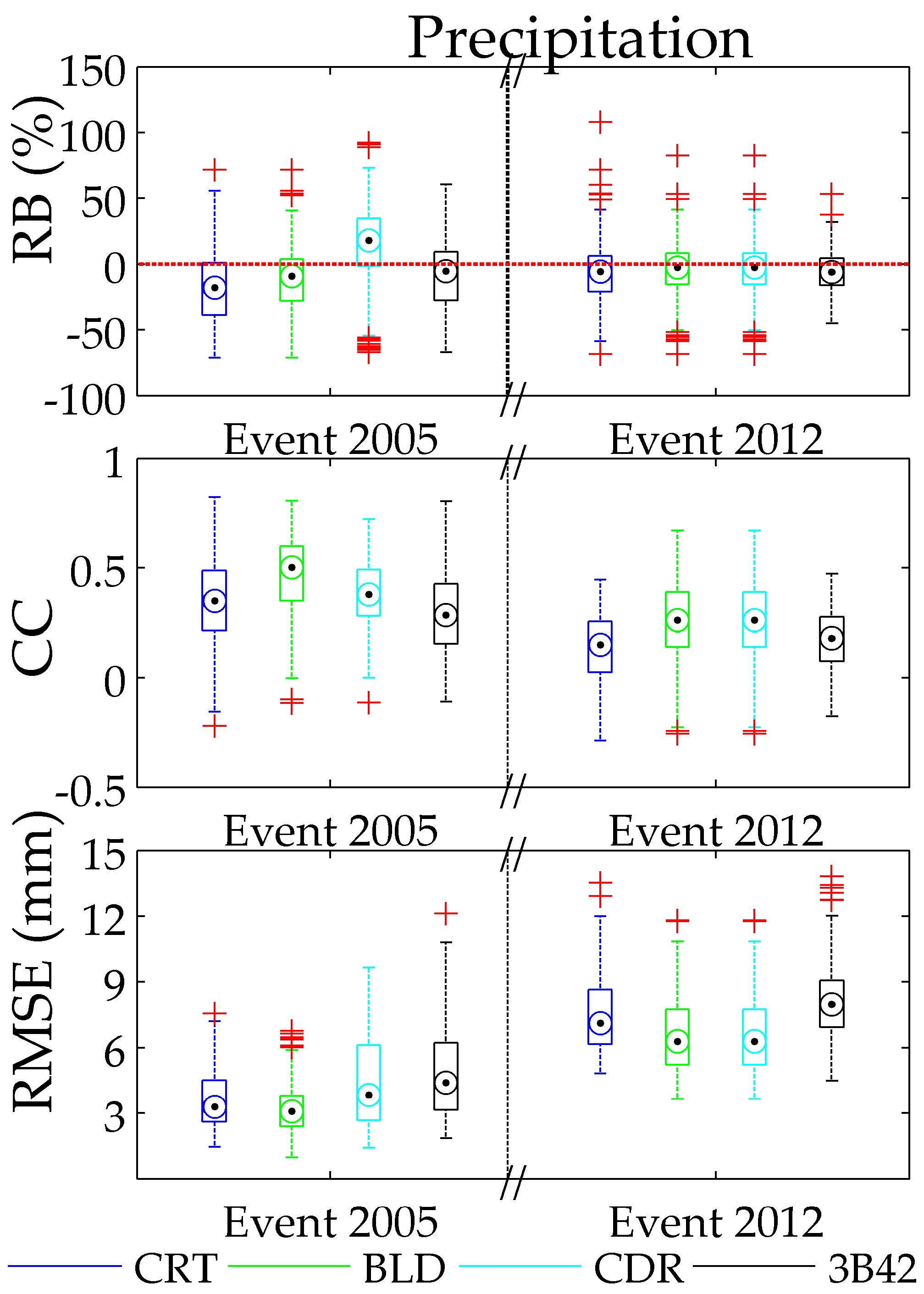
  • The spatial pattern of the extreme precipitation was similar to that of daily average precipitation with the precipitation amount increasing from the northwest to the southeast. The disastrous heavy rain mainly occurred in the southeast corner of the basin. Also, 3B42 and CDR overestimated the extreme precipitation, especially in the southeast, while CRT and BLD were closer to CMA in the distribution of extreme precipitation.
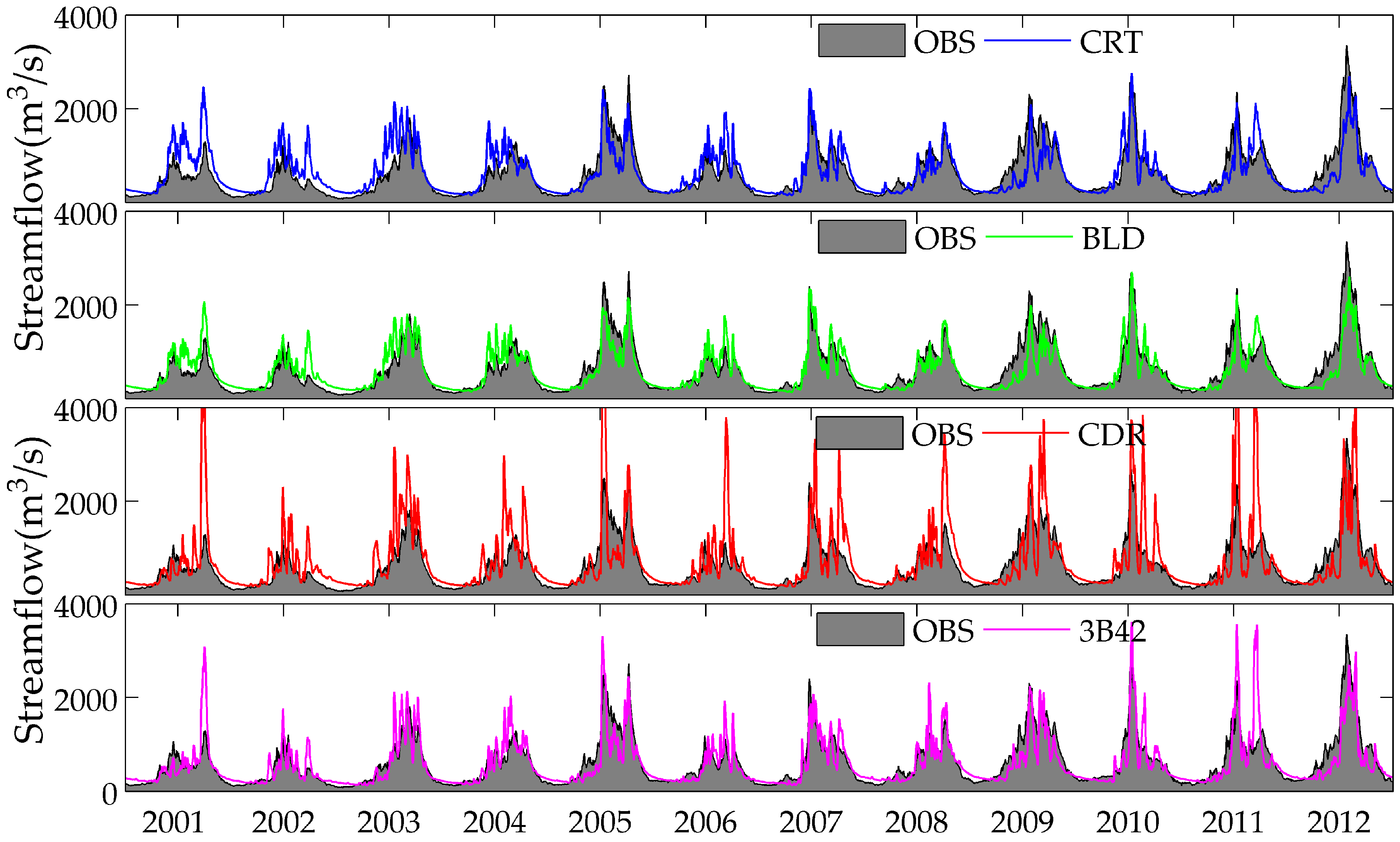
  • Notice that none of the four SGPEs performed better than CMA in hydrologic utility. However, BLD performed fairly well and showed comparable hydrologic utility with CMA over UYRB, and CRT and 3B42 showed an acceptable performance. In contrast, CDR is equipped with little potential for the streamflow simulation with wildly overrating the discharge in flood season. This is closely related to the overreaction of the extreme precipitation over the southeastern part of UYRB.
  • It can be seen that the four SGPEs showed well performance in the 2005 floods event, while they all exhibited poor performance in matching the hydrograph of the 2012 flood event which was a disastrous flood for the longyangxia reservoir. The simulation results of 2012 flood event indicated that maybe there exist large errors in SGPEs for a few rather large torrential rain events which could generate errors in estimating flood peaks, peak times and flood volume. Hence, it should be used with caution for the SGPEs in simulating massive flood events over UYRB.

Acknowledgments

The authors wish to acknowledge the reviewers of the manuscript for their constructive comments and helpful suggestions. This research is supported by National Key Research and Development Program (grant number: 2016YFC0400909, 2016YFA0601504); NNSF (grant numbers: 41371049, 41571015, 41323001, and 51539003); and the Project of the State Key Laboratory of Hydrology-Water Resources and Hydraulic Engineering, China (grant number: 20165042612).

Author Contributions

All authors contributed extensively to the work presented in this paper. Haishen Lu and Yonghua Zhu designed the framework of this study. Jianbin Su analyzed the data and wrote the paper. Haishen Lu and Yonghua Zhu revised the paper. Jianqun Wang and Ali M. Sadeghi helped check the English language and style.

Conflicts of Interest

The authors declare no conflict of interest.

References

  1. Hong, Y.; Adler, R.F.; Huffman, G.J.; Pierce, H. Applications of Trmm-Based Multi-Satellite Precipitation Estimation for Global Runoff Prediction: Prototyping a Global Flood Modeling System; Springer: Dordrecht, The Netherlands, 2010; pp. 245–265. [Google Scholar]
  2. Winsemius, H.C.; Aerts, J.; van Beek, L.P.; Bierkens, M.F.; Bouwman, A.; Jongman, B.; Kwadijk, J.C.; Ligtvoet, W.; Lucas, P.L.; van Vuuren, D.P. Global drivers of future river flood risk. Nat. Clim. Chang. 2016, 6, 381–385. [Google Scholar] [CrossRef]
  3. Rozalis, S.; Morin, E.; Yair, Y.; Price, C. Flash flood prediction using an uncalibrated hydrological model and radar rainfall data in a mediterranean watershed under changing hydrological conditions. J. Hydrol. 2010, 394, 245–255. [Google Scholar] [CrossRef]
  4. Sorooshian, S.; Hsu, K.L.; Coppola, E.; Tomassetti, B.; Verdecchia, M.; Visconti, G. Hydrological Modelling and the Water Cycle; Springer: New York, NY, USA, 2008. [Google Scholar]
  5. Meng, J.; Li, L.; Hao, Z.; Wang, J.; Shao, Q. Suitability of trmm satellite rainfall in driving a distributed hydrological model in the source region of yellow river. J. Hydrol. 2014, 509, 320–332. [Google Scholar] [CrossRef]
  6. Yong, B.; Ren, L.L.; Hong, Y.; Wang, J.H.; Gourley, J.J.; Jiang, S.H.; Chen, X.; Wang, W. Hydrologic evaluation of multisatellite precipitation analysis standard precipitation products in basins beyond its inclined latitude band: A case study in Laohahe basin, China. Water Resour. Res. 2010, 46, 759–768. [Google Scholar] [CrossRef]
  7. Mishra, A.K.; Coulibaly, P. Developments in hydrometric network design: A review. Rev. Geophys. 2009, 47, 2415–2440. [Google Scholar] [CrossRef]
  8. Huffman, G.J.; Adler, R.F.; Morrissey, M.M.; Bolvin, D.T.; Curtis, S.; Joyce, R.; Mcgavock, B.; Susskind, J. Global precipitation at one-degree daily resolution from multisatellite observations. J. Hydrometeorol. 2001, 2, 36–50. [Google Scholar] [CrossRef]
  9. Jiang, S.; Zhang, Z.; Huang, Y.; Chen, X.; Chen, S. Evaluating the trmm multisatellite precipitation analysis for extreme precipitation and streamflow in ganjiang river basin, China. Adv. Meteorol. 2017, 2017, 177–195. [Google Scholar] [CrossRef]
  10. Huffman, G.J.; Bolvin, D.; Nelkin, E.; Wolff, D.B.; Adler, R.F.; Gu, G.; Hong, Y.; Bowman, K.P.; Stocker, E.F. The trmm multisatellite precipitation analysis (tmpa): Quasi-global, multiyear, combined-sensor precipitation estimates at fine scales. J. Hydrometeorol. 2007, 8, 38–55. [Google Scholar] [CrossRef]
  11. Joyce, R.J.; Janowiak, J.E.; Arkin, P.A.; Xie, P. Cmorph: A method that produces global precipitation estimates from passive microwave and infrared data at high spatial and temporal resolution. J. Hydrometeorol. 2004, 5, 487–503. [Google Scholar] [CrossRef]
  12. Sorooshian, S.; Hsu, K.L.; Gao, X.; Gupta, H.V.; Imam, B.; Dan, B. Evaluation of persiann system satellite–based estimates of tropical rainfall. Bull. Am. Meteorol. Soc. 2010, 81, 2035–2046. [Google Scholar] [CrossRef]
  13. Xue, X.; Hong, Y.; Limaye, A.S.; Gourley, J.J.; Huffman, G.J.; Khan, S.I.; Dorji, C.; Chen, S. Statistical and hydrological evaluation of trmm-based multi-satellite precipitation analysis over the wangchu basin of bhutan: Are the latest satellite precipitation products 3b42v7 ready for use in ungauged basins? J. Hydrol. 2013, 499, 91–99. [Google Scholar] [CrossRef]
  14. Ebert, E.E.; Janowiak, J.E.; Kidd, C. Comparison of near-real-time precipitation estimates from satellite observations and numerical models. Bull. Am. Meteorol. Soc. 2010, 88, 47. [Google Scholar] [CrossRef]
  15. Gebregiorgis, A.S.; Tian, Y.; Peters-Lidard, C.D.; Hossain, F. Tracing hydrologic model simulation error as a function of satellite rainfall estimation bias components and land use and land cover conditions. Water Resour. Res. 2012, 48, 11509. [Google Scholar] [CrossRef]
  16. Gebremichael, M.; Bitew, M.M.; Hirpa, F.A.; Tesfay, G.N. Accuracy of satellite rainfall estimates in the blue nile basin: Lowland plain versus highland mountain. Water Resour. Res. 2015, 50, 8775–8790. [Google Scholar] [CrossRef]
  17. Mei, Y.; Nikolopoulos, E.I.; Anagnostou, E.N.; Borga, M. Evaluating satellite precipitation error propagation in runoff simulations of mountainous basins. J. Hydrometeorol. 2015, 17. [Google Scholar] [CrossRef]
  18. Gao, Y.; Liu, M. Evaluation of high-resolution satellite precipitation products using rain gauge observations over the Tibetan plateau. Hydrol. Earth Syst. Sci. 2013, 17, 837–849. [Google Scholar] [CrossRef]
  19. Jiang, S.H.; Zhou, M.; Ren, L.L.; Cheng, X.R.; Zhang, P.J. Evaluation of latest tmpa and cmorph satellite precipitation products for Yellow river basin. Water Sci. Eng. 2016, 9, 87–96. [Google Scholar] [CrossRef]
  20. Li, Z.; Yang, D.; Hong, Y. Multi-scale evaluation of high-resolution multi-sensor blended global precipitation products over the Yangtze river. J. Hydrol. 2013, 500, 157–169. [Google Scholar] [CrossRef]
  21. Tong, K.; Su, F.; Yang, D.; Hao, Z. Evaluation of satellite precipitation retrievals and their potential utilities in hydrologic modeling over the tibetan plateau. J. Hydrol. 2014, 519, 423–437. [Google Scholar]
  22. Alazzy, A.A.; Lü, H.; Chen, R.; Ali, A.B.; Zhu, Y.; Su, J. Evaluation of satellite precipitation products and their potential influence on hydrological modeling over the Ganzi river basin of the Tibetan plateau. Adv. Meteorol. 2017. [Google Scholar] [CrossRef]
  23. Siddiqueeakbor, A.H.M.; Hossain, F.; Sikder, S.; Shum, C.K.; Tseng, S.; Yi, Y.; Turk, F.J.; Limaye, A. Satellite precipitation data-driven hydrological modeling for water resources management in the ganges, brahmaputra, and meghna basins. Earth Interact. 2014, 18, 1–25. [Google Scholar] [CrossRef]
  24. Wang, S.; Liu, S.; Mo, X.; Peng, B.; Qiu, J.; Li, M.; Liu, C.; Wang, Z.; Bauergottwein, P. Evaluation of remotely sensed precipitation and its performance for streamflow simulations in basins of the southeast Tibetan plateau. J. Hydrometeorol. 2015, 16, 342–354. [Google Scholar] [CrossRef]
  25. Wang, W.; Lu, H.; Yang, D.; Sothea, K.; Jiao, Y.; Gao, B.; Peng, X.; Pang, Z. Modelling hydrologic processes in the mekong river basin using a distributed model driven by satellite precipitation and rain gauge observations. PLoS ONE 2016, 11. [Google Scholar] [CrossRef] [PubMed]
  26. Chen, M.; Shi, W.; Xie, P.; Silva, V.B.S.; Kousky, V.E.; Wayne Higgins, R.; Janowiak, J.E. Assessing objective techniques for gauge-based analyses of global daily precipitation. J. Geophys. Res. Atmos. 2008, 113, 4110. [Google Scholar] [CrossRef]
  27. Sorooshian, S.; Aghakouchak, A.; Arkin, P.; Eylander, J.; Foufoulageorgiou, E.; Harmon, R.; Hendrickx, J.M.H.; Imam, B.; Kuligowski, R.; Skahill, B. Advanced concepts on remote sensing of precipitation at multiple scales. Bull. Am. Meteorol. Soc. 2011, 92, 1353–1357. [Google Scholar] [CrossRef]
  28. Casse, C.; Gosset, M. Analysis of hydrological changes and flood increase in niamey based on the persiann-cdr satellite rainfall estimate and hydrological simulations over the 1983–2013 period. Proc. Int. Assoc. Hydrol. Sci. 2015, 370, 117–123. [Google Scholar] [CrossRef]
  29. Guo, H.; Chen, S.; Bao, A.; Hu, J.; Gebregiorgis, A.; Xue, X.; Zhang, X. Inter-comparison of high-resolution satellite precipitation products over central Asia. Remote Sens. 2015, 7, 7181–7211. [Google Scholar] [CrossRef]
  30. Miao, C.; Ashouri, H.; Hsu, K.L.; Sorooshian, S.; Duan, Q. Evaluation of the Persiann-Cdr Daily Rainfall Estimates in Capturing the Behavior of Extreme Precipitation Events over China. In Proceedings of the AGU Fall Meeting, San Francisco, CA, USA, 15–19 December 2014. [Google Scholar]
  31. Sun, R.; Yuan, H.; Liu, X.; Jiang, X. Evaluation of the latest satellite–gauge precipitation products and their hydrologic applications over the Huaihe river basin. J. Hydrol. 2016, 536, 302–319. [Google Scholar] [CrossRef]
  32. Duan, Z.; Liu, J.; Tuo, Y.; Chiogna, G.; Disse, M. Evaluation of eight high spatial resolution gridded precipitation products in adige basin (Italy) at multiple temporal and spatial scales. Sci. Total Environ. 2016, 573, 1536–1553. [Google Scholar] [CrossRef] [PubMed]
  33. Liu, X.; Yang, T.; Hsu, K.; Liu, C.; Sorooshian, S. Evaluating the streamflow simulation capability of persiann-cdr daily rainfall products in two river basins on the tibetan plateau. Hydrol. Earth Syst. Sci. Discuss. 2017, 21, 169–181. [Google Scholar] [CrossRef]
  34. CMORPH_V1.0 Data Downloads. Available online: ftp://ftp.cpc.ncep.noaa.gov/precip/CMORPH_V1.0/ (accessed on 28 August 2016).
  35. PERSIANN Data Downloads. Available online: ftp://persiann.eng.uci.edu/pub/ (accessed on 28 March 2017).
  36. Liang, X.; Lettenmaier, D.P.; Wood, E.F.; Burges, S.J. A simple hydrologically based model of land surface water and energy fluxes for general circulation models. J. Geophys. Res. 1994, 99, 14415–14428. [Google Scholar] [CrossRef]
  37. Liang, X.; Lettenmaier, D.P.; Wood, E.F. One-dimensional statistical dynamic representation of subgrid spatial variability of precipitation in the two-layer variable infiltration capacity model. J. Geophys. Res. 1996, 101, 21403–21422. [Google Scholar] [CrossRef]
  38. Cherkauer, K.A.; Bowling, L.C.; Lettenmaier, D.P. Variable infiltration capacity cold land process model updates. Glob. Planet. Chang. 2003, 38, 151–159. [Google Scholar] [CrossRef]
  39. Andreadis, K.M.; Storck, P.; Lettenmaier, D.P. Modeling snow accumulation and ablation processes in forested environments. Water Resour. Res. 2009, 45. [Google Scholar] [CrossRef]
  40. Bowling, L.C.; Lettenmaier, D.P. Modeling the effects of lakes and wetlands on the water balance of arctic environments. J. Hydrometeorol. 2010, 11, 276–295. [Google Scholar] [CrossRef]
  41. Renjun, Z.; Yilin, Z.; Lerun, F.; Xinren, L.I.U.; Quan, Z. The Xinanjiang Model. 1980. Available online: https://www.researchgate.net/publication/284757089_The_Xinanjiang_model (accessed on 7 October 2017).
  42. Franchini, M.; Pacciani, M. Comparative analysis of several rainfall runoff models. J. Hydrol. 1991, 122, 161–219. [Google Scholar] [CrossRef]
  43. Lohmann, D.; Raschke, E.; Nijssen, B.; Lettenmaier, D.P. Regional scale hydrology: I. Formulation of the vic-2l model coupled to a routing model. Hydrol. Sci. J. 1998, 43, 131–141. [Google Scholar] [CrossRef]
  44. Xie, Z.; Yuan, F.; Duan, Q.; Zheng, J.; Liang, M.; Chen, F. Regional parameter estimation of the vic land surface model: Methodology and application to river basins in China. J. Hydrometeorol. 2007, 8, 447. [Google Scholar] [CrossRef]
  45. Wu, H.; Adler, R.F.; Tian, Y.; Huffman, G.J.; Li, H.; Wang, J. Real-time global flood estimation using satellite-based precipitation and a coupled land surface and routing model. Water Resour. Res. 2014, 50, 2693–2717. [Google Scholar] [CrossRef]
  46. Tian, Y.; Peters-Lidard, C.D. Systematic anomalies over inland water bodies in satellite-based precipitation estimates. Geophys. Res. Lett. 2007, 34, 150–173. [Google Scholar] [CrossRef]
  47. Wang, W.; Chen, X.; Shi, P.; Phajmvan, G. Detecting changes in extreme precipitation and extreme streamflow in the dongjiang river basin in southern China. Hydrol. Earth Syst. Sci. 2008, 12, 207–221. [Google Scholar] [CrossRef]
  48. Zhang, L.; Su, F.; Yang, D.; Hao, Z.; Tong, K. Discharge regime and simulation for the upstream of major rivers over Tibetan plateau. J. Geophys. Res. Atmos. 2013, 118, 8500–8518. [Google Scholar] [CrossRef]
  49. Fan, G.; Xie, W.; Mao, L. Statistical analysis on the temporal and spatial distribution characteristics of floods in the yellow river source area (Chinese). Yellow River 2013, 35, 27–31. [Google Scholar]
Figure 1. Location of the upper Yellow River basin (UYRB). The hydrological station and the meteorological station used in paper are also shown in the figure.
Remotesensing 09 01176 g001
Figure 2. Spatial distribution of daily average precipitation (mm/day) derived from CMA and SGPEs during calibration (2001–2005) and validation (2006–2012) periods.
Remotesensing 09 01176 g002
Figure 3. RBs (%) from SGPEs against CMA estimates for both calibration (2001–2005) and validation (2006–2012) periods.
Remotesensing 09 01176 g003
Figure 4. Q-Q plots (green) and scatterplots (black) of basin averaged precipitation from SGPEs against CMA for both calibration (2001–2005) and validation (2006–2012) periods.
Remotesensing 09 01176 g004
Figure 5. Spatial distribution of the extreme value of precipitation (95%, H1D, H3D and H7D) in UYRB for the total period from 2001 to 2012.
Remotesensing 09 01176 g005
Figure 6. Observed and simulated streamflow forced by CMA data for the UYRB for the calibration period (2001–2005) and verification period (2006–2012).
Remotesensing 09 01176 g006
Figure 7. Observed and simulated streamflow forced by four SGPEs for the UYRB for the calibration period (2001–2005) and verification period (2006–2012).
Remotesensing 09 01176 g007
Figure 8. The extreme values of observed streamflow and simulated streamflow forced by four SGPEs from 2001 to 2012.
Remotesensing 09 01176 g008
Figure 9. The observed and simulated streamflows for both the event 2005 and event 2012 flood scenarios.
Remotesensing 09 01176 g009
Figure 10. The boxplot of the statistical indicators of SGPEs against CMA data over the UYRB. Five lines from bottom to top for one box represent minimum value, 25th percentile, 50th percentile, 75th percentile, and maximum value, respectively.
Remotesensing 09 01176 g010
Table 1. The major information about the three hydrometric stations.
CategoryHydrometric StationArea (km2)Average Elevation (m)Average Runoff (m3/s)
upstreamJimai45,0194464173.75
midstreamMaqu41,0293894470.92
downstreamTangnaihai35,9243947696.70
Table 2. The statistical indicators for simulated streamflow forced by CMA data and four SGPEs versus the observed streamflow during calibration (2001–2005), verification (2006–2012) and the total (2001–2012) periods.
DatasetCalibrationVerificationTotal
NSCCRB (%)NSCCRB (%)NSCCRB (%)
CMA0.800.904.840.800.90−7.480.810.90−3.04
CRT0.470.824.760.680.83−8.980.610.803.16
BLD0.720.8713.760.750.88−12.080.740.86−2.78
CDR<00.7432.01<00.7212.74<00.7219.68
3B420.620.833.840.650.83−6.460.640.83−2.75
Table 3. The statistical indicators for simulated extreme streamflow forced by CMA data and four SGPEs versus the observed streamflow during 2001–2012.
Dataset95% StH1D StH3D StH7D St
NSCCRB (%)NSCCRB (%)NSCCRB (%)NSCCRB (%)
CMA0.560.84−4.330.590.834.080.600.833.940.570.812.48
CRT0.370.695.380.450.768.590.420.738.020.360.677.51
BLD0.590.83−0.880.630.851.130.610.840.920.560.800.41
CDR<00.7049.89<00.5295.83<00.5093.84<00.4487.79
3B420.260.7116.89<00.6028.54<00.5926.72<00.5822.9
Table 4. Basic data of the two selected flood events.
EventStartEndPeak Discharge (m3/s)Flood Volume (109 m3)Last (Day)
200518 September31 October272059.744
201226 June13 September3350149.380

