Tree-Species Classification in Subtropical Forests Using Airborne Hyperspectral and LiDAR Data


Co-Innovation Center for Sustainable Forestry in Southern China, Nanjing Forestry University, Nanjing 210037, China
*
Author to whom correspondence should be addressed.
Remote Sens. 2017, 9(11), 1180; https://0-doi-org.brum.beds.ac.uk/10.3390/rs9111180
Submission received: 21 September 2017
/
Revised: 7 November 2017
/
Accepted: 15 November 2017
/
Published: 17 November 2017
(This article belongs to the Section Forest Remote Sensing)
Abstract
:Accurate classification of tree-species is essential for sustainably managing forest resources and effectively monitoring species diversity. In this study, we used simultaneously acquired hyperspectral and LiDAR data from LiCHy (Hyperspectral, LiDAR and CCD) airborne system to classify tree-species in subtropical forests of southeast China. First, each individual tree crown was extracted using the LiDAR data by a point cloud segmentation algorithm (PCS) and the sunlit portion of each crown was selected using the hyperspectral data. Second, different suites of hyperspectral and LiDAR metrics were extracted and selected by the indices of Principal Component Analysis (PCA) and the mean decrease in Gini index (MDG) from Random Forest (RF). Finally, both hyperspectral metrics (based on whole crown and sunlit crown) and LiDAR metrics were assessed and used as inputs to Random Forest classifier to discriminate five tree-species at two levels of classification. The results showed that the tree delineation approach (point cloud segmentation algorithm) was suitable for detecting individual tree in this study (overall accuracy = 82.9%). The classification approach provided a relatively high accuracy (overall accuracy > 85.4%) for classifying five tree-species in the study site. The classification using both hyperspectral and LiDAR metrics resulted in higher accuracies than only hyperspectral metrics (the improvement of overall accuracies = 0.4–5.6%). In addition, compared with the classification using whole crown metrics (overall accuracies = 85.4–89.3%), using sunlit crown metrics (overall accuracies = 87.1–91.5%) improved the overall accuracies of 2.3%. The results also suggested that fewer of the most important metrics can be used to classify tree-species effectively (overall accuracies = 85.8–91.0%).
1. Introduction
Forests cover approximately 30% of total land area [1] and account for the majority of tree-species on land [2]. They play a key role in providing ecosystem goods, mitigating climate change and maintaining biodiversity [3,4,5]. The subtropical forests occupy about 25% of the area of China with highly diverse and complex ecosystems, which are particularly important for protecting regional ecological environment and maintaining species diversity [6,7]. Accurate identification of tree-species is crucial for effectively managing forest resources and timely monitoring species diversity [8,9]. The precise acquisition of tree-species information is also important for forest disturbance assessments and carbon storage estimations [10,11]. Remote sensing technology can provide detailed abundant-spectral, continuous-spatial, and multi-temporal forest information, allowing for tree-species discrimination based on their spectral and structure signatures [12,13,14]. Due to the unique characteristics of remote sensing technique, such as quantitative spatially explicit information acquisitions and “wall-to-wall” observations, remotely sensed data have been used for tree-species classification in tropical, temperate and boreal forests [15,16,17,18,19].
1.1. Background
Hyperspectral data provide a large amount of continuous narrow bands with detailed spectral signatures that can be related to the spectrum features of different tree-species, and these relationships can then be used to classify tree-species [20,21]. Airborne hyperspectral imagery usually has a fine spectral and spatial resolution because the remote sensing platform (i.e., airplane) is usually operating in altitudes much lower than that of the space borne planforms [22,23]. As a result, airborne hyperspectral data have been used to identify tree-species in previous studies [24,25,26,27,28,29]. The tree-species classifications using airborne hyperspectral data were mainly operated at the pixel and crown scale. At the pixel scale, tree-species identification is conducted using per-pixel classification approaches based on the spectral signatures of each pixel [30,31]. However, the noise, illumination and spectral variety within the tree crowns will negatively affect the classification results [32,33]. At crown scale, object-oriented approaches use tree crowns as classification units and will reduce the negative effects of spectral variability within pixels [34]. Clark et al. [15] found that the overall accuracy of tree-species classification at crown scale was 7% higher than accuracy achieved at pixel scale. Similarly, many studies also demonstrated that the tree-species classification at crown scale had higher accuracy than classification at pixel scale [35,36]. Moreover, the classification map at crown level can be linked to biophysical and biochemical properties of trees and applied to individual tree studies [37,38,39]. However, the illumination is non-uniform within tree crowns, which causes spectrum differences at illuminated and shaded parts. The spectral reflectance from sunlit portion of crown is dominated by first order scattering, and is better correlated with biogeochemical properties of canopy [40]. Therefore, the usage of sunlit portion spectra has benefits for tree-species classification. Feret et al. [13] divided the tree crown into sunlit part and shadow part when classifying 17 tree-species in tropical forests and found that tree crown classification with sunlit part produced 1.6% higher overall accuracy than in the case of whole crown. Clark et al. [15] classified seven tree-species in a tropical forest and found that the overall accuracy of classifier using sunlit spectra was 4.2% higher than using whole crown spectra. The hyperspectral metrics, formulated using bands from visible (VIS) to near-infrared (NIR), depend upon the pigments, structure and physiology of each crown and have potentials for identifying tree-species [41,42]. In general, the derivatives of reflectance from the vegetation were considered to be related to the content of chlorophyll, nitrogen and phosphorus of tree crowns [43,44]. Moreover, the vegetation indices such as Carotenoid Reflectance Index (CRI) and Anthocyanin Reflectance Index (ARI) were utilized to discriminate the differences of canopy pigments content and structure at individual tree level [45,46]. Fagan et al. [47] used vegetation indices extracted from hyperspectral date to classify six tree-species and three general forest-types in the forest of northeastern Costa Rica, and the producer’s accuracies were higher than 75%. Jensen et al. [29] used hyperspectral metrics such as band means, band ratios and vegetation indices to classify 500 tree-species in urban forest, which achieved the overall accuracy of 91.4%. Moreover, Clark et al. [20] used suits of hyperspectral metrics including derivative, absorption and vegetation indices to classify seven tree-species in tropical rainforest, and the overall accuracies were 70.6% at crown scale. Nevertheless, the hyperspectral data are restricted to the horizontal information and generally limited in quantifying vertical structure of forest [23].
Light Detection and Ranging (LiDAR) provides three dimension information of forest-canopy-structure and can be used for extracting forest-structure parameters [48,49]. Using the three dimension point clouds of LiDAR data, tree crowns can be delineated with algorithms applied to canopy height model (CHM) or point clouds directly [50,51,52,53]. The differences of canopy-vertical-structure between tree-species (i.e., tree heights, branch patterns and foliage distributions) provide an opportunity to classify tree-species using LiDAR data [14]. LiDAR metrics such as height percentiles, canopy-return-density and pulse-return-intensity have been applied to describe vertical structure of individual trees and classify tree-species [54,55,56,57]. Ørka et al. [57] used the metrics of height percentiles and canopy-return-densities individually to classify tree-species of Norway spruce (Picea abies L.) and Birch (Betula sp.), to obtain 74% and 77% overall accuracies, respectively. Liu et al. [58] used the point clouds metrics including height percentiles and variation of point height to classify 15 urban tree-species, and the overall accuracy of classification was 61%. Vaughn et al. [59] utilized the metrics of point distribution and return intensity to identify five tree-species in the Pacific Northwest United States, which resulted in 79.2% overall accuracy. The LiDAR metrics related to canopy-vertical-structure have been proven beneficial for tree-species classification in numerous studies [60,61].
The combined usage of airborne hyperspectral and LiDAR data provides both spectral and structure information of tree crowns. Many studies have shown potentials of the combined data in improving accuracy of tree-species classification. For example, Jones et al. [23] fused hyperspectral and LiDAR data to classify 11 tree-species in a temperate forest, compared with classification using only hyperspectral imagery, the increases of producer’s accuracies were 5.1–11.6%. Dalponte et al. [62] combined the LiDAR data with hyperspectral data for 23 tree-species classification in the Po Plain, and the kappa accuracy was increased from 87.9% to 89.0% when using couples of hyperspectral and LiDAR metrics. In addition, Alonzo et al. [63] coupled hyperspectral and LiDAR data for 29 urban tree-species classification and achieved higher overall accuracy (+4.2%) than utilizing hyperspectral data alone. For individual tree-species classification, the combinations of two datasets had come from the addition of LiDAR structure metrics such as tree height percentiles and variation of point distribution [58,63]. On the other hand, the accurate tree crowns delineated from CHM or point clouds using segmentation algorithms may improve tree-species classification accuracy indirectly [64,65].
However, many of the previous studies related to hyperspectral- and LiDAR-based tree-species classification were conducted using single type of the data (e.g., [13,14,61,66]). Moreover, the tree-species classification used combined hyperspectral and LiDAR data were mainly implemented in tropical, temperate and boreal forests [13,19,20,23], and the published studies from subtropical forest are few. In addition, most of the previous studies undertook tree-species classification at crown scale, where it is assumed that the variances of spectra within species is low at crown scale [20,36]. However, the shadows induced by the crown components (e.g., leaves, branches and trunk) may lead to more spectra variances between tree crowns [67,68].
1.2. Objectives
In this study, simultaneously acquired airborne hyperspectral and LiDAR data were used to delineate and classify tree-species in subtropical forests. Individual tree crown was extracted using point cloud segmentation algorithm (PCS) by the LiDAR data. Then, tree crown-based hyperspectral metrics extracted from the whole crown and sunlit crown (the portions of crown that solar radiation reach directly [69,70]) were compared and combined with LiDAR metrics to classify five tree-species within the study site using the Random Forest algorithm. The main objectives of this paper are: (1) to assess the synergetic effects of combining hyperspectral and LiDAR-derived metrics for classifying five tree-species in two levels in the subtropical forests; and (2) to investigate the most important metrics for tree-species classification (using mean decrease in Gini index from the Random Forest algorithm) and evaluate the classification accuracies.
2. Materials and Methods
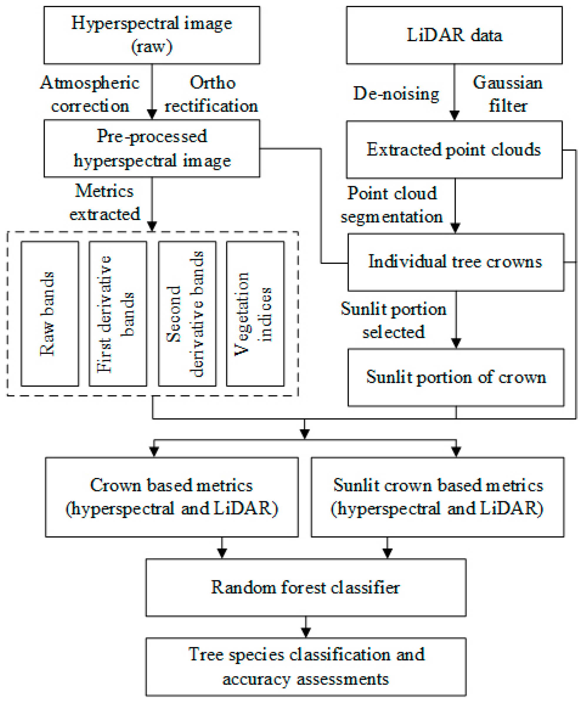
A general overview of the technique route for tree-species classification is shown in Figure 1. First, the hyperspectral raw data were preprocessed to minimize the impacts of atmospheric interference and terrain distortion. Second, four sets of metrics (raw bands, first derivative bands, second derivative bands and vegetation indices) were calculated and subsequently selected using principal component analysis (PCA). Third, each individual tree crown was extracted using point cloud segmentation algorithm (PCS) by the LiDAR data after de-noising and filtering, and then sunlit portions in each crown were selected from hyperspectral data. Finally, the LiDAR metrics computed from discrete LiDAR data within crowns and the hyperspectral metrics in individual tree crown and in sunlit portions were utilized to Random Forest classifier to discriminate five tree-species at two levels of classification.
2.1. Study Site
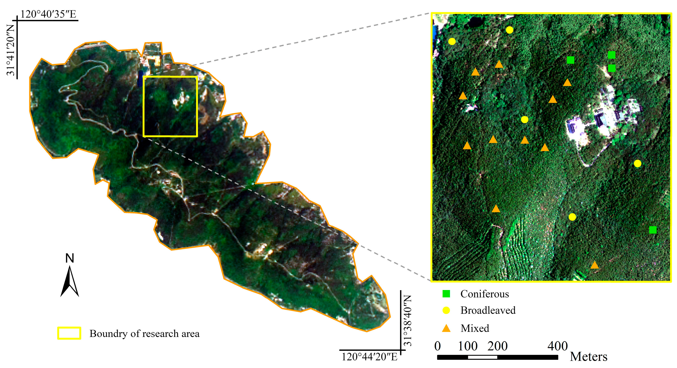
This study was conducted at Yushan Forest, a state-operated forest and national forest park, in the town of Changshu in Jiangsu Province, southeast China (120°42′9.4″E, 31°40′4.1″N) (Figure 2). It covers approximately 1103 ha, with an elevation ranging between 20 and 261 m above sea level. It is situated in the north subtropical monsoon climatic region with an annual precipitation of 1062.5 mm. The Yushan forest belongs to the north subtropical secondary forest, and it can be classified to coniferous dominated, broadleaved dominated and mixed forests [71]. The main coniferous tree-species are Chinese fir (Cunninghamia lanceolata (Lamb.) Hook.) and Masson pine (Pinus massoniana Lamb.). The major broadleaved tree-species include Sweet gum (Liquidambar formosana Hance) and Sawtooth oak (Quercus acutissima Carruth.), mixed with Chinese chestnut (Castanea mollissima BL.).
2.2. Field Data
In this study, inventory data of field plots were obtained from the forest survey (under a leaf-on condition). A total of 20 square field plots (30 × 30 m2) were established within the study site in August 2013, guided by data from an existing pre-stratified stand inventory data (2012). These plots were designed to cover a range of species composition, age classes, and site indices, and can be divided into three types based on species composition: (i) coniferous dominated forest (n = 4); (ii) broadleaved dominated forest (n = 5); and (iii) mixed species forest (n = 11). The position of the center of field plots were assessed by Trimble GeoXH6000 GPS units, corrected with high precision real-time differential signals received from the Jiangsu Continuously Operating Reference Stations (JSCORS), resulting in a sub-meter accuracy [71].
Individual tree within each plot with a diameter at breast height (DBH) larger than 5 cm was measured. The measurements included position, species, tree top height, height to crown base, and crown width in both cardinal directions. DBH was measured using a diameter tape for all trees. The calculation of position was based on the direction and distance of trees relative to the plot center. Tree top height was measured using a Vertex IV hypsometer. Crown widths were obtained as the average of two values measured along two perpendicular directions from the location of tree top. Moreover, the crown class, i.e., dominant, co-dominant, intermediate and overtopped, were also recorded. Since the intermediate and overtopped trees have little chance of being detected from above, they were excluded from the data analysis and classification. The statistics of the forest characteristics of three forest types are summarized in Table 1.
2.3. Remote Sensing Data
The hyperspectral and LiDAR data were acquired simultaneously by the LiCHy (Hyperspectral, LiDAR and CCD) Airborne Observation System [72] which was operated at 900 m above ground level with a flight path covering the entire Yushan Forest. Hyperspectral data were obtained using AISA Eagle sensor with 3.3 nm spectral resolution. The data employed were already georeferenced by the data provider. LiDAR data were acquired using a Riegl LMS-Q680i scanner with 360 kHz pulse repetition frequency and a scanning angle of ±30° from nadir. The average ground point distances of the dataset were 0.49 m (within a scanline) and 0.48 m (between scanlines) in a single scan, and the pulse density was three times higher in the overlapping regions. The specifications of hyperspectral and LiDAR data are summarized in Table 2.
2.4. Data Pre-Processing
The hyperspectral images were atmospherically corrected using the Empirical line model with the field reflectance spectra (dark and bright targets where each target recorded ten curves) obtained by ASD FieldSpec spectrometer (Analytical Spectral Devices, Boulder, CO, USA). Then, the background noise of LiDAR data was suppressed by de-noising process and smoothed by a Gaussian filter. A 0.5 m digital terrain model (DTM) and digital surface model (DSM) were created by calculating the average elevation from the ground points and highest points within each cell, respectively, and the cells that contained no points were interpolated by linear interpolation of neighboring cells. The DTM of the study area was subtracted from the elevation value of each point to compute the normalized point cloud. Finally, the geometric corrections of the hyperspectral images were implemented with a nearest-neighbor interpolation using the DSM data to minimize terrain distortions and register hyperspectral data to LiDAR data. The number of ground control points (GCP) was more than 30 in the hyperspectral image of each plots (30 × 30 m2). The overall accuracy of geometric correction was higher than 0.25 m.
2.5. Hyperspectral Metrics Calculation
The spectral reflectance is important to classify tree-species because it can be applied to record the biophysical and biochemical attributes of vegetation such as leaf area index (LAI), biomass, and presence of pigments (e.g., chlorophyll and carotenoid) [73,74,75]. All bands (64 bands) including the area of visible, red edge and near infrared were chosen in this study.
Derivative analysis is often used to enhance the target features and meanwhile weaken noises like illumination and soil background [76]. The first and second order derivatives are used most commonly. In this study, derivatives for metrics were extracted using reflectance data, and the first and second derivative bands (128 bands) were calculated.
Hyperspectral vegetation indices have been developed based on specific absorption features that quantify biophysical and biochemical indicators best. Various narrowband vegetation indices calculated from hyperspectral image helped detect and map tree-species [19,20]. Here, a set of 20 narrowband vegetation indices was calculated and summarized in Table 3. The definitions and references are presented below.
2.6. Individual Tree Detection
The point cloud segmentation (PCS) algorithm of Li et al. [52] was applied to detect individual trees. It was a top-to-bottom region growing approach to segment trees individually and sequentially from point cloud. The algorithm started from a tree top and “grow” an individual tree by including nearby points based on the relative spacing. Points with a spacing smaller than a specified threshold were classified as the target tree, and the threshold was approximately equal to the crown radius. Additionally, the shape index (SI) was added to improve the accuracy of segmentation by avoiding the elongated branch. The PCS algorithm was implemented using LiForest (GreenValley International, Berkeley, CA, USA) software, and the space threshold was equal to the mean crown radius of each corresponding forest type (coniferous = 1.45 m, broadleaved = 2.40 m and mixed = 1.91 m). The results of segmentation were point cloud which contained the attribute of tree ID, and points from the same tree had same ID. For each detected tree, the tree position, tree height and crown area were estimated and compared to the corresponding tree in the field. It was considered correct when a detected tree was located within the crown of the field inventory tree. The point cloud of detected tree was rasterized to image to match with hyperspectral image, and the value of each pixel was assigned as point ID appeared most frequently. The pixels had the same value in rasterized image were considered as a part of the same tree, and the range of crown was the boundary of pixels with the same value.
To evaluate the accuracy of tree detection, three measures including recall (r, represents the tree detection rate), precision (p, represents the precision of detected trees) and F1-score (F1, presents the overall accuracy taking both omission and commission in consideration) were introduced using the following equations [92,93].
where Nt is the number of the detected trees which exist in field position, No is the number of the trees which were omitted by algorithm, and Nc is the number of the detected trees which do not exist in field.
2.7. LiDAR Metrics Calculation
Discrete LiDAR metrics are descriptive structure statistics, and they are calculated from the height normalized LiDAR point cloud. In the study, 12 metrics for each tree were calculated, including: (i) selected height measures, i.e., percentile heights (h25, h50, h75 and h95), minimum height (hmin) and maximum height (hmax); (ii) selected canopy’s return density measures, i.e., canopy return densities (d2, d4, d6 and d8); (iii) variation of tree height, i.e., coefficient of variation of heights (hcv); and (iv) canopy cover, i.e., canopy cover above 2 m (CC). A summary of the LiDAR metrics and descriptions is given in Table 4.
Previous studies have found that first returns have more stable capabilities for forest biophysical attribute estimation than all returns [94]. Therefore, LiDAR metrics were computed by first returns. Metrics of percentile height and canopy return density were generated from first returns which were higher than 2 m above ground to exclude returns from low-lying vegetation.
2.8. Sunlit Portion in Individual Tree Crown
Previous studies have demonstrated that the spectral signal from sunlit crown was dominated by first order scattering and the impacts of soil and shadows were minimal, therefore it was appropriate for foliage or canopy modeling [95]. The sunlit crown was defined as all the pixels within an individual tree crown that had reflectance values in near infrared band greater than the mean value of crown in that band [96]. In this study, the pixels in each crown with reflectance values in 800 nm higher than the mean value were selected as sunlit crown.
2.9. Hyperspectral Metrics and the Selection
The individual tree crown and sunlit crown metrics were extracted from hyperspectral metrics using spatial statistical analysis. Metrics at the two levels both included raw reflectance bands (n = 64), derivative bands (n = 128) and vegetation indices (n = 20).
In general, hyperspectral imagery was considered to be suited for tree-species classification due to its high spectral resolution and a large amount of hyperspectral metrics. However, the high dimension of spectral data would cause Hughes phenomenon and always perform ineffectively in classification [97,98]. As result, it was necessary to optimize the hyperspectral metrics and reduce dimension of spectral data. The Principal Component Analysis (PCA) which aimed to calculate a subspace of orthogonal projections in accordance with the maximized variance of the whole metrics, therefore was widely applied in hyperspectral metrics optimization [99,100]. In this study, the PCA algorithm was used to reduce the dimension of the hyperspectral metrics. The best 20 metrics, which had high correlation with the first three principle components, were correspondingly selected from reflectance bands, derivative bands and vegetation indices at both the whole crown and sunlit crown level.
2.10. Random Forest and Classification
The Random Forest classifier is a non-parametric ensemble of decision trees which have been trained using bootstrap samples of training data. A number of trees are constructed based on random feature subset and it is faster to grow a large number of decision trees without pruning. In random forest, only the best among a subset of candidate features are selected randomly to determine the split at each node. Approximately one-third of samples that are not used in the bootstrapped training data are called the out-of-bag (OOB) samples, which offer unbiased estimates of the training error and could be used to evaluate the relative importance of features.
In total, 587 samples including Chinese chestnut (C.C: n = 117), Sweet gum (S.G: n = 100), Sawtooth oak (S.O: n = 114), Masson pine (M.P: n = 130) and Chinese fir (C.F: n = 126) were classified at two levels (five tree-species and two forest-types). Random forest classifiers were trained using training dataset, while the classification accuracies were assessed by the validation dataset. The training and validation datasets were allocated randomly, and the proportion of training dataset and validation dataset were 60% and 40%, respectively. The number of decision trees was set to 1000 to ensure that each sample was classified more than once. The classification accuracies were assessed by overall accuracy (OA), the producer’s and user’s accuracy.
In this study, the LiDAR metrics (12 metrics) and the hyperspectral metrics (80 metrics selected by the indices of PCA) were selected again using the correlation analysis (the metrics that strongly correlated with other metrics were excluded) before classification, and the number of retained LiDAR metrics and hyperspectral metrics (whole crown and sunlit crown metrics) were eight and thirty, respectively. The classification of five tree-species and two forest-types were both divided into four parts: (i) using LiDAR metrics (n = 8) and sunlit hyperspectral metrics (n = 30) to classify tree-species (SA); (ii) using LiDAR metrics (n = 8) and crown hyperspectral metrics (n = 30) to classify tree-species (CA); (iii) using sunlit hyperspectral metrics (n = 30) to classify tree-species (SH); and (iv) using crown hyperspectral metrics (n = 30) to classify tree-species (CH). In order to select the most important metrics, metrics were eliminated from random forest classifier one by one. The order in which metrics ruled out were controlled by the ranking for importance (the mean decrease in Gini index) of each metric in each loop, and the last metric was eliminated.
3. Results
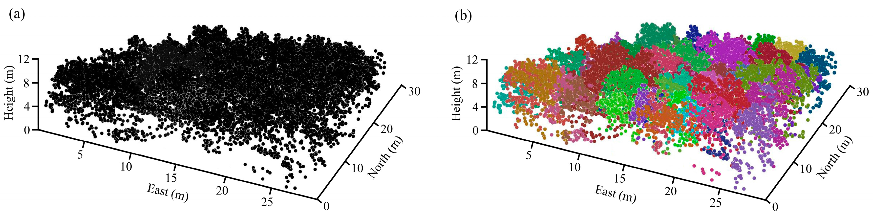
Figure 3 shows the result of individual tree detection using PCS algorithm in one plot (30 × 30 m2). Furthermore, visual inspection indicated that the algorithm succeed in segmenting subtropical forest trees. In total, 587 (80.1%) of dominate and co-dominate trees were correctly detected in all of the 20 plots. The error of omission (the number of trees which was not detected by PCS algorithm) was 146 (19.9%), and the error of commission (the number of detected trees which did not exist in the field) was 97 (14.2%). The F1-score of coniferous dominated plots was highest (88.2%), followed by the broadleaved dominated plots (85.7%), and the mixed plots was lowest (80.3%) (Table 5). It was likely due to the crown of coniferous trees which tended to be compact and relatively isolate from each other. However, the broadleaved trees were rounded and more likely to overlay, and the structure of mixed plots was more complicated than coniferous dominated and broadleaved dominated plots. The accuracy of estimated tree height and diameter were also assessed using inventory data. The accuracy of estimated crown diameter (RMSE = 0.36 m, rRMSE = 9.5% observed mean crown diameter) was less than the tree height (RMSE = 0.48 m, rRMSE = 4.6% observed mean height).
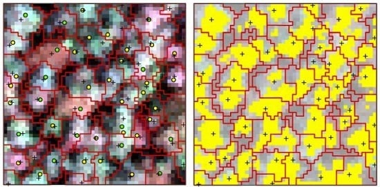
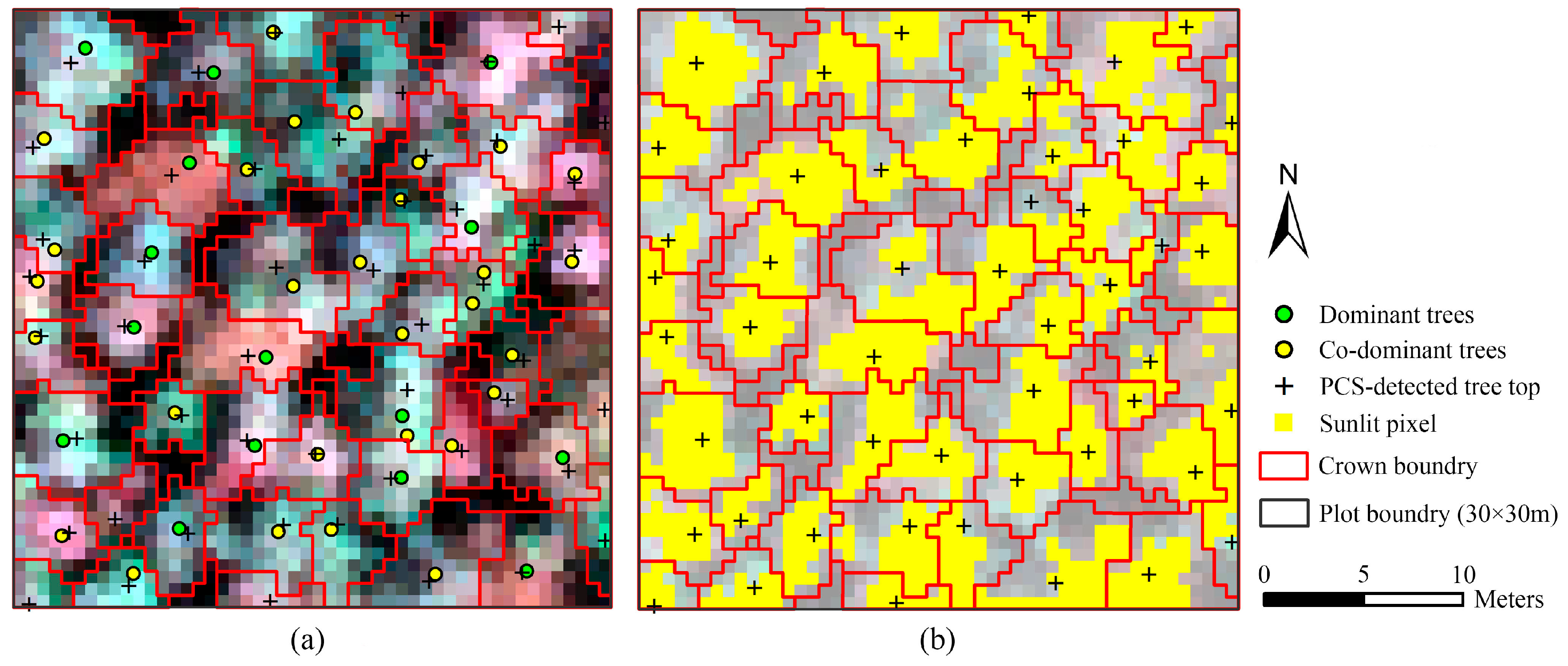
The point clouds of each tree extracted by PCS algorithm were rasterized to the image, which was matched with hyperspectral data; therefore, the boundary of each individual tree was consistent with hyperspectral image. One sample plot of hyperspectral imagery with detected tree tops, crown boundaries and the tops of linked trees in field is shown in Figure 4a. The portions in each crown with reflectance values in the band of 800 nm higher than the mean value were selected as sunlit crown. The detected trees and sunlit portion in each crown can be seen in Figure 4b.
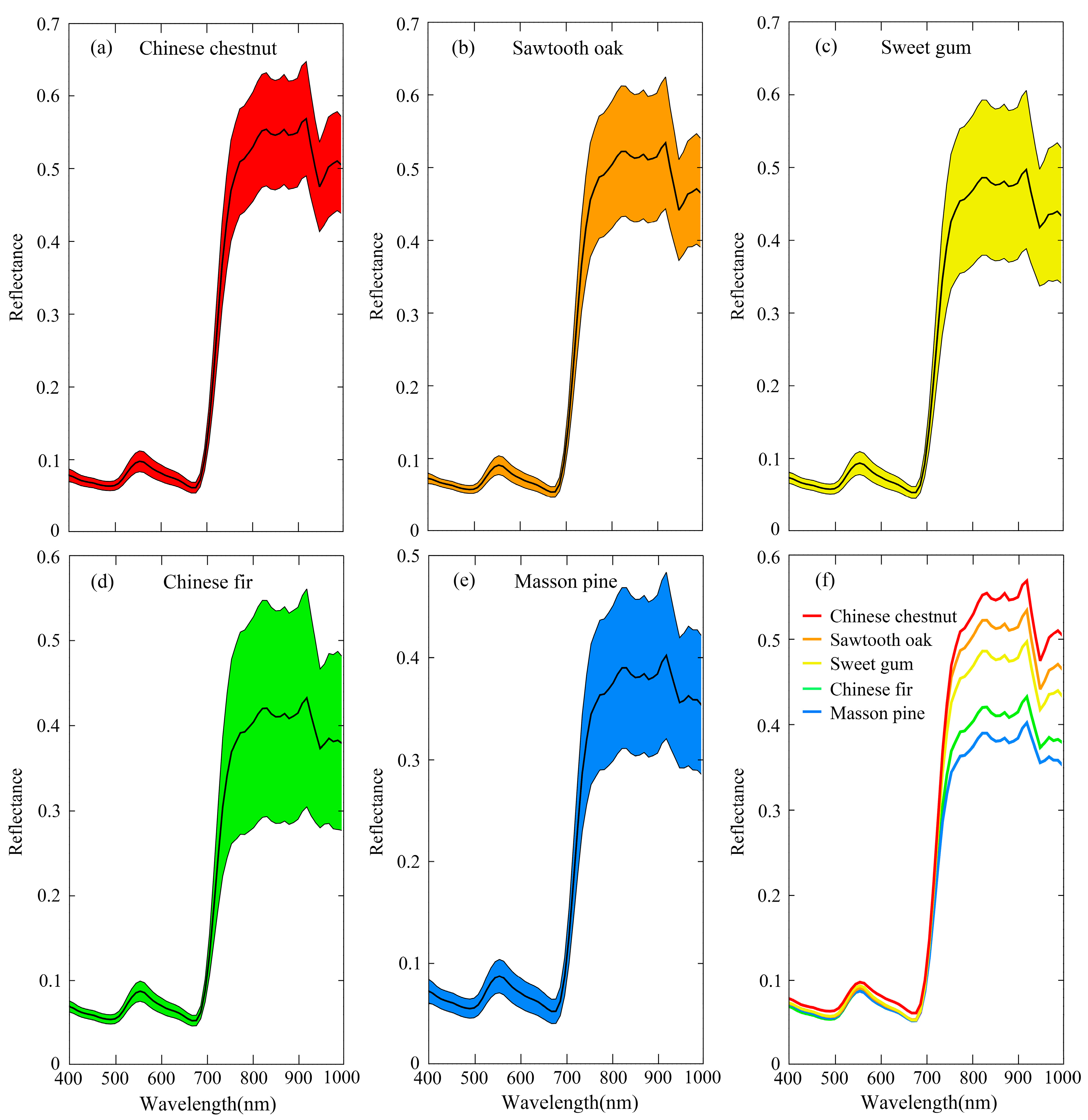
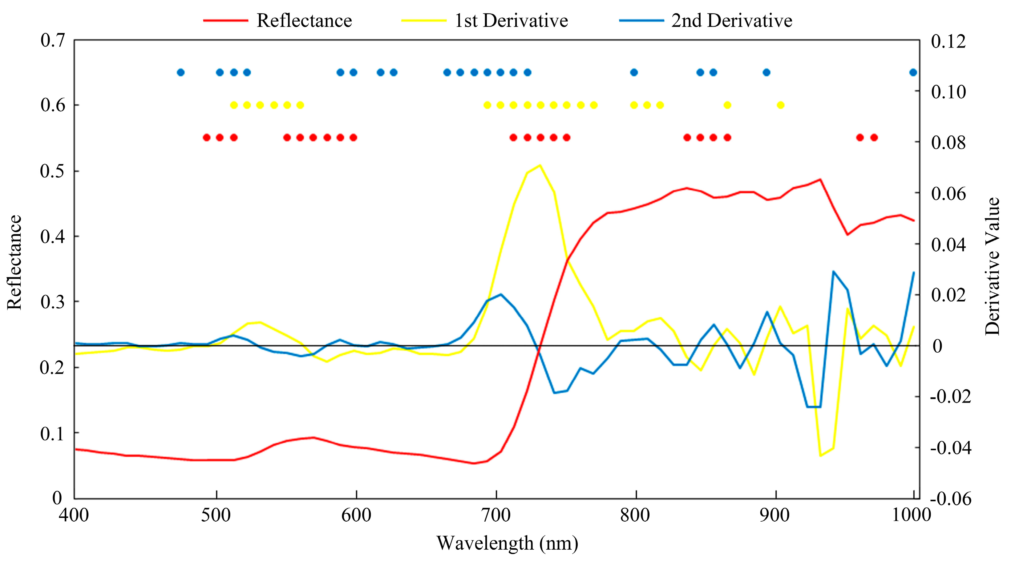
The reflectance of five tree-species extracted from sunlit crown indicated that the species exhibited various spectral responses, especially in the areas of near infrared. It was noted by the difference sizes of envelopes (Figure 5a–e) and the mean spectral reflectance in Figure 5f. The hyperspectral metrics were also calculated based on this premise. With the PCA algorithm, 20 best metrics were correspondingly selected from reflectance bands, derivative bands and vegetation indices at both whole crown and sunlit crown level. The result of best metrics selected from sunlit crown metrics is shown in Figure 6. The metrics are mainly located in the regions of visible, red edge and near infrared.
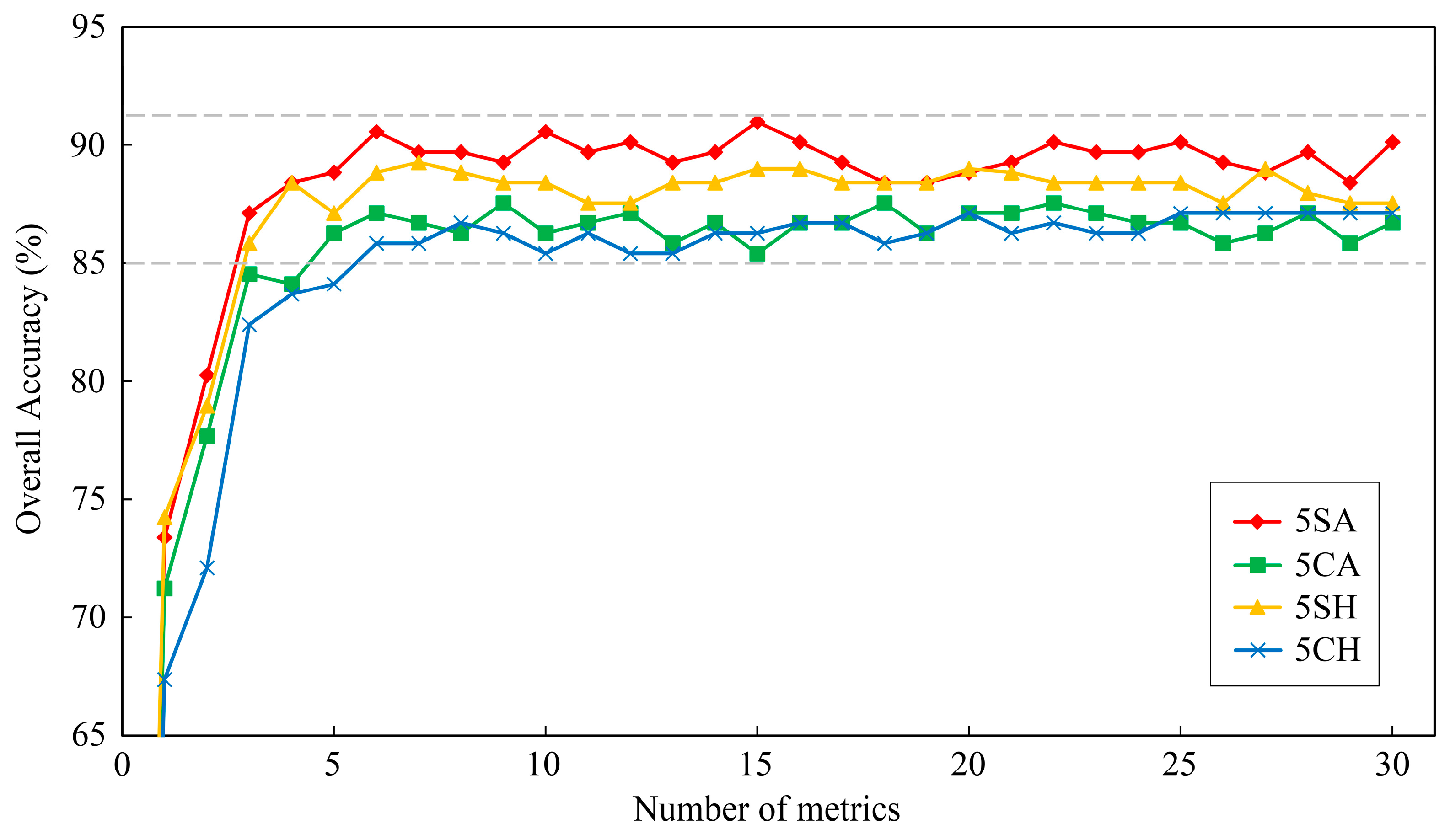
Figure 7 presents the overall accuracies of five tree-species classifications using random forest classifier with respect to the reduction of metrics numbers (0–30). When the number of metrics was less than six, the overall accuracies of classifications decreased by the reduction of the number of metrics in most cases. Then, the overall accuracies were tend to be stable at the certain numerical range when metrics number was larger than six. Therefore, only few selected metrics could be used to classify tree-species effectively, and six was the optimal number of metrics for five tree-species classifications in this study. The top-six important metrics were selected as the most important metrics for five tree-species classifications (Table 6). Classification using LiDAR and sunlit hyperspectral metrics (5SA) performed best, followed by classification using sunlit hyperspectral metrics (5SH) and classification using LiDAR and crown hyperspectral metrics (5CA), and the classification using crown hyperspectral metrics (5CH) performed worst. The classifications using LiDAR and hyperspectral metrics had better performance than classifications using only hyperspectral metrics; therefore, the fusion of hyperspectral and LiDAR data could improve the accuracy of tree-species classification in subtropical forests. In addition, the classifications using sunlit crown metrics also outperformed the classifications using whole crown metrics, which indicated that the metrics extracted from sunlit crown had lower within-species variance and could be used to enhance the species separability.
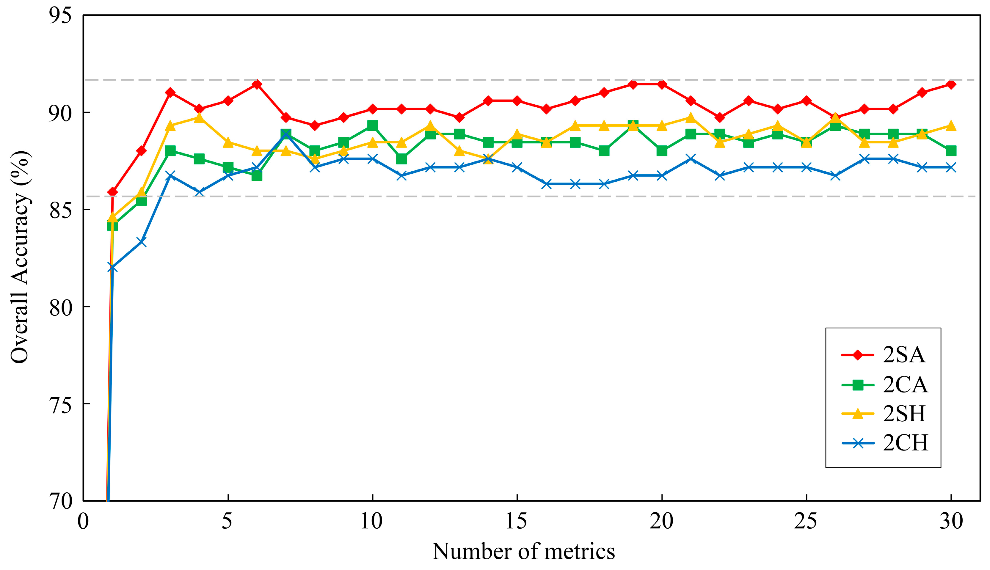
Similarly, Figure 8 displays the overall accuracies of two forest-types classifications with respect to the reduction of metrics number (0–30). When the number of metrics was less than three, the overall accuracies of classifications decreased by the reduction of the number of metrics in all cases. Then, the overall accuracies tended to be stable at certain numerical range when metrics number was larger than three. Therefore, only few selected metrics could also be used to classify forest types effectively, and three was the optimal number of metrics for two forest-types classification in this study. The top-three important metrics were selected as the most important metrics for two forest-types classification (Table 6). For two forest-types classification, classification using LiDAR and sunlit hyperspectral metrics (2SA) performed best, followed by classification using sunlit hyperspectral metrics (2SH) and classification using LiDAR and crown hyperspectral metrics (2CA), and the classification using crown hyperspectral metrics (2CH) performed worst. The classifications using LiDAR and hyperspectral metrics had better performance than classifications using only hyperspectral metrics, which demonstrated that the fusion of hyperspectral and LiDAR data could also improve the accuracy of two forest-types classification in subtropical forests. Meanwhile, the classifications using sunlit crown metrics outperformed the classifications using whole crown metrics, and it indicated that the metrics extracted from sunlit crown had lower within-type variance and could be used to enhance the separability of forest types as well.
The confusion matrix and accuracies of classifications using the most important metrics at two classification levels, i.e., all five tree-species and two forest-types are shown in Table 7 and Table 8, respectively. Classifications of two forest-types using three most important metrics (overall accuracy = 86.7–91.0%) have slightly higher accuracies than the classifications of five tree-species using six most important metrics (overall accuracy = 85.8–90.6%). In both classifications of five tree-species and two forest-types, classification using LiDAR and sunlit hyperspectral metrics had highest accuracy (overall accuracy = 90.6% and 91.0%), followed by classification using sunlit hyperspectral metrics (overall accuracy = 88.8% and 89.3%) and classification using LiDAR and crown hyperspectral metrics (overall accuracy = 87.1% and 88.0%), sequentially, and the classification using crown hyperspectral metrics had lowest accuracy (overall accuracy = 85.8% and 86.7%). The classifications using LiDAR and hyperspectral metrics (overall accuracy = 87.1–91.0%) performed better than the classifications using only hyperspectral metrics (overall accuracy = 85.8–89.3%), and the classifications using sunlit crown metrics (overall accuracy = 88.8–91.0%) outperformed using whole crown metrics (overall accuracy = 85.8–88.0%).
4. Discussion
The tree-species classification would have better performance because the fusion of hyperspectral and LiDAR data could achieve the combination of spectral and structure information [62,63,101]. In this study, although the classifications using hyperspectral metrics showed a relative good performance (overall accuracies were stable over 85%), the classifications using LiDAR and hyperspectral metrics performed better and had higher accuracies. Moreover, the improvements of overall accuracies were from 0.4% to 5.6% except few cases caused by the effect of Hughes phenomenon (Figure 7 and Figure 8). Furthermore, compared with the classifications using only hyperspectral metrics, the mean omission and commission of classifications using LiDAR and hyperspectral metrics decreased by 1.5% and 1.6%, respectively (Table 7 and Table 8). Cao et al. [16] classified tree-species using only full-waveform LiDAR data with random forest classifier in the same study area of subtropical forests. Compared with our results, lower overall accuracies were obtained in six tree-species (68.6%) and two forest-types (86.2%) classification. Alonzo et al. [63] reported a 4.2% increase of classification overall accuracy for the addition of LiDAR data to hyperspectral metrics in urban forests located on Santa Barbara, California. Jones et al. [23] classified 11 tree-species using the fused hyperspectral and LiDAR data at pixel-level in temperate forests of coastal southwestern Canada and found that the producer’s accuracy increased 5.1–11.6% compared with using single dataset, which was slightly higher than reported in this study. The reason for the slight lower improvement of accuracy in our study may be due to the complexity of multilayered subtropical forest which decline the capability of LiDAR metrics to discriminate tree-species.
Traditionally, the individual tree crown (ITC) was manually delineated on RGB false color image, or automatically delineated based on image segmentation algorithm on optical image and LiDAR-derived canopy height model (CHM). The result of crown delineation using optical image was influenced by the image quality which depended on many factors (e.g., sensor status, illumination and view geometry), and the segmentation algorithm using LiDAR-derived CHM was not ideal as the CHM which had inherent errors during the interpolating process from point cloud to gridded model. The PCS algorithm is a method to segment individual tree from point cloud directly. It could provide three dimensional structure information of each tree and avoid the limitation of using CHM. In this study, the PCS algorithm was a top-to-bottom region growing approach that segmented trees individually and sequentially from point cloud. In total, 587 (80.1%) of dominate and co-dominate trees were correctly detected and the overall accuracy was 82.9%. Cao et al. [16] applied local maximum filtering algorithm to detect individual tree in the same research area, and the 78.5% of dominate and co-dominate trees were correctly detected. The slightly lower detection accuracy compared with this study may be caused by the errors of CHM and the smooth median filtering. The accuracy of estimated crown diameter (rRMSE = 9.5%) by PCS algorithm was lower than tree height (rRMSE = 4.6%), which may be owing to the overlapping of adjacent canopy in subtropical forest.
Based on the selected result of hyperspectral metrics extracted from sunlit crown using PCA algorithm (Figure 6), three spectral regions were identified. Two regions in the visible band (500–600 nm and 680–750 nm) included blue edge, green peak, part of yellow edge, red valley and red edge. Previous studies had used these bands to separate tree-species at various scales [20,102,103]. They were related to nitrogen, pigment content, vegetation vigor, light use efficiency, plant stress and biophysical quantities, and all these properties were supposed to differ among species [104,105,106]. The other region was in the near infrared band (800–900 nm) which had high reflectance due to multiple-scattering within leaf structure such as spongy mesophyll. The region was related to cell structure, biophysical quantity and yield (e.g., biomass and LAI) [107,108]. Clark et al. [15] found that the species differences were mainly focused in NIR region at canopy scale. It was also confirmed in this study that the difference of five tree-species was maximum in NIR bands (Figure 5f).
In hyperspectral image, the crown spectral values may exhibit bimodal tendencies related to the sunlit and shadow parts [96], and the multiple-scattering among tree crown may lead to noisy spectral values. The sunlit crown values were dominated by first-order scattering from canopy and the influences of soil background, trunk and branch were minimum. Therefore, using metrics extracted from sunlit crown may improve the classification accuracy. This hypothesis was confirmed by our results that the classifications using sunlit crown metrics (overall accuracies stable at 87.1–91.5%) had better performance than using whole crown metrics (overall accuracies stable at 85.4–89.3%), and the mean improvement of overall accuracy was 2.3% (Figure 7 and Figure 8). The classification of 17 tree-species in tropical forests undertaken by Feret et al. [13] showed similar results. Meanwhile, compared with the classifications using whole crown metrics, the omission and commission of classifications using sunlit metrics were declined 0–7.5% and 0–8.6%, respectively (Table 7 and Table 8).
With the one by one elimination of the input selected metrics after decorrelation, the overall accuracies were stable at certain numerical range (standard deviation = 0.53–0.64%) at the beginning, and then started decrease since the remaining metrics could not provide sufficient information for species discrimination. The number of input metrics of last point before the decline of overall accuracies was seen as the optimal number of metrics for classification. In this study, six and three were the optimal number of metrics for five tree-species and two forest-types classification, respectively. The top-ranked six or three metrics were selected as the most important metrics. Compared with highest overall accuracies of each classification, the overall accuracies of five tree-species and two forest-types classification using the most important metrics descended only 0.4–1.3% and 0.4–2.1%, respectively. Therefore, the classifications using the most important metrics improved the overall accuracies significantly and these metrics could be used to classify tree-species efficiently, which is consistent with the previous studies [16,99].
The point clouds metrics have significant relationship with three dimensional structure proprieties of canopy [57,109,110]. During the classifications, the LiDAR metrics hcv, h95 and d2 were selected as the most important metrics (Table 6). hcv indicated the height variation of all first returns, and it could reflect the canopy structure of different species. At the study site, coniferous trees usually have dense and homogenous tower-shaped crown which lead to a relative low height variance of first return within crown. Meanwhile, the broadleaved trees have loose and heterogeneous ovoid crown which lead to a high height variance of first return within crown. hcv is sensitive to this difference, which makes it possible to be a good metric for species discrimination. h95 is also a good indicator of classifying tree-species since it is upper percentile height which can reflect the height of trees in some extent. Furthermore, the forest in study area is under a mature or near mature condition, therefore, the tree height is approaching the maximum value, resulting the differences of height among different species. d2 is the percentage of first return above the 20 quantiles to total number of first returns, and the crown with dense foliage and branch could reduce the number of points in lower height, thereby d2 could be used to describe the dense of crown. The species with different crown density will lead to the various d2, and thus it could be effectively applied to classify tree-species.
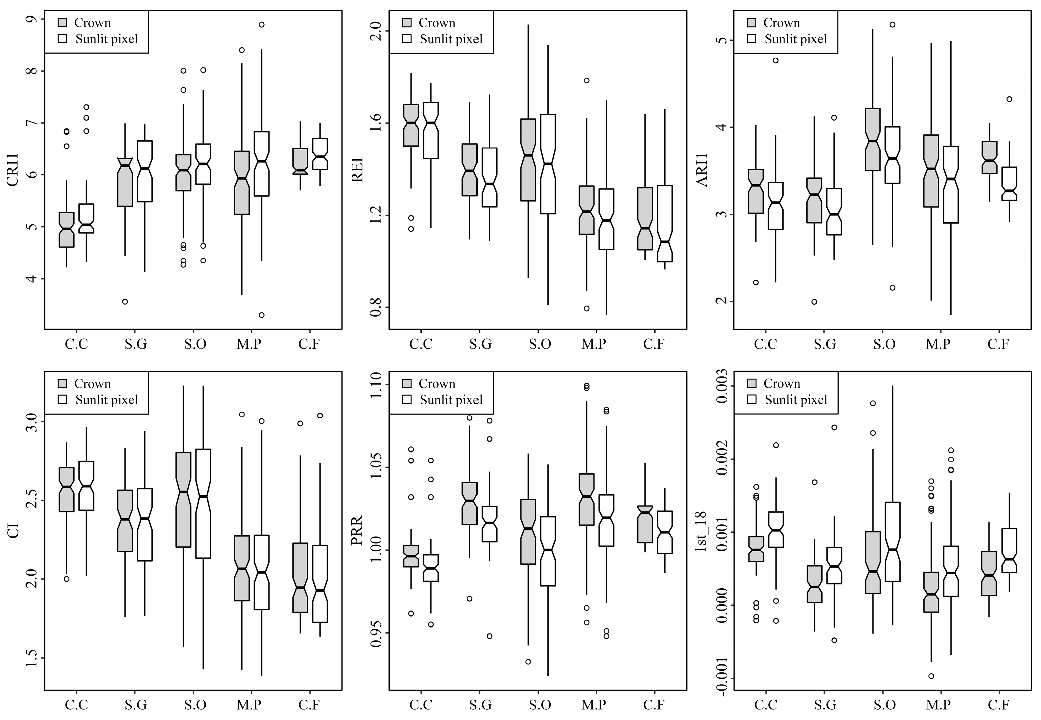
Previous studies have verified the significant effects of hyperspectral metrics for tree-species classification [13,63], and this study also showed the obvious advantages of hyperspectral metrics. The overall accuracies of classifications using only hyperspectral metrics were greater than 85% and the overall accuracies were higher after adding LiDAR metrics. Six frequently used hyperspectral metrics (i.e., CRI1, REI, ARI1, CI, PRR and 1st_18) were selected from the most important metrics. For each metric, the differences of five tree-species are significant (Figure 9). CRI1, ARI1 and CI are metrics representing reflectance of carotenoid, anthocyanin and chlorophyll, respectively, and are correlated with the content of pigments directly. Therefore, the content of pigments in five tree-species will lead these three metrics to vary with different tree-species. Gitelson et al. [84] found that REI had a strong relationship with canopy content of chlorophyll (R2 = 0.94, RMSE = 0.15 g/m2), and can be used to estimate the content of chlorophyll accurately. Therefore, it was applied to classify tree-species effectively in this study, and the distribution of box plot was similar to CI. PRR is a metrics used to measure the efficiency of light use which may be influenced by content of pigments and the crown surface structure. As a result, tree-species (e.g., Masson pine) with high content of pigments and dense crown have high light use efficiency. It has been proved that classification using first-order derivative metrics outperformed using reflectance metrics [111]. 1st_18 is the value of first-order derivative in 553 nm correlated with chlorophyll and biomass which can be used to assess vegetation fertility level and biophysical quantity, thus it is a good indicator to classify five tree-species in subtropical forest.
To compare the six metrics selected from most important metrics, CRI1, ARI1, PRR and 1st_18 were all calculated using green bands, and REI and CI were calculated using red edge bands. Green band and red edge region were both verified as informative areas of spectrum in vegetation studies [112], which is similar with the results of band selection using PCA algorithm (Figure 6). CRI1, ARI1, PRR and 1st_18 all had different values in sunlit crown and whole crown, yet the ranges of REI and CI in sunlit crown and whole crown were similar (Figure 9). Therefore, CRI1, ARI1, PRR and 1st_18 might be more sensitive to illumination than REI and CI. It could be explained that the green bands had shorter wavelength and the value was more likely influenced by scattering in crown than red edge bands [113].
5. Conclusions
In this study, we used simultaneously acquired hyperspectral and LiDAR data from LiCHy (Hyperspectral, LiDAR and CCD) airborne system to classify five tree-species (in two classification depths) in subtropical forests of southeast China. The results showed that the tree delineation approach (point cloud segmentation algorithm) was suitable for detecting individual tree in this study (overall accuracy = 82.9%). The classification approach provided a relative high accuracy for classifying tree-species in the study site (overall accuracy > 85.4% for five tree species and overall accuracy > 86.3% for two forest-types). The classification using both hyperspectral and LiDAR metrics resulted in higher accuracies than only hyperspectral metrics (the improvement of overall accuracies = 0.4–5.6%). In addition, the classifications using sunlit crown metrics (overall accuracies = 87.1–91.5%) had improved the overall accuracies of 2.3%, compared with the classification using whole crown metrics (overall accuracies = 85.4–89.3%). The results also suggested that fewer of the most important metrics can be used to classify tree-species effectively (overall accuracies = 85.8–91.0%).
Although this study shows significant potential for combined hyperspectral and LiDAR data to classify tree-species in subtropical forests, more advanced spectral and structure metrics need to be explored and the high spatial resolution data, which were acquired simultaneously by the LiCHy Airborne Observation System, can be fused with the hyperspectral and LiDAR data in the future work to enhance the capability of tree-species classification in subtropical forests.
Acknowledgments
The project was funded by the Natural Science Foundation of China (No. 31400492) and the Natural Science Foundation of Jiangsu Province (No. BK20151515). This research was also supported by the Priority Academic Program Development of Jiangsu Higher Education Institutions (PAPD). Special thanks to Jinsong Dai, Kun Liu, and Ting Xu for fieldwork. The authors gratefully acknowledge the foresters in Yushan forest for their assistance with data collection and sharing their rich knowledge and working experience of the local forest ecosystems.
Author Contributions
Xin Shen analyzed the data and wrote the paper. Lin Cao helped in project and study design, paper writing, and analysis.
Conflicts of Interest
The authors declare no conflict of interest.
References
- Food and Agriculture Organization (FAO). Global Forest Resources Assessment; Food and Agriculture Organization: Rome, Italy, 2010; Volume 163. [Google Scholar]
- Pan, Y.; Birdsey, R.A.; Phillips, O.L.; Jackson, R.B. The structure, distribution, and biomass of the worlds forests. Annu. Rev. Ecol. Evol. Syst. 2013, 44, 593–622. [Google Scholar] [CrossRef]
- McKinley, D.C.; Ryan, M.G.; Birdsey, R.A.; Giardina, C.P.; Harmon, M.E.; Heath, L.S.; Houghton, R.A.; Jackson, R.B.; Morrison, J.F.; Murray, B.C.; et al. A synthesis of current knowledge on forests and carbon storage in the United States. Ecol. Appl. 2011, 21, 1902–1924. [Google Scholar] [CrossRef] [PubMed]
- Walther, G.-R.; Post, E.; Convey, P.; Menzel, A.; Parmesan, C.; Beebee, T.J.C.; Fromentin, J.-M.; Hoegh-Guldberg, O.; Bairlein, F. Ecological responses to recent climate change. Nature 2002, 416, 389–395. [Google Scholar] [CrossRef] [PubMed]
- Clark, J.S.; McLachlan, J.S. Stability of forest biodiversity. Nature 2003, 423, 635–638. [Google Scholar] [CrossRef] [PubMed]
- Lin, D.; Lai, J.; Muller-Landau, H.C.; Mi, X.; Ma, K. Topographic variation in aboveground biomass in a subtropical evergreen broad-leaved forest in China. PLoS ONE 2012, 7. [Google Scholar] [CrossRef] [PubMed]
- Wang, X.-H.; Kent, M.; Fang, X.-F. Evergreen broad-leaved forest in Eastern China: Its ecology and conservation and the importance of resprouting in forest restoration. For. Ecol. Manag. 2007, 245, 76–87. [Google Scholar] [CrossRef]
- Plourde, L.C.; Ollinger, S.V.; Smith, M.L.; Martin, M.E. Estimating species abundance in a northern temperate forest using spectral mixture analysis. Photogramm. Eng. Remote Sens. 2007, 73, 829–840. [Google Scholar] [CrossRef]
- Cho, M.A.; Mathieu, R.; Asner, G.P.; Naidoo, L.; van Aardt, J.; Ramoelo, A.; Debba, P.; Wessels, K.; Main, R.; Smit, I.P.J.; et al. Mapping tree species composition in South African savannas using an integrated airborne spectral and LiDAR system. Remote Sens. Environ. 2012, 125, 214–226. [Google Scholar] [CrossRef]
- Dale, V.H.; Joyce, L.A.; Mcnulty, S.; Neilson, R.P.; Ayres, M.P.; Flannigan, M.D.; Hanson, P.J.; Irland, L.C.; Lugo, A.E.; Peterson, C.J.; et al. Climate change and forest disturbances. Bioscience 2001, 51, 723. [Google Scholar] [CrossRef]
- Thomas, S.C.; Malczewski, G. Wood carbon content of tree species in Eastern China: Interspecific variability and the importance of the volatile fraction. J. Environ. Manag. 2007, 85, 659–662. [Google Scholar] [CrossRef] [PubMed]
- Foody, G.M. Remote sensing of tropical forest environments: Towards the monitoring of environmental resources for sustainable development. Int. J. Remote Sens. 2003, 24, 4035–4046. [Google Scholar] [CrossRef]
- Feret, J.-B.; Asner, P.G. Tree species discrimination in tropical forests using airborne imaging spectroscopy. IEEE Trans. Geosci. Remote Sens. 2013, 51, 73–84. [Google Scholar] [CrossRef]
- Li, J.; Hu, B.; Noland, T.L. Classification of tree species based on structural features derived from high density LiDAR data. Agric. For. Meteorol. 2013, 171–172, 104–114. [Google Scholar] [CrossRef]
- Clark, M.L.; Roberts, D.A.; Clark, D.B. Hyperspectral discrimination of tropical rain forest tree species at leaf to crown scales. Remote Sens. Environ. 2005, 96, 375–398. [Google Scholar] [CrossRef]
- Cao, L.; Coops, N.C.; Innes, J.L.; Dai, J.; Ruan, H.; She, G. Tree species classification in subtropical forests using small-footprint full-waveform LiDAR data. Int. J. Appl. Earth Obs. Geoinf. 2016, 49, 39–51. [Google Scholar] [CrossRef]
- Souza, A.F.; Forgiarini, C.; Longhi, S.J.; Oliveira, J.M. Detecting ecological groups from traits: A classification of subtropical tree species based on ecological strategies. Braz. J. Bot. 2014, 37, 441–452. [Google Scholar] [CrossRef]
- Li, L.; Huang, Z.; Ye, W.; Cao, H.; Wei, S.; Wang, Z.; Lian, J.; Sun, I.F.; Ma, K.; He, F. Spatial distributions of tree species in a subtropical forest of China. Oikos 2009, 118, 495–502. [Google Scholar] [CrossRef]
- Dalponte, M.; Ørka, H.O.; Gobakken, T.; Gianelle, D.; Næsset, E. Tree species classification in boreal forests with hyperspectral data. IEEE Trans. Geosci. Remote Sens. 2013, 51, 2632–2645. [Google Scholar] [CrossRef]
- Clark, M.L.; Roberts, D.A. Species-level differences in hyperspectral metrics among tropical rainforest trees as determined by a tree-based classifier. Remote Sens. 2012, 4, 1820–1855. [Google Scholar] [CrossRef]
- Shaw, G.; Manolakis, D. Signal processing for hyperspectral image exploitation. IEEE Signal Process. Mag. 2002, 19, 12–16. [Google Scholar] [CrossRef]
- Odagawa, S.; Okada, K. Tree species discrimination using continuum removed airborne hyperspectral data. 2009 First Work. Hyperspectral Image Signal Process. Evol. Remote Sens. 2009, 1–4. [Google Scholar] [CrossRef]
- Jones, T.G.; Coops, N.C.; Sharma, T. Assessing the utility of airborne hyperspectral and LiDAR data for species distribution mapping in the coastal Pacific Northwest, Canada. Remote Sens. Environ. 2010, 114, 2841–2852. [Google Scholar] [CrossRef]
- Richter, R.; Reu, B.; Wirth, C.; Doktor, D.; Vohland, M. The use of airborne hyperspectral data for tree species classification in a species-rich Central European forest area. Int. J. Appl. Earth Obs. Geoinf. 2016, 52, 464–474. [Google Scholar] [CrossRef]
- Erins, G.; Lorencs, A.; Mednieks, I.; Sinica-Sinavskis, J. Tree species classification in mixed Baltic forest. In Proceedings of the Workshop on Hyperspectral Image and Signal Processing: Evolution in Remote Sensing (WHISPERS), Lisbon, Portugal, 6–9 June 2011; pp. 1–4. [Google Scholar]
- Krahwinkler, P.; Rossmann, J. Tree Species Classification Based on the Analysis of Hyperspectral Remote Sensing Data. In Proceedings of the Geoscience and Remote Sensing Symposium (IGARSS), Beijing, China, 10–15 July 2016; pp. 321–328. [Google Scholar]
- Melgani, F.; Bruzzone, L. Classification of hyperspectral remote sensing images with support vector machines. IEEE Trans. Geosci. Remote Sens. 2004, 42, 1778–1790. [Google Scholar] [CrossRef]
- Fung, T.; Ma, F.Y.; Siu, W.L. Hyperspectral data analysis for subtropical tree species recognition. In Proceedings of the 1998 Geoscience and Remote Sensing Symposium, Seattle, WA, USA, 6–10 July 1998; Volume 3, pp. 1298–1300. [Google Scholar]
- Jensen, R.R.; Hardin, P.J.; Hardin, A.J. Classification of urban tree species using hyperspectral imagery. Geocarto Int. 2012, 27, 443–458. [Google Scholar] [CrossRef]
- Youngentob, K.N.; Roberts, D.A.; Held, A.A.; Dennison, P.E.; Jia, X.; Lindenmayer, D.B. Mapping two Eucalyptus subgenera using multiple endmember spectral mixture analysis and continuum-removed imaging spectrometry data. Remote Sens. Environ. 2011, 115, 1115–1128. [Google Scholar] [CrossRef]
- Boschetti, M.; Boschetti, L.; Oliveri, S.; Casati, L.; Canova, I. Tree species mapping with Airborne hyperspectral MIVIS data: The Ticino Park study case. Int. J. Remote Sens. 2007, 28, 1251–1261. [Google Scholar] [CrossRef]
- Delegido, J.; Verrelst, J.; Meza, C.M.; Rivera, J.P.; Alonso, L.; Moreno, J. A red-edge spectral index for remote sensing estimation of green LAI over agroecosystems. Eur. J. Agron. 2013, 46, 42–52. [Google Scholar] [CrossRef]
- Yu, Q.; Gong, P.; Clinton, N.; Biging, G.; Kelly, M.; Schirokauer, D. Object-based detailed vegetation classification with airborne high spatial resolution remote sensing imagery. Photogramm. Eng. Remote Sens. 2006, 72, 799–811. [Google Scholar] [CrossRef]
- Heinzel, J.; Koch, B. Investigating multiple data sources for tree species classification in temperate forest and use for single tree delineation. Int. J. Appl. Earth Obs. Geoinf. 2012, 18, 101–110. [Google Scholar] [CrossRef]
- Tarabalka, Y.; Chanussot, J.; Benediktsson, J.A. Segmentation and classification of hyperspectral images using watershed transformation. Pattern Recognit. 2010, 43, 2367–2379. [Google Scholar] [CrossRef]
- Van Aardt, J.A.N.; Wynne, R.H. Examining pine spectral separability using hyperspectral data from an airborne sensor: An extension of field-based results. Int. J. Remote Sens. 2007, 28, 431–436. [Google Scholar] [CrossRef]
- Biging, G.S.; Dobbertin, M. Evaluation of Competition Indices in Individual Tree Growth-Models. For. Sci. 1995, 41, 360–377. [Google Scholar] [CrossRef]
- Fox, J.C.; Ades, P.K.; Bi, H. Stochastic structure and individual-tree growth models. For. Ecol. Manag. 2001, 154, 261–276. [Google Scholar] [CrossRef]
- Medlyn, B.E.; Pepper, D.A.; O’Grady, A.P.; Keith, H. Linking leaf and tree water use with an individual-tree model. Tree Physiol. 2007, 27, 1687–1699. [Google Scholar] [CrossRef] [PubMed]
- Mõttus, M.; Takala, T. A forestry GIS-based study on evaluating the potential of imaging spectroscopy in mapping forest land fertility. Int. J. Appl. Earth Obs. Geoinf. 2014, 33, 302–311. [Google Scholar] [CrossRef]
- Robila, S.A. An investigation of spectral metrics in hyperspectral image preprocessing for classification. In Proceedings of the ASPRS Annual Conference, Baltimore, MD, USA, 7–11 March 2005. [Google Scholar]
- Singh, A.K.; Kumar, H.V.; Kadambi, G.R.; Kishore, J.K.; Shuttleworth, J.; Manikandan, J. Quality metrics evaluation of hyperspectral images. In Proceedings of the International Archives of the Photogrammetry Remote Sensing and Spatial Information Sciences, ISPRS Technical Commission VIII Symposium, Hyderabad, India, 9–12 December 2014; Volume 40, pp. 1221–1226. [Google Scholar]
- Ollinger, S.V.; Smith, M.-L. Net primary production and canopy nitrogen in a temperate forest landscape: An analysis using imaging spectroscopy, modeling and field data. Ecosystems 2005, 8, 760–778. [Google Scholar] [CrossRef]
- Pu, R.; Gong, P.; Heald, R. In situ hyperspectral data analysis for nutrient estimation of giant sequoia. Geosci. Remote Sens. 1999, 395–397. [Google Scholar] [CrossRef]
- Gitelson, A.A.; Zur, Y.; Chivkunova, O.B.; Merzlyak, M.N. Assessing carotenoid content in plant leaves with reflectance spectroscopy. Photochem. Photobiol. 2002, 75, 272–281. [Google Scholar] [CrossRef]
- Gitelson, A.A.; Merzlyak, M.N.; Chivkunova, O.B. Optical properties and nondestructive estimation of anthocyanin content in plant leaves. Photochem. Photobiol. 2001, 74, 38–45. [Google Scholar] [CrossRef]
- Fagan, M.E.; DeFries, R.S.; Sesnie, S.E.; Arroyo-Mora, J.P.; Soto, C.; Singh, A.; Townsend, P.A.; Chazdon, R.L. Mapping species composition of forests and tree plantations in northeastern Costa Rica with an integration of hyperspectral and multitemporal landsat imagery. Remote Sens. 2015, 7, 5660–5696. [Google Scholar] [CrossRef]
- Drake, J.B.; Dubayah, R.O.; Knox, R.G.; Clark, D.B.; Blair, J.B. Sensitivity of large-footprint lidar to canopy structure and biomass in a neotropical rainforest. Remote Sens. Environ. 2002, 81, 378–392. [Google Scholar] [CrossRef]
- Koetz, B.; Morsdorf, F.; Sun, G.; Ranson, K.J.; Itten, K.; Allgöwer, B. Inversion of a lidar waveform model for forest biophysical parameter estimation. IEEE Geosci. Remote Sens. Lett. 2006, 3, 49–53. [Google Scholar] [CrossRef]
- Hyyppa, J.; Kelle, O.; Lehikoinen, M.; Inkinen, M. A segmentation-based method to retrieve stem volume estimates from 3-D tree height models produced by laser scanners. IEEE Trans. Geosci. Remote Sens. 2001, 39, 969–975. [Google Scholar] [CrossRef]
- Ene, L.; Næsset, E.; Gobakken, T. Single tree detection in heterogeneous boreal forests using airborne laser scanning and area-based stem number estimates. Int. J. Remote Sens. 2012, 33, 5171–5193. [Google Scholar] [CrossRef]
- Li, W.; Guo, Q.; Jakubowski, M.K.; Kelly, M. A new method for segmenting individual trees from the Lidar point cloud. Photogramm. Eng. Remote Sens. 2012, 78, 75–84. [Google Scholar] [CrossRef]
- Wang, Y.; Weinacker, H.; Koch, B. A Lidar point cloud based procedure for vertical canopy structure analysis and 3D single tree modelling in forest. Sensors 2008, 8, 3938–3951. [Google Scholar] [CrossRef] [PubMed]
- Andersen, H.-E.; Reutebuch, S.E.; McGaughey, R.J. A rigorous assessment of tree height measurements obtained using airborne lidar and conventional field methods. Can. J. Remote Sens. 2006, 32, 355–366. [Google Scholar] [CrossRef]
- Lim, K.; Treitz, P.; Wulder, M.; St-Onge, B.; Flood, M. LiDAR remote sensing of forest structure. Prog. Phys. Geogr. 2003, 27, 88–106. [Google Scholar] [CrossRef]
- Kim, S.; McGaughey, R.J.; Andersen, H.-E.; Schreuder, G. Tree species differentiation using intensity data derived from leaf-on and leaf-off airborne laser scanner data. Remote Sens. Environ. 2009, 113, 1575–1586. [Google Scholar] [CrossRef]
- Ørka, H.O.; Næsset, E.; Bollandsås, O.M. Classifying species of individual trees by intensity and structure features derived from airborne laser scanner data. Remote Sens. Environ. 2009, 113, 1163–1174. [Google Scholar] [CrossRef]
- Liu, L.; Coops, N.C.; Aven, N.W.; Pang, Y. Mapping urban tree species using integrated airborne hyperspectral and LiDAR remote sensing data. Remote Sens. Environ. 2017, 200, 170–182. [Google Scholar] [CrossRef]
- Vaughn, N.R.; Moskal, L.M.; Turnblom, E.C. Tree species detection accuracies using discrete point lidar and airborne waveform lidar. Remote Sens. 2012, 4, 377–403. [Google Scholar] [CrossRef]
- Holmgren, J.; Persson, Å. Identifying species of individual trees using airborne laser scanner. Remote Sens. Environ. 2004, 90, 415–423. [Google Scholar] [CrossRef]
- Brandtberg, T. Classifying individual tree species under leaf-off and leaf-on conditions using airborne lidar. ISPRS J. Photogramm. Remote Sens. 2007, 61, 325–340. [Google Scholar] [CrossRef]
- Dalponte, M.; Bruzzone, L.; Gianelle, D. Fusion of hyperspectral and LIDAR remote sensing data for classification of complex forest areas. IEEE Trans. Geosci. Remote Sens. 2008, 46, 1416–1427. [Google Scholar] [CrossRef]
- Alonzo, M.; Bookhagen, B.; Roberts, D.A. Urban tree species mapping using hyperspectral and lidar data fusion. Remote Sens. Environ. 2014, 148, 70–83. [Google Scholar] [CrossRef]
- Voss, M.; Sugumaran, R. Seasonal effect on tree species classification in an urban environment using hyperspectral data, LiDAR, and an object-oriented approach. Sensors 2008, 8, 3020–3036. [Google Scholar] [CrossRef] [PubMed]
- Alonzo, M.; Roth, K.; Roberts, D. Identifying Santa Barbara’s urban tree species from AVIRIS imagery using canonical discriminant analysis. Remote Sens. Lett. 2013, 4, 513–521. [Google Scholar] [CrossRef]
- Dalponte, M.; Ene, L.T.; Marconcini, M.; Gobakken, T.; Naesset, E. Semi-supervised SVM for individual tree crown species classification. ISPRS J. Photogramm. Remote Sens. 2015, 110, 77–87. [Google Scholar] [CrossRef]
- Asner, G.P.; Knapp, D.E.; Kennedy-Bowdoin, T.; Jones, M.O.; Martin, R.E.; Boardman, J.; Hughes, R.F. Invasive species detection in Hawaiian rainforests using airborne imaging spectroscopy and LiDAR. Remote Sens. Environ. 2008, 112, 1942–1955. [Google Scholar] [CrossRef]
- Somers, B.; Asner, G.P.; Martin, R.E.; Anderson, C.B.; Knapp, D.E.; Wright, S.J.; Van De Kerchove, R. Mesoscale assessment of changes in tropical tree species richness across a bioclimatic gradient in Panama using airborne imaging spectroscopy. Remote Sens. Environ. 2015, 167, 111–120. [Google Scholar] [CrossRef]
- Fan, W.; Chen, J.M.; Ju, W.; Zhu, G. GOST: A geometric-optical model for sloping terrains. IEEE Trans. Geosci. Remote Sens. 2014, 52, 5469–5482. [Google Scholar] [CrossRef]
- Asner, G.P.; Martin, R.E. Canopy phylogenetic, chemical and spectral assembly in a lowland Amazonian forest. New Phytol. 2011, 189, 999–1012. [Google Scholar] [CrossRef] [PubMed]
- Cao, L.; Coops, N.C.; Innes, J.L.; Sheppard, S.R.J.; Ruan, H.; She, G. Estimation of forest biomass dynamics in subtropical forests using multi-temporal airborne LiDAR data. Remote Sens. Environ. 2016, 178, 158–171. [Google Scholar] [CrossRef]
- Pang, Y.; Li, Z.; Ju, H.; Lu, H.; Jia, W.; Si, L.; Guo, Y.; Liu, Q.; Li, S.; Liu, L.; et al. LiCHy: The CAF’s LiDAR, CCD and hyperspectral integrated airborne observation system. Remote Sens. 2016, 8, 398. [Google Scholar] [CrossRef]
- Darvishzadeh, R.; Skidmore, A.; Atzberger, C.; van Wieren, S. Estimation of vegetation LAI from hyperspectral reflectance data: Effects of soil type and plant architecture. Int. J. Appl. Earth Obs. Geoinf. 2008, 10, 358–373. [Google Scholar] [CrossRef]
- Carter, G.A. Responses of Leaf Spectral Reflectance to Plant Stress. Am. J. Bot. 1993, 80, 239. [Google Scholar] [CrossRef]
- Peñuelas, J.; Gamon, J.A.; Griffin, K.L.; Field, C.B. Assessing community type, plant biomass, pigment composition, and photosynthetic efficiency of aquatic vegetation from spectral reflectance. Remote Sens. Environ. 1993, 46, 110–118. [Google Scholar] [CrossRef]
- Tsai, F.; Philpot, W.D. A derivative-aided hyperspectral image analysis system for land-cover classification. IEEE Trans. Geosci. Remote Sens. 2002, 40, 416–425. [Google Scholar] [CrossRef]
- Jordan, C.F. Derivation of Leaf-Area Index from Quality of Light on the Forest Floor. Ecology 1969, 50, 663–666. [Google Scholar] [CrossRef]
- Rouse, J.W.; Haas, R.H.; Schell, J.A.; Deering, D.W. Monitoring vegetation systems in the Great Okains with ERTS. In Proceedings of the Third Earth Resources Technology Satellite-1 Symposium, Washington, DC, USA, 10–14 December 1973; Volume 1, pp. 325–333. [Google Scholar]
- Huete, A.; Didan, K.; Miura, T.; Rodriguez, E.P.; Gao, X.; Ferreira, L.G. Overview of the radiometric and biophysical performance of the MODIS vegetation indices. Remote Sens. Environ. 2002, 83, 195–213. [Google Scholar] [CrossRef]
- Gitelson, A.A.; Merzlyak, M.N. Signature analysis of leaf reflectance spectra: Algorithm development for remote sensing of chlorophyll. J. Plant Physiol. 1996, 148, 494–500. [Google Scholar] [CrossRef]
- Sims, D.A.; Gamon, J.A. Relationships between leaf pigment content and spectral reflectance across a wide range of species, leaf structures and developmental stages. Remote Sens. Environ. 2002, 81, 337–354. [Google Scholar] [CrossRef]
- Huete, A.R. A soil-adjusted vegetation index (SAVI). Remote Sens. Environ. 1988, 25, 295–309. [Google Scholar] [CrossRef]
- Mitchell, J.J.; Shrestha, R.; Spaete, L.P.; Glenn, N.F. Combining airborne hyperspectral and LiDAR data across local sites for upscaling shrubland structural information: Lessons for HyspIRI. Remote Sens. Environ. 2015, 167, 98–110. [Google Scholar] [CrossRef]
- Gitelson, A.A.; Viña, A.; Ciganda, V.; Rundquist, D.C.; Arkebauer, T.J. Remote estimation of canopy chlorophyll content in crops. Geophys. Res. Lett. 2005, 32, 1–4. [Google Scholar] [CrossRef]
- Garrity, S.R.; Eitel, J.U.H.; Vierling, L.A. Disentangling the relationships between plant pigments and the photochemical reflectance index reveals a new approach for remote estimation of carotenoid content. Remote Sens. Environ. 2011, 115, 628–635. [Google Scholar] [CrossRef]
- Metternicht, G. Vegetation indices derived from high-resolution airborne videography for precision crop management. Int. J. Remote Sens. 2003, 24, 2855–2877. [Google Scholar] [CrossRef]
- Daughtry, C. Estimating corn leaf chlorophyll concentration from leaf and canopy reflectance. Remote Sens. Environ. 2000, 74, 229–239. [Google Scholar] [CrossRef]
- Barton, C.V.M.; North, P.R.J. Remote sensing of canopy light use efficiency using the photochemical reflectance index model and sensitivity analysis. Remote Sens. Environ. 2001, 78, 264–273. [Google Scholar] [CrossRef]
- Zheng, T.; Chen, J.M. Photochemical reflectance ratio for tracking light use efficiency for sunlit leaves in two forest types. ISPRS J. Photogramm. Remote Sens. 2017, 123, 47–61. [Google Scholar] [CrossRef]
- Gamon, J.A.; Surfus, J.S. Assessing leaf pigment content and activity with a reflectometer. New Phytol. 1999, 143, 105–117. [Google Scholar] [CrossRef]
- Penuelas, J.; Baret, F.; Filella, I. Semi-empirical indices to assess carotenoids/chlorophyll a ratio from leaf spectral reflectance. Photosynthetica 1995, 31, 221–230. [Google Scholar]
- Goutte, C.; Gaussier, E. A probabilistic interpretation of precision, recall and F-score, with implication for evaluation. In Proceedings of the 27th European Conference on IR Research, Santiago de Compostela, Spain, 21–23 March 2005; Volume 3408, pp. 345–359. [Google Scholar]
- Sokolova, M.; Japkowicz, N.; Szpakowicz, S. Beyond accuracy, F-Score and ROC: A family of discriminant measures for performance evaluation. In Proceedings of the 19th Australian Joint Conference on Artificial Intelligence, Hobart, Australia, 4–8 December 2006; pp. 1015–1021. [Google Scholar]
- Kim, Y.; Yang, Z.; Cohen, W.B.; Pflugmacher, D.; Lauver, C.L.; Vankat, J.L. Distinguishing between live and dead standing tree biomass on the North Rim of Grand Canyon National Park, USA using small-footprint lidar data. Remote Sens. Environ. 2009, 113, 2499–2510. [Google Scholar] [CrossRef]
- Coops, N.C.; Smith, M.L.; Martin, M.E.; Ollinger, S.V. Prediction of eucalypt foliage nitrogen content from satellite derived hyperspectral data. IEEE Trans. Geosci. Remote Sens. 2003, 41, 1338–1346. [Google Scholar] [CrossRef]
- Gougeon, F.A. Comparison of possible multispectral classification schemes for tree crowns individually delineated on high spatial resolut MEIS images, Petawawa National Forestry Institute, Ontario, Canada. Can. J. Remote Sens. 1994. [Google Scholar] [CrossRef]
- Hughes, G.F. On the mean accuracy of statistical pattern recognizers. IEEE Trans. Inf. Theory 1968, 14, 55–63. [Google Scholar] [CrossRef]
- Dong, Y.; Member, S.; Du, B.; Member, S.; Zhang, L.; Member, S. Dimensionality reduction and classification of hyperspectral images using ensemble discriminative local metric learning. IEEE Trans. Geosci. Remote Sens. 2017, 55, 2509–2524. [Google Scholar] [CrossRef]
- Chen, L. Classification of hyperspectral remote sensing images with support vector machines and particle swarm optimization. In Proceedings of the 29th International Conference on Information Engineering and Computer Science, Wuhan, China, 19–20 December 2009. [Google Scholar]
- Pedergnana, M.; Marpu, P.R.; Dalla Mura, M.; Benediktsson, J.A.; Bruzzone, L. Classification of remote sensing optical and LiDAR data using extended attribute profiles. IEEE J. Sel. Top. Signal Process. 2012, 6, 856–865. [Google Scholar] [CrossRef]
- Dalponte, M.; Bruzzone, L.; Gianelle, D. Tree species classification in the Southern Alps based on the fusion of very high geometrical resolution multispectral/hyperspectral images and LiDAR data. Remote Sens. Environ. 2012, 123, 258–270. [Google Scholar] [CrossRef]
- Thenkabail, P.S.; Mariotto, I.; Gumma, M.K.; Middleton, E.M.; Landis, D.R.; Huemmrich, K.F. Selection of hyperspectral narrowbands (HNBs) and composition of hyperspectral twoband vegetation indices (HVIS) for biophysical characterization and discrimination of crop types using field reflectance and hyperion/EO-1 data. IEEE J. Sel. Top. Appl. Earth Obs. Remote Sens. 2013, 6, 427–439. [Google Scholar] [CrossRef]
- Thenkabail, P.S.; Lyon, J.G.; Huete, A. Hyperspectral remote sensing of vegetation and agricultural crops: Knowledge gain and knowledge gap after 40 years of research. In Hyperspectral Remote Sensing of Vegetation; Taylor & Francis Group: Boca Raton, FL, USA, 2011; p. 688. [Google Scholar]
- Malenovský, Z.; Homolová, L.; Zurita-Milla, R.; Lukeš, P.; Kaplan, V.; Hanuš, J.; Gastellu-Etchegorry, J.P.; Schaepman, M.E. Retrieval of spruce leaf chlorophyll content from airborne image data using continuum removal and radiative transfer. Remote Sens. Environ. 2013, 131, 85–102. [Google Scholar] [CrossRef]
- Niemann, K.O.; Quinn, G.; Goodenough, D.G.; Visintini, F.; Loos, R. Addressing the effects of canopy structure on the remote sensing of foliar chemistry of a 3-dimensional, radiometrically porous surface. IEEE J. Sel. Top. Appl. Earth Obs. Remote Sens. 2012, 5, 584–593. [Google Scholar] [CrossRef]
- Blackburn, G.A. Quantifying chlorophylls and carotenoids at leaf and canopy scales. Remote Sens. Environ. 1998, 66, 273–285. [Google Scholar] [CrossRef]
- Haboudane, D.; Miller, J.R.; Pattey, E.; Zarco-Tejada, P.J.; Strachan, I.B. Hyperspectral vegetation indices and novel algorithms for predicting green LAI of crop canopies: Modeling and validation in the context of precision agriculture. Remote Sens. Environ. 2004, 90, 337–352. [Google Scholar] [CrossRef]
- Yuan, J.G.; Niu, Z.; Fu, W.X. Model Simulation for Sensitivity of Hyperspectral Indices to LAI, Leaf Chlorophyll and Internal Structure Parameter—Art; No. 675213; SPIE: Nanjing, China, 2007; Volume 6752, p. 75213. [Google Scholar]
- Hyyppä, J.; Yu, X.; Hyyppä, H.; Vastaranta, M.; Holopainen, M.; Kukko, A.; Kaartinen, H.; Jaakkola, A.; Vaaja, M.; Koskinen, J.; et al. Advances in forest inventory using airborne laser scanning. Remote Sens. 2012, 4, 1190–1207. [Google Scholar] [CrossRef]
- Clark, M.L.; Roberts, D.A.; Ewel, J.J.; Clark, D.B. Estimation of tropical rain forest aboveground biomass with small-footprint lidar and hyperspectral sensors. Remote Sens. Environ. 2011, 115, 2931–2942. [Google Scholar] [CrossRef]
- Gong, P. Conifer species recognition: An exploratory analysis of in situ hyperspectral data. Remote Sens. Environ. 1997, 62, 189–200. [Google Scholar] [CrossRef]
- Fassnacht, F.E.; Förster, M.; Buddenbaum, H.; Koch, B.; Fassnacht, F.E.; Neumann, C.; Förster, M.; Buddenbaum, H.; Ghosh, A.; Clasen, A.; et al. Comparison of feature reduction algorithms for classifying tree species with hyperspectral data on three central European test sites. IEEE J. Sel. Top. Appl. Earth Obs. Remote Sens. 2014, 7, 2547–2561. [Google Scholar] [CrossRef]
- Carlotto, M.J. Reducing the effects of space-varying, wavelength-dependent scattering in multispectral imagery. Int. J. Remote Sens. 1999, 20, 3333–3344. [Google Scholar] [CrossRef]
Figure 1.
An overview of the technique route for tree-species classification using hyperspectral and LiDAR data.
Figure 1.
An overview of the technique route for tree-species classification using hyperspectral and LiDAR data.

Figure 2.
The location of study area in Yushan forest and the distribution of the plots of three main forest types: Coniferous dominated forest, broadleaved dominated forest and mixed forest. Left side is the orthophoto of Yushan forest and right side is the distribution of three types of plots.
Figure 2.
The location of study area in Yushan forest and the distribution of the plots of three main forest types: Coniferous dominated forest, broadleaved dominated forest and mixed forest. Left side is the orthophoto of Yushan forest and right side is the distribution of three types of plots.

Figure 3.
(a) Point cloud of one plot; and (b) the result of segmentation using PCS algorithm (each single tree corresponds to a color).
Figure 3.
(a) Point cloud of one plot; and (b) the result of segmentation using PCS algorithm (each single tree corresponds to a color).

Figure 4.
(a) Hyperspectral image with the location of trees (dominant and co-dominant), the PCS algorithm detected tree tops and the tree crowns within one plot (30 × 30 m2); and (b) map of sunlit portion of each crown which were selected from hyperspectral data.
Figure 4.
(a) Hyperspectral image with the location of trees (dominant and co-dominant), the PCS algorithm detected tree tops and the tree crowns within one plot (30 × 30 m2); and (b) map of sunlit portion of each crown which were selected from hyperspectral data.

Figure 5.
(a–e) Mean (bold line) and ±1 standard deviation of reflectance by species for sunlit crown; and (f) mean spectral reflectance of the studied species.
Figure 5.
(a–e) Mean (bold line) and ±1 standard deviation of reflectance by species for sunlit crown; and (f) mean spectral reflectance of the studied species.

Figure 6.
Mean spectral reflectance and derivative curves for all sunlit crowns of five tree-species. Dots with the same color above curves represent the best 20 bands selected by PCA procedure.
Figure 6.
Mean spectral reflectance and derivative curves for all sunlit crowns of five tree-species. Dots with the same color above curves represent the best 20 bands selected by PCA procedure.

Figure 7.
Evolution of overall classification accuracy with changing number of metrics. 5SA = Five tree-species classification using all metrics (LiDAR and sunlit hyperspectral metrics); 5CA = Five tree-species classification using all metrics (LiDAR and crown hyperspectral metrics); 5SH = Five tree-species classification using sunlit hyperspectral metrics; 5CH = Five tree-species classification using crown hyperspectral metrics.

Figure 8.
Evolution of overall classification accuracy with changing number of metrics. 2SA = Two forest-types classification using all metrics (LiDAR and sunlit hyperspectral metrics); 2CA = Two forest-types classification using all metrics (LiDAR and crown hyperspectral metrics); 2SH = Two forest-types classification using sunlit hyperspectral metrics; 2CH = Two forest-types classification using crown hyperspectral metrics.

Figure 9.
Box plots for selected most important hyperspectral metrics at crown and sunlit crown levels for the five tree-species (X axis is the five tree-species and Y axis is the most important metrics).
Figure 9.
Box plots for selected most important hyperspectral metrics at crown and sunlit crown levels for the five tree-species (X axis is the five tree-species and Y axis is the most important metrics).


Table 1.
Description of the forest characteristics of three forest types.
| Forest Type | Height (m) | DBH (cm) | Crown Radius (m) | Percentage of Trees within Upper Classes (%) | ||||
|---|---|---|---|---|---|---|---|---|
| Mean | Std. Dev. | Mean | Std. Dev. | Mean | Std. Dev. | Dominant | Co-Dominant | |
| Coniferous | 9.80 | 1.84 | 15.59 | 3.96 | 1.45 | 0.51 | 20.6 | 46.1 |
| Broadleaved | 11.92 | 2.02 | 18.32 | 5.61 | 2.40 | 0.67 | 10.7 | 43.7 |
| Mixed | 10.18 | 2.23 | 16.85 | 9.36 | 1.91 | 0.81 | 14.4 | 42.1 |
Table 2.
Specifications of hyperspectral and LiDAR data used.
| Data | Date of Acquisition | Sensor | Flight Altitude | Spectral Range | Bands | Spatial Resolution |
|---|---|---|---|---|---|---|
| Hyperspectral | 17 August 2013 | AISA Eagle | 900 m | 398.55–994.44 nm | 64 | 0.6 m |
| LiDAR | 17 August 2013 | RIEGL LMS-Q680i | 900 m | 1550 nm | 1 | >10/m2 |
Table 3.
Vegetation indices that were used in the study with their respective formulas and the references. ρ is reference at a specific wavelength in nm.
Table 3.
Vegetation indices that were used in the study with their respective formulas and the references. ρ is reference at a specific wavelength in nm.
| Vegetation Index | Equation | Reference |
|---|---|---|
| LAI and canopy structure | ||
| Simple ratio (SR) | [77] | |
| Normalized difference vegetation index (NDVI) | [78] | |
| Enhanced vegetation index (EVI) | [79] | |
| Green normalized difference vegetation index (GNDVI) | [80] | |
| Modified red-edge normalized difference vegetation index (mNDVI705) | [81] | |
| Soil adjusted vegetation index (SAVI) | [82] | |
| Sum green index (SGI) | GREEN a | [83] |
| Leaf and canopy pigments | ||
| Carotenoid reflectance index 1 (CRI1) | [45] | |
| Carotenoid reflectance index 2 (CRI2) | [45] | |
| Anthocyanin reflectance index 1 (ARI1) | [46] | |
| Anthocyanin reflectance index 2 (ARI2) | [46] | |
| Green index (GI) | [84] | |
| Chlorophyll index (CI) | [85] | |
| Red edge index (REI) | [84] | |
| Plant pigment ratio (PPR) | [86] | |
| Transformed chlorophyll absorption in reflectance index (TCARI) | [87] | |
| Light use efficiency | ||
| Photochemical reflectance index (PRI) | [88] | |
| Photochemical reflectance ratio (PRR) | [89] | |
| Red green ratio index (RGRI) | RED/GREEN b | [90] |
| Structure insensitive pigment index (SIPI) | [91] | |
a Normalized mean reflectance from 500 to 600 nm; b Mean of all bands in the red range divided by the mean of all bands in the green range.
Table 4.
Summary of LiDAR metrics computed from point clouds.
| Metrics | Description |
|---|---|
| Percentile height (h25, h50, h75, h95) | The percentiles of the canopy height distributions (25th, 50th, 75th, 95th) of first returns |
| Canopy return density (d2, d4, d6, d8) | The canopy return density over a range of relative heights, i.e., percentage (0–100%) of first returns above the quantiles (20%, 40%, 60%, and 80%) to total number of first returns |
| Minimum height (hmin) | Minimum height above ground of all first returns |
| Maximum height (hmax) | Maximum height above ground of all first returns |
| Coefficient of variation of heights (hcv) | Coefficient of variation of heights of all first returns |
| Canopy cover above 2 m (CC) | Percentage of first returns above 2 m |
Table 5.
The accuracy assessment of individual tree detection.
| No. of Trees | Correct/Nt | Omission/No | Commission/Nc | r (%) | p (%) | F1 (%) | |
|---|---|---|---|---|---|---|---|
| Coniferous | 142 | 116 | 26 | 5 | 81.7 | 95.9 | 88.2 |
| Broadleaved | 135 | 120 | 15 | 25 | 88.9 | 82.8 | 85.7 |
| Mixed | 456 | 351 | 105 | 67 | 77.0 | 84.0 | 80.3 |
| All | 733 | 587 | 146 | 97 | 80.1 | 85.8 | 82.9 |
Table 6.
The six most important metrics from random forest for classifying tree-species ranked high to low according to the mean decrease in Gini index.
Table 6.
The six most important metrics from random forest for classifying tree-species ranked high to low according to the mean decrease in Gini index.
| Rank | 5SA | 5CA | 5SH | 5CH | 2SA | 2CA | 2SH | 2CH |
|---|---|---|---|---|---|---|---|---|
| 1 | * hcv | * hcv | + CRI1 | + PRR | * h95 | * hcv | + REI | + CI |
| 2 | * h95 | * h95 | + PRR | + CRI1 | + mNDVI705 | * h95 | + CRI1 | + PRR |
| 3 | + CRI1 | + REI | + ARI1 | + CI | + CRI1 | + RGRI | + 1st_18 | + CRI1 |
| 4 | * d2 | + 1st_18 | + mNDVI705 | + ARI1 | + 1st_18 | + ARI1 | + RGRI | + mNDVI705 |
| 5 | + 1st_50 | * d2 | + 1st_45 | + RGRI | * CC | * CC | + ARI1 | + RGRI |
| 6 | + 1st_18 | + RGRI | + 1st_50 | + 2nd_29 | + 2nd_22 | + 1st_18 | + 2nd_24 | + ARI1 |
5SA = Five tree-species classification using all metrics (LiDAR and sunlit hyperspectral metrics); 5CA = Five tree-species classification using all metrics (LiDAR and crown hyperspectral metrics); 5SH = Five tree-species classification using sunlit hyperspectral metrics; 5CH = Five tree-species classification using crown hyperspectral metrics; 2SA = Two forest-types classification using all metrics (LiDAR and sunlit hyperspectral metrics); 2CA = Two forest-types classification using all metrics (LiDAR and crown hyperspectral metrics); 2SH = Two forest-types classification using sunlit hyperspectral metrics; 2CH = Two forest-types classification using crown hyperspectral metrics; * = LiDAR metrics; + = Hyperspectral metrics.
Table 7.
Confusion matrix (including overall accuracies, per-class user’s and producer’s accuracies) for five tree-species classification using the validation dataset: (a) classification using the six most important metrics (LiDAR and sunlit hyperspectral metrics); (b) classification using the six most important metrics (LiDAR and crown hyperspectral metrics); (c) classification using the six most important metrics (Sunlit hyperspectral metrics); and (d) classification using the six most important metrics (Crown hyperspectral metrics). C.C = Chinese chestnut, S.G = Sweet gum, S.O = Sawtooth oak, M.P = Masson pine and C.F = Chinese fir.
| (a) | |||||||
| Class | C.C | S.G | S.O | M.P | C.F | User’s (%) | Commission (%) |
| C.C | 41 | 1 | 0 | 1 | 0 | 95.3 | 4.7 |
| S.G | 2 | 37 | 1 | 2 | 0 | 88.1 | 11.9 |
| S.O | 0 | 1 | 38 | 3 | 1 | 88.4 | 11.6 |
| M.P | 2 | 1 | 4 | 46 | 0 | 86.8 | 13.2 |
| C.F | 1 | 0 | 2 | 0 | 49 | 94.2 | 5.8 |
| Producer’s (%) | 89.1 | 92.5 | 84.4 | 88.5 | 98.0 | Overall Accuracy = 90.6% | |
| Omission (%) | 10.9 | 7.5 | 15.6 | 11.5 | 2.0 | ||
| (b) | |||||||
| Class | C.C | S.G | S.O | M.P | C.F | User’s (%) | Commission (%) |
| C.C | 40 | 1 | 2 | 0 | 1 | 90.9 | 9.1 |
| S.G | 2 | 35 | 4 | 2 | 1 | 79.5 | 20.5 |
| S.O | 1 | 2 | 35 | 3 | 0 | 85.4 | 14.6 |
| M.P | 2 | 1 | 2 | 46 | 1 | 88.5 | 11.5 |
| C.F | 1 | 1 | 2 | 1 | 47 | 90.4 | 9.6 |
| Producer’s (%) | 87.0 | 87.5 | 77.8 | 88.5 | 94.0 | Overall Accuracy = 87.1% | |
| Omission (%) | 13.0 | 12.5 | 22.2 | 11.5 | 6.0 | ||
| (c) | |||||||
| Class | C.C | S.G | S.O | M.P | C.F | User’s (%) | Commission (%) |
| C.C | 42 | 1 | 2 | 1 | 0 | 91.3 | 8.7 |
| S.G | 1 | 36 | 1 | 3 | 1 | 85.7 | 14.3 |
| S.O | 2 | 1 | 37 | 3 | 1 | 84.1 | 15.9 |
| M.P | 0 | 2 | 3 | 44 | 0 | 89.8 | 10.2 |
| C.F | 1 | 0 | 2 | 1 | 48 | 92.3 | 7.7 |
| Producer’s (%) | 91.3 | 90.0 | 82.2 | 84.6 | 96.0 | Overall Accuracy = 88.8% | |
| Omission (%) | 8.7 | 10.0 | 17.8 | 15.4 | 4.0 | ||
| (d) | |||||||
| Class | C.C | S.G | S.O | M.P | C.F | User’s (%) | Commission (%) |
| C.C | 40 | 1 | 3 | 1 | 0 | 88.9 | 11.1 |
| S.G | 2 | 33 | 2 | 2 | 1 | 82.5 | 17.5 |
| S.O | 2 | 3 | 37 | 3 | 1 | 80.4 | 19.6 |
| M.P | 1 | 1 | 1 | 44 | 2 | 89.8 | 10.2 |
| C.F | 1 | 2 | 2 | 2 | 46 | 86.8 | 13.2 |
| Producer’s (%) | 87.0 | 82.5 | 82.2 | 84.6 | 92.0 | Overall Accuracy = 85.8% | |
| Omission (%) | 13.0 | 17.5 | 17.8 | 15.4 | 8.0 | ||
Table 8.
Confusion matrix (including overall accuracies, per-class user’s and producer’s accuracies) for two forest-types classification using the validation dataset: (a) classification using the three most important metrics (LiDAR and sunlit hyperspectral metrics); (b) classification using the three most important metrics (LiDAR and crown hyperspectral metrics); (c) classification using the three most important metrics (Sunlit hyperspectral metrics); and (d) classification using the three most important metrics (Crown hyperspectral metrics).
| (a) | ||||
| Class | Broadleaf | Conifer | User’s (%) | Commission (%) |
| Broadleaf | 121 | 11 | 91.7 | 8.3 |
| Conifer | 10 | 91 | 90.1 | 9.9 |
| Producer’s (%) | 92.4 | 89.2 | Overall Accuracy = 91.0% | |
| Omission (%) | 7.6 | 10.8 | ||
| (b) | ||||
| Class | Broadleaf | Conifer | User’s (%) | Commission (%) |
| Broadleaf | 119 | 16 | 88.1 | 11.9 |
| Conifer | 12 | 86 | 87.8 | 12.2 |
| Producer’s (%) | 90.8 | 84.3 | Overall Accuracy = 88.0% | |
| Omission (%) | 9.2 | 15.7 | ||
| (c) | ||||
| Class | Broadleaf | Conifer | User’s (%) | Commission (%) |
| Broadleaf | 120 | 14 | 89.6 | 10.4 |
| Conifer | 11 | 88 | 88.9 | 11.1 |
| Producer’s (%) | 91.6 | 86.3 | Overall Accuracy = 89.3% | |
| Omission (%) | 8.4 | 13.7 | ||
| (d) | ||||
| Class | Broadleaf | Conifer | User’s (%) | Commission (%) |
| Broadleaf | 117 | 17 | 87.3 | 12.7 |
| Conifer | 14 | 85 | 85.9 | 14.1 |
| Producer’s (%) | 89.3 | 83.3 | Overall Accuracy = 86.7% | |
| Omission (%) | 10.7 | 16.7 | ||
© 2017 by the authors. Licensee MDPI, Basel, Switzerland. This article is an open access article distributed under the terms and conditions of the Creative Commons Attribution (CC BY) license (http://creativecommons.org/licenses/by/4.0/).
Share and Cite
MDPI and ACS Style
Shen, X.; Cao, L. Tree-Species Classification in Subtropical Forests Using Airborne Hyperspectral and LiDAR Data. Remote Sens. 2017, 9, 1180. https://0-doi-org.brum.beds.ac.uk/10.3390/rs9111180
AMA Style
Shen X, Cao L. Tree-Species Classification in Subtropical Forests Using Airborne Hyperspectral and LiDAR Data. Remote Sensing. 2017; 9(11):1180. https://0-doi-org.brum.beds.ac.uk/10.3390/rs9111180
Chicago/Turabian StyleShen, Xin, and Lin Cao. 2017. "Tree-Species Classification in Subtropical Forests Using Airborne Hyperspectral and LiDAR Data" Remote Sensing 9, no. 11: 1180. https://0-doi-org.brum.beds.ac.uk/10.3390/rs9111180
Note that from the first issue of 2016, this journal uses article numbers instead of page numbers. See further details here.