In-Season Crop Mapping with GF-1/WFV Data by Combining Object-Based Image Analysis and Random Forest

Abstract
:
1. Introduction
2. Study Area and Datasets
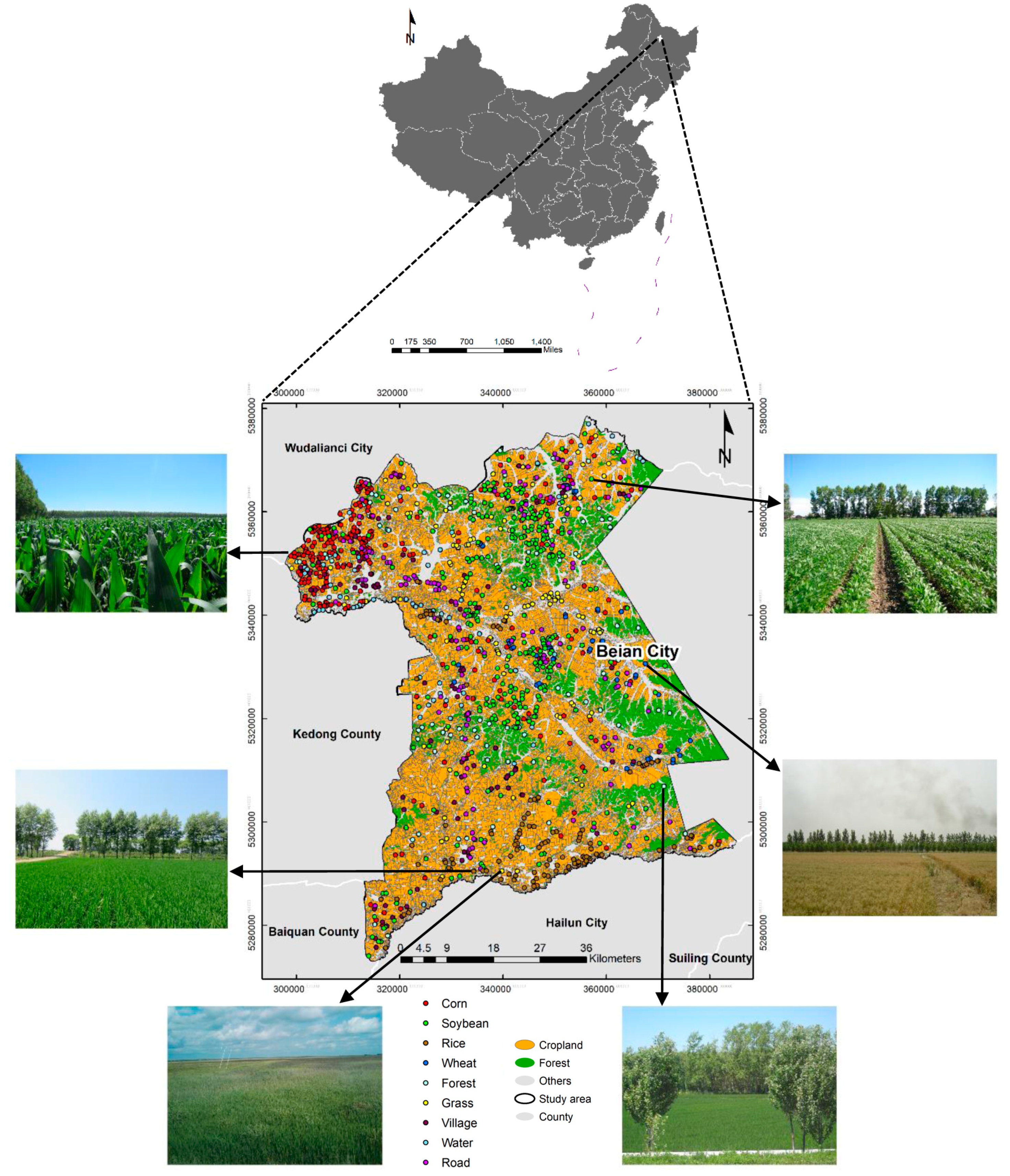
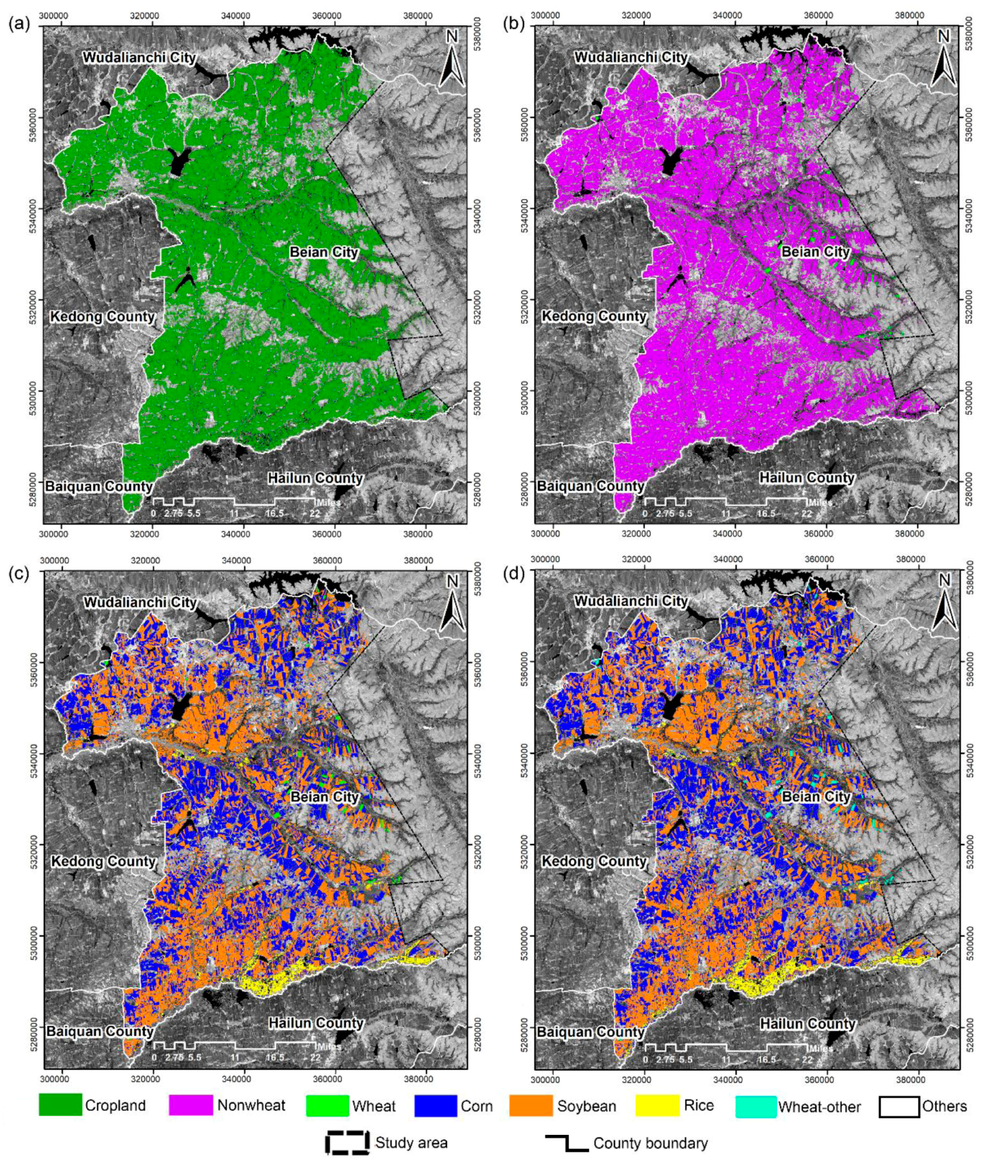
2.1 Study Area
2.2. GF-1 WFV Data
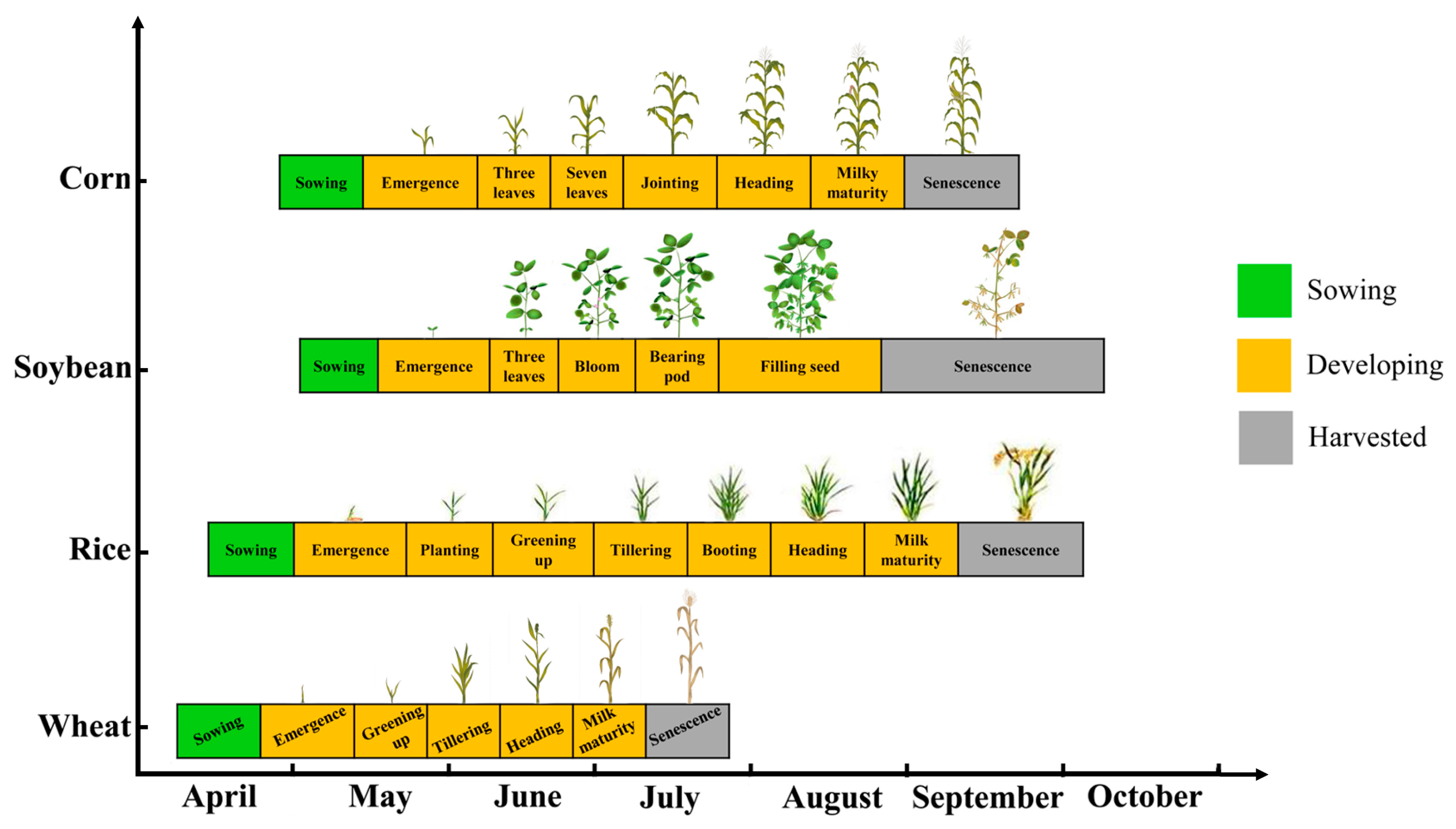
2.3. In-Season Sample Data
3. Methodology
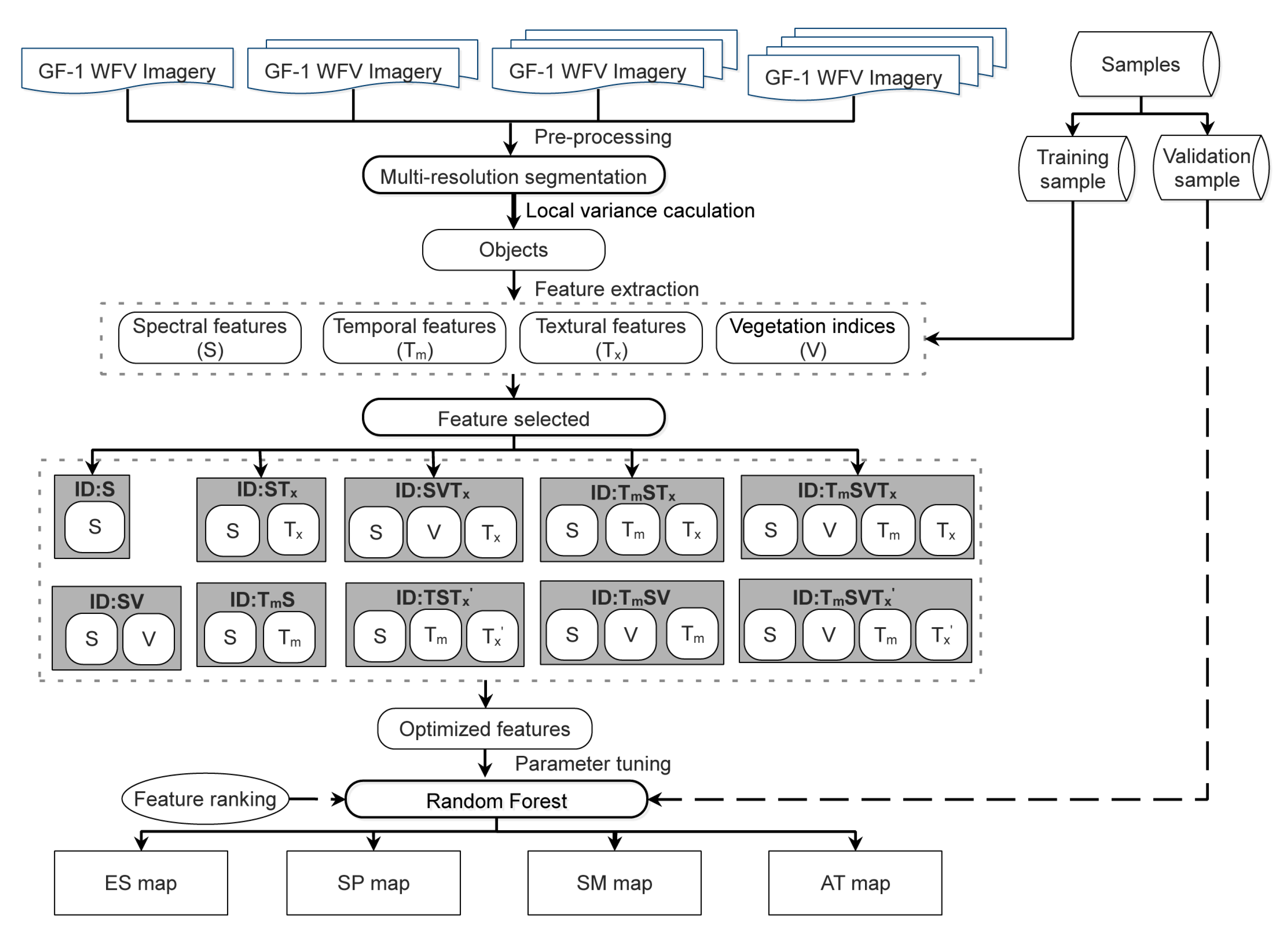
3.1. Overview of In-Season Crop Classification
- A multiresolution algorithm was used for image segmentation and the appropriate segmentation scale and the parameters associated with heterogeneity criterion were selected according to local variance;
- Evaluation on the performance of the features for different crop types according to their types (spectral reflectance, texture, temporal features and vegetation indexes);
- Analysis of the contribution of different feature types to the classification accuracy.
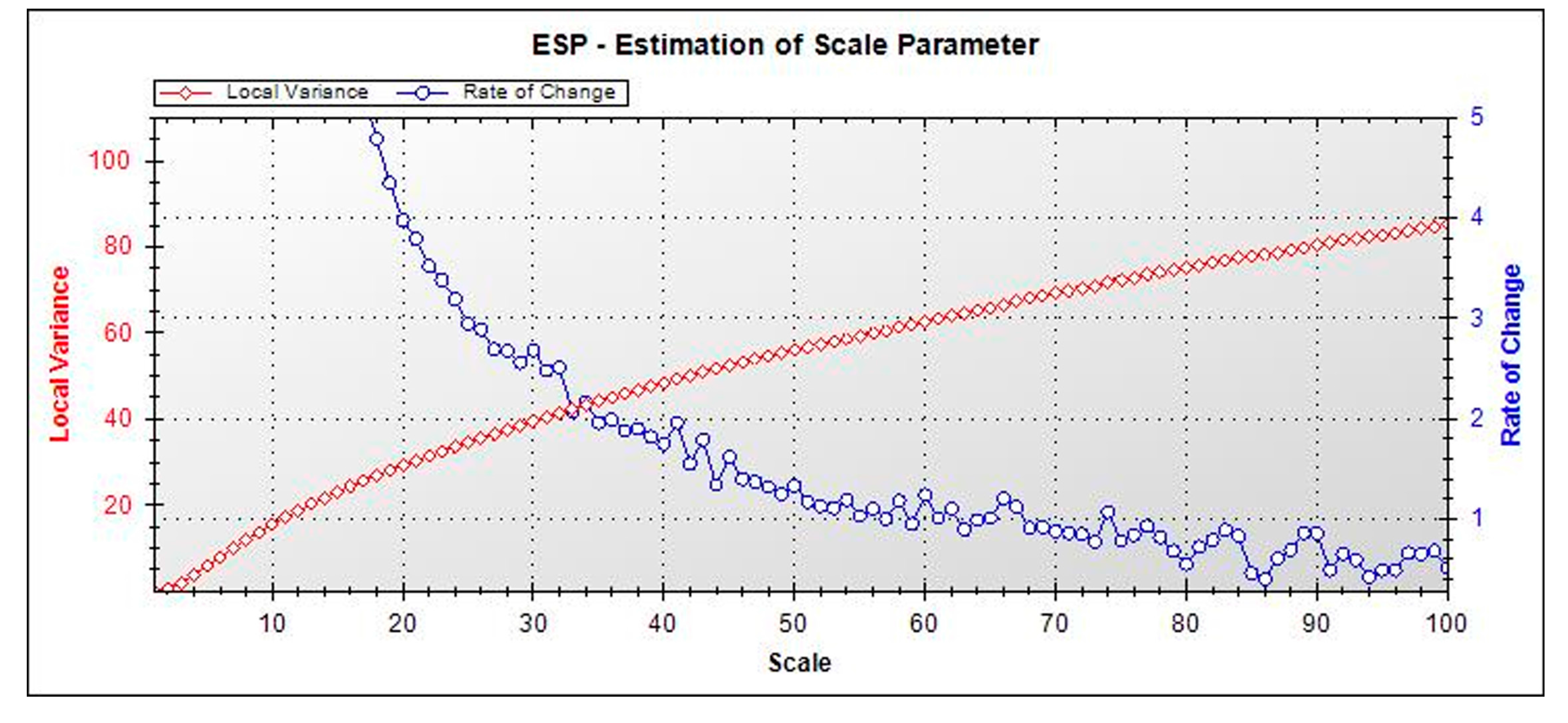
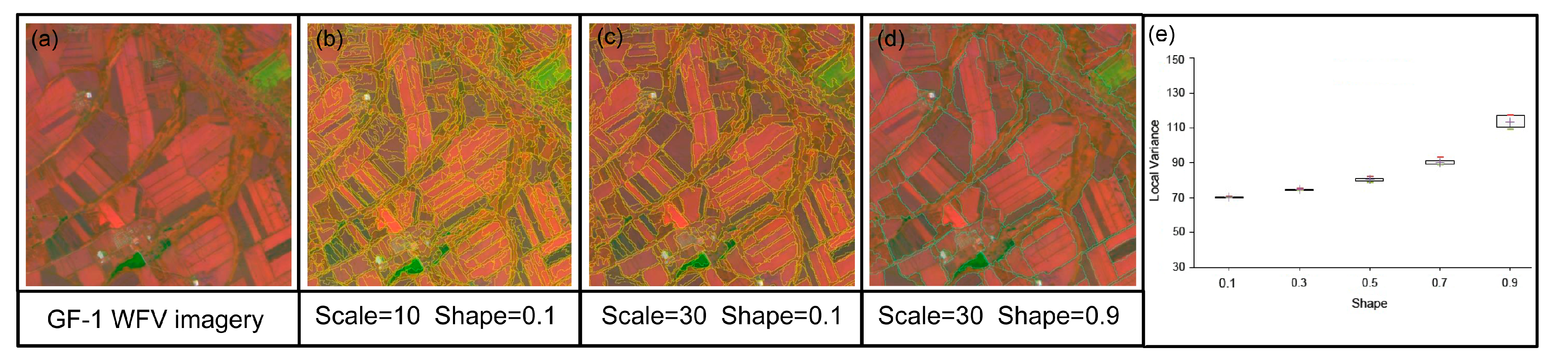
3.2. Image Segmentation
3.3. Feature Extraction
- S: The spectral features from a single image per season were taken as input. Only four available spectral bands of each scene were selected.
- STx’: The spectral bands and texture features acquired from a single image were taken as input. Four available spectral bands (4 features) and GLCM correlation, GLCM dissimilarity, and GLCM entropy from each band (12 features) acquired in specific season were selected. This experiment represents the case where spatio-spectral feature type information is employed for crop identification.
- SV: In addition to spectral features, NDVI, EVI, RVI and RI from GF-1 WFV data acquired in specific season were taken as input to enhance the spectral information. This experiment represents the case where multiple spectral information but little temporal information and non-spatial information are employed for crop identification.
- SVTx’: Along with the spatio-spectral features from a single image, vegetation indices were taken as input. This experiment represents the case where multiple spectral information but little temporal information and spatial information are employed for crop identification.
- TmS: Multi-temporal available spectral features collected during the crop present growth stages were taken as input. This experiment represents the traditional “multiple-dates” approaches. It is a case of employing multiple temporal information but little spectral information (without spectral enhancement, lack of vegetation indices) and non-spatial information for crop identification.
- TmSTx: Multi-temporal spectral and multi-temporal texture features were taken as the input. For each available date, the four bands and 12 texture features were selected. This experiment represents the cases of employing multiple spectral, multiple temporal and multiple texture information for crop identification.
- TmSTx’: Multi-temporal spectral and in-season texture features were taken as the input. Only 12 texture features were extracted from the special spectral bands acquired in present season. This experiment represents the case of employing multiple temporal, multiple spectral but little texture information to enhance the present information on crop structure and planting pattern for crop identification.
- TmSV: Multi-temporal spectral features and vegetation indices were taken as input. This experiment represents the case of employing multiple temporal information and multiple spectral information for crop identification.
- TmSVTx: The available spatio-temporal spectral and vegetation indices collected during the crop present growth stages were taken as input.
- TmSVTx’: Only the specific texture features were added into the multi-temporal spectral features and vegetation indices datasets.
3.4. Random Forest Classification
4. Results
4.1. The Optimal Segmentation Scale of Crop Type
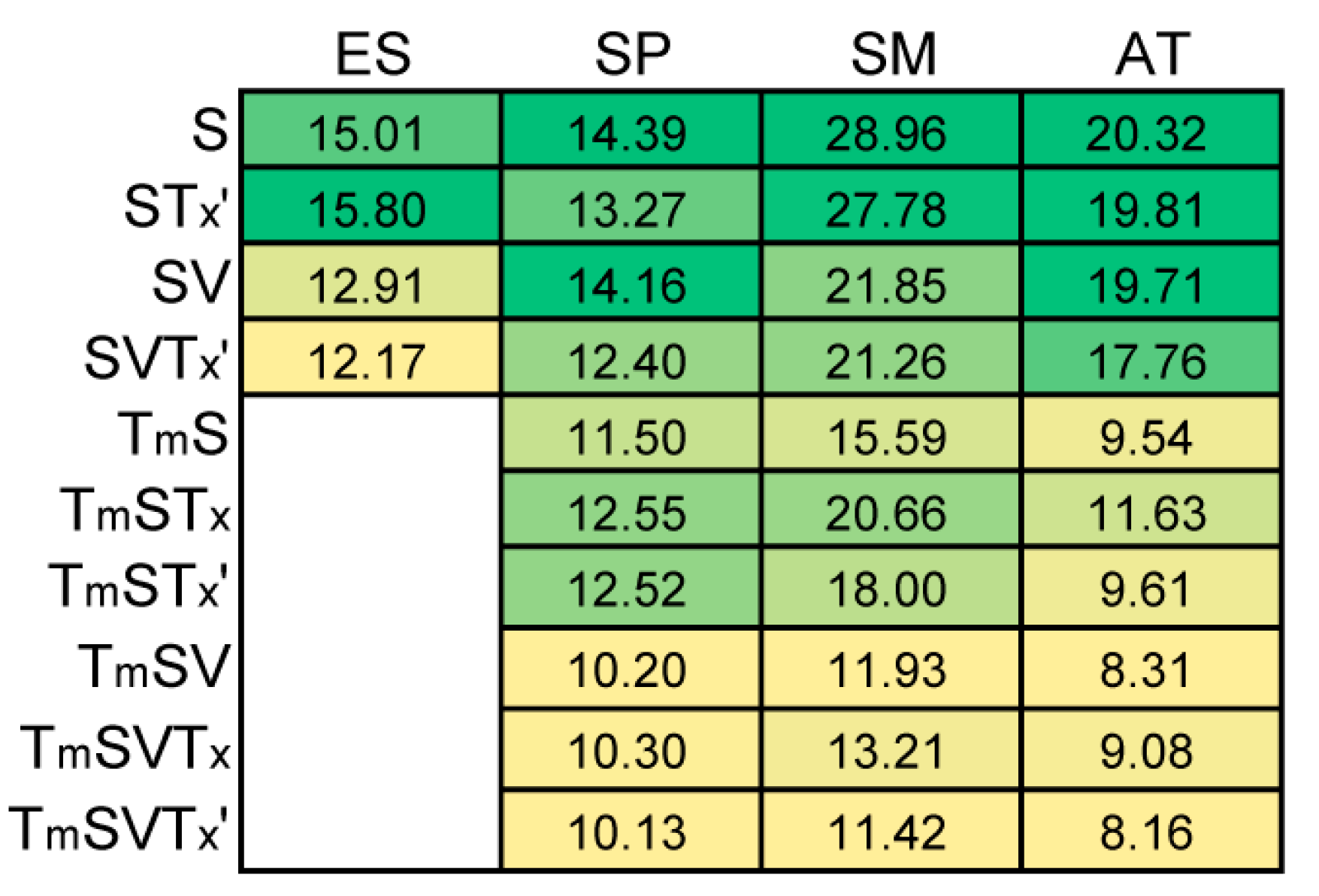
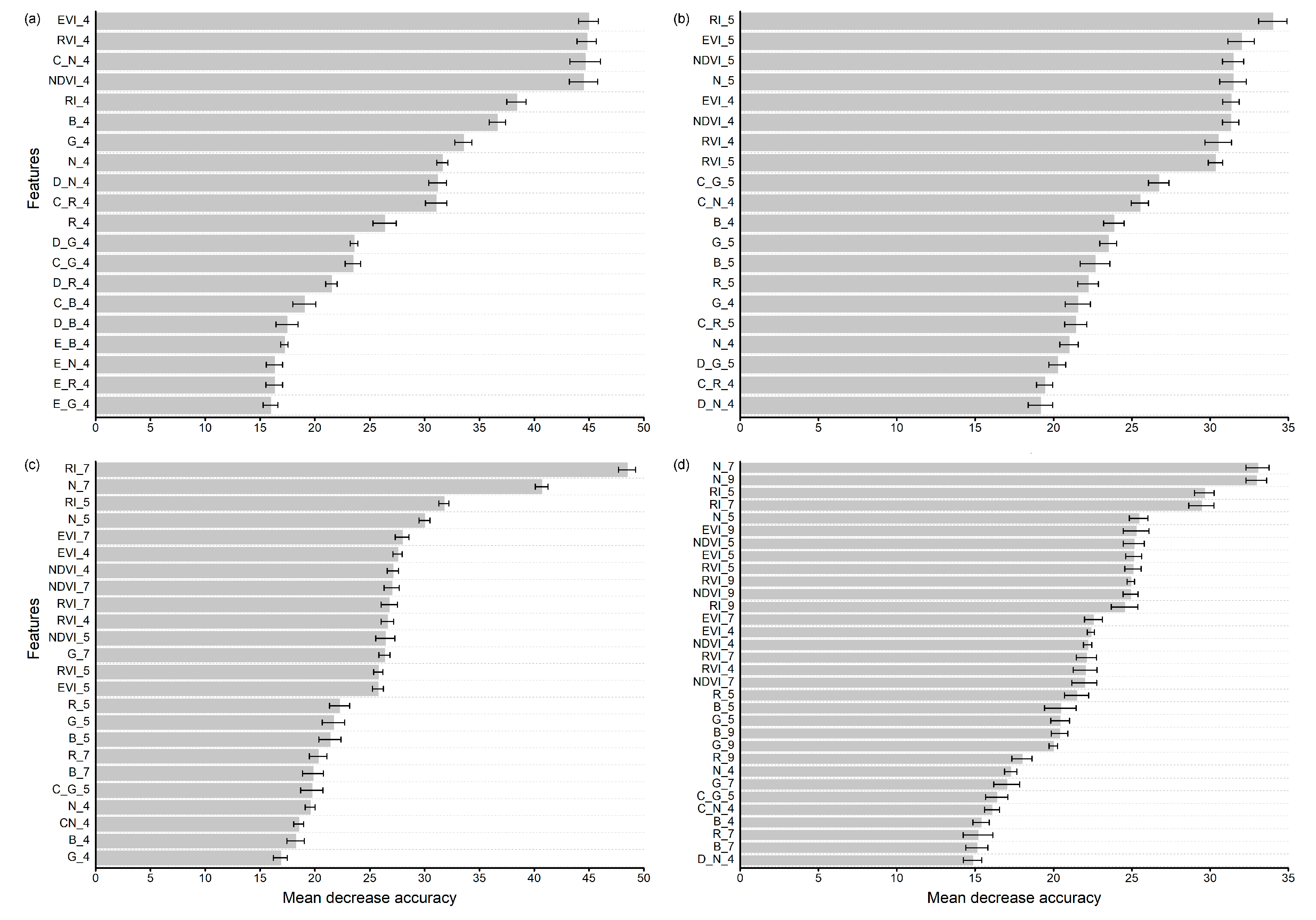
4.2. Performances of Different Feature Subspaces on Crop Classification
4.3. In-Season Crop Mapping
5. Discussion
6. Conclusions
- The map in the fourth season has the highest accuracy since it has the largest number of features and thus contains more useful information for classification. Therefore, for multiple-season crop mapping, more attention should be paid to the early seasons that may suffer from the insufficient information.
- Texture can be essential information for crop mapping when there is insufficient spectral and temporal information at the beginning of crop-growing period, whereas in-season texture helps increase the chance for mature crop classification, not only in addition to multi-temporal spectral information, but also avoiding redundancy and maximizing the classification accuracy.
- Even though we focus on the Beian City in 2014, our methods can be extended to other years for in-season crop monitoring since this robust approach possesses of the time-scale scalability. In addition, future work could address the issues on how to use multi-source finer spatial resolution data to improve the quality and timeliness of in-season crop mapping.
Acknowledgments
Author Contributions
Conflicts of Interest
References
- Mkhabela, M.; Bullock, P.; Raj, S.; Wang, S.; Yang, Y. Crop yield forecasting on the Canadian prairies using MODIS NDVI data. Agric. For. Meteorol. 2011, 151, 385–393. [Google Scholar] [CrossRef]
- Ozdogan, M. The spatial distribution of crop types from MODIS data: Temporal unmixing using independent component analysis. Remote Sens. Environ. 2010, 114, 1190–1204. [Google Scholar] [CrossRef]
- Wardlow, B.D.; Egbert, S.L.; Kastens, J.H. Analysis of time-series MODIS 250 m vegetation index data for crop classification in the U.S. Central Great Plains. Remote Sens. Environ. 2007, 108, 290–310. [Google Scholar] [CrossRef]
- Villa, P.; Bresciani, M.; Bolpagni, R.; Pinardi, M.; Giardino, C. A rule-based approach for mapping macrophyte communities using multi-temporal aquatic vegetation indices. Remote Sens. Environ. 2015, 171, 218–233. [Google Scholar] [CrossRef]
- Wu, W.B.; Yu, Q.Y.; Peter, V.H.; You, L.Z.; Yang, P.; Tang, H.J. How could agricultural land systems contribute to raise food production under global change. J. Integr. Agric. 2014, 13, 1432–1442. [Google Scholar] [CrossRef]
- Villa, P.; Stroppiana, D.; Fontanelli, G.; Azar, R.; Brivio, P. In-season mapping of crop type with optical and x-band sar data: A classification tree approach using synoptic seasonal features. Remote Sens. 2015, 7, 12859–12886. [Google Scholar] [CrossRef]
- Kontgis, C.; Schneider, A.; Ozdogan, M. Mapping rice paddy extent and intensification in the Vietnamese Mekong River Delta with dense time stacks of Landsat data. Remote Sens. Environ. 2015, 169, 255–269. [Google Scholar] [CrossRef]
- Gao, F.; Anderson, M.C.; Zhang, X.; Yang, Z.; Alfieri, J.G.; Kustas, W.P.; Mueller, R.; Johnson, D.M.; Prueger, J.H. Toward mapping crop progress at field scales through fusion of Landsat and MODIS imagery. Remote Sens. Environ. 2017, 188, 9–25. [Google Scholar] [CrossRef]
- Conrad, C.; Fritsch, S.; Zeidler, J.; Rücker, G.; Dech, S. Per-field irrigated crop classification in arid central Asia using SPOT and ASTER data. Remote Sens. 2010, 2, 1035–1056. [Google Scholar] [CrossRef] [Green Version]
- Song, X.; Potapov, P.V.; Krylov, A.; King, L.; Di Bella, C.M.; Hudson, A.; Khan, A.; Adusei, B.; Stehman, S.V.; Hansen, M.C. National-scale soybean mapping and area estimation in the United States using medium resolution satellite imagery and field survey. Remote Sens. Environ. 2017, 190, 383–395. [Google Scholar] [CrossRef]
- Singha, M.; Wu, B.F.; Zhang, M. Object-based paddy rice mapping using Hj-1A/B data and temporal features extracted from time series MODIS NDVI data. Sensors 2017, 17, 10. [Google Scholar] [CrossRef] [PubMed]
- Biradar, C.M.; Thenkabail, P.S.; Noojipady, P.; Li, Y.; Dheeravath, V.; Turral, H.; Velpuri, M.; Gumma, M.K.; Gangalakunta, O.R.P.; Cai, X.L.; et al. A global map of rainfed cropland areas (GMRCA) at the end of last millennium using remote sensing. Int. J. Appl. Earth Obs. 2009, 11, 114–129. [Google Scholar] [CrossRef]
- Pan, Y.; Li, L.; Zhang, J.; Liang, S.; Zhu, X.; Sulla-Menashe, D. Winter wheat area estimate from MODIS-EVI time series using the crop proportion phenology index. Remote Sens. Environ. 2012, 119, 232–242. [Google Scholar] [CrossRef]
- Peña-Barragán, J.M.; Ngugi, M.K.; Plant, R.E.; Six, J. Object-based crop identification using multiple vegetation indices, textural features and crop phenology. Remote Sens. Environ. 2011, 115, 1301–1316. [Google Scholar] [CrossRef]
- Fan, H.; Fu, X.; Zhang, Z.; Wu, Q. Phenology-based vegetation index differencing for mapping of rubber plantations using Landsat OLI data. Remote Sens. 2015, 7, 6041–6058. [Google Scholar] [CrossRef]
- Le, Yu; Liang, L.; Wang, J.; Zhao, Y.Y.; Cheng, Q.; Hu, L.Y.; Liu, S.; Yu, L.; Wang, X.Y.; Zhu, P.; et al. Meta-discoveries from a synthesis of satellite-based land-cover mapping research. Int. J. Remote Sens. 2014, 35, 4573–4588. [Google Scholar]
- Zhang, W.; Li, A.; Jin, H.; Bian, J.; Zhang, Z.; Lei, G.; Qin, Z.; Huang, C. An enhanced spatial and temporal data fusion model for fusing Landsat and MODIS surface reflectance to generate high temporal Landsat-like data. Remote Sens. 2013, 5, 5346–5368. [Google Scholar] [CrossRef]
- Hu, Q.; Wu, W.; Song, Q.; Lu, M.; Chen, D.; Yu, Q.; Tang, H. How do temporal and spectral features matter in crop classification. J. Integr. Agric. 2017, 16, 324–336. [Google Scholar] [CrossRef]
- Immitzer, M.; Vuolo, F.; Atzberger, C. First experience with Sentinel-2 data for crop and tree species classifications in central Europe. Remote Sens. 2016, 8, 166. [Google Scholar] [CrossRef]
- Mansaray, L.; Huang, W.; Zhang, D.; Huang, J.; Li, J. Mapping rice fields in urban Shanghai, Southeast China, using Sentinel-1a and Landsat 8 datasets. Remote Sens. 2017, 9, 257. [Google Scholar] [CrossRef]
- Jia, K.; Liang, S.L.; Gu, X.F.; Baret, F.; Wei, X.Q.; Wang, X.X.; Yao, Y.J.; Yang, L.Q.; Li, Y.W. Fractional vegetation cover estimation algorithm for Chinese GF-1 wide field view data. Remote Sens. Environ. 2016, 177, 184–191. [Google Scholar] [CrossRef]
- Song, Q.; Zhou, Q.; Wu, W.; Hu, Q.; Lu, M.; Liu, S. Mapping regional cropping patterns by using GF-1 WFV sensor data. J. Integr. Agric. 2017, 16, 337–347. [Google Scholar] [CrossRef]
- Kong, F.; Li, X.; Wang, H.; Xie, D.; Li, X.; Bai, Y. Land cover classification based on fused data from GF-1 and MODIS NDVI time series. Remote Sens. 2016, 8, 741. [Google Scholar] [CrossRef]
- Wang, Q.; Shi, W.; Li, Z.; Atkinson, P.M. Fusion of Sentinel-2 images. Remote Sens. Environ. 2016, 187, 241–252. [Google Scholar] [CrossRef]
- Lebourgeois, V.; Dupuy, S.; Vintrou, É.; Ameline, M.; Butler, S.; Bégué, A. A combined random forest and OBIA classification scheme for mapping smallholder agriculture at different nomenclature levels using multisource data (simulated Sentinel-2 time series, VHRS and DEM). Remote Sens. 2017, 9, 259. [Google Scholar] [CrossRef]
- Wu, M.; Zhang, X.; Huang, W.; Niu, Z.; Wang, C.; Li, W.; Hao, P. Reconstruction of daily 30 m data from HJ CCD, GF-1 WFV, Landsat, and MODIS data for crop monitoring. Remote Sens. 2015, 7, 16293–16314. [Google Scholar] [CrossRef]
- Hu, Q.; Wu, W.B.; Xia, T.; Yu, Q.Y.; Yang, P.; Li, Z.G.; Song, Q. Exploring the use of google earth imagery and object-based methods in land use/cover mapping. Remote Sens. 2013, 5, 6026–6042. [Google Scholar] [CrossRef]
- Li, Q.; Wang, C.; Zhang, B.; Lu, L. Object-based crop classification with Landsat-MODIS enhanced time-series data. Remote Sens. 2015, 7, 16091–16107. [Google Scholar] [CrossRef]
- Costa, H.; Carrão, H.; Bação, F.; Caetano, M. Combining per-pixel and object-based classifications for mapping land cover over large areas. Int. J. Remote Sens. 2014, 35, 738–753. [Google Scholar] [CrossRef]
- Han, N.; Du, H.; Zhou, G.; Sun, X.; Ge, H.; Xu, X. Object-based classification using SPOT-5 imagery for Moso bamboo forest mapping. Int. J. Remote Sens. 2014, 35, 1126–1142. [Google Scholar] [CrossRef]
- Castillejo-González, I.L.; López-Granados, F.; García-Ferrer, A.; Peña-Barragán, J.M.; Jurado-Expósito, M.; de la Orden, M.S.; González-Audicana, M. Object- and pixel-based analysis for mapping crops and their agro-environmental associated measures using QuickBird imagery. Comput. Electron. Agric. 2009, 68, 207–215. [Google Scholar] [CrossRef]
- Ursani, A.A.; Kpalma, K.; Lelong, C.C.D.; Ronsin, J. Fusion of textural and spectral information for tree crop and other agricultural cover mapping with very-high resolution satellite images. IEEE J. Sel. Top. Appl. Earth Obs. 2012, 5, 225–235. [Google Scholar] [CrossRef]
- Zhang, H.X.; Li, Q.Z.; Liu, J.G.; Du, X.; Dong, T.F.; McNairn, H.; Champagne., C.; Liu, M.X.; Shang, J.L. Object-based crop classification using multi- temporal SPOT-5 imagery and textural features with a random forest classifier. Geocarto Int. 2017, 1–19. [Google Scholar] [CrossRef]
- Breiman, L. Random forests. Mach. Learn. 2001, 45, 5–32. [Google Scholar] [CrossRef]
- Mathur, A.; Foody, G.M. Crop classification by support vector machine with intelligently selected training data for an operational application. Int. J. Remote Sens. 2008, 29, 2227–2240. [Google Scholar] [CrossRef]
- Tatsumi, K.; Yamashiki, Y.; Canales Torres, M.A.; Taipe, C.L.R. Crop classification of upland fields using Random forest of time-series Landsat 7 ETM+ data. Comput. Electron. Agric. 2015, 115, 171–179. [Google Scholar] [CrossRef]
- Ok, A.O.; Akar, O.; Gungor, O. Evaluation of random forest method for agricultural crop classification. Eur. J. Remote Sens. 2012, 45, 421–432. [Google Scholar] [CrossRef]
- Fletcher, R.S. Using vegetation indices as input into random forest for soybean and weed classification. Am. J. Plant Sci. 2016, 7, 2186–2198. [Google Scholar] [CrossRef]
- Sonobe, R.; Tani, H.; Wang, X.; Kobayashi, N.; Shimamura, H. Parameter tuning in the support vector machine and random forest and their performances in cross- and same-year crop classification using TerraSAR-X. Int. J. Remote Sens. 2012, 35, 260–267. [Google Scholar] [CrossRef]
- Duro, D.C.; Franklin, S.E.; Dubé, M.G. A comparison of pixel-based and object-based image analysis with selected machine learning algorithms for the classification of agricultural landscapes using SPOT-5 HRG imagery. Remote Sens. Environ. 2012, 118, 259–272. [Google Scholar] [CrossRef]
- Duro, D.C.; Franklin, S.E.; Dubé, M.G. Multi-scale object-based image analysis and feature selection of multi-sensor earth observation imagery using random forests. Int. J. Remote Sens. 2012, 33, 4502–4526. [Google Scholar] [CrossRef]
- Vieira, M.A.; Formaggio, A.R.; Rennó, C.D.; Atzberger, C.; Aguiar, D.A.; Mello, M.P. Object based image analysis and data mining applied to a remotely sensed Landsat time-series to map sugarcane over large areas. Remote Sens. Environ. 2012, 123, 553–562. [Google Scholar] [CrossRef]
- Bureau, H.S. Heilongjiang Statistic Yearbook; Bureau of Heilongjiang Statistic: Harbin, China, 2015.
- China Centre for Resources Satellite Data and Application. Available online: http://www.cresda.com/CN/ (accessed on 17 December 2014).
- Baatz, M.; Schäpe, A. Multiresolution segmentation: An optimization approach for high quality multi-scale image segmentation. J. Photogramm. Remote Sens. 2000, 58, 12–23. [Google Scholar]
- Mathieu, R.; Aryal, J.; Chong, A.K. Object-based classification of Ikonos imagery for mapping large-scale vegetation communities in urban areas. Sensors 2007, 7, 2860–2880. [Google Scholar] [CrossRef] [PubMed]
- Drǎguţ, L.; Tiede, D.; Levick, S.R. ESP: A tool to estimate scale parameter for multiresolution image segmentation of remotely sensed data. Int. J. Geogr. Inf. Sci. 2010, 24, 859–871. [Google Scholar] [CrossRef]
- Jia, K.; Wu, B.; Li, Q. Crop classification using HJ satellite multispectral data in the North China Plain. J. Appl. Remote Sens. 2013, 7, 073576. [Google Scholar] [CrossRef]
- Zhong, L.; Gong, P.; Biging, G.S. Efficient corn and soybean mapping with temporal extendability: A multi-year experiment using Landsat imagery. Remote Sens. Environ. 2014, 140, 1–13. [Google Scholar] [CrossRef]
- Patil, A.; Lalitha, Y.S. Classification of crops using FCM segmentation and texture, color feature. Int. J. Adv. Res. Comput. Commun. Eng. 2012, 1, 371–377. [Google Scholar]
- Gao, T.; Zhu, J.; Zheng, X.; Shang, G.; Huang, L.; Wu, S. Mapping spatial distribution of larch plantations from multi-seasonal Landsat-8 OLI imagery and multi-scale textures using Random Forests. Remote Sens. 2015, 7, 1702–1720. [Google Scholar] [CrossRef]
- Pelletier, C.; Valero, S.; Inglada, J.; Champion, N.; Dedieu, G. Assessing the robustness of Random Forests to map land cover with high resolution satellite image time series over large areas. Remote Sens. Environ. 2016, 187, 156–168. [Google Scholar] [CrossRef]
- Peña, M.A.; Brenning, A. Assessing fruit-tree crop classification from Landsat-8 time series for the Maipo Valley, Chile. Remote Sens. Environ. 2015, 171, 234–244. [Google Scholar] [CrossRef]
- Loosvelt, L.; Peters, J.; Skriver, H.; Lievens, H.; Coillie, F. Random forests as a tool for estimating uncertainty at pixel-level in SAR image classification. Int. J. Appl. Earth Obs. 2012, 19, 173–184. [Google Scholar] [CrossRef]
- Maus, V.; Camara, G.; Cartaxo, R.; Sanchez, A.; Ramos, F.M. A time-weighted dynamic time warping method for land-use and land-cover mapping. IEEE J. Sel. Top. Appl. Earth Obs. 2016, 9, 1–11. [Google Scholar] [CrossRef]
- Petitjean, F.; Inglada, J.; Gancarski, P. Satellite image time series analysis under time warping. IEEE Trans. Geosci. Remote Sens. 2012, 50, 3081–3095. [Google Scholar] [CrossRef]
- Petitjean, F.; Kurtz, C.; Passat, N.; Arski, P.G. Spatio-temporal reasoning for the classification of satellite image time series. Pattern Recogn. Lett. 2012, 33, 1805–1815. [Google Scholar] [CrossRef]
- Waldner, F.; Canto, G.S.; Defourny, P. Automated annual cropland mapping using knowledge-based temporal features. ISPRS J. Photogramm. Remote Sens. 2015, 110, 1–13. [Google Scholar] [CrossRef]
- Yan, L.; Roy, D.P. Automated crop field extraction from multi-temporal web enabled Landsat data. Remote Sens. Environ. 2014, 114, 42–64. [Google Scholar] [CrossRef]
- Böck, S.; Immitzer, M.; Atzberger, C. On the objectivity of the objective function–problems with unsupervised segmentation evaluation based on global score and a possible remedy. Remote Sens. 2017, 9, 769. [Google Scholar] [CrossRef]


| Survey Date | Crop Types | Samples | Training Samples | Validation Samples |
|---|---|---|---|---|
| 20 April | Cropland | 1121 | 789 | 332 |
| Others | 656 | 516 | 140 | |
| 20 May | Wheat | 68 | 53 | 15 |
| Non-wheat | 1053 | 736 | 317 | |
| Others | 656 | 516 | 140 | |
| 20 July | Corn | 415 | 275 | 140 |
| Soybean | 474 | 334 | 140 | |
| Rice | 164 | 126 | 38 | |
| Wheat | 68 | 53 | 15 | |
| Others | 656 | 516 | 140 | |
| 20 September | Corn | 415 | 275 | 140 |
| Soybean | 474 | 334 | 140 | |
| Rice | 164 | 126 | 38 | |
| Wheat-other | 68 | 53 | 15 | |
| Others | 656 | 516 | 140 |
| In-Season ID | Period of Mapping | Targeted Types |
|---|---|---|
| ES | Early spring | Cropland/Others |
| SP | Spring | Non-wheat/Wheat/Others |
| SM | Summer | Corn/Soybean/Rice/Wheat/Others |
| AT | Autumn | Corn/Soybean/Rice/Wheat-other/Others |
| Feature Scenario | ES | SP | SM | AT | ||||||||||||
|---|---|---|---|---|---|---|---|---|---|---|---|---|---|---|---|---|
| S | Tm | Tx | V | S | Tm | Tx | V | S | Tm | Tx | V | S | Tm | Tx | V | |
| S | 4 | 4 | 4 | 4 | ||||||||||||
| STx’ | 4 | 12 | 4 | 12 | 4 | 12 | 4 | 12 | ||||||||
| SV | 4 | 4 | 4 | 4 | 4 | 4 | 4 | 4 | ||||||||
| SVTx’ | 4 | 12 | 4 | 4 | 12 | 4 | 4 | 12 | 4 | 4 | 12 | 4 | ||||
| TmS | 8 | 2 | 12 | 3 | 16 | 4 | ||||||||||
| TmSTx | 8 | 2 | 24 | 12 | 3 | 36 | 16 | 4 | 48 | |||||||
| TmSTx’ | 8 | 2 | 12 | 12 | 3 | 12 | 16 | 4 | 12 | |||||||
| TmSV | 8 | 2 | 8 | 12 | 3 | 12 | 16 | 4 | 16 | |||||||
| TmSVTx | 8 | 2 | 24 | 8 | 12 | 3 | 36 | 12 | 16 | 4 | 48 | 16 | ||||
| TmSVTx’ | 8 | 2 | 12 | 8 | 12 | 3 | 12 | 12 | 16 | 4 | 12 | 16 | ||||
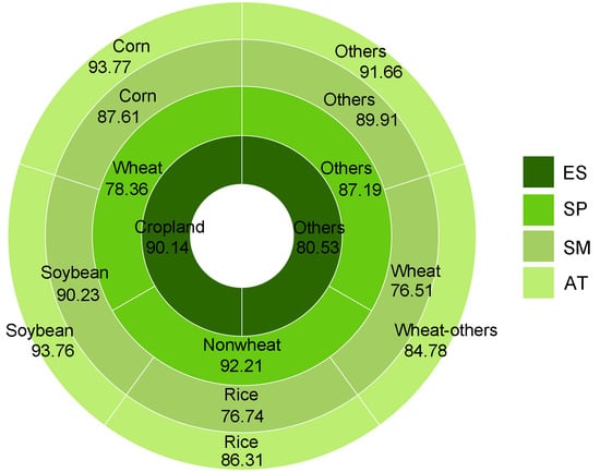
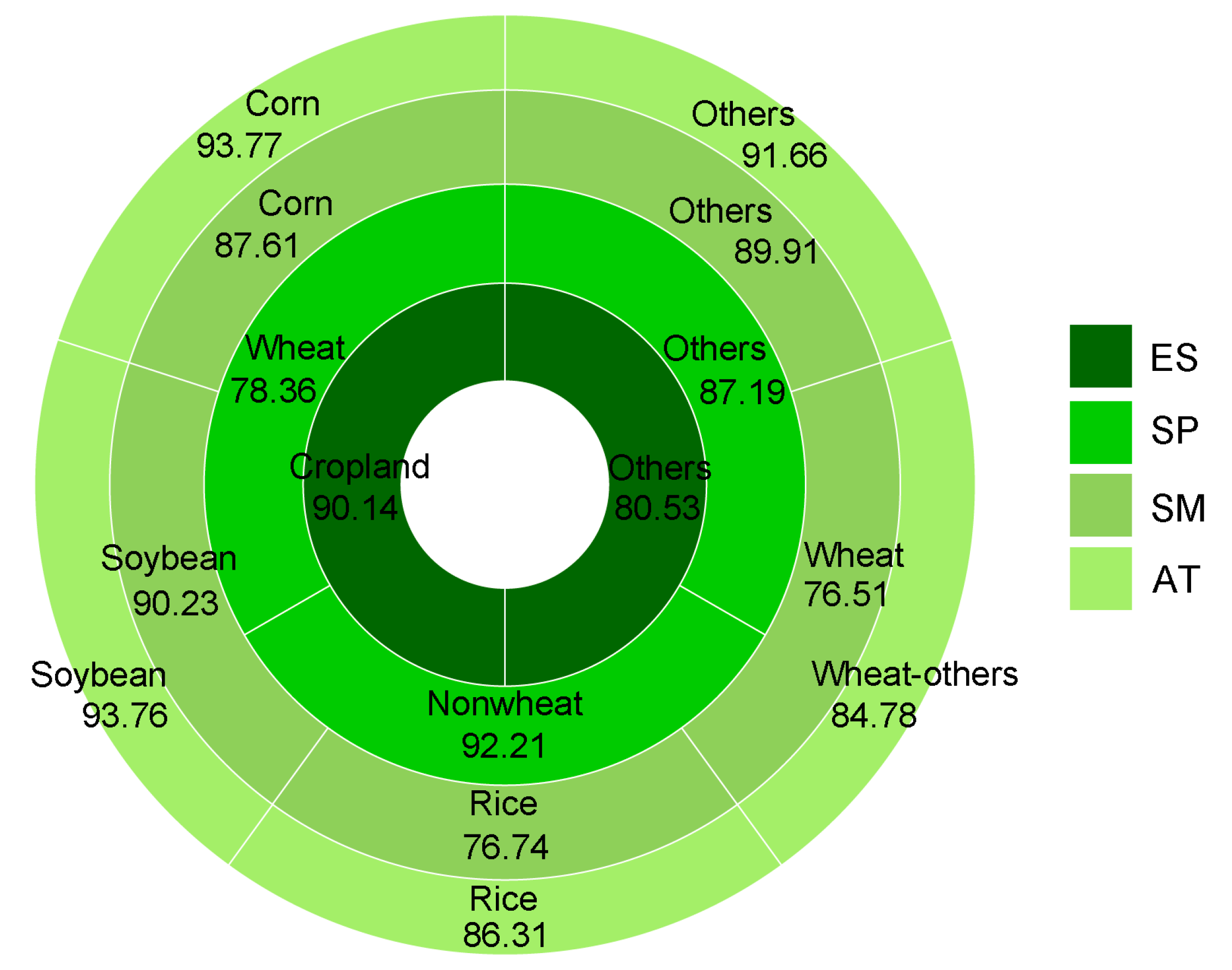
| Season ID | Classification Type | UA (%) | PA (%) |
| ES | Cropland | 90.86 | 89.05 |
| Others | 82.95 | 85.60 | |
| Overall accuracy = 87.73% Kappa coefficient = 0.7421 | |||
| Season ID | Classification Type | UA (%) | PA (%) |
| SP | Non-wheat | 92.38 | 92.44 |
| Wheat | 66.04 | 97.22 | |
| Others | 88.76 | 86.09 | |
| Overall accuracy = 91.26% Kappa coefficient = 0.8263 | |||
| Season ID | Classification Type | UA (%) | PA (%) |
| SM | Corn | 85.81 | 89.39 |
| Soybean | 89.22 | 90.85 | |
| Rice | 77.98 | 78.23 | |
| Wheat | 64.15 | 97.14 | |
| Others | 93.21 | 86.98 | |
| Overall accuracy = 87.88% Kappa coefficient = 0.8305 | |||
| Season ID | Classification Type | UA (%) | PA (%) |
| AT | Corn | 90.55 | 97.65 |
| Soybean | 94.01 | 93.18 | |
| Rice | 81.75 | 91.15 | |
| Wheat-others | 73.59 | 95.12 | |
| Others | 95.54 | 87.99 | |
| Overall accuracy = 91.72% Kappa coefficient = 0.8839 | |||
© 2017 by the authors. Licensee MDPI, Basel, Switzerland. This article is an open access article distributed under the terms and conditions of the Creative Commons Attribution (CC BY) license (http://creativecommons.org/licenses/by/4.0/).
Share and Cite
Song, Q.; Hu, Q.; Zhou, Q.; Hovis, C.; Xiang, M.; Tang, H.; Wu, W. In-Season Crop Mapping with GF-1/WFV Data by Combining Object-Based Image Analysis and Random Forest. Remote Sens. 2017, 9, 1184. https://0-doi-org.brum.beds.ac.uk/10.3390/rs9111184
Song Q, Hu Q, Zhou Q, Hovis C, Xiang M, Tang H, Wu W. In-Season Crop Mapping with GF-1/WFV Data by Combining Object-Based Image Analysis and Random Forest. Remote Sensing. 2017; 9(11):1184. https://0-doi-org.brum.beds.ac.uk/10.3390/rs9111184
Chicago/Turabian StyleSong, Qian, Qiong Hu, Qingbo Zhou, Ciara Hovis, Mingtao Xiang, Huajun Tang, and Wenbin Wu. 2017. "In-Season Crop Mapping with GF-1/WFV Data by Combining Object-Based Image Analysis and Random Forest" Remote Sensing 9, no. 11: 1184. https://0-doi-org.brum.beds.ac.uk/10.3390/rs9111184