Hyperspectral Super-Resolution with Spectral Unmixing Constraints

Abstract

Hyperspectral sensors capture a portion of the visible and near-infrared spectrum with many narrow spectral bands. This makes it possible to better discriminate objects based on their reflectance spectra and to derive more detailed object properties. For technical reasons, the high spectral resolution comes at the cost of lower spatial resolution. To mitigate that problem, one may combine such images with conventional multispectral images of higher spatial, but lower spectral resolution. The process of fusing the two types of imagery into a product with both high spatial and spectral resolution is called hyperspectral super-resolution. We propose a method that performs hyperspectral super-resolution by jointly unmixing the two input images into pure reflectance spectra of the observed materials, along with the associated mixing coefficients. Joint super-resolution and unmixing is solved by a coupled matrix factorization, taking into account several useful physical constraints. The formulation also includes adaptive spatial regularization to exploit local geometric information from the multispectral image. Moreover, we estimate the relative spatial and spectral responses of the two sensors from the data. That information is required for the super-resolution, but often at most approximately known for real-world images. In experiments with five public datasets, we show that the proposed approach delivers up to 15% improved hyperspectral super-resolution.

1. Introduction

Hyperspectral imaging, also called imaging spectroscopy, delivers image data with many (up to several hundreds) contiguous spectral bands of narrow bandwidth, on the order of a few nm. The spectral range depends on the sensor; typically it covers the visible wavelengths and some part of the near-infrared region, up to at most 2.5 µm. With hyperspectral sensors (also known as imaging spectrometers), one can more accurately distinguish visually similar surface materials, since every material has its own, characteristic reflectance spectrum. For our purposes, we in fact identify a “material” with a unique reflectance spectrum. Without reference spectra, one cannot separate two physically-different surface compounds if they always occur together in fixed proportions. Based on these spectra, one can not only detect and localize more different objects, e.g., for land cover mapping, environmental and agricultural monitoring; one can also estimate further (bio-)physical and (bio-)chemical properties. For a discussion of important applications, see, e.g., [1]. However, as a consequence of the very narrow spectral bands, only a small amount of radiant energy is available in each band. To achieve an acceptable signal-to-noise ratio (SNR), the sensor area per pixel must therefore be large, leading to coarser geometric resolution. This is the opposite situation of multispectral cameras, where much of the spectral information is sacrificed to achieve high spatial resolution, by integrating the scene radiance over fewer, much wider spectral bands.

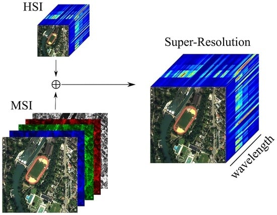
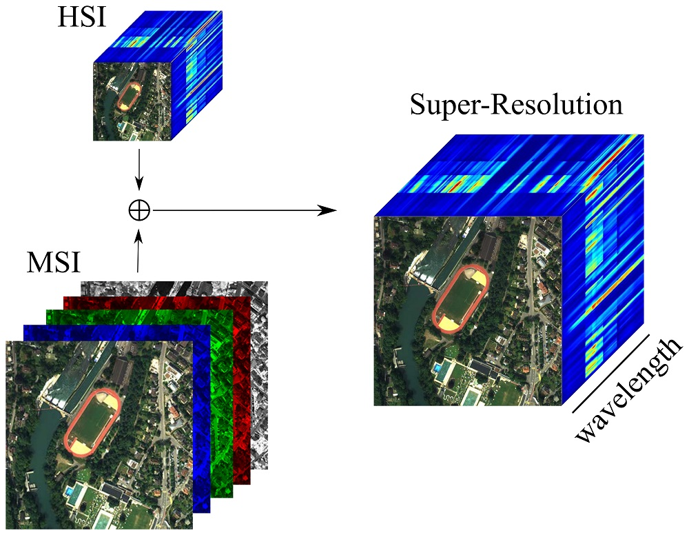
To get the best of both worlds, a natural possibility is to fuse a hyperspectral image (termed HSI in the following) with a multispectral image (termed MSI), resulting in a synthetic image with both high spectral and spatial resolution; see Figure 1. This process is referred to as hyperspectral super-resolution or hyperspectral and multispectral data fusion. For a recent overview, see [2].

A starting point for this work is the observation that hyperspectral super-resolution is linked to the well-known problem of spectral unmixing: pixels in the HSI, having a larger footprint on the ground, often include a mixture of multiple materials. The aim of unmixing is to determine, at each pixel, the observed pure material spectra (endmembers) and their proportions (abundances). When increasing the resolution, there will be fewer mixed pixels; at the same time, the endmembers and abundances should be preserved.

We follow the classical, linear spectral mixing model [3]. Inspired by it, we formulate super-resolution as a factorization of the image data into a (non-orthogonal) basis of endmembers, and the corresponding coefficients to represent the data in that basis, which can be interpreted as fractional abundances. Unmixing imposes physical constraints: in particular, neither the reflected intensity at any wavelength, nor the surface area covered by a material can ever be negative, and each observed spectrum should be completely described by a mixture of few materials. In our work, we impose the necessary constraints to ensure a physically-plausible unmixing. We point out that this does not guarantee physically correct, pure material spectra: the latter cannot be found from the data alone. Still, we will, in line with the literature, use the terms endmembers and abundances. Technically, we cast the super-resolution as a coupled, constrained matrix factorization of the two input images into their mutually-dependent endmembers and abundances. That is, we constrain the problem as tightly as possible under the linear mixing model, thus removing slack that could potentially help to absorb non-linear effects. Still, we find that the linear approximation holds sufficiently well, such that the added stability outweighs the reduced flexibility. Our formulation delivers improved fusion results, as well as a visually convincing segmentation into spectrally-distinct materials.

To relate am MSI and HSI of the same scene, one needs the (relative) spatial and spectral responses of the two sensors. Most existing work assumes that these responses are known in advance. However, in practice, this is not always the case. On the one hand, the sensor specifications may be (partially) unknown. On the other hand, the specifications determined in the laboratory may differ from the actual behavior during deployment, particularly in orbit, e.g., due to aging and deterioration of sensor components or malfunctioning of on-board calibration devices [4]. In actual fact, the overwhelming majority of experiments in hyperspectral super-resolution have so far used synthetic data, since it is otherwise very hard to generate high-quality reference data. When the input HSI and MSI are generated by synthetically degrading an existing image, the spatial and spectral response functions are known, by definition. We aim for a method that can be applied in most practical situations; therefore, we also propose methods to derive the relative spatial and spectral sensor responses directly from the data, given approximately co-registered HSI and MSI. Again, we ensure plausible (non-negative) responses, which significantly stabilizes the estimation. We note that the center of the response function is part of the relative spatial response. By estimating its remaining translation, we can correct co-registration errors, which is rather useful in practice, since sub-pixel accurate co-registration between images from different sources can be challenging.

Here, we also extend an earlier, preliminary version of our method [5] to include an adaptive spatial regularizer. It is generally accepted that, in natural images, nearby pixel values are correlated. These spatial correlations, particularly in the high-resolution MSI, potentially contain much information that can be used to regularize the result. Hence, we include in our model a quadratic smoothing term, modulated by the edges (gradients) of the MSI, to favor spatially-smooth outputs.

Overall, our proposed method features (i) physically-constrained hyperspectral super-resolution including (ii) spatial regularization and (iii) data-driven recovery of the necessary relative spatial and spectral response functions. In reference to the underlying mathematical optimization technique, we call our method SupResPALM (super-resolution with proximal alternating linearized minimization).

2. Related Work

The limitation that hyperspectral images can only be acquired at low spatial resolution has naturally led researchers in remote sensing and computer vision to try and fuse them with high-resolution multispectral or panchromatic images. From the point of view of image processing, the problem is a special case of image fusion [6]. Perhaps the most widespread use of image fusion in remote sensing is pan-sharpening with a single, pan-chromatic high-resolution image. That method has also been applied to hyperspectral images, for a recent review, see [7]. However, hyperspectral super-resolution is more general, in that the high-resolution input may have multiple (possibly overlapping) spectral bands.

Our work is closely related to methods that rely on a linear basis (linear unmixing) and some type of matrix factorization. Kawakami et al. [8] first learn a fixed spectral basis by unmixing the HSI via ${\mathit{l}}_1$-minimization. Then, using this basis, they compute mixing coefficients for the MSI (here RGB) pixels, using ${\mathit{l}}_1$-minimization to encourage sparsity. Huang et al. [9] learn the spectral basis with SVD and solve for the MSI mixing coefficients with orthogonal matching pursuit (OMP). Akhtar et al. [10] learn a non-negative spectral basis from the HSI, and then solve for the MSI coefficients under a sparsity constraint, again using OMP. Simões et al. [11] also recover a linear basis, and include a total variation regularizer to achieve spatial smoothness of the mixing coefficients. Like the previously mentioned works, they proceed sequentially and first construct a basis, which is then held fixed to solve for the coefficients in a second step.

On the contrary, Yokoya et al. [12] also update the spectral basis. They ensure that the mixing coefficients are ≥0, by unmixing both the HSI and the MSI in an iterative fashion, with non-negative matrix factorization. Wycoff et al. [13] also use a joint energy function for both the basis and the coefficients, which supports sparsity and non-negativity. Veganzones et al. [14] propose an approach to handle the case where the intrinsic dimensionality of the HSI is large, by exploiting that, even then, the local subspace in a small neighborhood is often low-dimensional. [15,16] allow for priors on the distribution of image intensities and do MAP inference, which, for simple priors, is equivalent to reweighting the contributions of pixels to the error function. Wei et al. [17] have proposed an efficient Bayesian model, in which maximizing the likelihood corresponds to solving a Sylvester equation. That work has then been generalized [18], to be more robust with respect to the blur kernel, and also slightly more efficient. Recently, Zou and Xia [19] use an instance of non-negative factorization to compute endmembers and abundances with graph Laplacian regularization, without however making use of the sum-to-one constraint.

In our work, we also rely on the factorization of a linear mixture model, but attempt to base the super-resolution on an optimal, physically-plausible reconstruction of the endmembers and their abundances. While most state-of-the-art work uses some of the constraints that arise from the elementary physics of spectral mixing, only our model and very recent, concurrent work by Wei et al. [20] use all of them. The formulation of Wei et al. [20] leads to an alternating optimization of fusion and unmixing, with Sylvester equation solvers; whereas we use efficient proximal mappings to impose the constraints. Moreover, to account for the influence of the constraints on the spectral basis, we update the endmembers together with the abundances, whereas [8,9,10,11,21] estimate the spectral basis in advance and then keep it fixed. Finally, while several other methods include some sort of smoothness prior, e.g., vector total variation in [11], or the $L_2$-distance to the bicubic upsampling in [17], we are not aware of any prior work that uses the MSI to obtain an adaptive regularizer.

There is not much literature about the estimation of relative MSI/HSI sensor responses. To the best of our knowledge, the issue has been investigated only as a prerequisite for hyperspectral super-resolution. Yokoya et al. [22] assume perfect co-registration and model the spatial response as a zero-mean Gaussian blur, whose variance is estimated by maximizing the cross-correlation between the HSI and downsampled-MSI gradients. They strongly constrain the spectral response to deviate only slightly from the known laboratory values. Huang et al. [9] propose an unconstrained solution for the spectral response, which however does not appear to yield plausible results [22]. Finally, Simões et al. [11] estimate both responses, assuming that the width of the MSI spectral response is known. Both response functions are regularized by quadratic regularization of the gradient, which in our experience tends to over-smooth. Furthermore, non-negativity of the response is not enforced.

3. Problem Formulation

We are searching for an image $\overline{\mathbf{Z}}\in {\mathbb{R}}^{W\times H\times B}$ that has both high spatial and high spectral resolution, with W, H and B the image width, image height and number of spectral bands respectively. For that task, we have two inputs: a hyperspectral image $\overline{\mathbf{H}}\in {\mathbb{R}}^{w\times h\times B}$ with (much) lower spatial resolution, i.e., the same region in object space is covered by a smaller number of pixels: $w\ll W$ and $h\ll H$; and a multispectral image $\overline{\mathbf{M}}\in {\mathbb{R}}^{W\times H\times b}$ with high spatial resolution, but a reduced number of spectral bands, $b\ll B$.

To simplify the notation, we will write images as matrices. That is, all pixels of an image are concatenated, such that every column of the matrix corresponds to the spectral responses at a given pixel, and every row corresponds to a specific spectral band of the complete image. Accordingly, the images are written $\mathbf{Z}\in {\mathbb{R}}^{B\times N_m}$, $\mathbf{H}\in {\mathbb{R}}^{B\times N_h}$ and $\mathbf{M}\in {\mathbb{R}}^{b\times N_m}$, where $N_h=wh$ and $N_m=WH$.

In the linear mixing model [3,23], the intensities $\mathbf{z}\in {\mathbb{R}}^B$ at a given pixel i of $\mathbf{Z}$ are described by an additive mixture:

$${\mathbf{z}}_i=\sum _{j=1}^p{\mathbf{e}}_j{a}_{ij},\mathbf{Z}=\mathbf{E}\mathbf{A},$$

(1)

with a matrix $\mathbf{E}\equiv [{\mathbf{e}}_1,{\mathbf{e}}_2,\dots ,{\mathbf{e}}_p]$ of pure spectra (endmembers) a matrix $\mathbf{A}\equiv [{\mathbf{a}}_1,{\mathbf{a}}_2,\dots ,{\mathbf{a}}_{N_m}]$ of per-pixel mixing coefficients (abundances) and ${\mathbf{a}}_i\equiv [a_{i1};a_{i2};\dots ;a_{ip}]$ the abundances at pixel i. By this definition, at most p endmembers (materials) are visible in the image. The spectra $\mathbf{E}$ act as a non-orthogonal basis to represent $\mathbf{Z}$ in a lower-dimensional space ${\mathbb{R}}^p$, and $rank\left\{\mathbf{Z}\right\}\le p$. Components of the observed spectral vectors that do not lie in the low-dimensional space are considered noise. It is thus important that the basis $\mathbf{E}$ is determined as well as possible, which motivates us to optimally estimate it during processing, rather than stick with initial approximation.

The actually recorded hyperspectral image $\mathbf{H}$ is a spatially-downsampled version of $\mathbf{Z}$,

$$\mathbf{H}\approx \mathbf{Z}\mathbf{BS}=\mathbf{EA}\mathbf{BS}=\mathbf{E}\tilde{\mathbf{A}},$$

(2)

where $\mathbf{B}\in {\mathbb{R}}^{N_m\times N_m}$ is a circulant matrix that blurs $\mathbf{A}$ according to the hyperspectral sensor’s spatial response and $\mathbf{S}\in {\mathbb{R}}^{L_m\times L_h}$ is the downsampling (subsampling) operator that depends on the resolution difference of the two images. The $\tilde{\mathbf{A}}\equiv \mathbf{ABS}$ are the abundances at the lower resolution; under a linear downsampling, simply the weighted average of the high-resolution abundances within one low-resolution pixel. We assume that the blur is the same for all the hyperspectral bands, and thus its effect is equivalent to blurring $\mathbf{A}$ directly.

Similarly, the multispectral image $\mathbf{M}$ is a spectrally-downsampled version of $\mathbf{Z}$,

$$\mathbf{M}\approx \mathbf{R}\mathbf{Z}=\mathbf{R}\mathbf{EA}=\tilde{\mathbf{E}}\mathbf{A},$$

(3)

where $\mathbf{R}\in {\mathbb{R}}^{b\times B}$ is the spectral response function of the sensor and $\tilde{\mathbf{E}}\equiv \mathbf{RE}$ are the spectrally degraded endmembers (the multispectral signatures of different materials).

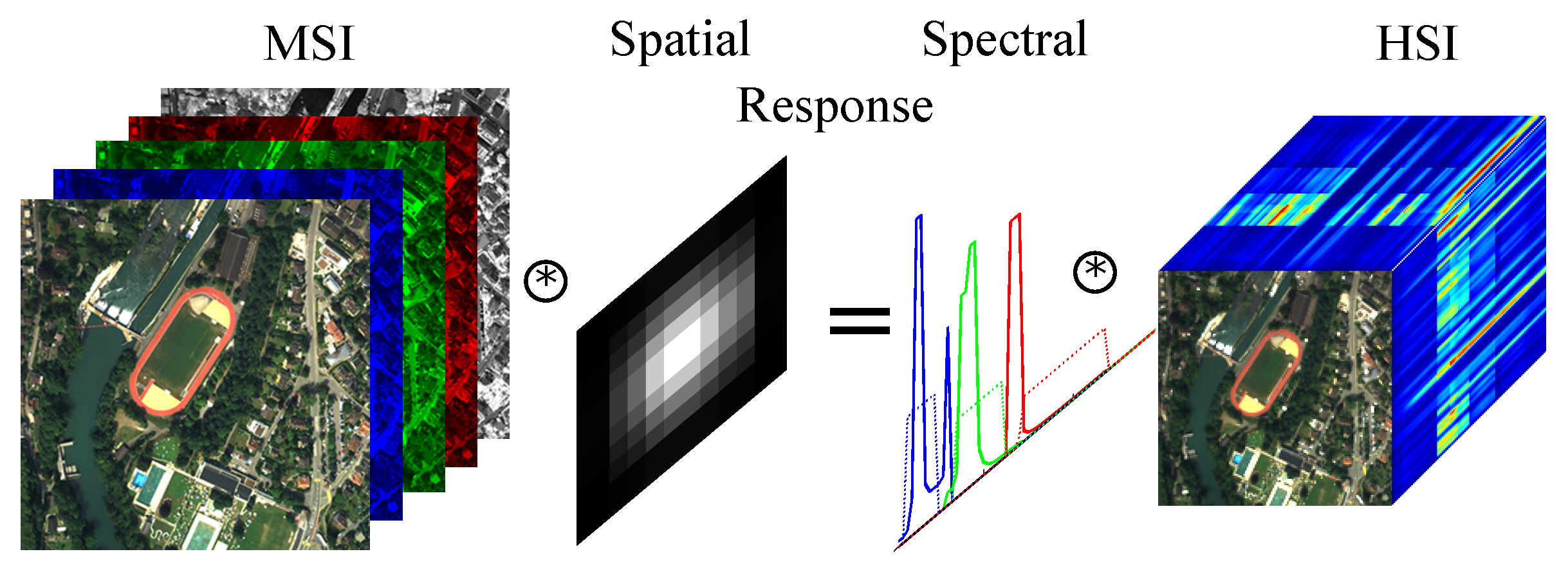
The spatial response function $\mathbf{B}$ of the hyperspectral camera and the spectral response function $\mathbf{R}$ of the multispectral sensor are either known from camera specifications, or they can be estimated directly from the data; see below. By combining Equations (2) and (3) the unknown $\mathbf{R}$ and $\mathbf{B}$ are related, up to noise, via:

$$\mathbf{M}\mathbf{B}\mathbf{S}=\mathbf{R}\mathbf{H},$$

(4)

where both sides of the equation correspond to the same image with low spectral and spatial resolution, obtained by degrading the MSI and HSI, respectively. A graphical overview of the observation model for the relative responses is shown in Figure 2.

3.1. Constraints

The core idea of the present paper is to improve super-resolution by making full use of the linear mixing model. In that model, the endmembers $\mathbf{E}$ in (1) are interpreted as reflectance spectra of individual materials, and the abundances $\mathbf{A}$ as the relative proportions of a pixel covered by those materials. As a consequence, the following physical constraints must hold:

$$\begin{array}{ll}{a}_{ij}\ge 0\forall i,j& \left(\mathrm{non-negative}\mathrm{abundance}\right)\\ {\mathbf{1}}^{\top }\mathbf{A}={\mathbf{1}}^{\top }\hfill & \left(\mathrm{abundances}\mathrm{sum}\mathrm{to}\mathrm{one}\right)\\ 0\le e_{ij}\le 1\forall i,j\hfill & (\mathrm{non-negative},\mathrm{bounded}\mathrm{reflectance})\end{array}$$

(5)

with $e_{ij}$ and $a_{ij}$ the elements of $\mathbf{E}$, respectively $\mathbf{A}$. $\mathbf{1}$ denotes a vector of one’s compatible with the dimensions of $\mathbf{A}$ and ${(·)}^{\top }$ denotes the matrix transpose. The first two constraints together bound the $l_1$-norm of the solution, and hence restrict the solution to a simplex. This means that the constraints already include the desired sparsity of the abundances (few materials, respectively endmembers per pixel). The elements of $\mathbf{E}$ have an upper bound of one, assuming that the image intensities have been rescaled to $[0\dots 1]$. That is, they behave like surface reflectances, assuming that there is at least one pure pixel in the image whose material is highly reflective in at least one spectral band.

4. Proposed Solution

4.1. Super Resolution

To solve for the super-resolved image $\mathbf{Z}$, we recover its two factors $\mathbf{E}$ and $\mathbf{A}$. From Equations (2), (3) and (5), we get the following constrained least-squares problem:

$$\begin{array}{cc}\hfill \underset{\mathbf{E},\mathbf{A}}{min}& \frac{1}{2}{\parallel \mathbf{H}-\mathbf{EABS}\parallel }_F^2+\frac{1}{2}{\parallel \mathbf{M}-\mathbf{REA}\parallel }_F^2\hfill \\ & +\frac{\lambda }{2}\parallel \mathbf{A}{\mathbf{D}}_h{\mathbf{W}\parallel }_F^2+\frac{\lambda }{2}{\parallel \mathbf{A}{\mathbf{D}}_v\mathbf{W}\parallel }_F^2\hfill \end{array}$$

(6a)

$$\begin{array}{cc}\hfill \mathrm{subject}\mathrm{to}& 0\le e_{ij}\le 1,\forall i,j\hfill \end{array}$$

(6b)

$$\begin{array}{cc}& \phantom{(}{a}_{ij}\ge 0,\forall i,j\hfill \end{array}$$

(6c)

$$\begin{array}{cc}& {\mathbf{1}}^{\top }\mathbf{A}={\mathbf{1}}^{\top }\hfill \end{array}$$

(6d)

$$\begin{array}{cc}& {\parallel \mathbf{A}\parallel }_0\le s\hfill \end{array}$$

(6e)

with ${\parallel ·\parallel }_F$ denoting the Frobenius norm and ${\parallel \mathbf{A}\parallel }_0$ the number of non-zero elements of $\mathbf{A}$. The two last (quadratic) terms of (6a) are related to the spatial information used to impose information from the MSI to the solution. ${\mathbf{D}}_h\in {\mathbb{R}}^{N_m\times N_m}$ and ${\mathbf{D}}_v\in {\mathbb{R}}^{N_m\times N_m}$ are two sparse matrices that compute the discrete gradients (differences) between neighboring pixels in horizontal, respectively vertical direction. The parameter $\lambda$ controls the strength of the regularization, and $\mathbf{W}$ is a diagonal matrix of weights that reduce the smoothness prior at high-contrast edges of the MSI, described below. The constraints in Equations (6c) and (6d) together restrict the abundances $\mathbf{A}$ to the surface of a simplex spanned by the endmembers in $\mathbf{E}$, and thus also act as a sparsity prior on the per-pixel abundances. The last constraint (6e) is optional; it serves to further increase sparsity, if desired. The diagonal values of $\mathbf{W}=diag\left(\mathbf{w}\right)$ are computed from the vector:

$$\mathbf{w}=\exp (-\frac{{(\frac{1}{Q_{95}}{\sum }_{i=1}^b{\mathbf{g}}_i)}^2}{2{\sigma }^2})$$

(7)

where $\sum {\mathbf{g}}_i$ is the sum of the (vectorized) Sobel gradient magnitudes over all b channels and $Q_{95}$ is the 95%-quantile of that vector. The latter normalizes the summed gradient magnitudes to make them invariant against the intensity range, such that the weight decay $\sigma$, which is a user-defined hyper-parameter, need not be adapted to those sensor- and scene-specific influences.

Empirically, solving Equation (6a) directly for $\mathbf{E}$ and $\mathbf{A}$ is difficult and rather unstable. The second term is strongly ill-posed w.r.t. $\mathbf{E}$ due to the spectral degradation $\mathbf{R}$, in other words only b spectral channels do not contain sufficient information to separate $p>b$ materials. Conversely, the first term is ill-posed w.r.t. $\mathbf{A}$, because the hyperspectral image, after the blurring $\mathbf{B}$ and downsampling $\mathbf{S}$, contains little information how to disentangle the abundance vector of a low-resolution pixel into contributions from its $(N_m/N_h)$ constituent high-resolution pixels. We found it advantageous to split Equation (6a) into a low-resolution ($\mathbf{H}$) and a high-resolution ($\mathbf{M}$) part and solve them by alternation. Note however, alternating between the two parts fixes their relative importance: rescaling one of the two data terms with a scalar will not affect the solution.

The low-resolution step minimizes the first term of Equation (6a) subject to the constraints on $\mathbf{E}$,

$$\begin{array}{cc}\hfill \underset{\mathbf{E}}{min}& \frac{1}{2}{\parallel \mathbf{H}-\mathbf{E}\tilde{\mathbf{A}}\parallel }_F^2\hfill \\ \hfill \mathrm{subject}\mathrm{to}& 0\le e_{ij}\le 1,\forall i,j.\hfill \end{array}$$

(8)

i.e., the endmembers of $\mathbf{H}$ are updated for given low-resolution abundances $\tilde{\mathbf{A}}$. The latter are straight-forward to obtain from (preliminary estimates of) the high-resolution abundances $\mathbf{A}$ by spatial downsampling, cf.  (2). The high-resolution step proceeds the opposite way and minimizes the second term of (6a) under the constraints on $\mathbf{A}$,

$$\begin{array}{cc}\hfill \underset{\mathbf{A}}{min}& \frac{1}{2}\parallel \mathbf{M}-\tilde{\mathbf{E}}{\mathbf{A}\parallel }_F^2+\frac{\lambda }{2}\parallel \mathbf{A}{\mathbf{D}}_h{\mathbf{W}\parallel }_F^2+\frac{\lambda }{2}{\parallel \mathbf{A}{\mathbf{D}}_v\mathbf{W}\parallel }_F^2\hfill \\ \hfill \mathrm{subject}\mathrm{to}& \phantom{(}{a}_{ij}>0,\forall i,j\hfill \\ & {\mathbf{1}}^{\top }\mathbf{A}={\mathbf{1}}^{\top }\hfill \\ & {\parallel \mathbf{A}\parallel }_0\le s\left(\mathrm{optional}\right)\hfill \end{array}$$

(9)

This time the abundances at full resolution are updated for given endmembers $\tilde{\mathbf{E}}$, which are again just spectrally downsampled version of the (preliminary) endmembers $\mathbf{E}$ from the low-resolution step.

4.1.1. Optimization Scheme

Both parts of the alternation are constrained least-squares problems. Inspired by the PALM (proximal alternating linearized minimization) algorithm [24], we propose to use a projected gradient method. For Equation (8) the following two steps are iterated for $q=1,2,\dots$ until convergence:

$$\begin{array}{c}{\mathbf{U}}^q={\mathbf{E}}^{q-1}-\frac{1}{c}({\mathbf{E}}^{q-1}\tilde{\mathbf{A}}-\mathbf{H}){\tilde{\mathbf{A}}}^{\top }\end{array}$$

(10a)

$$\begin{array}{c}{\mathbf{E}}^q={\mathrm{prox}}_{\mathbf{E}}\left({\mathbf{U}}^q\right)\end{array}$$

(10b)

with $c={\gamma }_1{\parallel \tilde{\mathbf{A}}{\tilde{\mathbf{A}}}^{\top }\parallel }_F$ a non-zero constant, and ${\mathrm{prox}}_{\mathbf{E}}$ a proximal operator that projects onto the constraints in Equation (8). What makes the algorithm attractive is that ${\mathrm{prox}}_{\mathbf{E}}$ is computationally very cheap: it amounts to truncating the entries of $\mathbf{U}$ to zero from below and to one from above.

Likewise, Equation (9) is minimized by iterating the following steps until convergence:

$$\begin{array}{c}{\mathbf{V}}^q={\mathbf{A}}^{q-1}-\frac{1}{d_1}{\tilde{\mathbf{E}}}^{\top }(\tilde{\mathbf{E}}{\mathbf{A}}^{q-1}-\mathbf{M})\\ -\frac{\lambda }{d_2}\mathbf{A}{\mathbf{D}}_h\mathbf{W}{\mathbf{W}}^{\top }{\mathbf{D}}_h^{\top }-\frac{\lambda }{d_3}\mathbf{A}{\mathbf{D}}_v\mathbf{W}{\mathbf{W}}^{\top }{\mathbf{D}}_v^{\top }\end{array}$$

(11a)

$$\begin{array}{c}{\mathbf{A}}^q={\mathrm{prox}}_{\mathbf{A}}\left({\mathbf{V}}^q\right)\end{array}$$

(11b)

with $d_1={\gamma }_2{\parallel \tilde{\mathbf{E}}{\tilde{\mathbf{E}}}^{\top }\parallel }_F$, $d_2={\gamma }_2{\parallel \mathbf{W}{\mathbf{D}}_v{\mathbf{D}}_v^{\top }{\mathbf{W}}^{\top }\parallel }_F$ and $d_3={\gamma }_2{\parallel \mathbf{W}{\mathbf{D}}_h{\mathbf{D}}_h^{\top }{\mathbf{W}}^{\top }\parallel }_F$ non-zero constants and ${\mathrm{prox}}_{\mathbf{A}}$ a proximal operator that projects onto the constraints in (9). Again, the proximal operator for the simplex projection is computationally efficient, see [25]. The complete optimization scheme is given in Algorithm 1.

Algorithm 1 Solution of minimization problem Equation (6a).

Require: $\mathbf{H},\mathbf{M},\mathbf{S},\mathbf{R}$

Initialize ${\mathbf{E}}^{\left(0\right)}$ with SISAL and ${\tilde{\mathbf{A}}}^{\left(0\right)}$ with SUnSAL

Initialize ${\mathbf{A}}^{\left(0\right)}$ by upsampling ${\tilde{\mathbf{A}}}^{\left(0\right)}$

$k\leftarrow 0$

while $notconverged$ do

$k\leftarrow k+1$

// low-resolution step:

$\phantom{(}\tilde{\mathbf{A}}\leftarrow {\mathbf{A}}^{(k-1)}\mathbf{BS}$$;$ Estimate ${\mathbf{E}}^{\left(k\right)}$ with (10a) and (10b)

// high-resolution step:

$\phantom{(}\tilde{\mathbf{E}}\leftarrow {\mathbf{RE}}^{\left(k\right)}$$;$ Estimate ${\mathbf{A}}^{\left(k\right)}$ with (11a) and (11b)

end while

return $\mathbf{Z}={\mathbf{E}}^{\left(k\right)}{\mathbf{A}}^{\left(k\right)}$

Since Equation (6a) is highly non-convex, we need good initial values to start the local optimization. We choose the SISAL algorithm [26] to initialize the endmembers in $\mathbf{E}$. SISAL robustly fits a minimum-volume simplex to the response vectors (the columns) of $\mathbf{H}$ with a sequence of augmented Lagrangian optimizations, and returns the vertices of the simplex as endmembers. With the initial endmembers ${\mathbf{E}}^{\left(0\right)}$ we then use SUnSAL [27] to get initial abundances. SUnSAL includes the constraints in Equations (6c) and (6d) and solves a constrained least-squares problem for ${\tilde{\mathbf{A}}}^{\left(0\right)}$, via alternating direction method of multipliers (ADMM). Finally, we initialize ${\mathbf{A}}^{\left(0\right)}$ by upsampling ${\tilde{\mathbf{A}}}^{\left(0\right)}$.

We always set ${\gamma }_1={\gamma }_2=1.01$. The choice of these parameters, which control the step size of the iterative minimization, affects only the computation time, not the final result. In our experience, the optimization exhibits monotonic convergence.

4.2. Relative Spatial Response

Using only image observations, one can generally not recover absolute sensor characteristics, but only the relative response of one sensor with respect to the other. The spectral and spatial response functions are coupled, since one must be known in order to directly solve for the other, as can be seen from Equation (4). In practice, we found that estimating them in two consecutive steps is sufficient. Iterating the two steps is possible, but brings no significant improvement.

Estimating the spatial response function amounts to finding the discrete 2D blur kernel that maps MSI pixels onto HSI pixels. We assume a separable kernel and split it into horizontal and vertical 1D components. The 1D kernels need not be Gaussian, but are assumed to be unimodal and symmetric. In other words, the kernel has a single peak, which need not be at the center, and descends symmetrically as one moves away from the peak. The two kernels can be different, to allow for anisotropic blur (particularly in remote sensing, there can be along-track blur and the across-track blur). We do not impose local smoothness of the kernel, since this tends to spread out the tails of the kernel function. The assumption of a separable and symmetric kernel may first seem a restriction, but it holds rather well for real imaging systems, and reduces the number of unknown coefficients, such that in practice, it stabilizes the estimation. We compute the unknowns of the blur kernel jointly for all MSI bands, which corresponds to the assumption that the blur of the MSI and HSI are band-independent.

The spatial resolution difference (ratio) between the HSI and MSI is $S=\sqrt{N_m/N_h}$. For simplicity, we restrict the discussion to integer ratios $S\in {\mathbb{N}}_{+}$, such that the discrete kernel has the same values everywhere in the image. Let ${\mathbf{R}}_0\in {\mathbb{R}}^{b\times B}$ be an initial approximation of the relative spectral response, which reduces the number of spectral channels from B to b. Using the approximate spectral response does not change the sharpness of the image [22], thus we can start by first estimating the spatial response. Let ${\mathbf{h}}_0={\mathbf{R}}_0\mathbf{H}\in {\mathbb{R}}^{b\times N_h}$ denote the image created from $\mathbf{H}$, having the spectral channels of $\mathbf{M}$. We seek to estimate the blur that will optimally fit $\mathbf{M}$ to $\mathbf{h}$ under some spatial subsampling. The search window size for the blur coefficients (in units of MSI pixels) is $W=(2k+1)S$, where $k\in \mathbb{N}$ is determined empirically. For pixels $j=1,\dots ,Z$ of $\mathbf{h}$ we extract Z 1D patches of size W from $\mathbf{M}$, either horizontally or vertically. Z is the number of all HSI pixels for which the 1D kernel of size $W/S$ falls completely inside the HSI; meaning that a small border of width k pixels in the HSI is ignored, to avoid boundary effects. We solve the following optimization separately for each of the two 1D kernels:

$$\begin{array}{cc}\hfill \underset{\mathbf{b}}{min}& {\parallel \mathbf{h}-\mathbf{L}\mathbf{b}\parallel }_F\hfill \\ \hfill \mathrm{subject}\mathrm{to}& \mathbf{G}\mathbf{b}\ge 0,\hfill \end{array}$$

(12)

where ${\mathbf{b}}_i\in {\mathbb{R}}^W$ are the unknown 1D coefficients of the blur, $\mathbf{h}\in {\mathbb{R}}^Z$ are the values of $h_0$ corresponding to the center of the patches and $\mathbf{L}\in {\mathbb{R}}^{Z\times W}$ is a matrix containing the values of $\mathbf{M}$, as Z rows of W-dimensional patches. $\mathbf{G}\in {\mathbb{R}}^{W\times W}$ is a matrix whose rows compute the differences between all pairs of adjacent values in the blur kernel ${\mathbf{b}}_i$, ordered by increasing distance from the mode (value closer to the center of gravity of the kernel minus value of the more distant neighbor). It thus forces the coefficients to decrease with increasing distance from the mode. The row for the most distant kernel coefficient has only the respective element set to one, to ensure non-negativity of ${\mathbf{b}}_i$. The ordering of rows in $\mathbf{G}$ is arbitrary, by convention we set it such that the one-values lie on the diagonal. To find the center of gravity (in horizontal and vertical direction), we first get a solution of Equation (12) with $\mathbf{G}={\mathbf{I}}_W$, where $\mathbf{I}$ is the identity matrix to enforce non-negativity. The final 2D blur for band i is given by the outer product of the vertical and horizontal kernels, $\mathbf{B}={\mathbf{b}}_{ver}{\mathbf{b}}_{hor}^{\top }$.

Equation (12) is solved as a quadratic program, using the interior point method [28]. We do not constrain the kernel coefficients to sum to 1 during the estimation (although in practice their sum always stays close to one). Instead, we normalize the final blur kernel. Note that the offset between the kernel mode and the center of the kernel window corresponds to a global (shift) misregistration between the MSI and HSI. It is estimated as part of the relative spatial response. For more technical details, the interested reader is referred to our dedicated papers [29].

4.3. Relative Spectral Response

Here the aim is to estimate the shape and size of 1D kernels that integrate HSI bands into MSI bands. Approximate knowledge of the HSI and MSI spectral responses (e.g., from the sensor manufacturer) can help initialize and guide the estimation. To increase robustness, in this case we use the $l_1$-norm for the data fitting. Given that the HSI bands are very narrow, and assuming they cover the complete spectral range of the MSI, each MSI band i can be expressed as a linear combination of HSI bands.

The estimation of the spectral response $\mathbf{R}$ is thus independent for each MSI band (each row of $\mathbf{R}$), which leads to the following optimization for the unknown spectral response ${\mathbf{r}}_i\in {\mathbb{R}}^B$ of band i:

$$\begin{array}{cc}\hfill \underset{\mathbf{r}}{min}& \parallel \mathbf{F}({\mathbf{m}}_i-{\mathbf{H}}^{\top }{\mathbf{r}}_i){\parallel }_1+{\mu }_i{\parallel \mathbf{D}{\mathbf{r}}_i\parallel }_{\alpha }\hfill \\ \hfill \mathrm{subject}\mathrm{to}& \mathbf{r}⪰0,\hfill \end{array}$$

(13)

where ${\mathbf{m}}_i\in {\mathbb{R}}^{N_h}$ is the i-th MSI band, spatially downsampled with the blur $\mathbf{B}$ (computed above) and ${\mu }_i\ge 0$ is a regularization parameter to enforce smoothness of the spectral response curve for band i, using the finite difference operator $\mathbf{D}\in {\mathbb{R}}^{B-1\times B}$ to compute the differences between elements ${\mathbf{r}}_i$ for spectrally adjacent bands. The diagonal matrix $\mathbf{F}=diag(m_{i1}^2,\dots ,m_{i{N}_h}^2)\in {\mathbb{R}}^{N_h\times N_h}$ holds individual weights for the individual pixels ${\mathbf{m}}_i$. Weights are selected such that pixels with higher intensity, and thus better SNR, in band i contribute more to the estimation of ${\mathbf{r}}_i$. Empirically, this weighting stabilizes the solution. The type of norm $\alpha$ is selected to reflect prior knowledge about ${\mathbf{r}}_i$. Steep, nearly rectangular response curves, like for instance those of the ADS80or Landsat-8 OLI [30], require piecewise constant kernels and thus $\alpha =1$. While for flatter, gradually changing response curves, like those of some amateur cameras, $\alpha =2$ is preferable. (Other choices of $\alpha$ are in principle also possible, but complicate the optimization.) We do not enforce ${\mathbf{1}}^{\top }{\mathbf{r}}_i=\mathbf{1}$, meaning that the spectral response curves need not integrate to 1. In this way, one can compensate global radiometric differences between the MSI band and the matching HSI bands.

To solve Equation (13), we again use the interior point method, starting from the approximate spectral response already used in Section 4.2. In practice, one almost always knows the approximate spectral ranges of both MSI and HSI channels; hence, one can limit the search to a smaller subset of bands $\widehat{B}<B$. The appropriate subsets $\widehat{B}$ depend on the sensors used and must be specified as part of the input data. Note that restricting the search to reasonable wavelengths only places lower and upper bounds on the response curve, its exact width need not be known. The parameters ${\mu }_i$ are set individually for each band, as discussed in Section 6.1.

5. Experiments

Before getting to the results, we introduce the five (aerial, terrestrial, and satellite) datasets used in our evaluation, explain error metrics and baselines, and summarize implementation details for SupResPALM.

5.1. Datasets

5.1.1. APEX and Pavia University

We test the super-resolution approach with synthetic HSI and MSI images derived from two well-known open remote sensing datasets, both captured with airborne sensors. The first test images is Pavia University. One spectral channel is displayed in Figure 11. The image was acquired with DLR’s ROSISsensor and has 608 × 336 pixels with a GSD of ≈1 m. There are 103 spectral bands spanning 0.4–0.9 µm. The second dataset was acquired by APEX [31], a sensor developed by a Swiss-Belgian consortium on behalf of ESA. APEX covers the spectral range 0.4–2.5 µm. The image is available as Open Science Dataset, has a GSD of about 2 m and was acquired in 2011 over Baden, Switzerland. A true color composite is shown in Figure 7. We crop an image of 400 × 400 pixels, with 211 spectral bands, after removing water absorption bands.

We follow the experimental procedure used in most of the previous work: the original hyperspectral image serves as ground truth, and the input HSI and MSI are simulated by synthetically degrading it. In all cases, we chose $\mathbf{B}$ to be Gaussian blur, with variance depending on the resolution difference S. For APEX and Pavia University, we select $S=8$ and a variance of 4 MSI pixels. For each image, we first apply the blur $\mathbf{B}$ and then subsample with the given rate S to obtain the HSI.

The MSI were created similarly, by integrating over the original spectral channels with a given spectral response $\mathbf{R}$. In the case of Pavia University, we use the spectral response of IKONOS, as also done in [11,32], since the two sensors have a fairly good spectral overlap. On the contrary APEX cover a bigger range than existing airborne mapping cameras. We use the spectral response of ADS80, which leads to a partial spectral overlap, since ADS80 does not capture wavelengths beyond 900 nm. The area under all the spectral response curves is normalized to 1 to ensure all MSI bands have the same intensity range.

5.1.2. CAVE and Harvard

To further evaluate our method, we use two publicly available hyperspectral close-range databases. The first database, called CAVE [33], includes 32 indoor images showing, e.g., paintings, toys, food, etc., captured under controlled illumination. The dimensions of the images are 512 × 512 pixels, with 31 spectral bands, each 10 nm wide, covering the visible spectrum from 400–700 nm. The second database, called Harvard [34], has 50 indoor and outdoor images recorded under daylight illumination, and 27 images under artificial or mixed illumination. The spatial resolution of these images is 1392 × 1040 pixels, with 31 spectral bands of width 10 nm, ranging from 420–720 nm. We use only the top left 1024 × 1024 pixels to avoid fractional coverage of the HSI pixels, in accordance with [10]. For CAVE and Harvard we use the extreme value of $S=32$, the standard in the existing literature. The corresponding variance of the Gaussian blur is set to 16 MSI pixels. We use the spectral response $\mathbf{R}$ of a typical digital camera, the Nikon D700 (www.maxmax.com/spectral_response.htm).

For all the above cases, we use the known spectral ($\mathbf{R}$) and spatial ($\mathbf{B}$) responses in the experiments and also assume perfect co-registration, in order to obtain a fair and meaningful comparison to the super-resolution baselines, who also assume perfectly known response functions. In the simulations, we add Gaussian noise of $\mathrm{SNR}=30\mathrm{dB}$ to the HSI and $\mathrm{SNR}=40\mathrm{dB}$ to the MSI, to simulate independent sensor noise.

5.1.3. Real EO-1 Data

Finally, we add a test case where the HSI and MSI inputs are not synthesized from the same source, but are real images as captured by a contemporary earth observation platform. The HSI and the MSI were acquired on 18 June 2016 by the Hyperion, respectively ALI sensors on board USGS’s EO-1 satellite. They show the Rhine river on the border of southern Germany and France. We crop a region of 198 × 500 pixels, with all 198 calibrated bands of Hyperion (spectral range 0.4–2.5 mm, original GSD 30 m), and the 9 multispectral bands of ALI (GSD 30 m GSD). Since, unfortunately, ALI has only limited resolution that does not exceed Hyperion, we were obliged to synthetically downsample the HSI to a GSD of 120 m also for these experiments. On the other hand, this has the advantage that we can treat the original 30 m HSI as ground truth for evaluation.

The HSI is simulated by blurring with a Gaussian of variance of 2 pixels and subsampling with stride 4, to obtain an input HSI with GSD 120 m, four times larger than the MSI. A true color composite of the scene is shown in Figure 9.

5.2. Error Metrics and Baselines

As primary error metric, we measure the root mean square error between the estimated high-resolution hyperspectral image $\widehat{\mathbf{Z}}$ and the ground truth $\mathbf{Z}$, scaled to an 8-bit intensity range $[0\dots 255]$.

$$\mathrm{RMSE}=\sqrt{\frac{1}{B{N}_m}\sum \sum {({\widehat{z}}_{ij}-z_{ij})}^2}=\sqrt{\frac{\phantom{(}\parallel \widehat{\mathbf{Z}}{-\mathbf{Z}\parallel }_F^2}{\phantom{(}B{N}_m}}$$

(14)

As a second error measure, we compute the Erreur Relative Globale Adimensionnelle de Synthèse [35], which is independent of the intensity units and also takes into account the the GSD difference between the HSI and MSI.

$$\mathrm{ERGAS}=\frac{100}{S}\sqrt{\frac{1}{B}\sum \frac{\mathrm{MSE}({\widehat{\mathbf{z}}}_i,{\mathbf{z}}_i)}{{\mu }_{\widehat{\mathbf{z}}}^2\mathit{i}}},$$

(15)

where S is the ratio of GSD difference of the MSI and HSI, $\mathrm{MSE}({\widehat{\mathbf{z}}}_i,{\mathbf{z}}_i)$ is the mean squared error of every estimated spectral band ${\widehat{\mathbf{z}}}_i$ and ${\mu }_{\widehat{\mathbf{z}}}\mathit{i}$ is the mean value of each spectral band.

Additionally, we also compute the the spectral angle mapper (SAM [36]), which is defined as the angle in ${\mathbb{R}}^B$ between the estimated spectrum ${\widehat{\mathbf{z}}}_j$ and the ground truth spectrum ${\mathbf{z}}_j$, averaged over all pixels.

$$\mathrm{SAM}=\frac{1}{N_m}\sum arccos\frac{{\widehat{\mathbf{z}}}_j^{\top }{\mathbf{z}}_j}{\parallel {\widehat{\mathbf{z}}}_j{\parallel }_2{\parallel {\mathbf{z}}_j\parallel }_2}$$

(16)

where ${\parallel ·\parallel }_2$ is the $l_2$ vector norm. The SAM is given in degrees, and compares only the shape of the predicted spectra, while ignoring differences in magnitude (scale of the response vector). As a final quality metric we use $\mathrm{Q}{2}^n$, an extension of the Universal Image Quality Index (UQI) from single-band to multispectral/hyperspectral images, based on hypercomplex numbers [37]. The $\mathrm{Q}{2}^n$ takes on values between $-1$ (worst) and 1 (best).

As baselines to compare against, we use four state-of-the-art methods, which we term: CNMF [12], SNNMF [13], HySure [11] and R-FUSE [18]. These baselines were chosen because for them the best results are reported in the literature, and the source code for all of them was made available by the authors. We thus run the authors’ original implementations and tune them for best performance on the datasets used in our study. Furthermore, we report the error metrics for the naively magnified HSI (using bicubic interpolation), as a baseline for upsampling without the additional information from the MSI.

5.3. Implementation Details

The inner loops of the two optimization steps (10a) and (11a) are run until the update falls below 1%, which typically takes ≈10 iterations in the early stages and drops to ≈2 iterations as the alternation proceeds. The outer loop over the two steps is iterated until the overall cost (6a) changes less than 0.01%, or for at most 2000 iterations. In simulated data the limit of 2000 is reached in several cases, while with real data the algorithm converges in a few tens of iterations. As a default setting for our method we use smoothing with $\lambda =0.1$, except if stated otherwise. The parameter that governs the contrast-sensitivity of the smoothing is set to $\sigma =1.5$. Perhaps the most important user parameter is the number p of endmembers. This parameter depends on the scene contents and according to our experience $p=30$ is sufficient for most Remote Sensing images. In the case of CAVE and Harvard datasets, with much fewer bands and fewer materials per image we reduce p to 10. We use the same number of basis vectors in all baselines. The final results may vary slightly, due to random sampling in the VCA initialization (for SupResPALM and also for HySure and CNMF). Our current implementation in MATLAB 9.0 has not been optimized for speed. Computation times depend on the image size and the number of iterations, as well as the sparsity parameter s, if used. For the EO-1 data with dimensions 500 × 180 pixels and 198 channels it takes ≈1 min, on a single Intel Xeon E5 3.2 GHz CPU.

6. Experimental Results and Discussion

We now present and discuss the empirical performance of the proposed super-resolution scheme. To keep the length of the paper reasonable, not all available results are presented, since many experiments exhibit similar trends and support the same conclusions. Complementary tables and figures are available in the Supplementary Materials.

6.1. Relative Responses

6.1.1. CAVE Database

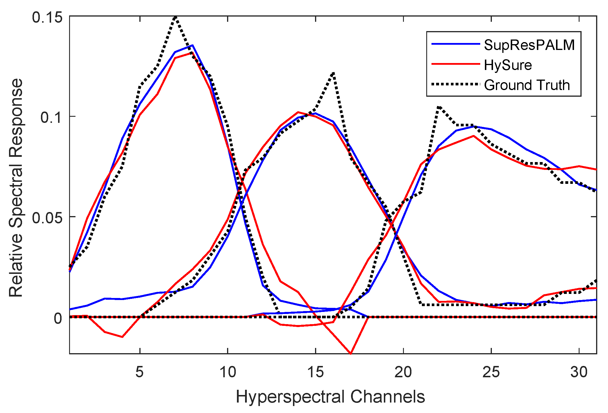
As baseline for this evaluation we only use HySure, because it is the only one among our baselines that can recover the relative responses from the data. To evaluate the estimation of the spectral response test on a simulated MSI from the CAVE database and compare to the actually used response function (cf. Section 5.1.2). The results are shown in Figure 3. The estimated response curves are in both cases fairly close to the true ones (dashed line). However, HySure returns a number of negative response values, which SupResPALM avoids by construction. The latter was run with the setting for smooth responses, $\alpha =2$. Regarding the spatial response function, please refer to the following section.

6.1.2. Real EO-1 Data

For the EO-1 data we estimate the relative responses from the data as described in Section 4.2 and Section 4.3. Since the low resolution HSI was simulated with a known blur kernel, we can evaluate the results of both SupResPALM and HySure against the ground truth, see Figure 4a. The estimated spatial responses can be seen in Figure 4b for SupResPALM and Figure 4c for HySure. The full blur of SupResPALM is given as the outer product of its respective horizontal and vertical components. For the size we used a radius parameter of $k=2$, larger values give almost identical results. The spatial responses are computed over all nine spectral channels of ALI, assuming uniform blur in all channels. While HySure strongly regularizes the response functions, this tends to enlarge their spatial extents and even lead to negative values in the presence of noise. On the other hand, our method is less flexible regarding the shape of the blur, but still ensures a monotonously descending kernel, without negative values. From the estimation of the spatial response, we get a translation of $[0.07,0.11]$ MSI pixels between the two images, meaning that the two sources are coregistered very well. Still, we do account for the small shift during fusion, by using the estimated, slightly decentered blur kernel.

The spectral response is then estimated at low spatial resolution, i.e., from our input HSI and a degraded MSI with 120 m GSD, downsampled with the estimated blur (Figure 4). For comparison, we also ran the estimation of the spectral response at high resolution, using “ground truth” HSI and the input MSI with 30 m GSD. This control experiment excludes any possible influence of the (estimated) spatial blur, but gives practically identical results.

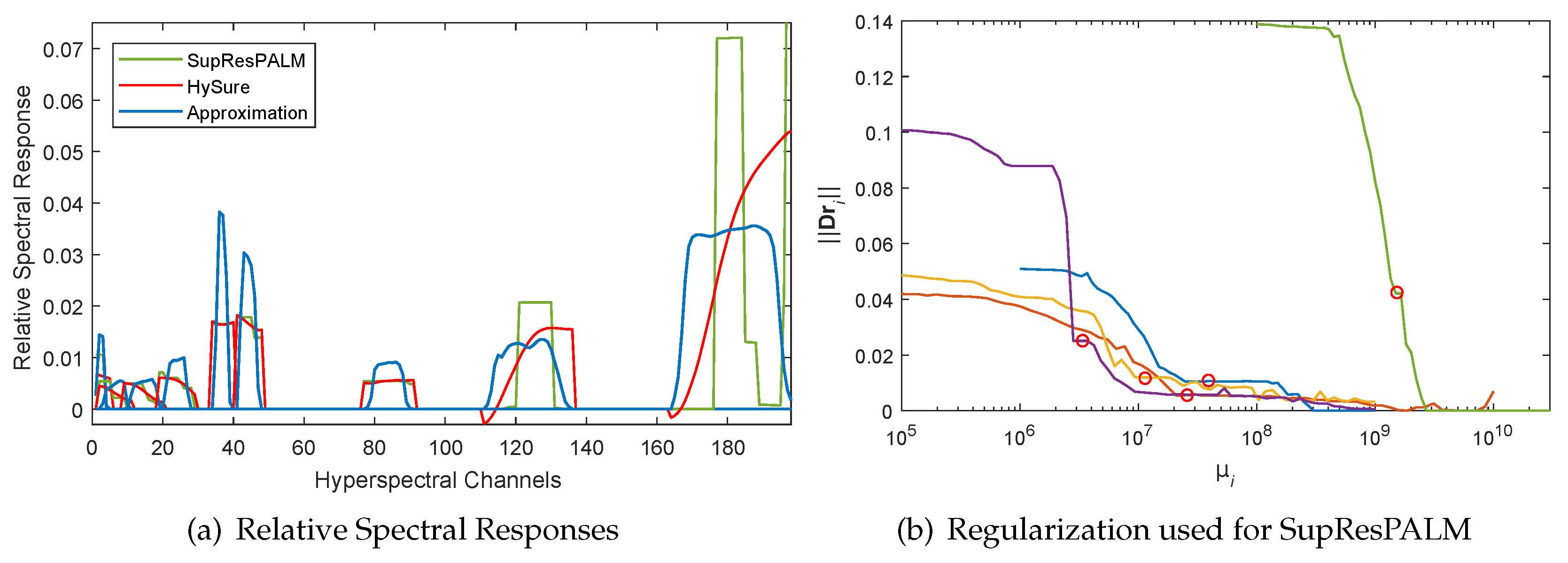
The results of both methods are shown in Figure 5a. Unfortunately, there is no ground truth for the spectral responses. We do have approximate values computed from the specified absolute responses of the two sensors, but these do not appear to accurately represent the actual band-pass filters used. Due to the strong $l_2$ regularization, the response curves from HySure end to have non-zero values everywhere inside the maximum spectral range $\widehat{B}$ for any given channel, in some cases including implausible negative values near the spectral bounds. Our method, tuned for steep band-pass filters with $\alpha =1$, leads to more plausible results and seems to better pick up which hyperspectral bands really contribute to each MSI band, especially for longer wavelengths, see Figure 5a. Note, when run with a one-normalized spatial blur kernel, SupResPALM and HySure include the band-specific radiometric scaling in the spectral response function. The approximate values from the specifications (blue line) were re-normalized per band to have the same area under the curve as SupResPALM (respectively, HySure, the estimated areas are practically identical).

In Figure 5b, we plot the influence of the regularization term $\parallel \mathbf{D}{\mathbf{r}}_i\parallel$ against its weight ${\mu }_i$, for five MSI (ALI) channels. The curves show a typical behavior, which we use to determine the weight: for too low values the band-to-band differences remain constant (no smoothing), for too high values they vanish (strong oversmoothing). In between there typically is a region where the curves flatten out to return similar results across a range of weights (denoted with red circles). We found that choosing weights from those intermediate plateaus, where the solution is rather stable, yields good spectral responses. In general the spectral responses remain reasonable over a wide range of values, and their exact shape has only a small effect on the final super-resolution. Even simple heuristics like using half of the maximum (unsmoothed) $\parallel \mathbf{D}{\mathbf{r}}_i\parallel$ will give very reasonable results, see Section 6.2.3.

6.2. Super-Resolution

6.2.1. APEX and Pavia University

The numerical results for the two aerial datasets are displayed in

Table 1. Quantitative results for APEXand Pavia University. SAM, spectral angle mapper.

Method	APEX				Pavia University
	RMSE	ERGAS	SAM	Q2n	RMSE	ERGAS	SAM	Q2n
SNNMF	8.82	3.23	8.53	0.812	2.76	0.97	3.10	0.918
HySure	8.75	3.15	7.44	0.756	2.33	0.83	2.76	0.928
R-FUSE	9.29	3.53	7.70	0.757	3.36	1.22	3.50	0.854
CNMF	9.17	3.35	7.41	0.757	2.33	0.85	2.48	0.892
SupResPALM	8.23	3.02	7.27	0.821	2.28	0.79	2.41	0.935

(best results in bold). SupResPALM achieves lower errors than all four baselines, in all metrics. The difference is more pronounced in the case of APEX, which is the harder dataset, due to the only partial spectral overlap between HSI and MSI. The effect becomes evident in Figure 6, where the RMSE per band is plotted for both images. For APEX (left) there is a sudden increase in the RMSE value around band 100, where the spectral sensitivity of the ADS80 ends. Of course, also our method has higher errors in this extrapolated part of the spectrum, still it achieves lower errors than the baselines. For Pavia University, the RMSE values are fairly constant throughout the spectrum, except near the two ends of the spectral coverage, in which wavelengths the channels are noisier.

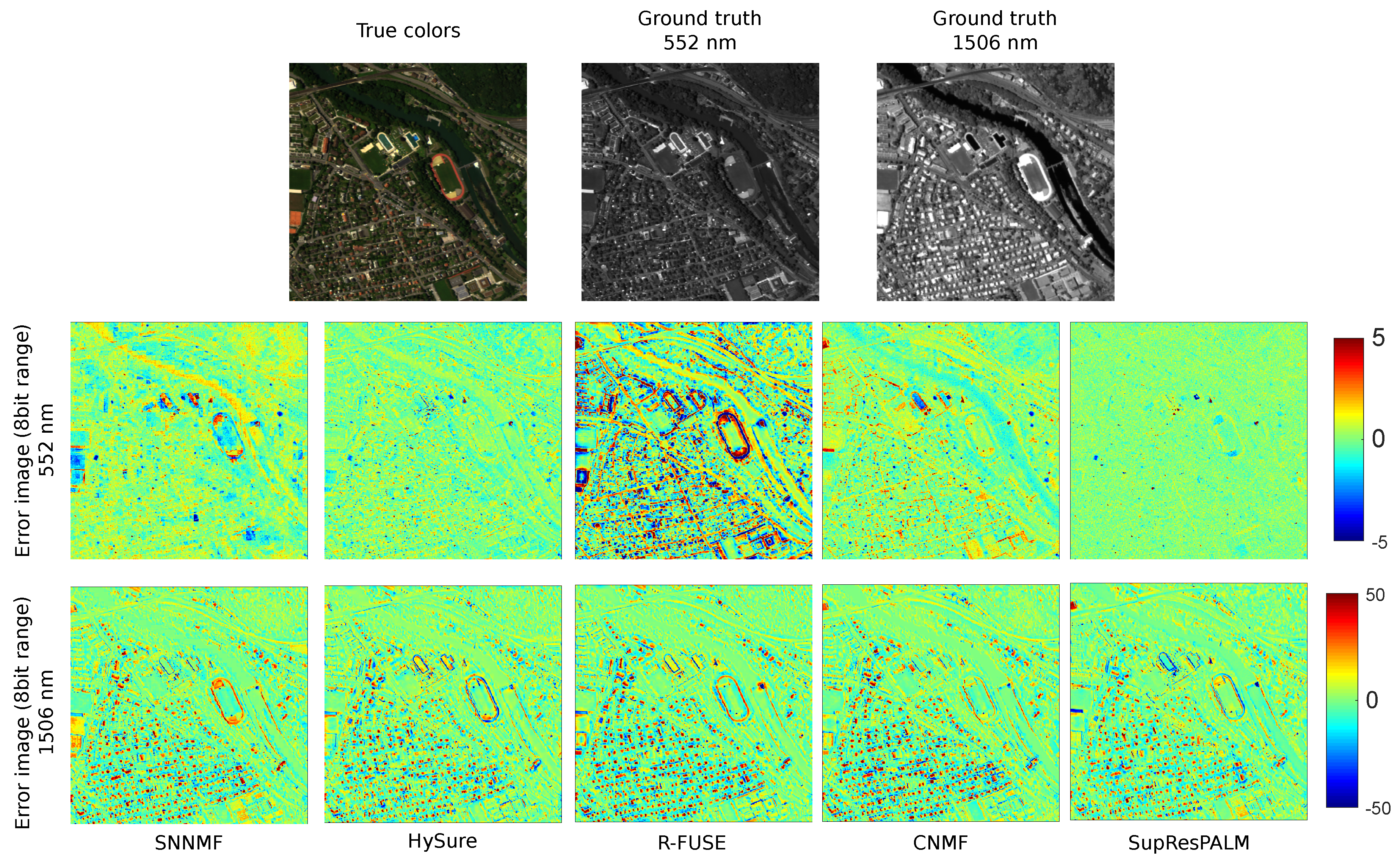
Moreover, we visualize the errors of all methods, in two different bands. We do this for APEX, since it is the more challenging scene, reconstruction errors are bigger, and the scene has a larger variety of distinguishable surface materials. In Figure 7 we plot the errors, in 8-bit range, for wavelengths 552 and 1506 nm. The first wavelength corresponds to a low reconstruction error (overlap with MSI), while the second one lies outside the MSI range and has high reconstruction error.

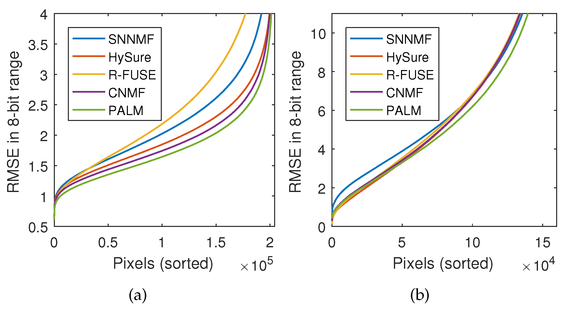
Moreover, we plot the cumulative histogram of per-pixel residuals. In Figure 8 all pixels of a scene are sorted by their RMSE (norm of residual vector across all channels), in ascending order. Horizontal cuts correspond to the number of pixels below a fixed RMSE tolerance, vertical cuts correspond to the minimum error one must accept when using only a fixed number of “best” pixels. From these graphs it can be seen that our method has the largest amount of pixels with the low reconstruction errors. Note the different scaling of the axes; the gains are actually greater for APEX than for Pavia.

6.2.2. CAVE and Harvard

For CAVE and Harvard we focus on the numerical results. Please refer to [5] for visualizations.

Table 2. Quantitative results for the CAVEDatabase.

Method	CAVE Database
	RMSE			ERGAS			SAM			Q2n
	Aver.	Med.	1st	Aver.	Med.	1st	Aver.	Med.	1st	Aver.	Med.	1st
Bic. upsampling	24.14	22.03	0	3.191	3.157	0	16.01	15.83	0	0.810	0.837	0
SNNMF	4.47	4.29	0	0.590	0.570	0	18.13	19.60	0	0.909	0.935	2
HySure	4.50	3.94	0	0.563	0.536	1	19.27	19.05	0	0.913	0.938	4
R-FUSE	4.16	3.74	1	0.644	0.526	1	8.61	8.28	2	0.912	0.933	5
CNMF	3.54	2.92	8	0.490	0.420	8	7.16	7.05	7	0.913	0.940	2
SupResPALM	3.15	2.88	23	0.430	0.351	22	6.46	6.54	23	0.927	0.948	19

and

Table 3. Quantitative results for the Harvard database.

Method	Harvard Database
	RMSE			ERGAS			SAM			Q2n
	Aver.	Med.	1st	Aver.	Med.	1st	Aver.	Med.	1st	Aver.	Med.	1st
Bic. upsampling	12.97	12.30	0	1.481	1.437	0	5.50	5.22	0	0.863	0.921	0
SNNMF	2.47	2.04	2	0.411	0.354	2	5.25	4.47	0	0.925	0.965	11
HySure	2.18	1.86	0	0.390	0.335	1	4.75	4.10	1	0.929	0.966	7
R-FUSE	2.28	2.01	0	0.398	0.372	0	3.87	3.71	1	0.927	0.960	3
CNMF	1.91	1.61	20	0.299	0.286	24	3.15	2.99	36	0.926	0.964	7
SupResPALM	1.81	1.53	55	0.318	0.278	50	3.16	3.04	39	0.934	0.969	49

show the error metrics (best results in bold) that each method achieved in both full datasets. We only report average and median RMSE, ERGAS, SAM and $\mathrm{Q}{2}^n$ values, as well as the number of images that each method reconstructed best. Complete per-image numbers are available in the Supplementary Materials. Again SupResPALM outperforms all baselines in a clear majority of images. The errors and differences are greater on CAVE for all methods, which has a larger number and variability of materials per image. We also report for how many images each method returned the best result, in each error metric. That number gives an intuition whether a method is consistently better than another one across different images.

6.2.3. Real EO-1 Data

The main challenge of this dataset, compared to the simulated data, is that the input images originate from two different sensors with individually different, non-Gaussian noise. Moreover, like in the APEX scene, the spectral ranges of the HSI and the MSI do not fully overlap. The numerical results of the super-resolution are given in

Table 4. Quantitative results of SupResPALM for Real EO-1 data.

EO-1 Real Data
Method	RMSE	ERGAS	SAM	Q2n
Bicubic upsampling	5.99	12.58	4.06	0.547
SupResPALM $\lambda$ = 0, $s=5N_m$	3.63	13.49	3.01	0.765
SupResPALM $\lambda$ = 0.01, $s=5N_m$	3.61	13.52	3.10	0.764
SupResPALM $\lambda$ = 0	3.48	13.50	2.85	0.774
SupResPALM $\lambda$ = 0.01	3.39	13.58	2.80	0.776

. We test SupResPALM in four configurations, where we compare different values for the sparsity of the endmembers and the spatial regularization. Empirically, the spatial regularization has only a small influence, whereas limiting the average number of active endmembers per pixel with the sparsity constraint, Equation (6e), produces a noticeable increase in reconstruction error. In this previous experiment the reconstruction is done with relative response functions estimated from the data with SupResPALM. We further test the SupResPALM super-resolution with HySure responses and vice versa, to separate the estimation of the response functions from the super-resolution itself,

Table 5. Comparison of SupResPALM and HySure on real EO-1 data, separating estimation of response functions and super-resolution. Best results with bold, second best in Italics.

		Relative Responses
		HySure	SupResPALM
R-FUSE	RMSE	3.89	3.91
	ERGAS	13.81	13.80
	SAM	3.40	3.52
	Q2n	0.747	0.752
HySure	RMSE	4.77	4.76
	ERGAS	14.18	14.19
	SAM	3.97	3.97
	Q2n	0.698	0.698
SupResPALM $\lambda =0.01$	RMSE	3.34	3.39
	ERGAS	13.73	13.58
	SAM	2.75	2.80
	Q2n	0.775	0.776

. Not all baselines allow one to input the relative responses. SNNMF has memory issues and cannot handle the estimated spatial response function, whereas CNMF assumes a fixed spatial response and lets the user chose only the spectral response. In R-FUSE it is possible to input both response functions, so we include it in Table 5. It turns out that small variations in the relative sensor characteristics do not have a significant impact on the super-resolution. While SupResPALM super-resolution, with different reasonable response functions, outperforms HySure and R-FUSE by a clear margin.

The reconstructed Hyperion images of both methods, as well as the ground truth, are shown as color composite in Figure 9. SupResPALM produces visibly fewer and weaker artifacts than HySure and R-FUSE. Nevertheless, some areas do exhibit spectral distortions, e.g., the small lake above the river in the middle of the image. These qualitative and quantitative results are, in our view, a much stronger indication than purely synthetic experiments that SupResPALM can be applied to real data.

6.3. Discussion

6.3.1. Spectral Unmixing

Introducing the spectral unmixing constraints has proven to give good numerical results and plausible mixtures of materials. In Figure 10 are the abundances of selected endmembers, which correspond to easily recognizable surface materials observed in the APEX scene. Even though these are not always “pure materials” in the physical sense, due to non-linearities like inter-reflections, specularities and shadows, they look realistic, and comparatively clean. This confirms the conventional wisdom that the LMM is sufficient for many hyperspectral imaging problems, including in particular super-resolution. We also note that enforcing non-negativity of the solution and the sum-to-one constraint has very pragmatic advantages for further processing. Without the explicit constraints, artifacts do occur, like negative reflectance values, or pixels with reflectance zero in all bands. These mistakes may disturb further processing. As a simple example, for the spectral power zero the computation of the SAM will fail (for our baselines, we have excluded such pixels from the error computation).

SupResPALM has one main user parameter, namely p, the number of the endmembers (the subspace dimension). Note that classic dimensionality estimation methods do not apply in our case, where both the basis and the coefficients are constrained. If the main goal is super-resolution (and not accurate and unambiguous unmixing), one can in our experience use the upper bounds $p=30$ for remote sensing scenes with hundreds of bands, and $p=10$ for close-range scenes with ≈30 bands.

6.3.2. Effect of the Sparsity Term

As discussed in Section 4, our framework allows one to explicitly limit the average number of active endmembers per pixel, via Equation (6e). Although the simplex constraint favors sparse solutions, sometimes it may be desired to enforce stronger sparsity, by suppressing small abundance values. Sparser solutions will typically yield more realistic endmembers and abundances, by eliminating “garbage collection” endmembers that fit systematic effects like shading variations. However, in general, they will produce worse reconstruction results, because eliminating systematic errors obviously benefits the super-resolution, even if done by “misusing” the linear mixing model. For instance, a single, complex material can exhibit spectral shifts due to shading effects and give rise to two slightly different endmembers. Eliminating one of them improves the correspondence between endmembers and materials, but increases the super-resolution error. In

Table 6. Effect of the sparsity parameter s for APEX and Pavia University. The first row is the selected sparsity level (average number of non-zero endmembers per pixel). The values in the first column are without the additional sparsity term.

	APEX						Pavia University
s/Nm	–	6	5	4	3	2	–	6	5	4	3	2
RMSE	8.23	8.29	8.46	8.68	9.07	10.31	2.28	2.61	2.79	3.18	4.29	7.87
ERGAS	3.02	3.06	3.14	3.24	3.42	4.01	0.79	0.93	0.98	1.09	1.36	2.26
SAM	7.27	6.96	7.02	7.18	7.57	9.17	2.41	2.72	2.88	3.22	4.00	6.08
Q2n	0.821	0.811	0.810	0.808	0.790	0.696	0.935	0.925	0.914	0.883	0.793	0.664

we show a quantitative evaluation on APEX and Pavia University for different $s/N_m$ ratios ranging from 2–6. Both images initially have ≈20 average active endmembers per-pixel with basic SupResPALM. As we push down that number, the accuracy slowly drops, as expected. While the drop for Pavia University becomes rather severe, APEX can be super-resolved acceptably well with only $3N_m$ non-zero abundances (RMSE still lower than several baselines). We attribute this behavior to the scene content of Pavia University, where many small objects exist that cause mixed pixels.

The extra sparsity is also applied to the CAVE database (

Table 7. Effect of the sparsity parameter s for CAVE. The first row is the selected sparsity level (average number of non-zero endmembers per pixel). The values in the first column are without the additional sparsity term.

	CAVE Database
s/Nm	–	6	5	4	3	2
RMSE	3.15	3.18	3.23	3.32	3.77	5.18
ERGAS	0.430	0.436	0.443	0.457	0.531	0.700
SAM	6.46	6.41	6.56	6.75	7.46	8.56
Q2n	0.927	0.927	0.926	0.923	0.920	0.904

) with the $s/N_m$ ratio between six and two. Since the CAVE images are taken from close range and have a limited number of mixed pixels, restricting $s=3N_m$ still gives a better reconstruction than most baselines, while maintaining a plausible explanation about the scene’s endmembers and abundances. A similar effect is observed for the Harvard database. For details, see the Supplementary Materials. Again, increased sparsity through a stricter s appears to reduce over-fitting of the unmixing and lead to physically more plausible endmembers by suppressing overly small abundances. However, as shown in Table 4, Table 6 and Table 7, this will usually not improve the super-resolution.

6.3.3. Effect of the Spatial Regularization

We have also tested the spectral unmixing approach without the spatial regularization on APEX and Pavia University images (

Table 8. Effect of the spatial regularization on APEX and Pavia.

Method SupResPALM	APEX				Pavia University
	RMSE	ERGAS	SAM	Q2n	RMSE	ERGAS	SAM	Q2n
$\lambda =0.1$	8.23	3.02	7.27	0.821	2.28	0.791	2.41	0.935
$\lambda =0$	8.19	2.98	6.98	0.822	2.34	0.817	2.42	0.935

). We conjecture that spatial smoothing may in fact not be all that important, if the super-resolution is sufficiently constrained by other means. In particular, we found that the simplex constraint (6c) and (6d), that abundances must be non-negative and sum to 1 very effectively stabilizes the prediction, such that further regularization may not be necessary; while they have not been used in this form before. As it happens, our method performs almost equally well with $\lambda =0$ (no spatial regularization). There are differences, but they are very small, and not always in favor of spatial smoothing, see Table 8. However, in the EO-1 experiment the spatial regularization does improve the super-resolution, see Table 4. We believe this is due to the fact that a realistic (slightly spatially variant) misalignment is present between the EO-1 images that where actually acquired by distinct sensors, the effect of which can be mitigated by moderate smoothing. While further work is needed to clarify the role of smoothing, at this point we recommend to retain it for real applications with separate MSI and HSI sensors.

6.3.4. Denoising

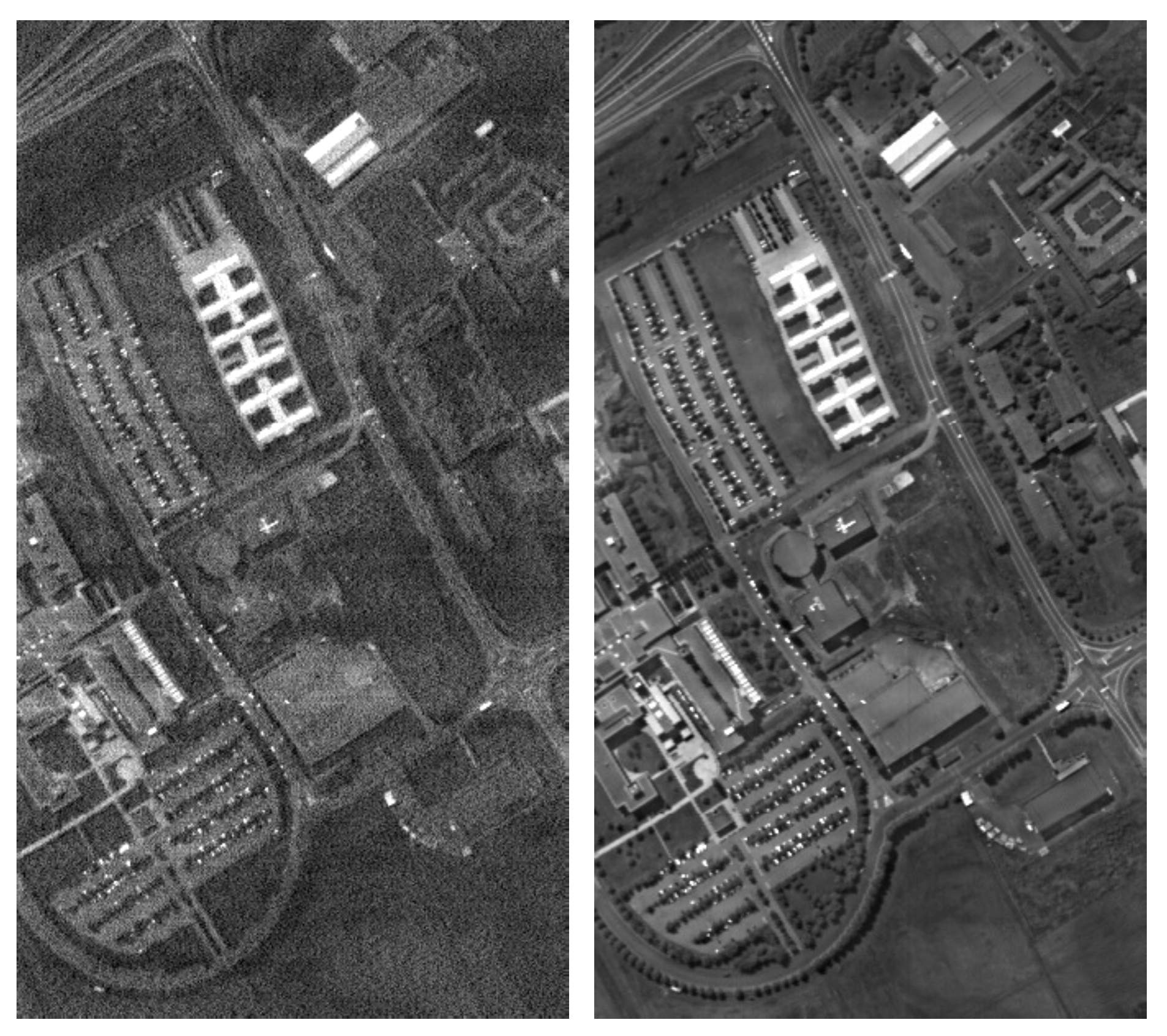
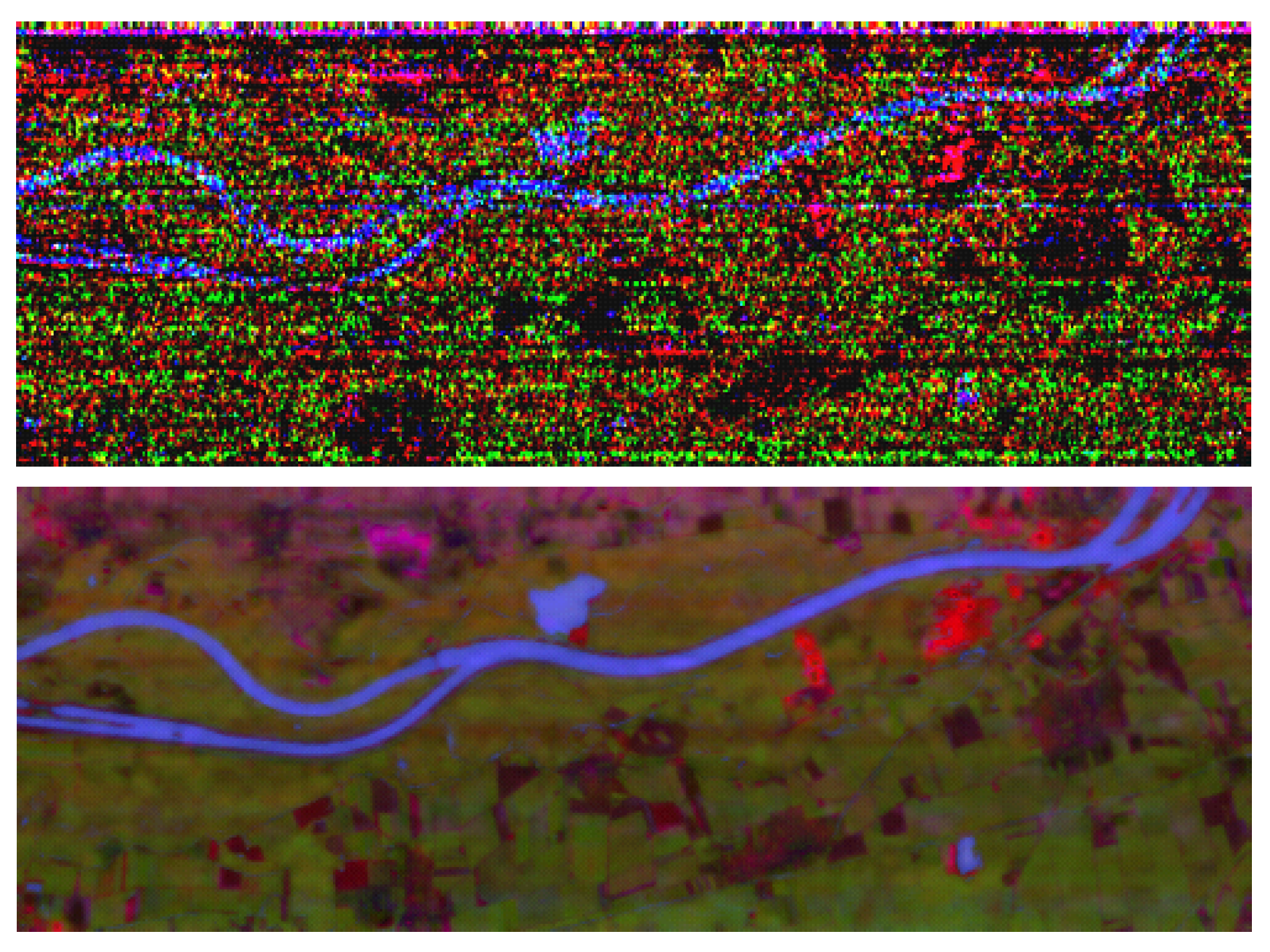
Hyperspectral images are often quite noisy, mainly due to sensor limitations and atmospheric effects. Figure 11 shows the first band (≈400 nm) of the Pavia University image. On the left is the original, noisy “ground truth” image, on the right the super-resolution reconstruction by SupResPALM. Obviously, much of the noise has been removed, because the high-frequency content of the reconstruction is obtained from the MSI, which is less corrupted as the spectral integration cancels noise (no matter whether it is done in software or by wider band-pass filters). We point out that this rather beneficial effect does not show up in the quantitative results: on the contrary, it increases the deviation from the noisy ground truth (for all methods). The effect is even stronger for Hyperion (EO-1), where many of the short-wave infrared bands have very low power and are very noisy, see Figure 12. At the top is an amplified color composite of bands 125, 173 and 181 of the high resolution HSI, below is our reconstruction. The fusion has produced a much clearer image, with clear and homogeneous geographic features that are barely observable in the original. Similar results have also been reported by Cerra et al. [38] in the context of hyperspectral image denoising.

7. Conclusions

We have proposed a method for hyperspectral super-resolution. Its basic idea is to jointly solve the spectral unmixing problem for both input images. Linking super-resolution to unmixing allows one to constrain the solution to conform with the elementary physics of optical imaging. We argue that this might be a more suitable way to regularize the inherently ill-posed super-resolution task. Given a spatially-coarse hyperspectral image and a spectrally-coarse, high-resolution MSI image, we estimate an image with high spatial and spectral resolution. As a side effect, our method additionally delivers a set of spectral endmembers and physically-plausible decomposition of each pixel into those endmembers. Under the linear mixing model, the proposed approach boils down to two coupled, constrained least-squares problems, which can be solved reliably with a projected gradient scheme. We found that updating also the basis, rather than only the mixing coefficients, during super-resolution gives better results, and recommend it over the sequential processing of many existing methods. Additionally, we have experimented with a spatial smoothness term driven by the gradients of the high-resolution MSI. Spatial regularization is typically the first and most obvious strategy used to regularize ill-posed image processing problems. However, we found that, while it is straight-forward to include in our method, it only marginally improves the result. We thus do not generally recommend it; it seems that if one has access to other, less “diffuse” a priori knowledge like our unmixing constraints, explicit spatial smoothness may not be as important. Finally, we have expanded our method to work with real data, where the spatial and spectral response functions are not perfectly known, by estimating them from the images themselves. Again, we prefer to restrict the inference to plausible solutions, in this case symmetric, unimodal responses, but avoid arbitrary priors chosen for convenience (such as Gaussian responses). In simulations on four public datasets, the proposed SupResPALM method has shown excellent performance. Moreover, we have applied our method to real remote sensing data from two different satellite sensors (Hyperion and ALI), where it also worked well. While the EO-1 satellite carrying Hyperion and ALI has recently been decommissioned, a number of missions are underway that will bring new hyperspectral sensors to space in the next few years (e.g., EnMAP, PRISMA, HISUI). These missions will also benefit from improved data fusion and super-resolution. A worthwhile extension of the presented method will be to deal with cases where the HSI and MSI have not been acquired from the same platform. In that situation, additional problems arise, such as precise co-registration, handling differing viewing angles and handling temporal changes between different acquisition times.

A limitation of the current method is that linear mixing does not adequately capture the actual behavior of some important materials, in particular high vegetation including for example forest and many agricultural crops. In the current framework, non-linear BRDF effects like shading, specular reflection, cast shadows and direction-dependent reflectance are phenomenologically dissipated with additional “virtual” endmembers. For highly non-linear materials or when correct unmixing matters, one may have to extend the model to explicitly include more complex shading behavior. Furthermore, it is known that the spatial response of many sensors depends on the wavelength and sometimes also on the location in the field of view, whereas we assume a spatially isotropic and band-independent blur. Again, this does not seem to negatively affect super-resolution; still, it may be desirable to recover more detailed sensor characteristics, especially when using them in the further analysis of the data.

References

- Varshney, P.K.; Arora, M.K. Advanced Image Processing Techniques for Remotely Sensed Hyperspectral Data; Springer: Berlin, Germany, 2004. [Google Scholar]
- Yokoya, N.; Grohnfeldt, C.; Chanussot, J. Hyperspectral and Multispectral Data Fusion: A comparative review of the recent literature. IEEE Geosci. Remote Sens. Mag. 2017, 5, 29–56. [Google Scholar] [CrossRef]
- Keshava, N.; Mustard, J.F. Spectral unmixing. IEEE Signal Process. Mag. 2002, 19, 44–57. [Google Scholar] [CrossRef]
- Wang, T.; Yan, G.; Ren, H.; Mu, X. Improved methods for spectral calibration of on-orbit imaging spectrometers. IEEE Trans. Geosci. Remote Sens. 2010, 48, 3924–3931. [Google Scholar] [CrossRef]
- Lanaras, C.; Baltsavias, E.; Schindler, K. Hyperspectral Super-Resolution by Coupled Spectral Unmixing. In Proceedings of the IEEE International Conference on Computer Vision (ICCV), Santiago, Chile, 11–18 December 2015; pp. 3586–3594. [Google Scholar]
- Wang, Z.; Ziou, D.; Armenakis, C.; Li, D.; Li, Q. A comparative analysis of image fusion methods. IEEE Trans. Geosci. Remote Sens. 2005, 43, 1391–1402. [Google Scholar] [CrossRef]
- Loncan, L.; de Almeida, L.B.; Bioucas-Dias, J.M.; Briottet, X.; Chanussot, J.; Dobigeon, N.; Fabre, S.; Liao, W.; Licciardi, G.A.; Simoes, M.; et al. Hyperspectral Pansharpening: A Review. IEEE Geosci. Remote Sens. Mag. 2015, 3, 27–46. [Google Scholar] [CrossRef] [Green Version]
- Kawakami, R.; Wright, J.; Tai, Y.W.; Matsushita, Y.; Ben-Ezra, M.; Ikeuchi, K. High-resolution hyperspectral imaging via matrix factorization. In Proceedings of the IEEE Computer Vision and Pattern Recognition (CVPR), Colorado Springs, CO, USA, 20–25 June 2011; pp. 2329–2336. [Google Scholar]
- Huang, B.; Song, H.; Cui, H.; Peng, J.; Xu, Z. Spatial and spectral image fusion using sparse matrix factorization. IEEE Trans. Geosci. Remote Sens. 2014, 52, 1693–1704. [Google Scholar] [CrossRef]
- Akhtar, N.; Shafait, F.; Mian, A. Sparse Spatio-spectral Representation for Hyperspectral Image Super-Resolution. In Proceedings of the European Conference on Computer Vision, Zurich, Switzerland, 6–12 September 2014; pp. 63–78. [Google Scholar]
- Simoes, M.; Bioucas-Dias, J.; Almeida, L.; Chanussot, J. A Convex Formulation for Hyperspectral Image Superresolution via Subspace-Based Regularization. IEEE Trans. Geosci. Remote Sens. 2015, 53, 3373–3388. [Google Scholar] [CrossRef]
- Yokoya, N.; Yairi, T.; Iwasaki, A. Coupled nonnegative matrix factorization unmixing for hyperspectral and multispectral data fusion. IEEE Trans. Geosci. Remote Sens. 2012, 50, 528–537. [Google Scholar] [CrossRef]
- Wycoff, E.; Chan, T.H.; Jia, K.; Ma, W.K.; Ma, Y. A non-negative sparse promoting algorithm for high resolution hyperspectral imaging. In Proceedings of the IEEE International Conference on Acoustics, Speech and Signal Processing (ICASSP), Vancouver, BC, Canada, 26–31 May 2013; pp. 1409–1413. [Google Scholar]
- Veganzones, M.A.; Simoes, M.; Licciardi, G.; Yokoya, N.; Bioucas-Dias, J.M.; Chanussot, J. Hyperspectral super-resolution of locally low rank images from complementary multisource data. IEEE Trans. Image Process. 2016, 25, 274–288. [Google Scholar] [CrossRef] [PubMed]
- Hardie, R.C.; Eismann, M.T.; Wilson, G.L. MAP estimation for hyperspectral image resolution enhancement using an auxiliary sensor. IEEE Trans. Image Process. 2004, 13, 1174–1184. [Google Scholar] [CrossRef] [PubMed]
- Wei, Q.; Dobigeon, N.; Tourneret, J.Y. Bayesian fusion of multi-band images. IEEE J. Sel. Top. Signal Process. 2015, 9, 1117–1127. [Google Scholar] [CrossRef]
- Wei, Q.; Dobigeon, N.; Tourneret, J.Y. Fast fusion of multi-band images based on solving a Sylvester equation. IEEE Trans. Image Process. 2015, 24, 4109–4121. [Google Scholar] [CrossRef] [PubMed]
- Wei, Q.; Dobigeon, N.; Tourneret, J.Y.; Bioucas-Dias, J.; Godsill, S. R-FUSE: Robust Fast Fusion of Multiband Images Based on Solving a Sylvester Equation. IEEE Signal Process. Lett. 2016, 23, 1632–1636. [Google Scholar] [CrossRef]
- Zou, C.; Xia, Y. Hyperspectral Image Superresolution Based on Double Regularization Unmixing. IEEE Geosci. Remote Sens. Lett. 2017, 14, 1022–1026. [Google Scholar] [CrossRef]
- Wei, Q.; Bioucas-Dias, J.; Dobigeon, N.; Tourneret, J.Y.; Chen, M.; Godsill, S. Multiband Image Fusion Based on Spectral Unmixing. IEEE Trans. Geosci. Remote Sens. 2016, 54, 7236–7249. [Google Scholar] [CrossRef]
- Akhtar, N.; Shafait, F.; Mian, A. Bayesian Sparse Representation for Hyperspectral Image Super Resolution. In Proceedings of the IEEE Computer Vision and Pattern Recognition (CVPR), Boston, MA, USA, 7–12 June 2015; pp. 3631–3640. [Google Scholar]
- Yokoya, N.; Mayumi, N.; Iwasaki, A. Cross-Calibration for Data Fusion of EO-1/Hyperion and Terra/ASTER. IEEE J. Sel. Top. Appl. Earth Obs. Remote Sens. 2013, 6, 419–426. [Google Scholar] [CrossRef]
- Bioucas-Dias, J.M.; Plaza, A.; Dobigeon, N.; Parente, M.; Du, Q.; Gader, P.; Chanussot, J. Hyperspectral unmixing overview: Geometrical, statistical, and sparse regression-based approaches. IEEE J. Sel. Top. Appl. Earth Obs. Remote Sens. 2012, 5, 354–379. [Google Scholar] [CrossRef]
- Bolte, J.; Sabach, S.; Teboulle, M. Proximal alternating linearized minimization for nonconvex and nonsmooth problems. Math. Programm. 2014, 146, 459–494. [Google Scholar] [CrossRef]
- Condat, L. Fast projection onto the simplex and the l1 ball. Math. Programm. 2016, 158, 575–585. [Google Scholar] [CrossRef] [Green Version]
- Bioucas-Dias, J.M. A variable splitting augmented Lagrangian approach to linear spectral unmixing. In Proceedings of the Workshop on Hyperspectral Image and Signal Processing: Evolution in Remote Sensing (WHISPERS), Grenoble, France, 26–28 August 2009; pp. 1–4. [Google Scholar]
- Bioucas-Dias, J.M.; Nascimento, J.M. Hyperspectral subspace identification. IEEE Trans. Geosci. Remote Sens. 2008, 46, 2435–2445. [Google Scholar] [CrossRef]
- Boyd, S.; Vandenberghe, L. Convex Optimization; Cambridge University Press: Cambridge, UK, 2004. [Google Scholar]
- Lanaras, C.; Baltsavias, E.; Schindler, K. Estimating the relative spatial and spectral sensor response for hyperspectral and multispectral image fusion. In Proceedings of the Asian Conference on Remote Sensing (ACRS), Colombo, Sri Lanka, 17–21 October 2016. [Google Scholar]
- Knight, E.J.; Kvaran, G. Landsat-8 operational land imager design, characterization and performance. Remote Sens. 2014, 6, 10286–10305. [Google Scholar] [CrossRef]
- Schaepman, M.E.; Jehle, M.; Hueni, A.; D’Odorico, P.; Damm, A.; Weyermann, J.; Schneider, F.D.; Laurent, V.; Popp, C.; Seidel, F.C.; et al. Advanced radiometry measurements and Earth science applications with the Airborne Prism Experiment (APEX). Remote Sens. Environ. 2015, 158, 207–219. [Google Scholar] [CrossRef]
- Lanaras, C.; Baltsavias, E.; Schindler, K. Advances in Hyperspectral and Multispectral Image Fusion and Spectral Unmixing. ISPRS Int. Arch. Photogramm. Remote Sens. Spat. Inf. Sci. 2015, XL-3/W3, 451–458. [Google Scholar] [CrossRef]
- Yasuma, F.; Mitsunaga, T.; Iso, D.; Nayar, S. Generalized Assorted Pixel Camera: Post-Capture Control of Resolution, Dynamic Range and Spectrum; Technical Report; Department of Computer Science, Columbia University: New York, NY, USA, 2008. [Google Scholar]
- Chakrabarti, A.; Zickler, T. Statistics of Real-World Hyperspectral Images. In Proceedings of the IEEE Computer Vision and Pattern Recognition (CVPR), Colorado Springs, CO, USA, 20–25 June 2011; pp. 193–200. [Google Scholar]
- Wald, L. Quality of high resolution synthesised images: Is there a simple criterion? In Proceedings of the International Conference on Fusion of Earth Data, Sophia Antipolis, France, 26–28 January 2000; Volume 1, pp. 99–105. [Google Scholar]
- Yuhas, R.H.; Goetz, A.F.; Boardman, J.W. Discrimination among semi-arid landscape endmembers using the spectral angle mapper (SAM) algorithm. In Proceedings of the Summaries of the Third Annual JPL Airborne Geoscience Workshop, Pasadena, CA, USA, 1–5 June 1992; pp. 147–149. [Google Scholar]
- Garzelli, A.; Nencini, F. Hypercomplex quality assessment of multi/hyperspectral images. IEEE Geosci. Remote Sens. Lett. 2009, 6, 662–665. [Google Scholar] [CrossRef]
- Cerra, D.; Muller, R.; Reinartz, P. Noise reduction in hyperspectral images through spectral unmixing. IEEE Geosci. Remote Sens. Lett. 2014, 11, 109–113. [Google Scholar] [CrossRef] [Green Version]
Figure 1.
Hyperspectral super-resolution aims to fuse a low resolution hyperspectral image (HSI) with a high resolution multispectral image (MSI).
Figure 2.
A visual representation of the underlying model used to define the relative spatial and spectral response.
Figure 3.
The estimated spectral response for SupResPALM (super-resolution with proximal alternating linearized minimization) and HySure for the response used in the CAVE and Harvard database simulations.
Figure 4.
The spatial response of Hyperion and ALI for all nine spectral bands. (a) Ground truth. (b) Estimation by SupResPALM. The 1D kernels are shown in green/yellow with the respective coefficients, the 2D kernel in blue/yellow. (c) Estimation by HySure.
Figure 5.
(a) The relative spectral responses estimated from SupResPALM (green) and HySure (red). The approximate values given from the sensor specification are shown with a blue line. The area under the curve does not sum to one, because of global radiometric differences. (b) The regularization term against its weight , for five MSI (ALI) channels. Flat regions in the curves lead to stable results that empirically yield good spectral responses.
Figure 6.
Per-band RMSE for all spectral images of APEX and Pavia University. (a) APEX; (b) Pavia University.
Figure 7.
Top row: True color image for APEX and ground truth spectral images for wavelengths 552 and 1506 nm. Second and third rows: The reconstruction error for each method at the mentioned wavelengths. Note the difference in the color scale between the two rows.
Figure 8.
Cumulative histogram of per-pixel RMSE. (a) Pavia University; (b) APEX.
Figure 9.
Color composite of Hyperion bands 15, 23, 30 corresponding to RGB. (Top Left) The ground truth HSI. (Bottom Left) Reconstruction of R-FUSE with the HySure relative responses. (Top Right) Reconstruction of HySure. (Bottom Right) Reconstruction of SupResPALM with .
Figure 10.
Abundances of different endmembers observed for the APEX scene. (Top) Scene in natural colors, meadows/lawn, tennis court (clay), (bottom) beach volleyball courts (sand), tree canopies, water and dark surfaces.
Figure 11.
Pavia University. (Left) The first channel of the ground truth image corresponding to approximately 400 nm. (Right) The first channel reconstructed from SupResPALM. The ground truth exhibits strong noise, whereas in the reconstructed image, it is heavily reduced.
Figure 12.
EO-1. (Top) Color composite of the ground truth image for the 1397-, 1881- and 1961-nm wavelengths. (Bottom) Same color composite of reconstructed image from our method. The ground truth exhibits strong noise, whereas in the reconstructed image, it is heavily reduced.