Technical Note

Irrigation Performance Assessment in Table Grape Using the Reflectance-Based Crop Coefficient

1
Instituto de Investigaciones Agropecuarias INIA—Intihuasi, Colina San Joaquín sn, Casilla 36-B, La Serena 1720237, Chile
2
GIS and Remote Sensing Group, Institute for Regional Development, University of Castilla-La Mancha, Campus Universitario SN, 02071 Albacete, Spain
*
Author to whom correspondence should be addressed.
Remote Sens. 2017, 9(12), 1276; https://0-doi-org.brum.beds.ac.uk/10.3390/rs9121276
Submission received: 17 October 2017 / Revised: 2 December 2017 / Accepted: 5 December 2017 / Published: 8 December 2017
(This article belongs to the Special Issue Remote Sensing for Crop Water Management)

Abstract

:
In this paper, we present the results of our study on the operational application of the reflectance-based crop coefficient for assessing table grape irrigation requirements. The methodology was applied to provide irrigation advice and to assess the irrigation performance. The net irrigation water requirements (NIWR) simulated using the reflectance-based basal crop coefficient were provided to the farmer during the growing season and compared with the actual irrigation volumes applied. Two treatments were implemented in the field, increasing and reducing the irrigation doses by 25%, respectively, compared to the regular management. The experiment was carried out in a commercial orchard during three consecutive growing seasons in Northern Chile. The NIWR based on the model was approximately 900 mm per season for the orchard at tree maturity. The experimental results demonstrate that the regular irrigation applied covered only 76% of the NIWR for the whole season, and the analysis of monthly and weekly accumulated values indicates several periods of water shortage. The regular management system tended to underestimate the water requirements from October to January and overestimate the water requirements after harvest from February to April. The level of the deficit of water was quantified using such plant physiological parameters as stem water potential, vegetative development (coverage), and fruit productivity. The estimated NIWR was roughly covered in the treatment where the irrigation dose was increased, and the analyses of the crop production and fruit quality point to the relative advantage of this treatment. Finally, we conclude that the proposed approach allows the analysis of irrigation performance on the scale of commercial fields. These analytic capabilities are based on the well-demonstrated relationship of the crop evapotranspiration with the information provided by satellite images, and provide valuable information for irrigation management by identifying periods of water shortage and over-irrigation.

Graphical Abstract

1. Introduction

Table grape (Vitis vinifera L.) is the main commercial fruit grown in Chile and is highly economically important for both the country and the Coquimbo region. It is estimated that the national area cultivated with table grapes is approximately 49,000 ha, and 10,700 ha (22%) of this area is located in the Coquimbo region. The productivity is mainly oriented to exporting to foreign markets (80%); the annual export is approximately 730.264 tons, of which 115.809 tons are from Coquimbo [1]. In this area, agriculture is developed in arid and semi-arid conditions with a low availability of water resources, so table grapes and most fruit trees must be irrigated to produce at commercial production levels. The water scarcity and economic importance of the crop promotes the use of various methods to assess the water requirements and water stress conditions. In the same vein, several authors have proposed the use of water status indicators, such as pressure chambers [2,3,4], temperature indicators [5], or alternative physiological measurements, such as trunk shrinkage [3]. Although these approaches do provide valuable indicators of the water status of the individual vines, they do not provide an operational tool to assess the irrigation accounts.
Consequently, several authors propose the use of soil water balance models to assess table grape irrigation in accordance with the FAO-56 approach [6]. The application of these models requires the computation of the components of the water balance, including effective precipitation, run-off, deep percolation, capillarity rise, and crop evapotranspiration (ETc). ETc is the main component in the calculation of crop irrigation needs, and the routine measurement of this component is not commonly performed in commercial farms. An operational and accepted approach to estimate the ETc is based on the “two steps” of the crop coefficient (Kc)-reference evapotranspiration (ETo) method [6]. The knowledge of the actual Kc (in situ) value is not always available, even for this operational approach. For fruit trees including grape vines, Kc values vary between varieties, agronomical managements, crop growth stages, plant ages, and even between years in the same orchard. Thus, the use of fixed values or temporal evolutions of Kc based on calendar times is not recommended. An alternative approach is to determine the Kc values based on the measurements of biophysical parameters related to this coefficient. Most likely, the most extended and accepted approach is the relationship of Kc with the ground shaded area, which was proposed by Williams and Ayars [7] for table grapes and was later tested in several experiments [2,8]. However, the empirical measurement of these variables is expensive, time consuming (almost impossible in large fields), and requires specialized operators working in the field.
A possible alternative for the empirical determination of the Kc and its temporal evolution, adapted to the in situ crop development and field management, is the use of the relationship between Kc and the vegetation indices (VI) based on surface reflectance. These methods have been evaluated for assessing ETc in multiple crops ranging from the most traditional herbaceous crops to fruit trees. The advantage of using the Kc-VI relationship is recognized for the majority of crops [9,10,11]. However, applying these methods to fruit trees is of paramount importance [12,13] because the differences in local practices (planting densities, plant architecture, and the management of the crop understory) have a great effect on the actual value of the crop coefficient [14]. Successful evaluations of the estimated ETc using the Kc-VI relationship have been determined for pecan trees [15], vineyards [12,16], and apples [17]. Some of these authors already postulated the desirable use of these approaches for irrigation assessment in operative scenarios. However, there is very little literature on operational applications for satellite-based irrigation assessment, except for certain works such as that of Hunsaker [18]. These authors estimated the irrigation requirements for cotton based on the normalized differences vegetation index (NDVI) relationships, determined the necessity to adapt the Kc-NDVI relationship previously developed and demonstrated the feasibility of the proposed methods versus the traditional management.
The use of these methods in real-world applications will provide additional guidelines about the operative issues and can provide us guidance for extensive applications in vast areas. In this framework of practical applications, this paper describes our experiences applying the cited model to provide irrigation advice and to assess the irrigation performance at the scale of a commercial table grape orchard located in Vicuña (Elqui Valley), Coquimbo region, Chile. The irrigation performance was analyzed by comparing the regular irrigation management against target values (or benchmarks) estimated using the Kc-NDVI relationship. The specific objectives are: (i) to evaluate the performance of the actual irrigation management against the crop irrigation water requirements estimated by the Kc-NDVI relationship in terms of irrigation timing and amount; (ii) to analyze the plant water status and productivity (quality and quantity) in the current management conditions; and (iii) to analyze the possible limitations and the assumptions needed for the application of the proposed approach in irrigation advice in real-time. The wide use of these methodologies in irrigation advisory will lead to the development of new irrigation strategies, promoting more efficiency in the use of water in arid areas. In addition, the proposed approach could provide interesting guidelines for the design of deficit strategies during periods of low availability of water resources or low water necessities (post-harvest), as discussed in this study.

2. Materials and Methods
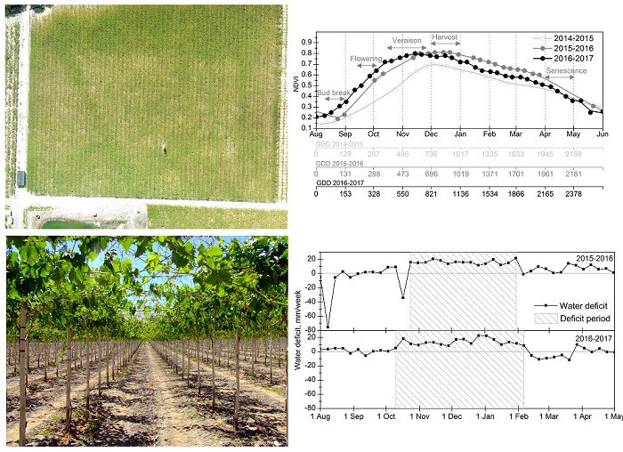
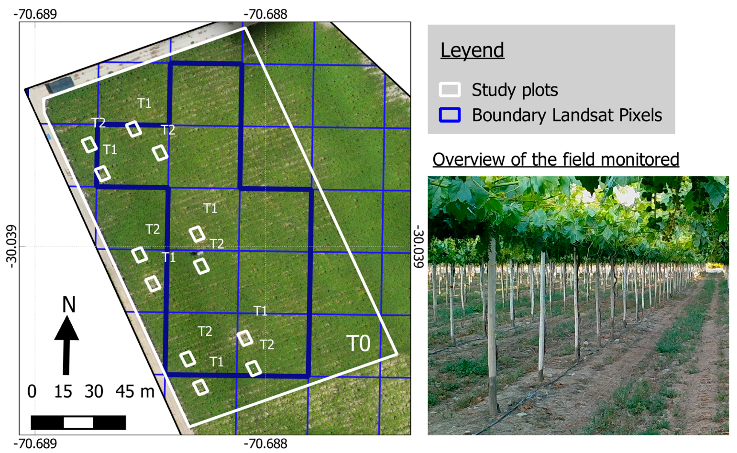
2.1. Study Site

The study was conducted during three growing seasons (2014–2015, 2015–2016, and 2016–2017) in a drip-irrigated table grape vineyard (cv. Flame seedless) located in the Elqui Valley, Coquimbo region, Chile (30°02′20″S, 70°41′17″W, 673 m above sea level) (Figure 1). The climate of the area is arid [19] and has an annual rainfall of approximately 100 mm concentrated in the winter months. The dry season lasts approximately 10–12 months. Therefore, the main hydrological feature of the area is periodic water scarcity due to the high inter-annual variation of rainfall and runoff. These patterns are strongly related to the El Niño Southern Oscillation (ENSO) [20]. The landscape is composed of irrigated agriculture concentrated along the river and sparse vegetation in the arid surrounding areas. The water for irrigation comes from surface reservoirs managed by the river water authority (Junta de Vigilancia del Río Elqui, Coquimbo region). The water authority delivers a water flow according with the water rights of the end users. Under water scarcity conditions, the water authority can reduce the flow of water released with the consequent reduction of the water received by the end users.
The average mean, maximum, and minimum annual temperatures during the experimental seasons were 16 °C, 26.2 °C, and 7.5 °C, respectively. The mean daily temperature ranges from approximately 12 °C in July to 21 °C in January (summer), with absolute maximum temperatures above 30 °C during the summer. The annual reference evapotranspiration (ETo, Penman Monteith) values were 1409, 1427, and 1461 mm for the 2014–2015, 2015–2016, and 2016–2017 growing seasons, respectively. The highest daily values of ETo, ranging from 6.0 to 6.8 mm, occurred in the summer (December and January). The soil is classified as loamy alluvial Entisol with flat topography (<1%) and moderate depth (>50 cm) [21]. The soil texture is sandy loam at the surface, sandy clay loam from 10 to 40 cm, and medium loam at depths greater than 40 cm. There are no limits to root development.
The experimental field was a commercial plot of 2.5 ha planted in 2012 with “Flame seedless” table grape vines on Harmony rootstock. Plants were trained on an overhead trellis system (2 × 3 m spacing, 1667 plants per ha), with an average plant height of 2 m. The vineyard agronomic management described by Ibacache et al. [21] was oriented toward increasing the yield, fruit size, and quality. The yield data for the 2015–2016 and 2016–2017 seasons are presented in Table 1. The irrigation system was a surface drip line with two emitters spaced at 1 m per plant (4 L h−1 per emitter). There was one pipeline per plant row. The precipitation during the experimental seasons was 59, 115, and 1 mm, respectively, and the irrigation depths applied by the farmer for these seasons are shown in Table 2. The irrigation was managed by the farmer during the experimental period. The farmer received irrigation advice based on the proposed approach (weekly values of net irrigation water requirements), but the real amount of irrigation was based on the availability of water in the network of canals and the irrigation requirements of other sectors of the farm. In addition, two irrigation treatments were introduced into the field: Treatment T1, where the irrigation dose was reduced by 25% with respect to the farm management, and Treatment T2, where the irrigation dose was increased by 25% with respect to the farm management. The main purpose of the treatments was the analysis of a possible increase of the yield quality and quantity increasing the irrigation dose or, alternatively, the demonstration of a possible improvement of the water productivity reducing the water applied. The treatments were implemented by changing the emitters in blocks of nine plants (3 × 3 plant array) with six replicates of each treatment in the plot (54 plants per treatment). The farm management is named T0. The amount of irrigation applied in each season is indicated in Table 2.

2.2. Ground Data

The ground data analyzed in this work include meteorological values from an agrometeorological station, midday stem water potential, the fraction of photosynthetic active radiation intercepted by the vines (fPAR), soil humidity evolutions, crop phenology (main stages), and harvest quantity and quality. The reference evapotranspiration (ETo) and precipitation were obtained using meteorological data from an automatic weather station located 0.8 km away from the experimental site (30°02′17.79″S, 70°41′47.55″W) belonging to a regional network of meteorological stations [22]. The daily ETo was calculated using the FAO-56 Penman–Monteith equation [6]. To evaluate the internal water status of the vines, the midday stem water potential (Ψx) was measured using a Scholander pressure chamber (PMS600, PMS Instruments Company, Corvallis, OR, USA). The measures were taken close to the time of the daily maximum vapor pressure deficit on fully-expanded leaves located near the principal branches of the plants. Selected leaves were saved in plastic bags covered with aluminum foil for 2 h before the measurement. The measurements were taken weekly from October to March during the growing seasons.
The experimental values of fPAR were measured on a biweekly basis for all of the treatments. A hand-held ceptometer (ACCUPAR LP-80, Decagon Devices, Inc., Pullman, WA, USA) was located facing the sky above, and below, it faced the plant canopy in 10 randomized positions within each block of irrigation treatment. The fPAR was estimated as the ratio between intercepted radiation (PAR above the canopy minus PAR below the canopy) over incoming PAR. The soil humidity was monitored at a depth of 20 cm during the whole growing season. The probes (GS1, Decagon Devices, Inc.) were buried 15 cm from the emitters in the central plant of each irrigation treatment. At harvest time (Table 1), the yield was evaluated in the central plant of each block (in the 3 × 3 array) of each irrigation treatment and was expressed as kg fruit ha−1. The same number of plants was harvested in the orchard for comparison. Average yield and fruit quality parameters (berry weight and equatorial diameter) were measured in the orchard and in each treatment. The ground data analyzed in this work corresponded mostly to the growing seasons 2015–2016 and 2016–2017 since the plants were immature during the first experimental growing season (2014–2015). The crop phenology was determined by direct observation.
The crop growth and development are presented in this work in terms of calendar dates and thermal time defined by the growing degree days (GDD). The GDD was calculated from 1 August based on the daily maximum and minimum air temperature and the function proposed by McMaster et al. [23]. The base temperature used in the formulation was 10 °C. The analyses of the significance of the differences for the parameters were based on ANOVA and Duncan tests.

2.3. Satellite Data

Irrigation performance was assessed using satellite images acquired by the Landsat 8 Operational Land Imager sensor (L8-OLI). The experimental plot is located in a two-path-row overlap zone (233-081 and 001-081), so the time series of satellite images acquired was useful in describing the temporal evolution of the canopy. The NDVI were calculated on a pixel-by-pixel basis from images provided by the USGS Global Visualization Viewer (https://glovis.usgs.gov/). The effect of the atmospheric distortion was compensated for by applying a normalization procedure based on pseudo-invariant surfaces [24]. The NDVI values obtained in each acquisition date were rescaled so the NDVI values obtained in the pseudo-invariant surfaces match the common values of NDVI in these areas. The pseudo-invariant surfaces were bare soil in agricultural plots and dense vegetation, like alfalfa; the known NDVI values for these surfaces are 0.18 and 0.91, based on field measurements in the area. If these surfaces were not available on a particular date, we applied a general equation derived for the previous time series. The NDVI was averaged for each acquisition date avoiding the pixels near the field edge. The selection of pixels avoiding the edge results in nine Landsat pixels (8100 m2). The effect of the treatments in the NDVI at field scale is reduced, considering the limited extension of the treatments (650 m2). A total number of 78 cloud-free images over the study area were used, with a minimum of 21 images per growing season and at least two images per month. The NDVI was linearly interpolated between the images acquisition dates to obtain daily values of the desired parameters in the analysis of irrigation performance. For the anticipation of the irrigation requirements, the NDVI data must be extrapolated as presented in Section 2.6.

2.4. Simplified Operational Approach to Net Irrigation Requirements

The net irrigation water requirement (NIWR) is the water that must be supplied by irrigation to satisfy the crop ET, leaching (if necessary), and miscellaneous water supply, such as run-off, that is not provided by water stored in the soil and precipitation that enters the soil [25]. Therefore, the calculation of NIWR requires the estimation of the components of the soil water balance (Equation (1)), where the negative terms refer to water inputs in the system (precipitation, P; variation of the soil water content, ΔS; and capillarity rise, CR) and the positive terms refer to water outputs (ETc; deep percolation, DP; and runoff, RO), all in mm:
I = ETc + DP + RO P Δ S CR
For agricultural fields in the study area, CR can be assumed to be zero because of the depth of the water table. In addition, RO was also assumed to be zero because of the characteristics of the irrigation system (drip irrigation) and the scarce precipitation registered during the study period. In this approach, the soil drains when the soil water content in the root zone exceeds field capacity. As long as the soil water content in the root zone is below the field capacity, the soil will not drain and DP is equal to 0. The analysis performed indicates that the soil layer never drains during the analyzed period. The term ΔS can be important at the beginning of the growing periods in some crops and climatic conditions. However, in the current conditions, the water accumulated in the soil profile at the beginning of the growing season represents less than 5% of the NIWR during the entire growing seasons. The precipitation accumulated during the dormancy period (from May to August) was always lower than 45 mm and more that the 80% is evaporated according to the model presented below. During the irrigation campaign, the irrigation recommendation tried to maintain ΔS equal to 0. Thus, the crop requirements are entirely covered by the irrigation plus precipitation and we attempted to avoid the accumulation of water in the soil profile. For the reason exposed, in this study the NIWR was estimated to be equal to ETc − P.

2.5. Estimation of Crop Transpiration

In applications of crop irrigation management, the strength of the reflectance-based crop coefficient models is the capability to estimate the potential crop transpiration. The relationship is generally established in terms of the basal crop coefficient or transpiration coefficient (Kcb) and the selected VI. Then, the soil evaporation coefficient (Ke) must be calculated by separately applying a daily soil water balance in the soil top layer, as proposed by Allen et al. [6] and Torres and Calera [26] (Equation (2)):
ETc = Kc × ETo = ( Kcb + Ke ) × ETo
A controversial point for the application of the Kcb-VI model is the selection of the most adequate relationship for the crop analyzed. However, based on our experience and the references listed in the literature review, some Kcb-VI relationships exhibit very good agreement for different crops. Melton et al. [27] proposed the use of a generalized relationship for real-time and operational purposes that enables its applications to crop-specific relationships a posteriori when information about crop architecture is available. In agreement with this line of thinking, several authors [17,28,29] concluded that some relationships developed for different crops are valid for the assessment of ETc in different crops and areas. Therefore, the relationship used in this work was the Kcb-NDVI relationship developed by Campos et al. [13] in an irrigated vineyard managed in vertical shoot-positioned trellises (Equation (3)) in the West of Spain (semi-arid area). This relationship was demonstrated to be similar to the Kcb-NDVI described by Bausch and Neale [30] for corn, and the same relationship has been demonstrated valid for the assessment of crop transpiration in several canopies and various climate conditions. In this sense, Campos et al. [16,31] demonstrated the aptitude of this relationship to estimate crop transpiration in row-vines in central Portugal and bush-vines in the West of Spain. Campos et al. [32,33] evaluated this relationship in Mediterranean savanna (natural vegetation) in the East of Spain. Hornbuckle et al. [28] concluded that this relationship reproduces the Kcb behavior for wine-grapes in Australia. Finally, Odi-Lara et al. [17] concluded that the relationship between the Kcb and the soil adjusted vegetation index for apple trees in the south of Chile was very similar to the relationship described by Campos et al. [13] using the same index. While the Kcb-NDVI relationship should be evaluated in more canopies and climate conditions, the evidence provided let us use the proposed relationship for real-time and operational purposes. In addition, and considering that the selection of the most adequate equation in operational application is an open question, we analyzed the use of the Equation (4), developed by Trout and Johnson [34] and routinely used in the IrriSatSMS system (Irrigation Water Management by Satellite and SMS) developed in Australia by CSIRO (Commonwealth Scientific and Industrial Research Organization):
Kcb = 1.44 × NDVI 0.1
Kcb = 1.37 × NDVI 0.086
As indicated above, the soil evaporation should be considered when estimating ETc. However, the estimation of this parameter requires a knowledge of the characteristic of the irrigation system and soil properties, as well as the irrigation frequency and doses on a daily scale, and these parameters are not always available in field applications. Considering the uncertainties estimating this coefficient, the NIWR analyzed in this work was based on the product of Kcb × ETo following other operative approaches, such as the Terrestrial Observation and Prediction System-Satellite Irrigation Management Support supported by NASA (TOP-SIMS, https://ecocast.arc.nasa.gov/simsi/about/). This formulation accounts for the plant transpiration and the residual soil evaporation [6]. However, the evaporation from the wet soil surface was estimated for the field monitored and the results were conveniently discussed. For a broad description of the soil evaporation model used in this work, the reader is referred to the FAO-56 Manual [6] and further modifications proposed by Torres and Calera [26]. The adaptation of this model using information derived from satellite images is described by Campos et al. [13]. Finally, the parameters needed for the application of this model in the analyzed field are the size of the wet bulb (30% of the surface), the depth of the soil layer where the evaporation occurs (0.05 m), and the soil texture in the top layer (sandy loam).

2.6. Application of the Model in Real-Time Irrigation Advice

The methodology is applied in real-time during the current campaign, providing irrigation advice in the study field. The information about crop transpiration is delivered weekly to the farmer so the irrigation schedule can be planned a week ahead. The information is provided in terms of “recommended time of irrigation” for the convenience of the end-user, and the farmer is advised about the necessity to discount the eventual precipitation from the estimated transpiration. The workflow basically consists of four simple steps: (1) The satellite images are downloaded and processed on the acquisition date. Landsat 8 images are downloaded from the Global Visualization System from the United States Geological Survey (GLOVIS-USGS, https://glovis.usgs.gov/). Although the analysis performed was mainly based on Landsat, the temporal evolution of the NDVI based on Sentinel was also considered since 2016. However, the density of Landsat images from 2016 and the low availability of cloud-free images from Sentinel prevent to the inclusion of these images in the present study. Sentinel 2 images are downloaded from the Copernicus Open Access Hub (https://scihub.copernicus.eu/); (2) The information is uploaded in Spider Web GIS (http://maps.spiderwebgis.org/login/?custom=default) for the visualization and the analysis of temporal series of satellite images [14]. The Spider Web GIS is updated after each image acquisition and contains the time series of color combinations and NDVI; (3) The temporal evolution of the NDVI for the study field is gathered from the system by specialized personnel and the Kcb values are computed; (4) Finally, the crop transpiration is estimated a week ahead based on the linear extrapolation of the Kcb based on the previous 3–4 images and the average ETo calculated for the same week during the previous growing seasons (three campaigns). The values derived from the linear extrapolation are limited to the maximum NDVI value obtained for the same crop in previous campaigns. The extrapolation and the use of historical ETo data could incur in deviations with respect to the measured data, as analyzed in this work. The current developments of the system include simpler approaches for the distribution of the estimated variables, including continuous maps of crop transpiration. However, the information is processed and analyzed manually in this case due to the importance of the experiment.

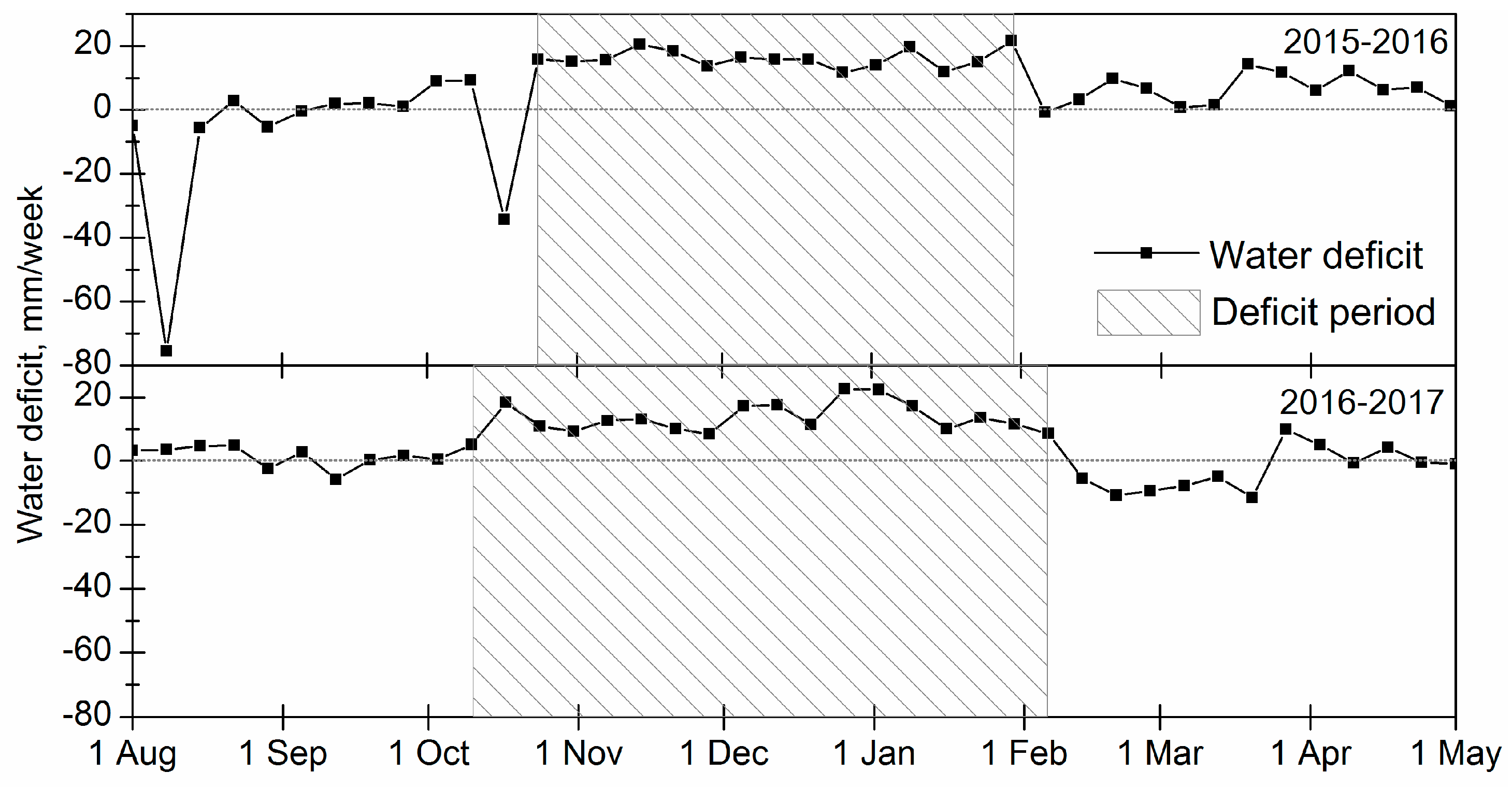
2.7. Estimation of Water Deficit

As presented in the introduction, a specific objective in this work is to evaluate the performance of the actual irrigation management against the NIWR estimated by the product Kcb × ETo minus the precipitation actually registered. This evaluation was performed at three time scales: weekly, monthly, and for the whole growing season. Consequently, the water deficit was estimated as the difference between NIWR and the irrigation actually applied. By the same definition, the deficit will be greater than 0 when the irrigation applied did not fulfill the crop requirements, and deficit values lower than 0 can be interpreted as an accumulation of water in the soil profile.

3. Results

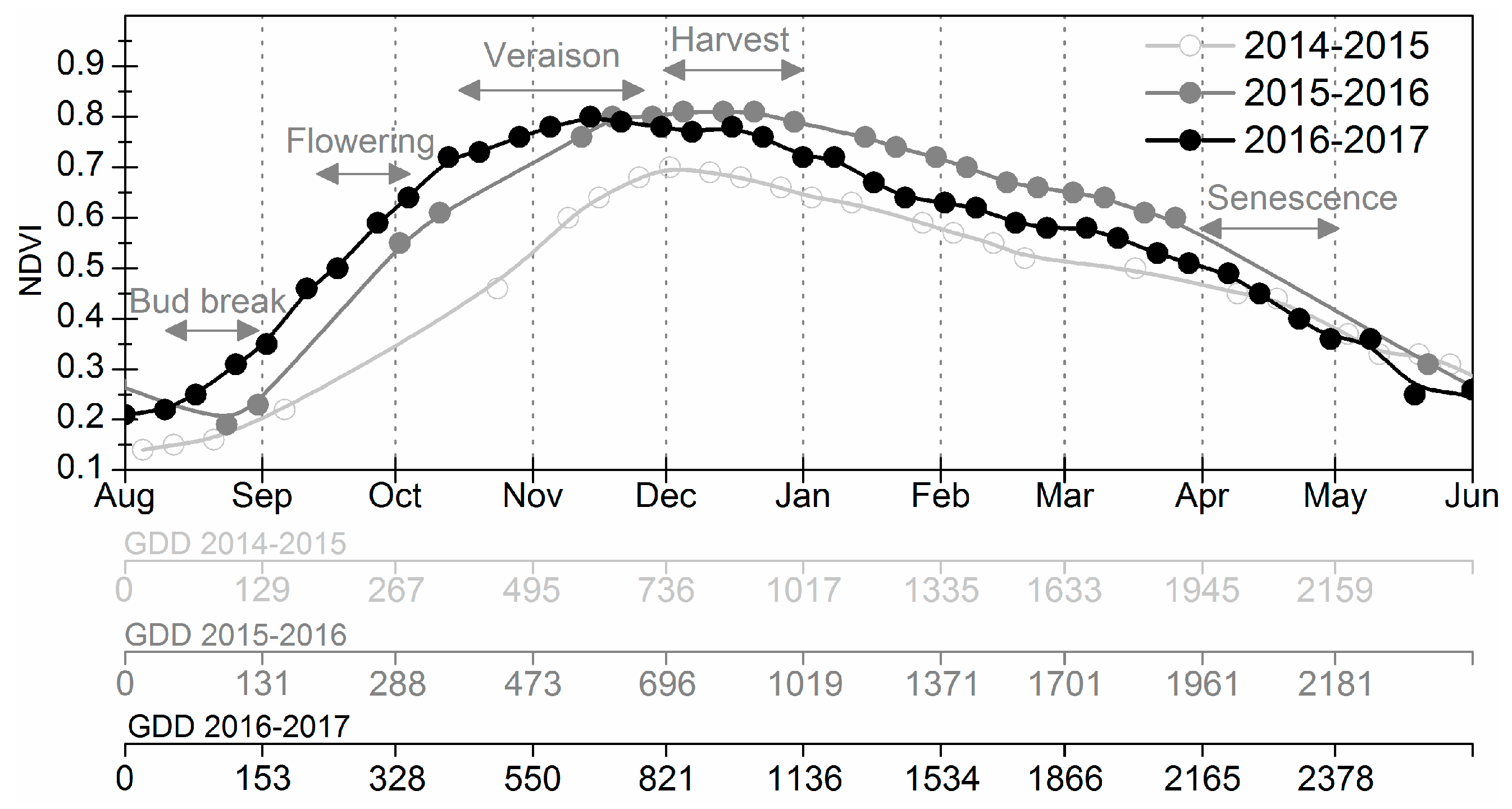
3.1. Characterization of Crop Growth, Yield, and Development

The evolution of the values of satellite NDVI clearly indicate up to four different growth phases for the growing seasons analyzed (Figure 2). These phases are similar to the crop development stages described in the FAO-56 manual for multiple crops [6]. The initial phase or stage corresponds to the bare soil conditions registered during July and the beginning of August, with NDVI values approximately 0.2 at the beginning of August. The second phase corresponds with the development stage and it is characterized by a fast increase in the NDVI, up to maximum values close to 0.85. The duration of this phase is approximately 500 GDD and occurred from August to November, depending on the analyzed campaign. The third phase corresponds to the mid stage and is a plateau period characterized by the relative stability of the NDVI around the maximum values. The length of the plateau is slightly lower than 500 GDD and, as indicated before, the exact dates and the duration in days depend on the analyzed growing season. In the analyzed campaigns this phase finished immediately after the harvest (December). The harvest dates and the average yield for the analyzed orchard and the treatments are presented in Table 1. The fourth phase corresponds with the maturity stage and was characterized by a slightly decreasing trend, followed by the senescence of the crop. The duration of this phase was different for each campaign monitored and the last phase finished after 2250 or 2500 GDD, depending on the analyzed campaign. In the analyzed campaigns, the crop reached bare soil values during late June. During the 2014–2015 season, the plants in the orchard were considered immature; consequently, the maximum NDVI values were substantially lower during the peak cover. Based on Equation (3), the minimum Kcb value estimated during the growing season was approximately 0.19, and the maximum Kcb, corresponding to the peak cover, was approximately 1.12 for the orchard at tree maturity. Based on Equation (4), the minimum and maximum Kcb values were 0.19 and 1.09.
Since the study was conducted in a young vineyard it was not possible to find significant differences among treatments for every evaluated parameter in the first season. However, from the second evaluating season (2015–2016), a clear influence of irrigation treatments (T0: regular management, T1: under-irrigation, and T2: over-irrigation) was found on vine vigor, measured as pruning weight (Table 1) and fPAR. The crop yield average obtained during two seasons did not register significant differences, but a significant negative effect of water restriction was found on yields in the second campaign. Compared to wine grape varieties, it is more difficult to have yield differences among irrigation treatments in table grape varieties because, in the last case, a crop adjustment is used to improve the fruit quality. The quality parameters (berry diameter and berry weight) obtained during the first and second analyzed campaigns (2014–2015 and 2015–2016) indicate a positive correlation with the water applied. The effect of the treatments in the quality parameters was not clear during the last analyzed campaign. The differences in the quality parameters were statistically significant for the average values obtained in each treatment during the whole study period (see Table 1).

3.2. Comparison of NIWR Based on Predicted and Measured Values of NDVI and ETo

The results of the model working in real-time indicated that the anticipation of the crop transpiration based on the average ETo from previous seasons and the extrapolation of the NDVI values could provide a precise estimation of the NIWR. Using Equation (3), the seasonal NIWR based on the extrapolated value was 669 mm in the 2014–2015 season, 940 mm in the 2015–2016 season, and 912 mm in the 2016–2017 season, without considering the precipitation. Using the same relationship, the seasonal NIWR based on the measured values of NDVI and ETo was 700 mm in the 2014–2015 season, 939 in the 2015–2016 season, and 925 mm in the 2016–2017 season. The root mean square error (RMSE) comparing the NIWR based on predicted and measured values was lower than 3.0 mm/week for every analyzed growing season. The maximum differences (7.7 mm/week) were obtained during late December and the beginning of January. The estimated values of the NIWR based on the extrapolated data of NDVI and the average ETo from previous seasons were provided to the farmer every week during the analyzed campaigns. However, the farmer followed the regular management based on the experience and the water availability as described before, incurring several periods of water shortage and over-irrigation, as analyzed in the next sub-section.

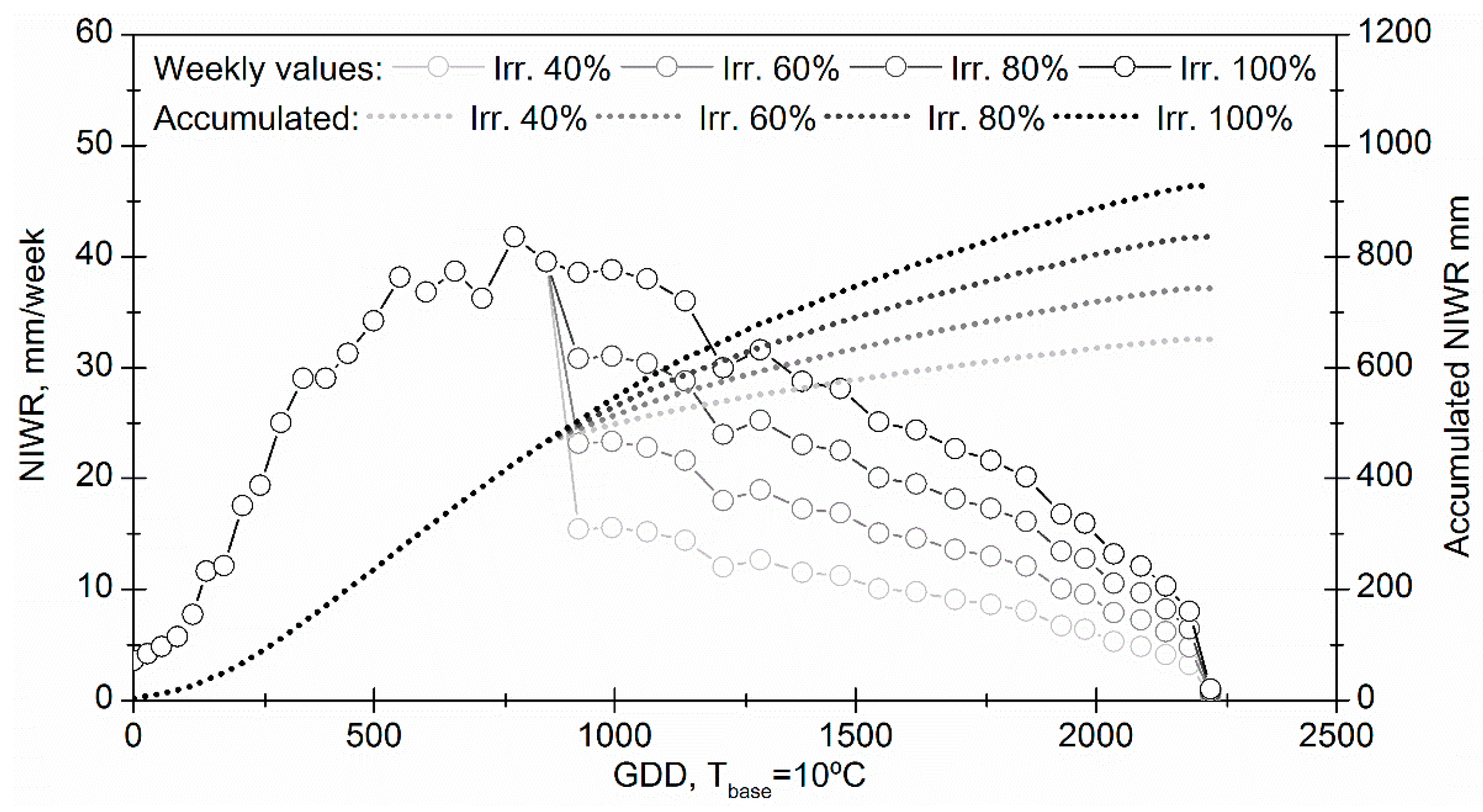
3.3. Comparison of Net Irrigation Water Requirements and Irrigation Applied

The irrigation volumes applied and the net irrigation water requirements are presented in Table 2 in terms of the values accumulated monthly. The NIWR simulated by the model based on Equation (3) is approximately 930 mm per growing season, without considering the precipitation registered during this period. The weekly values ranged from 5 to 42 mm/week, with December being the month with higher demand (40 mm/week on average). The total irrigation applied by the farmer (T0) is lower than the recommended volumes, with an average difference of about 200 mm during all of the campaigns analyzed. The precipitation registered during the seasons analyzed was important only during the 2014–2015 (59 mm) and 2015–2016 (115 mm) seasons. Then, the irrigation applied during the whole campaign (from August to April) for the regular management of the orchard (T0) is around 76% of the NIWR during all of the campaigns analyzed. For the analyzed field, the soil evaporation was estimated in 115 mm on average during all analyzed campaigns (less than 3.5 mm/week). The water used in evaporation should also be covered by the irrigation, so the regular management in the orchard is actually covering less than the 76% of the NIWR. However, the uncertainties of the soil evaporation model and the impossibility to estimate this variable in real time applications prevent the use of this coefficient as discussed below.
In addition to the differences observed in terms of the total amounts, the analysis of the monthly volumes of irrigation revealed several periods of water shortage. During all of the campaigns analyzed, the irrigation applied fit the NIWR well only from August to September. From October to January, the NIWR were not satisfied in any of the campaigns analyzed. Finally, the farmer tended to over-irrigate from February to March. Therefore, the deficit of water from October to January resulted in a plant water deficit, although the precipitation registered during the second growing season (2015–2016) could attenuate the deficit on this campaign. These deficits were corroborated through the stem water potential measurements presented in the next subsection.
The analysis of the water deficit at weekly time-scale corroborates the differences found for the monthly accumulated values. The periods with continuous deficits occurred from late October to late January during the 2015–2016 season and from mid-October to mid-February during the next growing season (Figure 3). The precipitation registered during the spring and winter of 2015 resulted in a negative deficit that can be interpreted as the recharge of the soil profile. The recharge was estimated to be approximately 110 mm and could be stored in the soil profile, thus providing additional resources for the plants during this growing season. The regular management resulted in negative deficits during the period when the vegetation vigor decreased (after harvest) during the 2016–2017 season. In general terms, the deficit was zero or greater during the crop senescence.

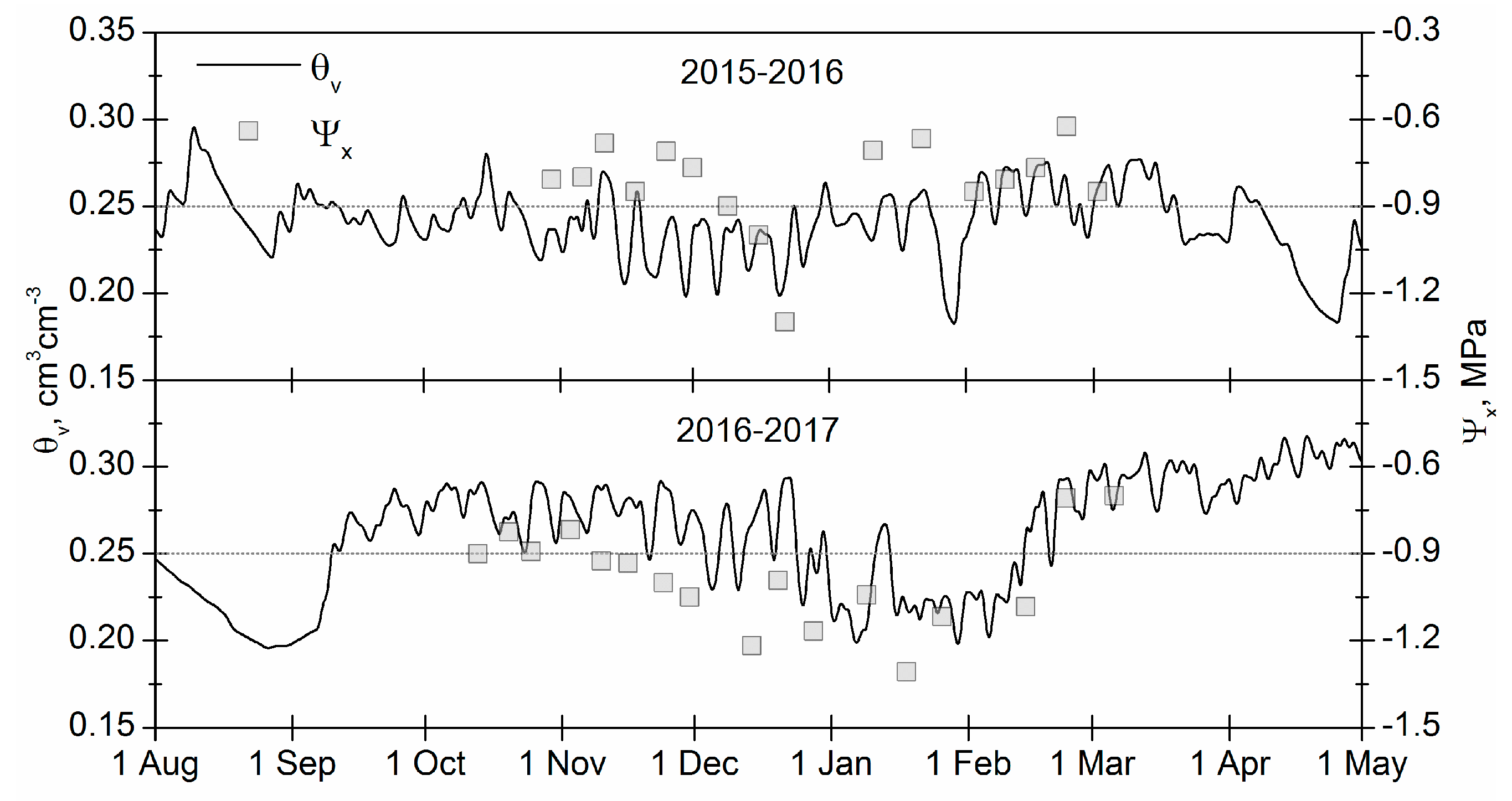
3.4. Evaluation of the Internal Plant Water Status

The analysis of the stem water potential (Ψx) measured during the 2015–2016 season did not reveal any significant trend. However, the Ψx values indicate a period of water shortage during December reaching minimum values of approximately −1.3 MPa on 22 December 2015 (Figure 4). During the next growing season, 2016–2017, the Ψx values indicate that the three phases were clearly differentiated (Figure 4). During October and the beginning of November, the values of Ψx remained relatively stable with the minimum value being approximately −0.9 MPa. The second phase, from November to February, was characterized by a clear decreasing trend with the minimum values lower than −1.3 MPa on 18 January 2017. After this period, the increase in the irrigation applied promoted the accumulation of water in the soil profile (Figure 4), and the plants reached the same values of Ψx that were registered at the beginning of the growing season. The plant’s internal turgor was higher during the 2015–2016 season, although the soil humidity at 20 cm was lower during this campaign (Figure 4). This apparent discordance could be explained by the accumulation of water in the deepest soil layers as analyzed in the discussion section. The stem water potential (Ψx) for the 2015–2016 and 2016–2017 seasons are presented in Table 3.

4. Discussion

The phases described for the NDVI curves in this experiment were similar to the stages described by Er-Raki et al. [12] for Kc and NDVI curves for table grapes cv. Superior and cv. Perlet in Mexico. The main difference in the NDVI curves reported by these authors is the maximum NDVI obtained in both experiments (0.7 versus 0.85). The maximum Kcb obtained in this work is greater than the Kcb proposed in the FAO-56 manual [6] for table grape (Kcb = 0.8). The shape of the curve and the maximum Kcb value reported in this study were similar to the Kc curve reported by Vanino et al. [35] from bud-break to harvest in table grape vineyards trained on an overhead trellis system, called “tendone” in Italy. The differences in the maximum values of NDVI or Kcb obtained in the different experiments, as well as the multiannual variability described in this work, reinforce the necessity of feasible approaches based on field data to describe the actual crop coefficient (in situ) and the water requirements for the crop analyzed. In the same vein, the proposed approach could provide valuable information for the assessment of irrigation necessities as proposed in previous experiments [10,17,29]. In addition, the availability of satellite images and the accessibility of using the most recent developments [14] allow operative applications, as presented in this study. The routine use of Sentinel 2A and Sentinel 2B increments the temporal and spatial resolutions providing up to two images per week in the study area with a spatial resolution greater than 100 m2 (0.01 ha). In addition to this, the compatibility of the NDVI derived from Landsat 8 and Sentinel 2 [36] simplified the calculation procedures. A virtual constellation based on Landsat 8 and Sentinel 2 is being applied during the current campaign of irrigation advice.
The analysis provided demonstrated the possibility to anticipate the NIWR based on the extrapolation of the NDVI values and the average ETo from previous season. The methodology is subjected to the obvious uncertainty of the extrapolation approach and the variability in the weather conditions. However, the differences obtained were lower than 8 mm/week, and the greater differences were registered during late December and the beginning of January. During these dates, the NIWR were estimated at about 40 mm/week, so the maximum difference corresponded to 19% of NIWR. The maximum differences were obtained for the weeks when the ETo presented sudden variations with respect to the average values. These differences point to the necessity to consider the actual weather conditions, including prognostic values, such as the maximum and minimum temperatures forecast provided by several agencies at various scales. In addition, the possible deviations can be detected and mitigated during the next irrigation event, but this strategy was not followed in this experiment considering the contrasted differences between the NIWR recommendation and the farmer management.
According to the water deficit analysis, the irrigation applied in the analyzed seasons was insufficient to satisfy the plant’s requirements, and the deficit periods coincided with low values of stem water potentials and decreases in soil moisture measurements. These results point to the necessity to increase the total volumes applied and the improvement of the temporal distribution of the irrigation applied. The stem water potential measured at the beginning of the growing season was within the ranges of well-irrigated table grapes obtained by Mabrouk [4] and Conesa et al. [3], but these values descend to the minimum values that have been described as an indicator of water stress by these authors. In contrast, the irrigation applied in the treatment T2 roughly match the NIWR simulated by the model from bud-break to harvest during both analyzed campaigns. This increment in the irrigation doses increased the yield (Kg/ha) by 11% and quality (2% berry diameter and 6% berry weight) in T2 with respect to T0 (Table 1). The field data suggested a positive trend comparing yield and quality data with respect to the water applied. However, the differences in grape quality were not statistically significant for every single analyzed campaign. During the 2016–2017 season, the berry diameter and weight were lower in the treatment T0 in comparison with the treatment T1. We interpret that the low production registered in the T1 during this campaign improved the grape quality in comparison with the treatment T1. The berry diameters obtained in the treatment T2 were similar to, or even greater than, the diameters reported by Ruiz et al. [37], using different mulch treatments, and Ibacache et al. [21], who selected different rootstocks in the same region for cv. Flame.
The increment of irrigation also positively influences the canopy development by 7% in the maximum cover (see the fPAR column in Table 1). We hypothesized that these differences were more evident during the last season analyzed, because the precipitation registered during the winter (69 mm) and spring (45 mm) of 2015–2016 recharged the soil profile, maintaining the soil humidity in the deepest layers. The water accumulated on these layers moderated the differences in water availability between the treatments, reduced the difference in the maximum fPAR values and delayed the descending trend of Ψx. Despite the fact that opposing relationships between canopy growth (related with pruning weight) and yield have been described in previous experiments for table grape [38], we did not identify these effects in the present study. These considerations reinforce the necessity to increase the irrigation doses, primarily during the period from bud-break to harvest.
The NIWR simulated by the model based on the Equation (3) is approximately 930 mm per growing season, without considering the precipitation registered during this period. The total seasonal transpiration based on the Equation (4) was 911 mm during the 2015–2016 season and 918 mm during the season 2016–2017. The RMSE comparing the NIWR based on the Equations (3) and (4) was lower than 1.6 mm/week, demonstrating the similitude between both approaches. The modeled NIWR is within the range of irrigation requirements estimated by Zuñiga et al. [8], who measured the shaded area beneath the canopy in the same table grape variety in central Chile, but it is slightly lower than the irrigation requirements estimated by Er-Raki et al. [12] for different varieties in Northern Mexico (1100 mm). However, and as indicated in the methodology, this estimation of NIWR only considers plant transpiration, so it should be increased for the evaporation component depending on the soil type, irrigation frequency, and characteristics of the irrigation system. The soil evaporation was estimated in about 115 mm per growing season in the study field, equivalent to a 15% of the NIWR. This value was not included in the NIWR since the irrigation frequency and doses must be considered unknown in real-time applications, providing irrigation advice a week ahead. In addition, several authors were alerted about the partitioning between crop transpiration and soil evaporation based on the FAO-56 approach since the Kcb-NDVI relationship already includes a residual soil evaporation [29], and the depth of the evaporative soil layer could be overestimated [26].
As indicated in the description of the study site description, the study area and the whole northern part of Chile are subjected to long periods of low availability of water resources (drought). During these periods, irrigation cannot adequately cover the NIWR. Under these conditions, the proposed methodology can provide a quantitative guideline for the design of deficit irrigation strategies. The possible alternatives of deficit irrigation are the induction of water stress at different phenological stages before harvest or the application of deficit irrigation after harvest. In the table grape crops, the application of deficit irrigation before harvest could result in a reduction of the yield quantity and quality [4,39] if the extent and the intensity of the water deficit is not controlled. Conversely, the effects of postharvest irrigation deficit have not been extensively analyzed in table grapes, but the application of this strategy shows beneficial effects [40] in wine grapes. In the same vein, Myburg [41] reported that the water deficits during the postharvest period have no significant effect on cane starch content, considered as an indicator or reserve accumulation, after four years of deficit treatment in raisin grapes (cv. Sultanina). Based on these findings, we propose a pre-season irrigation guidance based on the model and considering three levels of deficit irrigation after harvest (Figure 5). The results modeled indicate that the irrigation should decrease from 930 mm to 835 mm for the reduction to 80%, 743 mm for the reduction to 60%, and to 630 mm for the most restrictive scenario. These scenarios did not consider the eventual precipitation, which should be discounted from NIWR, and the general guidance should be revised in real-time with actual NDVI and ETo data. However, the effects of these strategies in the reserve accumulation on roots should also be analyzed. Very restrictive schemes, such as the replacement of the 25% of ETc after harvest, have been shown to deleteriously affect yield and yield quality in other species, such as peach trees [42].

5. Conclusions

The information provided by the proposed approach can improve the regular management of crop irrigation based on the experience of the farmer and the water availability. This methodology is based exclusively on satellite and meteorological records, and both datasets are currently available in the area from open sources. The availability of the data and the robustness of the methodology applied allow the analysis of the irrigation performance at the scale of a commercial field, providing quantitative valuable information for irrigation management, such as identifying the periods of water shortage and over-irrigation.
The data analyzed in this work indicate that the irrigation timing should be improved in the field studied, mostly before harvest. The analysis of the ground data for different irrigation treatments (internal plant water status, vegetative development, productivity) corroborates this conclusion and indicates that an adequate distribution of the irrigation, following the proposed approach, can promote the crop’s productivity in terms of yield quantity and quality.
It is important to note that the proposed approach can be used to design irrigation strategies to improve the yield and yield quality, but, in addition, this method can be used to define deficit strategies in times of low water availability. The application of this irrigation strategy will be evaluated in future growing seasons and we will analyze the impact of the deficit irrigation in the plant longevity in a long-term experiment. The irrigation advice, independent of the strategy selected, can be based on a standardized approach adapted to the actual crop growth and meteorological conditions.
The proposed methodology allows an initial diagnosis of irrigation performance before approaching the real conditions in the field. For this reason, because remote sensing can be utilized to widely view the area, it is an ideal method for institutions to use to provide advice on irrigation over a large territory. We strongly recommend the definition of general pre-season guidance and the estimation of field-based weekly advice.

Acknowledgments

This work was carried out as part of the CONICYT-FONDECYT Project “Orchards of the future: monitoring and definition of grape vineyard water status oriented to improve the irrigation management efficiency”; Cod. 11140843, funded by the Chilean government. Isidro Campos and Alfonso Calera were supported by the projects HERMANA (HERramientas para el MAnejo sostenible de fertilización Nitrogenada y Agua), funded by the Spanish Ministry Science and Innovation (AGL2015-68700-R), and FATIMA (FArming Tools for external nutrient Inputs and water Management), funded by the European Union's Horizon 2020 research and innovation programme (Grant Agreement No. 633945). We dedicate this work to the memory of our beloved friend Nicolás Franck Berger, a great scientist and a great person in life.

Author Contributions

Claudio Balbontín led the design and implementation of the field experiments and the redaction of the manuscript; Isidro Campos and Magali Odi contributed to the satellite crop monitoring and to the interpretation of the results. Antonio Ibacache designed and supervised the yield quality assessment, and Alfonso Calera contributed with his experience in the subject of the manuscript. All the authors contributed to the redaction of the manuscript.

Conflicts of Interest

The authors declare no conflict of interest.

References

  1. ODEPA Oficina de Estudios y Políticas Agrarias. Estadísticas Agrarias. Available online: http://www.odepa.gob.cl/estadisticas/productivas/ (accessed on 1 October 2017).
  2. Du, T.; Kang, S.; Zhang, J.; Li, F.; Yan, B. Water use efficiency and fruit quality of table grape under alternate partial root-zone drip irrigation. Agric. Water Manag. 2008, 95, 659–668. [Google Scholar] [CrossRef]
  3. Conesa, M.R.; Torres, R.; Domingo, R.; Navarro, H.; Soto, F.; Pérez-Pastor, A. Maximum daily trunk shrinkage and stem water potential reference equations for irrigation scheduling in table grapes. Agric. Water Manag. 2016, 172, 51–61. [Google Scholar] [CrossRef]
  4. Mabrouk, H. The use of water potentials in irrigation management of table grape grown under semiarid climate in Tunisia. OENO One 2014, 48, 123–133. [Google Scholar] [CrossRef]
  5. Chaves, M.M.; Zarrouk, O.; Francisco, R.; Costa, J.M.; Santos, T.; Regalado, A.P.; Rodrigue, M.L.; Lopes, C.M. Grapevine under deficit irrigation: Hints from physiological and molecular data. Ann. Bot. 2010, 105, 661–676. [Google Scholar] [CrossRef] [PubMed]
  6. Allen, R.G.; Raes, D.; Smith, M. Crop Evapotranspiration: Guidelines for Computing Crop Requirements; FAO Irrigation and Drainage Paper 56; Food and Agriculture Organization of the United Nations (FAO): Rome, Italy, 1998. [Google Scholar]
  7. Williams, L.E.; Ayars, J.E. Grapevine water use and the crop coefficient are linear functions of the shaded area measured beneath the canopy. Agric. For. Meteorol. 2005, 132, 201–211. [Google Scholar] [CrossRef]
  8. Zuñiga, C.; Aspillaga, C.; Ferreyra, R.; Selles, G. Response of “Flame Seedless” vines to different levels of irrigation water in the Aconcagua Valley, Chile. Acta Hortic. 2017, 1150, 295–302. [Google Scholar] [CrossRef]
  9. Neale, C.; Bausch, W.; Heerman, D. Development of reflectance-based crop coefficients for corn. Trans. ASAE 1989, 32, 1891–1899. [Google Scholar] [CrossRef]
  10. Hunsaker, D.J.; Pinter, P.J.; Barnes, E.M.; Kimball, B.A. Estimating cotton evapotranspiration crop coefficients with a multiespectral vegetation index. Irrig. Sci. 2003, 22, 95–104. [Google Scholar] [CrossRef]
  11. Gonzalez-Dugo, M.P.; Neale, C.M.U.; Mateos, L.; Kustas, W.P.; Prueger, J.H.; Anderson, M.C.; Li, F. A comparison of operational remote sensing-based models for estimating crop evapotranspiration. Agric. For. Meteorol. 2009, 149, 1843–1853. [Google Scholar] [CrossRef]
  12. Er-Raki, S.; Rodriguez, J.C.; Garatuza-Payan, J.; Watts, C.J.; Chehbouni, A. Determination of crop evapotranspiration of table grapes in a semi-arid region of Northwest Mexico using multi-spectral vegetation index. Agric. Water Manag. 2013, 122, 12–19. [Google Scholar] [CrossRef]
  13. Campos, I.; Neale, C.; Calera, A.; Balbontin, C.; González-Piqueras, J. Assesing satellite-based basal crop coefficients for irrigated grapes (Vitis vinifera L.). Agric. Water Manag. 2010, 98, 45–54. [Google Scholar] [CrossRef]
  14. Calera, A.; Campos, I.; Osann, A.; D’Urso, G.; Menenti, M. Remote Sensing for Crop Water Management: From ET Modelling to Services for the End Users. Sensors 2017, 17, 1104. [Google Scholar] [CrossRef] [PubMed]
  15. Samani, Z.; Bawazir, A.S.; Bleiweiss, M.; Skaggs, R.; Longworth, J.; Tran, V.D.; Pinon, A. Using remote sensing to evaluate the spatial variability of evapotranspiration and crop coefficient in the lower Rio Grande Valley, New Mexico. Irrig. Sci. 2009, 28, 93–100. [Google Scholar] [CrossRef]
  16. Campos, I.; Balbontin, C.; González-Piqueras, J.; González-Dugo, M.P.; Neale, C.; Calera, A. Combining water balance model with evapotranspiration measurements to estimate total available water soil water in irrigated and rain-fed vineyards. Agric. Water Manag. 2016, 165, 141–152. [Google Scholar] [CrossRef]
  17. Odi-Lara, M.; Campos, I.; Neale, C.M.U.; Ortega-Farias, S.; Poblete-Echeverria, C.; Balbontin, C.; Calera, A. Estimating evapotranspiration of an apple orchard using a remote sensing-based soil water balance. Remote Sens. 2016, 8, 253. [Google Scholar] [CrossRef]
  18. Hunsaker, D.J.; Pinter, P.R., Jr.; Kimball, B.A. Wheat basal crop coefficients determined by normalized difference vegetation index. Irrig. Sci. 2005, 22, 95–104. [Google Scholar] [CrossRef]
  19. Kalthoff, N.; Fiebig-Wittmaack, M.; Meißner, C.; Kohler, M.; Uriarte, M.; Bischoff-Gauß, I.; Gonzales, E. The energy balance, evapo-transpiration and nocturnal dew deposition of an arid valley in the Andes. J. Arid Environ. 2006, 65, 420–443. [Google Scholar] [CrossRef]
  20. Fiebig-Wittmaack, M.; Astudillo, O.; Wheaton, E.; Wittrock, V.; Perez, C.; Ibacache, A. Climatic trends and impact of climate change on agriculture in an arid Andean valley. Clim. Chang. 2012, 111, 819–833. [Google Scholar] [CrossRef]
  21. Ibacache, A.; Albornoz, F.; Zurita-Silva, A. Yield responses in Flame seedless, Thompson seedless and Red Globe table grape cultivars are differentially modified by rootstocks under semi arid conditions. Sci. Hortic. (Amst.) 2016, 204, 25–32. [Google Scholar] [CrossRef]
  22. INIA Red Agrometeorológica del INIA. Available online: http://agromet.inia.cl/estaciones.php (accessed on 1 September 2017).
  23. McMaster, G.S.; Smika, D.E. Estimation and evaluation of winter wheat phenology in the central Great Plains. Agric. For. Meteorol. 1988, 43, 1–18. [Google Scholar] [CrossRef]
  24. Chen, X.; Vierling, L.; Deering, D. A simple and effective radiometric correction method to improve landscape change detection across sensors and across time. Remote Sens. Environ. 2005, 98, 63–79. [Google Scholar] [CrossRef]
  25. Jensen, M.E.; Burman, R.D.; Allen, R.G. Evapotranspiration and Irrigation Water Requirements; American Society of Civil Engineers: New York, NY, USA, 1990; Volume 1. [Google Scholar]
  26. Torres, E.A.; Calera, A. Bare soil evaporation under high evaporation demand: A proposed modification to the FAO-56 model. Hydrol. Sci. J. 2010, 55, 303–315. [Google Scholar] [CrossRef]
  27. Melton, F.S.; Johnson, L.F.; Lund, C.P.; Pierce, L.L.; Michaelis, A.R.; Hiatt, S.H.; Guzman, A.; Adhikari, D.D.; Purdy, A.J.; Rosevelt, C.; et al. Satellite irrigation management support with the terrestrial observation and prediction system: A framework for integration of satellite and surface observations to support improvements in agricultural water resource management. IEEE J. Sel. Top. Appl. Earth Obs. Remote Sens. 2012, 5, 1709–1721. [Google Scholar] [CrossRef]
  28. Hornbuckle, J. Vineyard Irrigation—Delivering Water Savings through Emerging Technology. In Final Report to Grape and Wine Research & Development Corporation; CSIRO Land and Water: Canberra, Australia, 2014; Available online: https://www.wineaustralia.com/getmedia/6e7c3e92-c36c-4685-9bf8-9039d99aa4a0/CSL-0901-Final-Report-IrriSAT (accessed on 8 December 2017).
  29. Campos, I.; Neale, C.; Suyker, A.; Arkebauer, T.; Gonçalves, I. Reflectance-based crop coefficients REDUX: For operational evapotranspiration estimates in the age of high producing hybrid varieties. Agric. Water Manag. 2017, 187, 140–153. [Google Scholar] [CrossRef]
  30. Bausch, W.C.; Neale, C.M.U. Crop coefficients derived from reflected canopy radiation—A concept. Trans. ASAE 1987, 30, 703–709. [Google Scholar] [CrossRef]
  31. Campos, I.; Calera, A.; Balbontin, C.; Torres, E.A.; González-Piqueras, J.; Neale, C.M.U. Basal crop coefficient from remote sensing assessment in rain-fed grapes in southeast Spain. In Remote Sensing and Hydrology; IAHS: Jackson Hole, WY, USA, 2010; Volume 352, pp. 397–400. [Google Scholar]
  32. Campos, I.; Villodre, J.; Carrara, A.; Calera, A. Remote sensing-based soil water balance to estimate Mediterranean holm oak savanna (dehesa) evapotranspiration under water stress conditions. J. Hydrol. 2013, 494, 1–9. [Google Scholar] [CrossRef]
  33. Campos, I.; Gonzalez-Piqueras, J.; Carra, A.; Villodre, J.; Calera, A. Calibration of the soil water balance model in terms of total available water in the root zone for a continuous estimation of surface evapotranspiration in Mediterranean dehesa. J. Hydrol. 2016, 534, 427–439. [Google Scholar] [CrossRef]
  34. Trout, T.J.; Johnson, L.F. Estimating crop water use from remotely sensed NDVI, Crop Models and Reference ET. In The Role of Irrigation and Drainage in a Sustainable Future, Proceedings of the USCID Fourth International Conference on Irrigation and Drainage, Sacramento, CA, USA, 3–6 October 2007; Clemmens, A.J., Anderson, S., Eds.; Colorado State University: Fort Collins, CO, USA, 2007. [Google Scholar]
  35. Vanino, S.; Pulighe, G.; Nino, P.; De Michele, C.; Bolognesi, S.F.; D’Urso, G. Estimation of Evapotranspiration and Crop Coefficients of Tendone Vineyards Using Multi-Sensor Remote Sensing Data in a Mediterranean Environment. Remote Sens. 2015, 7, 14708–14730. [Google Scholar] [CrossRef] [Green Version]
  36. Flood, N. Comparing Sentinel-2A and Landsat 7 and 8 using surface reflectance over Australia. Remote Sens. 2017, 9, 659. [Google Scholar] [CrossRef]
  37. Ruiz, R.; Sellés, G.; Ahumada, R. Aspectos físicos del suelo y calidad de fruta en parronales de uva de mesa. In Manejo de Riego y Suelo en Vides Para Vino y Mesa; Muñoz, I., Gonzalez, M., Sellés, G., Eds.; Instituto de Investigaciones Agropecuarias INIA: Santiago, Chile, 2007; pp. 77–84. [Google Scholar]
  38. Sommer, K.J.; Clingeleffer, P.R.; Ollat, N. Effects of minimal pruning on grapevine canopy development, physiology and cropping level in both cool and warm climates. Wein-Wiss. 1993, 48, 135–139. [Google Scholar]
  39. Faci, J.M.; Blanco, O.; Medina, E.T.; Martínez-Cob, A. Effect of post veraison regulated deficit irrigation in production and berry quality of Autumn Royal and Crimson table grape cultivars. Agric. Water Manag. 2014, 134, 73–83. [Google Scholar] [CrossRef]
  40. Behboudian, M.H. Zora Singh Water relations and irrigation scheduling in grapevine. Hortic. Rev. 2001, 27, 189–225. [Google Scholar]
  41. Myburgh, P.A. Responses of Vitis vinifera L. cv. Sultanina to water deficits during various pre- and post-harvest phases under semi-arid conditions. S. Afr. J. Enol. Vitic. 2003, 24, 25–33. [Google Scholar] [CrossRef]
  42. Wang, D.; Gartung, J. Infrared canopy temperature of early-ripening peach trees under postharvest deficit irrigation. Agric. Water Manag. 2010, 97, 1787–1794. [Google Scholar] [CrossRef]
Figure 1. Experimental plot with irrigation treatments distribution, boundary of Landsat pixels, and overview of the plants in the field.
Remotesensing 09 01276 g001
Figure 2. Evolution of the satellite normalized differences vegetation index (NDVI) values with respect to the calendar dates (upper graph). The accumulated value of growing degree-days (GDD) at the beginning of each month are presented for the monitored growing seasons (lower axis). The GDDs were calculated for a base temperature of 10 °C. The arrows indicate the main phenological stages.
Remotesensing 09 01276 g002
Figure 3. Weekly evolution of the water deficit estimated by the difference between farmer irrigation management and the modeled net irrigation water requirements (NIWR). A water deficit lower than 0 indicates over-irrigation and a water deficit greater than 0 indicates under-irrigation.
Remotesensing 09 01276 g003
Figure 4. Temporal evolution of soil water content (θv) measured at a depth of 20 cm and stem water potential (Ψx) in farmer irrigation treatment (T0). Absolute values below −0.9 MPa and descending trends in Ψx indicate water deficit conditions.
Remotesensing 09 01276 g004
Figure 5. Temporal evolution of the net irrigation water requirements (NIWR) and seasonal accumulated values based on three strategies of deficit irrigation after harvest.
Remotesensing 09 01276 g005
Table 1. Harvest date (HD), yield data (Y), berry diameter (BD), berry weight (BW), maximum fraction of photosynthetic active radiation intercepted by the vines (fPAR), and pruning weight per plant (PW) for the orchard monitored and the treatments induced in the field (T0, regular management of the orchard; T1, under-irrigation; and T2, over-irrigation). The significance of the differences (Sig.) was analyzed for each monitored campaign and for the average data. ND denotes “No Data”.
2014–2015
HD: 15 December 2014
2015–2016
HD: 22 December 2015
2016–2017
HD: 6 December 2016
Average
T1T0T2Sig.T1T0T2Sig.T1T0T2Sig.T1T0T2Sig.
Y (Ton/ha)NDNDNDND22.320.522.5NS17.7b21.8a24.5a5%20.021.223.5NS
BD (cm)18.518.818.9NS18.919.119.7NS19.919.820.1NS19.1b19.2ab19.6a5%
BW (g)3.33.53.6NS3.43.73.9NS4.14.04.2NS3.6b3.7a3.9a1%
fPARNDNDNDND0.770.800.85ND0.610.780.85ND0.690.790.85ND
PW (Kg)1.62.12.7NS2.4b3.2ab3.8a5%1.5c3.0b3.9a1%1.8c2.8b3.4a1%
Table 2. Monthly accumulated values of the net irrigation water requirements (NIWR), precipitation (P), and irrigation applied by the farmer for the whole field (T0) and the treatments established (T1 and T2).
Month2014–20152015–20162016–2017
Irrigation
(T1; T0; T2) mm/month
NIWR (P)
mm/month
Irrigation
(T1; T0; T2) mm/month
NIWR (P)
mm/month
Irrigation
(T1; T0; T2) mm/month
NIWR (P)
mm/month
August13; 17; 211127; 36; 45−49 (69)7; 10; 1221
September18; 24; 3011 (19)35; 47; 594645; 60; 7559
October33; 44; 556935; 47; 5954 (45)60; 80; 100125
November39; 52; 6511757; 76; 9515086; 114; 143158
December56; 74; 9314691; 121; 15218574; 98; 123175 (1.3)
January72; 96; 12012868; 91; 114169 (0.4)62; 83; 103149
February79; 106; 1328976; 101; 12612286; 115; 144105
March47; 62; 7830 (40)49; 65; 829679; 105; 13285
April5; 6; 84015; 20; 2551 (0.6)30; 39; 4947
Total (mm)361; 481; 601642453; 603; 754824529; 705; 882924
Table 3. Stem water potential (Ψx) and standard deviation values (SD) measured before harvest (T0, regular management of the orchard; T1, under-irrigation; T2, over-irrigation).
Growing SeasonStem Water Potential, Ψx
MPa (DS)
DateT1T0T2
2015–201630 October 2015−0.82 (0.19)−0.81 (0.09)−0.83 (0.15)
6 November 2015−0.62 (0.08)−0.80 (0.18)−0.70 (0.13)
11 November 2015−0.77 (0.08)−0.68 (0.05)−0.68 (0.09)
18 November 2015−0.92 (0.06)−0.85 (0.17)−0.77 (0.10)
25 November 2015−0.85 (0.10)−0.71 (0.16)−0.87 (0.16)
1 December 2015−0.92 (0.18)−0.77 (0.20)−0.82 (0.10)
9 December 2015−1.02 (0.28)−0.90 (0.15)−0.78 (0.17)
16 December 2015−1.20 (0.17)−1.00 (0.11)−1.02 (0.04)
22 December 2015−1.42 (0.10)−1.30 (0.06)−1.18 (0.13)
2016–201713 October 2016−1.03 (0.13)−0.90 (0.07)−0.87 (0.09)
20 October 2016−1.05 (0.11)−0.83 (0.13)−0.86 (0.08)
25 October 2016−0.98 (0.04)−0.89 (0.09)−0.85 (0.05)
3 November 2016−1.02 (0.04)−0.82 (0.13)−0.79 (0.05)
10 November 2016−1.05 (0.06)−0.93 (0.08)−0.81 (0.17)
16 November 2016−1.02 (0.11)−0.93 (0.09)−0.86 (0.08)
24 November 2016−1.04 (0.09)−1.00 (0.09)−0.89 (0.06)
30 November 2016−1.05 (0.08)−1.05 (0.06)−0.95 (0.08)

