Article

Synergic Use of Sentinel-1 and Sentinel-2 Images for Operational Soil Moisture Mapping at High Spatial Resolution over Agricultural Areas

1
TETIS, Irstea, Université de Montpellier, 34090 Montpellier, France
2
CNRS, CESBIO, 18 av. Edouard Belin, bpi 2801, 31401 Toulouse CEDEX 9, France
*
Author to whom correspondence should be addressed.
Remote Sens. 2017, 9(12), 1292; https://0-doi-org.brum.beds.ac.uk/10.3390/rs9121292
Submission received: 30 October 2017 / Revised: 6 December 2017 / Accepted: 8 December 2017 / Published: 11 December 2017

Abstract

:
Soil moisture mapping at a high spatial resolution is very important for several applications in hydrology, agriculture and risk assessment. With the arrival of the free Sentinel data at high spatial and temporal resolutions, the development of soil moisture products that can better meet the needs of users is now possible. In this context, the main objective of the present paper is to develop an operational approach for soil moisture mapping in agricultural areas at a high spatial resolution over bare soils, as well as soils with vegetation cover. The developed approach is based on the synergic use of radar and optical data. A neural network technique was used to develop an operational method for soil moisture estimates. Three inversion SAR (Synthetic Aperture Radar) configurations were tested: (1) VV polarization; (2) VH polarization; and (3) both VV and VH polarization, all in addition to the NDVI information extracted from optical images. Neural networks were developed and validated using synthetic and real databases. The results showed that the use of a priori information on the soil moisture condition increases the precision of the soil moisture estimates. The results showed that VV alone provides better accuracy on the soil moisture estimates than VH alone. In addition, the use of both VV and VH provides similar results, compared to VV alone. In conclusion, the soil moisture could be estimated in agricultural areas with an accuracy of approximately 5 vol % (volumetric unit expressed in percent). Better results were obtained for soil with a moderate surface roughness (for root mean surface height between 1 and 3 cm). The developed approach could be applied for agricultural plots with an NDVI lower than 0.75.

1. Introduction

Changes in the water cycle may result in natural disasters such as flood, landslides and severe drought, thereby increasing the risk to human lives. Soil moisture is a key parameter regulating the earth water cycle since it is a function of the rates of soil evaporation and precipitation. The prediction of water cycle behaviors requires the frequent and spatially distributed estimation of soil moisture; this is provided at low resolution by several sensors including SMOS (resolution of ~30 km × 30 km), SMAP (resolution ~36 km × 36 km), and ASCAT (resolution ~25 km × 25 km). However, this low spatial resolution may not be adequate for water cycle monitoring [1]. To overcome the spatial resolution limitation of the current soil moisture product, spatial disaggregation of the low resolution soil moisture product (SMOS, SMAP, and ASCAT) was performed [2,3,4,5]. The new Sentinel-1A and -1B SAR (Synthetic Aperture Radar) sensors operating in the C-band will allow soil moisture mapping at high spatial resolution (up to the plot scale).
SAR data in the C- and X-bands were widely and primarily used to estimate soil moisture (mv). Over bare soils (or soils with sparse vegetation cover), the estimation of soil moisture was realized by inverting the SAR signal using either physical [6,7] or statistical models [8,9,10]. Unlike statistical models, physical models for soil moisture estimates do not require site-specific calibration and could always be used to simulate the backscattering coefficients from the radar configuration (frequency, polarization, and incidence angle) and soil parameters. The Integral Equation Model (IEM) [7] is the most commonly used physical model to invert the radar signal and estimate the soil moisture and/or soil roughness. The IEM developed by Fung [7] shows a large difference between simulated and observed SAR data [11,12,13,14] which leads to inaccurate soil moisture estimates. Baghdadi et al. [15,16,17,18] attributed this difference mainly to the correlation length input parameter, which is difficult to measure with good accuracy. To improve the accuracy of simulated backscattering values from IEM, Baghdadi et al. [15,16,17,18] proposed a semi-empirical calibration of the IEM. This semi-empirical calibration consists of replacing the in situ measured correlation length by a fitting parameter, called Lopt (depends on surface roughness and SAR parameters). The semi-empirical calibration has been performed and evaluated by using a large dataset at the X-band [16], C-band [15,17] and L-band [18]. The accuracy of the soil moisture estimates for bare soils was approximately 3 vol % (volumetric unit expressed in percent) with SAR data in the X-band and approximately 6 vol % in the C-band [12,19,20,21,22,23,24].
For soils covered with vegetation, the Water Cloud Model (WCM) developed by Attema and Ulaby [25] was used mainly to invert the radar signal to estimate the soil moisture. In the WCM, the total backscattered coefficient is modeled as the sum of direct vegetation contribution and soil contribution multiplied by the attenuation factor. The direct vegetation contribution and the attenuation are computed using one or more vegetation descriptors. Several studies showed that the use of the NDVI (Normalized Differential Vegetation Index) as the only vegetation descriptor allows for computation of the vegetation effects on the total backscattered coefficients with good accuracy [26,27,28]. The parametrization of the WCM was provided in several studies for different SAR configurations and crop types [27,29]. Recently, [26] parameterized the WCM for a radar signal in the C-band and for various crop types (grassland, wheat, and cereals). Using the WCM, several studies estimated the soil moisture from the C- and X-band SAR with an accuracy better than 8 vol % [27,28,29,30,31,32,33]. However, soil moisture estimates could be inaccurate for plots with well-developed vegetation cover because the vegetation contribution dominates the soil contribution in some cases of vegetation. Baghdadi et al. [26] showed from the C-band data collected mainly on wheat and grasslands that the NDVI threshold from which the soil contribution dominates the vegetation contribution depends mainly on the soil moisture condition and the SAR parameters (polarization and incidence angle). This threshold on the NDVI increases with the increase of soil moisture or with the decrease of SAR incidence angle. In addition, this threshold is lower with the VH polarization than with the VV polarization. In the VV polarization, the soil contribution dominates the vegetation contribution until the NDVI values are high (approximately 0.8) in the case of the incidence angle lower than 40° and soil moisture higher than 10 vol %. For dry soil conditions (mv lower than 10 vol %) and high incidence angles (40° for example), the threshold value in the VV polarization at which soil contribution dominates the vegetation contribution corresponds to an NDVI lower than approximately 0.6. For the VH polarization, the soil contribution quickly becomes lower than the vegetation contribution, especially for a high incidence angle and low soil moisture values. The NDVI threshold is approximately 0.25 for low mv values (5 vol %) and 0.5 for high mv values (30 vol %).
The arrival of Sentinel-1 (S1) and Sentinel-2 (S2) satellites have encouraged the development of an operational algorithm for soil moisture mapping over agricultural areas with high revisit time and high spatial resolution (up to plot scale). Indeed, the coupling of the S1 and S2 data through the WCM allows for the reduction of uncertainty caused by vegetation cover in soil moisture estimates. However, the main difficulty for accurate soil moisture estimates lies on the fact that for a given vegetation condition, many combination of soil characteristics (soil moisture and roughness) leads to the same radar backscattering coefficient. Thus, inaccurate soil moisture estimates could be obtained in the case where roughness value is unknown. To overcome the roughness effects on the soil moisture estimates, multi-temporal change detection approaches were adopted for soil moisture mapping at a low spatial resolution [34,35,36]. At a low spatial resolution, the change in radar signal with time could be related to the change of soil moisture only. In the change detection approach, the radar signal on a given date is compared to the radar signal acquired in very wet and very dry periods to provide a relative surface soil moisture index, ranging between 0 and 1 (0 for the driest conditions, 1 for the wettest conditions) [36,37,38]. Using the change detection approach, Van doninck et al. [37] operationally mapped the soil moisture over Calabria (Italy) using ASAR Wide Swath images in VV polarization with an accuracy of 7.3 vol %. Zribi et al. [36] operationally mapped the soil moisture over the northern and central parts of Tunisia using ENVISAT/ASAR data with a precision of approximately 3.5 vol %. At the plot scale and in agricultural areas, the change detection algorithm could not always be applied because the surface roughness frequently changes as a result of agricultural practices. Recently, Sadeghi et al. [39] developed a novel approach based on a new optical trapezoid model to estimate the soil moisture from Sentinel-2 images. This approach that uses a linear relationship between soil moisture and shortwave infrared transformed reflectance provides volumetric moisture content estimation errors about 5 vol %.
Several studies tend to use the neural networks technique to invert backscattering models and estimate the soil moisture. Satalino et al. [40] developed an algorithm to retrieve the soil moisture content over smooth bare soils from ERS-SAR data (VV-23°). The method consists of inverting the IEM model for a restricted roughness range (Hrms between 0.6 and 1.6 cm) by using neural networks. The results indicate that only two soil moisture classes (dry and wet soils) can be retrieved using ERS data. To estimate soil moisture and roughness from the C-band polarimetric radar data, Baghdadi et al. [41] first generated a database of backscattering coefficients for a wide range of bare soil conditions (Hrms between 0.3 and 3.6 cm and mv between 5 and 45 vol %) using the IEM. Then, the neural networks were trained using the synthetic database. A priori information on the soil moisture and roughness were considered to improve the accuracy of neural networks. Finally, the trained neural networks were validated using a real database and show an accuracy on the soil moisture estimates of approximately 7 vol % with the use of a priori information. Paloscia et al. [21] proposed an approach based on the neural network technique for operational soil moisture mapping from Sentinel-1 images. In the study of Paloscia et al. [21], the neural network was trained using a synthetic database of backscattering coefficients simulated from IEM and WCM for a wide range of soil moisture (5 < mv (vol %) < 45), soil roughness (1 < Hrms (cm) < 3), and vegetation conditions (0.2 < NDVI < 0.8). Inputs to the neural networks were the SAR data (single or dual polarization) and NDVI; the output was the soil moisture only. The inversion of the radar signal for estimating the soil moisture doesn’t require roughness measurements. The developed neural networks were validated using a real database (composed of SAR, optical data and in situ measurements) and the results showed that the neural networks give an accuracy on the soil moisture estimates of between 2 and 5 vol %. Baghdadi et al. [30] trained and validated neural networks using a huge dataset of satellite images acquired from RADARSAT-2 and LANDSAT-7/8 and in situ measurements. The results showed that HH polarization is the most relevant for soil moisture estimates (accuracy approximately 6 vol % even for dense grassland cover). El Hajj et al. [27] developed an inversion technique based on the neural networks technique to invert the WCM for soil moisture estimation. First, the WCM was used to generate synthetic datasets of backscattering coefficients in the X-band (incidence angle ~30°) for a wide range of soil moisture (mv between 5 and 45 vol %) and vegetation conditions (NDVI between 0 and 1). Then, the synthetic database was used to train and validate the neural networks. Finally, the trained neural networks were applied to estimate the soil moisture with an accuracy of approximately 5 vol % (using HH polarization alone and both HH and HV polarizations).
The aim of this paper is to develop an operational approach for mapping soil moisture at high spatial resolution (up to the plot scale) in agriculture areas. The proposed approach is based on the inversion of the WCM using the neural network technique. First, a calibrated WCM and the IEM were combined to generate a synthetic database of SAR backscattering coefficients for a wide range of soil and vegetation conditions. Then, the database was noisy and divided into two equal sub-databases, one for the neural networks training (noisy training database) and one for the neural networks validation (noisy validation database). Further, the neural networks were trained using the noisy training database. Finally, to evaluate the neural networks’ performance, the trained neural networks were validated using the noisy validation database and the real database. The use of the new Sentinel-1 and Sentinel-2 data for operational soil moisture mapping in agricultural areas with high revisit time and at the plot scale is an innovative use of spatial imageries. The performance of the neural networks was studied when introducing a priori information on the soil moisture. In this paper, the following section presents the study site and database descriptions. Section 3 describes the methodology. The results are shown in Section 4. Section 5 presents a discussion of the important results. Section 6 shows an example of derived soil moisture maps. Finally, Section 7 presents the main conclusions.

2. Study Sites and Database Description

In this study, two real databases have been used; one collected in Tunisia and one collected in France. The Tunisian database, collected between 2009 and 2017, will not be described in the present study because it is well described in Baghdadi et al. [26]. It is composed of SAR data acquired by ASAR and Sentinel-1 sensors, NDVI values derived from optical images (between 0.08 and 0.86), and in situ measurements of soil moisture (between 4.0 and 39.7 vol %) and surface roughness (between 0.7 and 4.6 cm) for winter crop fields and grasslands. This Tunisian database was used in Baghdadi et al. [26] to calibrate the Water Cloud Model (WCM) [25] at the C-band. This parameterized water cloud model will be used in the present study for training the neural network, which will serve to estimate the soil moisture. Accordingly, this Tunisian database will not be used in this study to validate the inversion approach for soil moisture estimates because the WCM used was parameterized using this database.
The French database collected in France at a study site near Montpellier (Southern France) is composed of SAR data acquired by Sentinel-1 sensors, NDVI maps derived from Sentinel-2 images, and in situ measurements of soil moisture. In the present study, only this French database will serve to validate the soil moisture estimation algorithm.

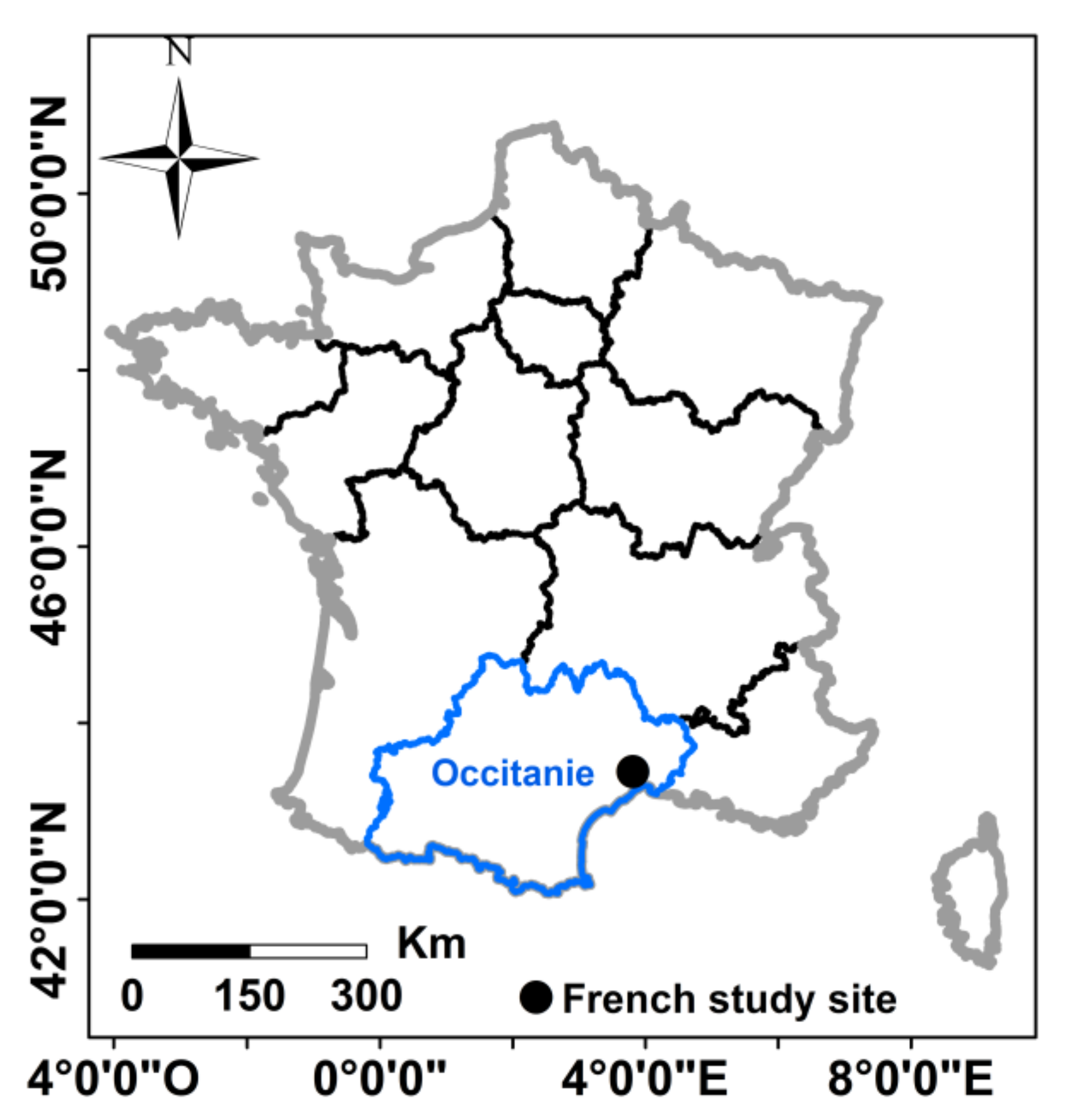
2.1. French Study Site

A study site located in the Occitanie region of France (centered on 3.80°E and 43.67°N, Figure 1) was chosen to validate our approach for the operational mapping of soil moisture. Relatively flat, it is composed mainly of forest, vineyard, grasslands, and agricultural fields (mainly wheat). The climate of the study site is Mediterranean with a rainy season between mid-October and March and an average cumulative rainfall of approximately 750 mm. The average air temperature varies between 2.9 °C and 29.3 °C. The top soil texture of the agricultural fields is a loam. Twenty-three reference plots with areas between 0.6 and 9 ha were selected over our study site, with 10 grasslands and 13 plots of wheat.
Twenty-five SAR images acquired by Sentinel-1 and 11 optical images acquired by Sentinel-2 were used in this study. In addition, in situ campaigns were conducted simultaneously with SAR acquisitions to collect the in situ measurements of soil moisture in our reference plots.

2.1.1. Sentinel-1 Images

The SAR images were obtained from the Sentinel-1A (S1A) and Sentinel-1B (S1B) satellite constellation operating at the C-band (wavelength ~6 cm). Over our study site, S1A and S1B provide images every 6 days. The Sentinel-1 (S1) images are downloadable from the Copernicus website (https://scihub.copernicus.eu/dhus/#/home). The 25 S1 images used were acquired between September 2016 and May 2017 in IW imaging mode with the VV and VH polarizations (this acquisition mode is the primary conflict-free mode for land). In addition, S1 images were generated from the high-resolution Level-1 Ground Range Detected (GRD) product with a spatial resolution of 10 m × 10 m. For all S1 images, the study site is imaged with an incidence angle (θ) of approximately 39°.
The Sentinel-1 Toolbox (S1TBX), developed by the ESA (European Spatial Agency), was used to calibrate the S1 images. The calibration aims to convert the digital number values of S1 images into backscattering coefficients (σ°) in a linear unit. For each reference plot, the mean backscattering coefficient was calculated from each calibrated S1 image by averaging the σ° values of all pixels within that plot. The average of σ° pixels values reduces the speckle noise.

2.1.2. Sentinel-2 Images

Eleven free optical images were obtained from the Sentinel-2A (2A) satellite on dates close to S1 images (less than 2 weeks). The S2A images were downloaded from the Theia (French land data service center) website, the French land data center (https://www.theia-land.fr/). The Theia website provides S2A images that are corrected for atmospheric effects and ortho-rectified [42,43]. Currently, Sentinel-1 (S1) and Sentinel-2 (S2) sensors provide images with revisit time of 6 and 5 days, respectively. In theory, it is possible to obtain one S1 image and one S2 image with difference in time less than one week. If the optical image closest to the radar image is cloudy, the optical image acquired two weeks before or after the radar image acquisition date could be used because in agriculture areas the vegetation does not change a lot within one or two weeks.
First, the NDVI maps were derived from the S2A images. Then, from each calibrated S2A image the NDVI pixel values within each reference plot were averaged to characterize the vegetation condition of that plot. Finally, for each reference plot, to derive the NDVI values for the S1 acquisition dates, a linear interpolation was performed using the NDVI value corresponding to the S2A image acquired before the radar acquisition date and the NDVI value of the S2A image acquired after the radar acquisition date. For our reference plots, the NDVI values ranged between 0.13 (almost bare soil) and 0.92 (vegetation height ~85 cm).

2.1.3. In Situ Measurements

Soil moisture (mv) was measured within a window of 2 h with respect to the S1 acquisition date. For each reference plot, twenty-five to thirty measurements of volumetric soil moisture were conducted in the top 5 cm of soil by means of a calibrated TDR (Time Domain Reflectometry) probe. All soil moisture measurements within each plot were averaged to provide a mean value for each plot. The range of the soil moisture value is between 7.0 and 36.3 vol %.
The soil roughness parameter Hrms (root mean surface height) was not measured. Only information about the roughness class was collected for each reference plot at each field campaign according to three classes: smooth areas (sowing) with a root mean square surface height (Hrms) lower than 1 cm, medium roughness areas (slightly plowed soil) with an Hrms between 1 cm and 2 cm, and rough areas (well plowed soil) with an Hrms higher than 2 cm. These roughness thresholds that are used for each class are obviously approximations, but because of our experience in collecting roughness measurements over the past 20 years, we will assume these are fairly reliable observations.
Finally, our French database is composed of 289 elements with radar backscattering coefficients (in the VV and VH polarizations), NDVI values, and in situ measurements of soil moisture (mv) and roughness class. For a specific SAR acquisition date, each element of the real database represents a reference plot with an associated mean mv value, SAR information (mean incidence angle and mean backscattering coefficients in the VV and VH), and mean NDVI value. Among the 289 database elements, 18 samples represent smooth areas, 259 are medium-rough areas, and 12 are rough areas. This database was only used to validate our inversion approach for soil moisture mapping.

2.2. SAR Signal Sensitivity Analysis

In this section, the sensitivity of SAR signal to soil moisture (mv) in the VV and VH polarizations was analyzed for different NDVI ranges using the Tunisian and French databases together (Figure 2). Figure 2 was created using the French database in addition to the Tunisian database. The results show that for an NDVI between 0.1 and 0.75, the radar signal in both the VV and VH polarizations (incidence angle approximately 39°) increases as soil moisture increases (mv between 5 and 40 vol %). The sensitivity of the radar signal to soil moisture is approximately 0.16 dB/[vol %] for the VV and 0.13 dB/[vol %] for the VH, with an NDVI between 0.1 and 0.75. The decrease in the radar signal sensitivity to soil moisture is observed in Figure 2 when the NDVI increases for the NDVI values between 0 and 0.75. Beyond 0.75 (vegetation height > 70 cm), the radar signal in the VV and VH tends to become saturated for an mv between 5 and 40 vol %. The saturation is related to the high attenuation of the radar signal by the well-developed vegetation cover. Accordingly, only database elements with NDVI values lower than 0.75 will be used to validate our inversion approach for soil moisture estimates because the penetration of the radar signal in the C-band seems very weak for NDVI values higher than 0.75.
The decrease in the radar signal sensitivity to the soil moisture when the vegetation cover increases was reported in the studies of Baghdadi et al. [30] and El Hajj et al. [44]. In Baghdadi et al. [30], the sensitivity of the radar signal at the C-band (VV polarization and high incidence angle) is 0.11 dB/[vol %] and 0.05 dB/[vol %] for a grassland biomass lower and higher than 1 kg/m2, respectively. Moreover, the results showed that the sensitivity of the radar signal in the VV polarization to the soil moisture was higher than that in the VH polarization (0.08 dB/[vol %] and 0.01 dB/[vol %] for a grassland biomass lower and higher than 1 kg/m2, respectively).

3. Soil Moisture Mapping Methodology

Our approach for the operational soil moisture mapping uses the neural networks technique to invert the radar signal. The neural networks (NNs) are trained using a synthetic database of the C-band backscattering coefficients in the VV and VH polarizations (incidence angle “θ” between 20° and 45°), soil moisture (mv), surface roughness (Hrms) and NDVI. The synthetic database is built using a parameterized Water Cloud Model (WCM) [26] combined with the modified Integral Equation Model (IEM) [15,17]. The WCM used was parameterized using a wide range of soil moisture values (between 4.0 and 39.7 vol %), surface roughness (between 0.7 cm and 4.6 cm), and NDVI (between 0.08 and 0.86), all of which were obtained from agricultural fields (mainly cereals). The development of the inversion method consists of five steps:
(1)
Simulate the radar backscattering coefficients in the VV and VH using the parameterized WCM;
(2)
Generate a noisy synthetic SAR C-band database by noising the data simulated by the WCM (step 1) to use the SAR database close to the real SAR data. The NDVI values used as input to the WCM were also noised to better represent the real NDVI values computed from the optical images;
(3)
Divide the synthetic database into two equal sub-databases, one for neural network training and one for neural network validation;
(4)
Train and validate the neural networks using the synthetic training and validation sub-databases, respectively;
(5)
Finally, apply the trained neural networks to the real database (French database) of the SAR and NDVI measurements computed from Sentinel-1 and Sentinel-2 images, respectively, to estimate the soil moisture.
For the proposed approach, neural networks need to be trained on wide database (with soil and vegetation parameters the most encountered in agricultural environments) simulated from calibrated physical model (WCM coupled with the modified IEM). The NNs trained only one time could be next used to derive the soil moisture from S1 and S2 images. As a case study, the developed approach was applied in using the Sentinel-1 and Sentinel-2 images for operationally mapping the soil moisture at high spatial resolution (up to plot scale) over the Occitanie region in France.

3.1. Radar Backscattering Model

In this study, the Water Could Model (WCM) was combined with the modified Integral Equation Model (IEM) and used to simulate the radar response for different conditions of vegetation and soil in an agricultural context. The WCM is the most commonly used model to estimate soil moisture in the presence of vegetation cover because it uses a simple formulation and consequently, it could be easily inverted [21,29,31,32,33,45,46,47,48]. In the WCM, the total backscattered signal is equal to the sum of vegetation contribution and soil contribution attenuated by the vegetation layer. The soil contribution is a function of the soil moisture and roughness. The vegetation contribution and the attenuation are computed using one or more vegetation parameters, such as the leaf area index, NDVI, and vegetation water content [25,26,27,29,30,49,50].
The parametrization of the WCM used in this work was performed in a previous study [26] for the VV and VH polarizations (θ between 18° and 40°) in using wide database of SAR C-band measurements, NDVI values derived from optical images, and in situ measurements of soil moisture (mv) and soil roughness (Hrms). In Baghdadi et al. [26], the WCM was parameterized in using data collected over a study site located in central Tunisia (Kairouan Plain: 35°1’−35°55’ N-9°23’−10°17’ E) that contains mainly agricultural fields of cereals. The NDVI values ranged between 0.1 and 0.86, the mv values were between 4.0 and 39.6 vol %, and the Hrms was between 0.7 cm and 4.6 cm. The vegetation contribution and the vegetation attenuation effects were computed using the NDVI as the vegetation descriptor. In addition, the soil contribution was simulated using the IEM modified by Baghdadi et al. [15,17]. The results showed that the parameterized WCM simulates the backscattering coefficients in the VV and VH polarizations with an accuracy (Root Mean Square Error “RMSE”) of approximately 1.4 dB (R2 approximately 0.60), which is close to the S1 measurement accuracy [51,52].

3.2. Synthetic Database

The parameterized WCM was used to generate a synthetic database of backscattering coefficients in the VV and VH (σ°VV and σ°VH) from a wide range of θ (20° to 45°), mv (2 to 40 vol %), Hrms (0.5 to 3.8 cm), and NDVI (0 to 0.75) values. Each element of the database is composed of a combination of four input parameters θ, mv, Hrms, NDVI and a simulated σ°VV and σ°VH. The synthetic database comprises 84240 elements (Table 1).
To make the synthetic database of backscattering coefficients more realistic (i.e., similar to real SAR data), the error corresponding to Sentinel-1 radiometric accuracy was added to the simulated backscattering coefficients. This error is approximately 0.70 dB (3σ) for the VV polarization and 1.0 dB (3σ) for the VH polarization [52]. Thus, we considered two absolute zero-mean Gaussian random additive noises with a standard deviation of ±0.7 and ±1.0 dB to be added to the simulated backscattering coefficients in the VV and VH, respectively. Moreover, given that the relative error in the NDVI derived from the optical images is approximately 15% at the most [53,54], the NDVI values in the synthetic database were noisy, with a zero-mean Gaussian additive relative noise of 15%.
For each synthetic database backscattering coefficient, 10 random noises were used (zero-mean Gaussian noise with a standard deviation of 0.7 and 1.0 dB for the VV and VH, respectively). In addition, for each NDVI in the synthetic database, 10 random noises were also used. The synthetic database with noisy backscattering coefficients and NDVI is called the noisy synthetic database in this paper. It is composed of 8,424,000 elements. Finally, the noisy synthetic database was randomly divided into two equal sub-databases, one for the neural network training (noisy training database) and one for the neural network validation (noisy validation database).

3.3. Artificial Neural Networks (ANN)

In this study, the neural network technique was used to invert the SAR data for estimating the soil moisture because the direct inversion of the IEM model is not possible. Three SAR configurations for estimating the soil moisture are considered:
  • Configuration 1: incidence angle, noisy radar signal at VV polarization, and noisy NDVI are the inputs of the network;
  • Configuration 2: incidence angle, noisy radar signal at VH polarization, and noisy NDVI are the inputs of the network; and
  • Configuration 3: incidence angle, both noisy radar signal at VV and VH polarizations and noisy NDVI are the inputs of the network.
Neural networks (NNs) were trained in using the noisy synthetic training database generated from the parameterized WCM and the modified IEM. The Hrms was not used as an input parameter for the neural networks training and validation. Although, synthetic database was simulated using Hrms values between 0.5 and 3.8 cm.
All neural networks were trained in using the Levenberg-Marquardt algorithm [55] with two hidden layers [20]. The number of neurons for each hidden layer is 20 [20,56]. Linear and tangent-sigmoid transfer functions were associated with the first and second hidden layers, respectively.
To improve the soil moisture estimates, a priori knowledge about the soil moisture state is introduced. Indeed, it is easily to define from the weather forecasts (precipitation and temperature) if the soil is either dry to slightly wet (no precipitation for many days before SAR acquisition) or very wet (heavy rainfall preceding SAR acquisition) [20]. The integration of a priori information constrains the range of possible soil moisture parameter values estimated by the neural networks and thus leads to a better estimation of the soil moisture. The requirement for rainfall information is not an obstacle for our operational approach to soil moisture mapping at a high spatial resolution because the information about rainfall (date and amount) are easily available from the in situ sensors. In the case of soil moisture mapping at a low spatial resolution, rainfall remote sensing satellite products (such as the Tropical Rainfall Measuring Mission: TRMM) could be used to define a priori knowledge about the soil moisture. Accordingly, neural networks are built either using or neglecting a priori information on the soil moisture conditions:
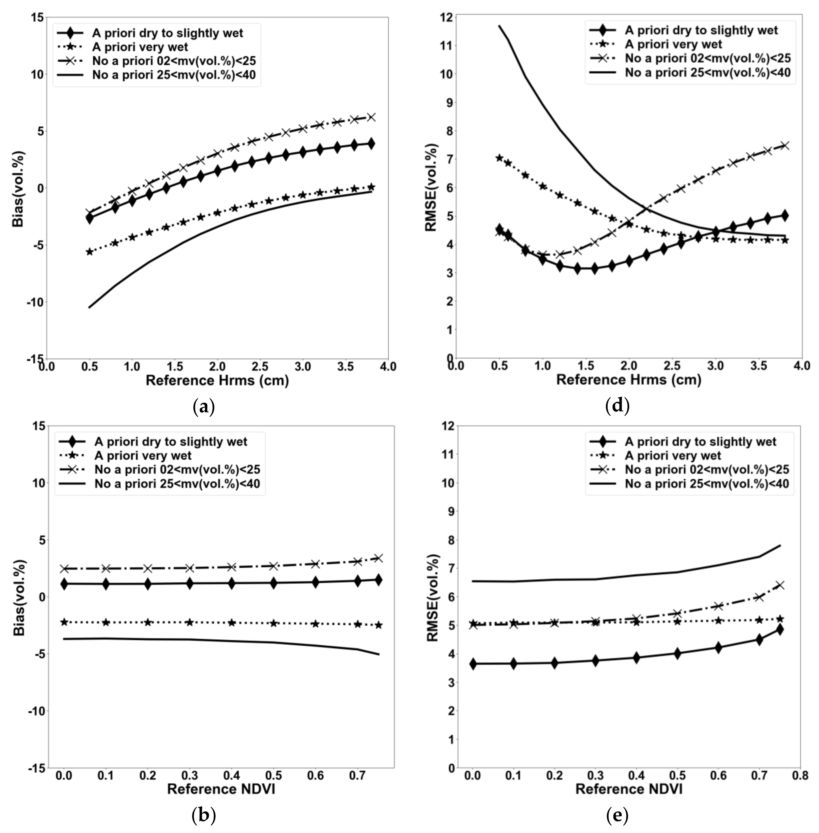
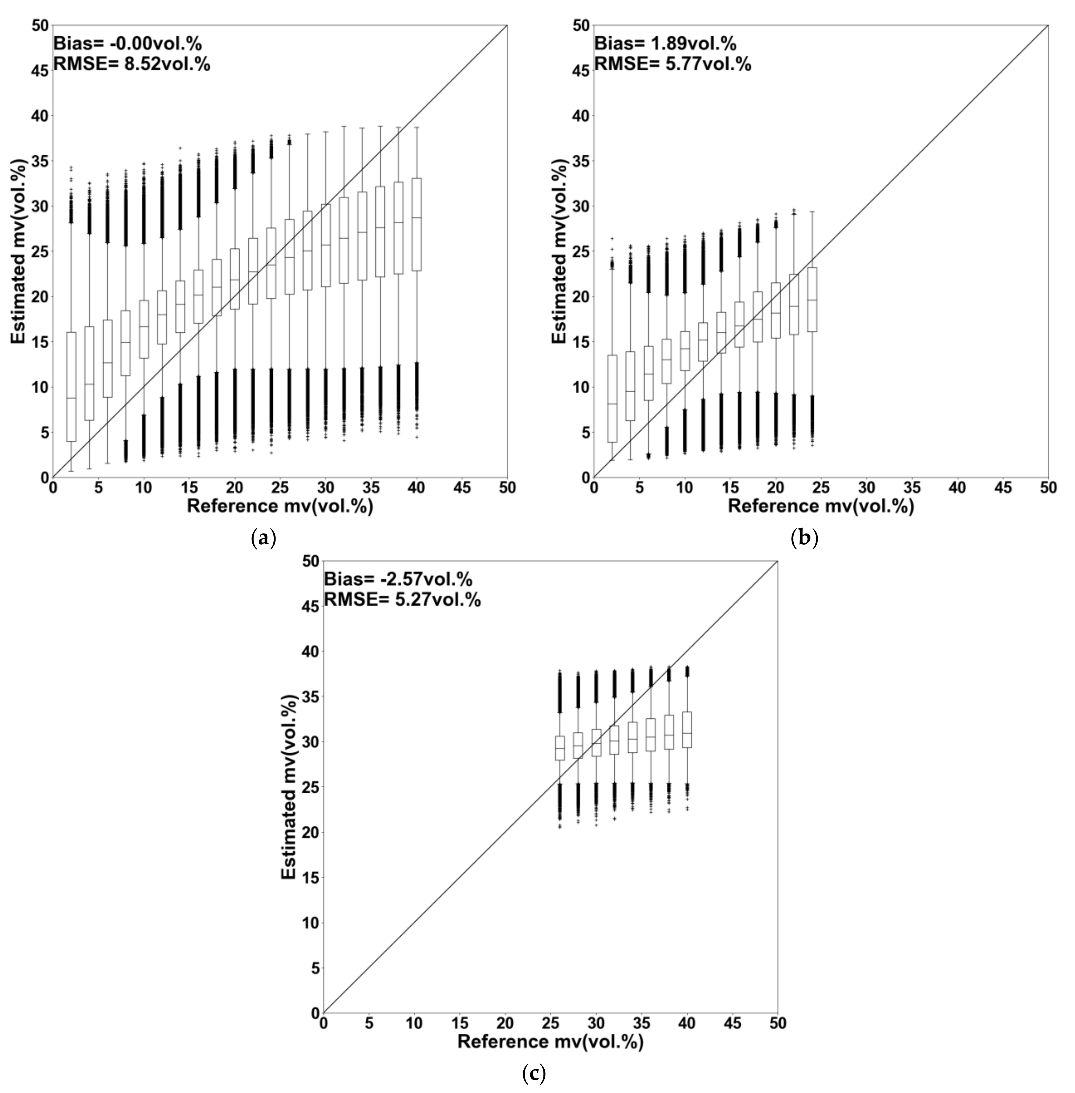
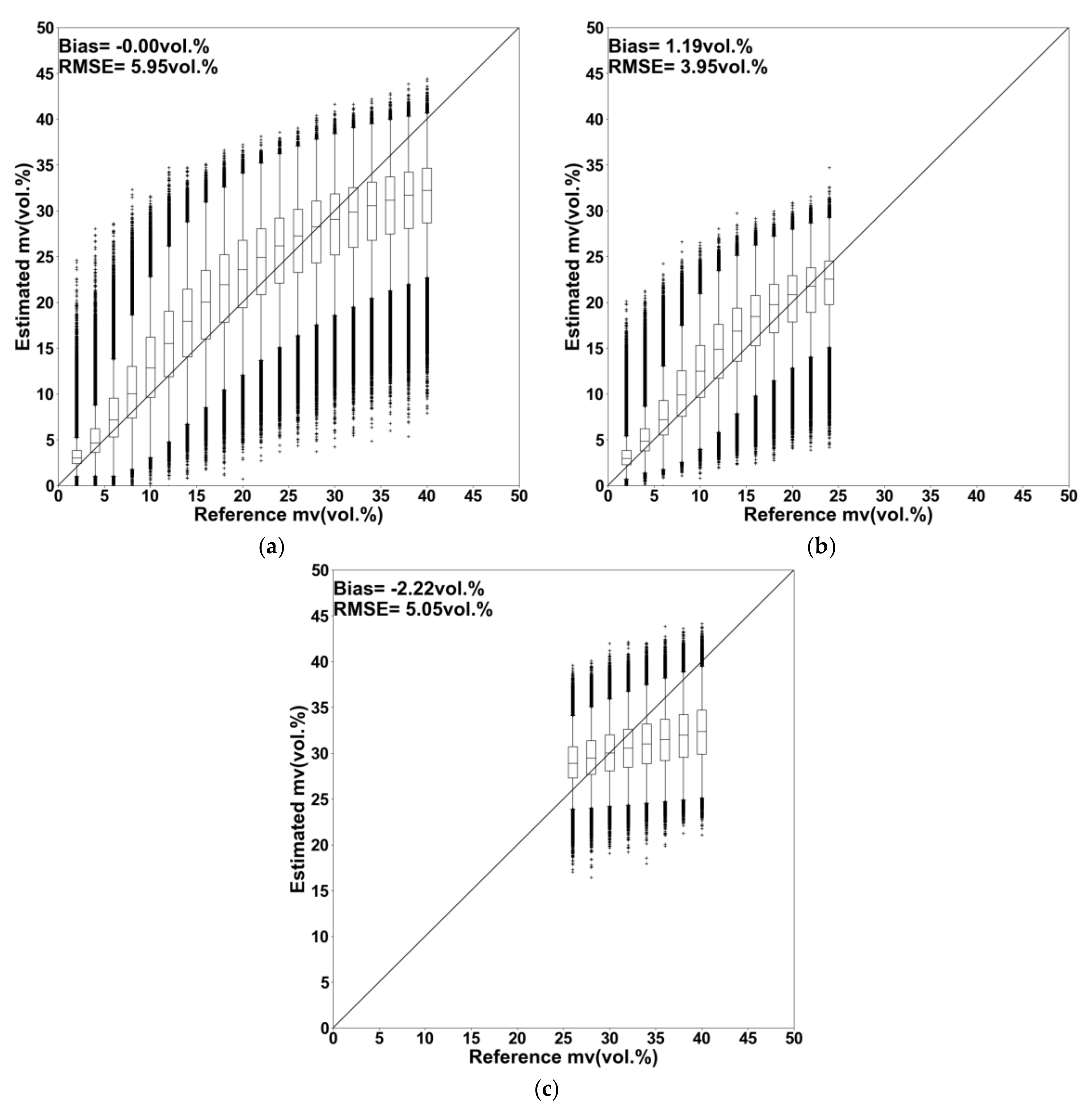
  • Case 1: No a priori information is available for the soil moisture state. In this case, the mv will be estimated between 2 and 40 vol %.
  • Case 2: A priori information is available for mv. The soil is supposed to be dry to slightly wet according to expertise based mainly on meteorological data (precipitation, temperature). Soil moisture values are assumed to range from 2 to 25 vol %.
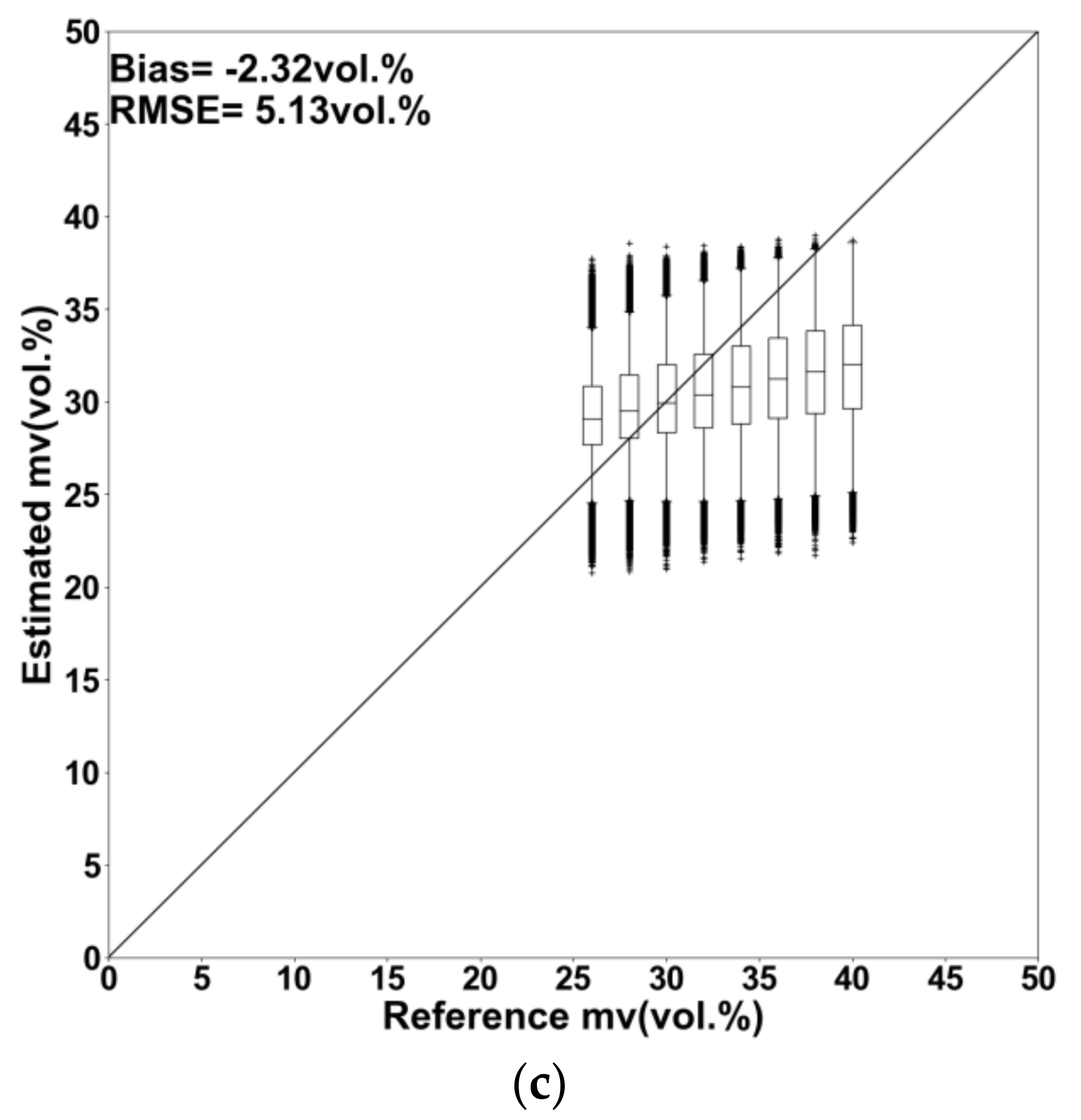
  • Case 3: A priori information is available for mv. The soil is supposed to be very wet according to the expertise of the meteorological data. The mv values are assumed to vary between 25 and 40 vol %.
For the case with no a priori information (case 1), the three neural networks (configurations 1, 2, and 3) were developed using the entire training database (mv between 2 and 40 vol %). For the two cases with a priori information on the mv (cases 2 and 3), an overlap of 10 vol % on the mv is considered between the databases used for the training of the networks. For a priori information that soil is dry to slightly wet (case 2), the three neural networks (configurations 1, 2, and 3) were developed using the training database elements with the mv between 2 and 30 vol %. For a priori information that soil is very wet (case 3), the three neural networks (configurations 1, 2, and 3) were developed using the training database elements with the mv between 20 and 40 vol %. To summarize, 9 neural networks are developed for the estimation of soil moisture. Table 2 shows the mains properties for each neural network.
This approach, which uses a priori information on the soil moisture, is relevant even when the agricultural plots in the study area are irrigated. If the SAR images are acquired during the dry season with irrigation activities occurring at the study site, the use of a priori information on the mv (dry to slightly wet soils) could lead to an underestimation of the mv if the real soil moisture is higher than 30 vol %.
First, the analysis of the performance of neural networks is carried out using the noisy validation database for each case (no a priori information, a priori information for dry to slightly wet soils, and a priori information for very wet soils). The estimated mv from the neural networks is compared to the reference mv and the errors for the mv estimates were quantified by means of the bias (Estimated mv – Reference mv) and the Root Mean Square Error (RMSE). In addition, the error for the mv estimates (RMSE and Bias) was analyzed according to the NDVI, Hrms, and θ values.
Finally, the nine developed neural networks are used to invert real SAR data. The inversion was performed using real SAR data as well as the NDVI values (calculated from the optical images) instead of the noisy backscattering coefficients and NDVI values.

4. Results

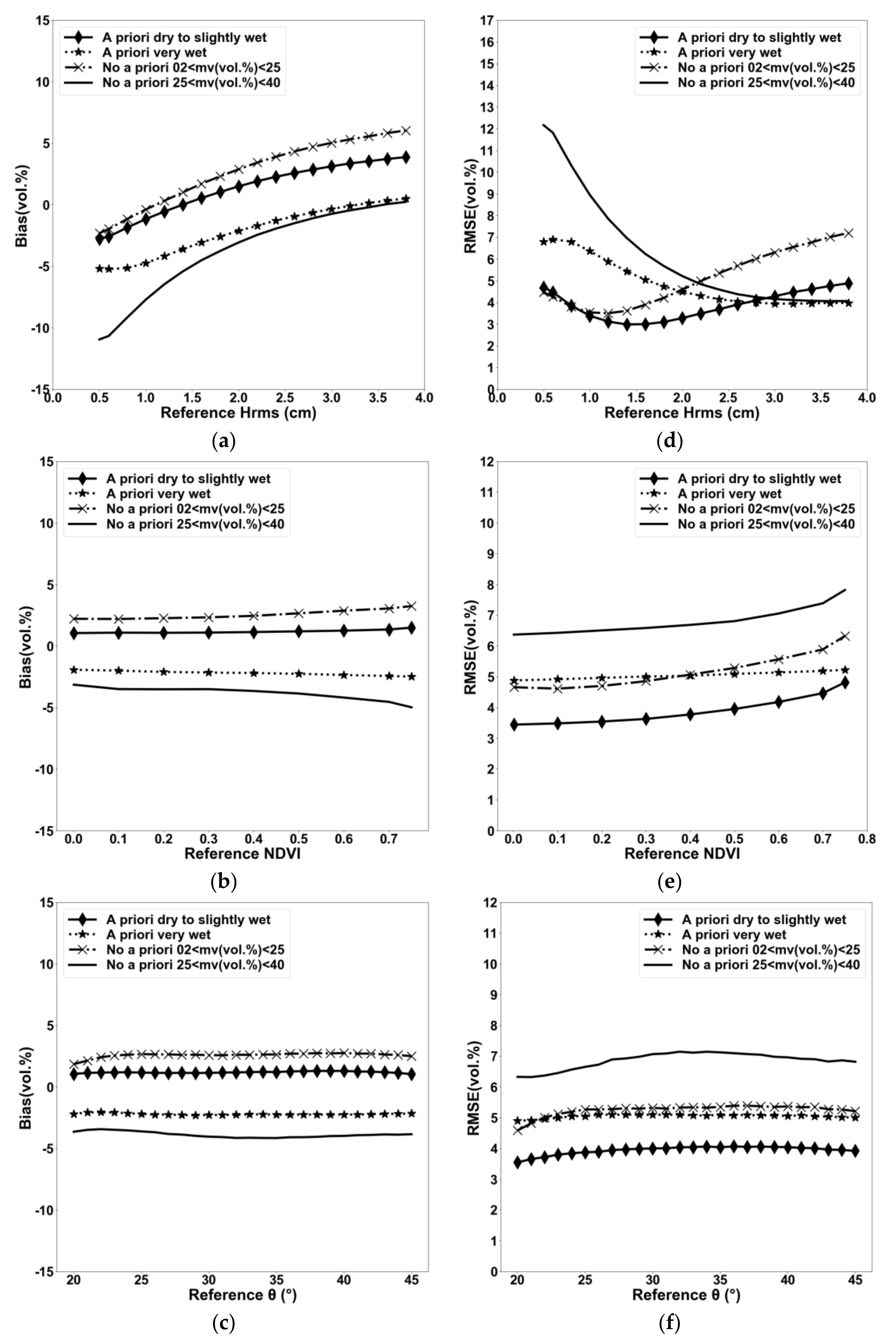
4.1. Using the Synthetic Database

Given that the best results were obtained using the VV alone (NN1, NN1_dry, and NN1_wet), the results from NN1, NN1_dry, and NN1_wet will be thoroughly commented upon (Section 4.1.1). On the other hand, the results obtained with the VH alone (NN_2, NN_2_dry, and NN_2_wet), as well as the VV and VH together (NN_3, NN_3_dry, and NN_3_wet), will be briefly discussed (Section 4.1.2 and Section 4.1.3).

4.1.1. Neural Networks Using the VV Alone (NN1, NN1_dry, and NN1_wet)

Figure 3 shows the performance of the neural networks that take σ°VV, θ, and NDVI as input parameters. For NN1 (no a priori information on the mv), the training and validation were performed using all training and validation database elements, respectively (mv between 2 and 40 vol %). NN1_dry was trained using the noisy training database elements with mv between 2 and 30 vol % and next was validated using the noisy validation database elements with mv between 2 and 25 vol %. For NN1_wet, the training was performed using the noisy training database elements with mv between 20 and 40 vol %, and the validation was realized using the noisy validation database elements the mv between 25 and 40 vol %.
The neural network built without the use of a priori information on the mv (NN1) shows a non-biased estimation of mv and an RMSE of 6.1 vol % (Figure 3a). Moreover, errors on the mv estimated from NN1 was analyzed for a reference mv lower and higher than 25 vol %. For a reference mv lower than 25 vol %, the results show that NN1 yielded an overestimation of the reference mv of 2.7 vol % and an RMSE equal to 5.5 vol %. For a reference mv higher than 25 vol %, an underestimation of mv (bias = −4.1 vol %) and an RMSE equal to 6.9 vol % were obtained with NN1.
For a reference mv lower and higher than 25 vol %, the accuracy of mv estimates (bias and RMSE) is improved with the consideration of a priori information on the mv (dry to slightly wet soil conditions “NN1_dry” and very wet “NN1_wet”) (Figure 3b,c). Indeed, for a reference mv lower than 25 vol %, the use of NN1_dry yields a smaller bias “estimated mv—reference mv” (1.2 vol %) and an RMSE (4.0 vol %) in comparison to NN1 (no a priori information on the mv) (Figure 3b). Similarly, for a reference mv between 25 and 40 vol %, the use of NN1_wet improves the bias by 1.8 vol % (bias = −2.3 vol %) and the RMSE by 1.8 vol % (RMSE = 5.1 vol %) (Figure 3c).
Furthermore, the evolution of errors (bias and RMSE) on the mv estimated from the NN1, NN1_dry, and NN1_wet are analyzed according to the Hrms, NDVI, and θ (Figure 4). In general, the results show that the bias varies with the Hrms and remains constant with the NDVI and θ. In the case of no a priori information on the mv (NN1) and for a reference mv between 2 and 25 vol % (Figure 4a), the bias varies from −2.2 vol % to 6.2 vol % as the Hrms increases from 0.5 to 3.8 cm (underestimation for an Hrms lower than 1.2 cm and overestimation for an Hrms higher than 1.2 cm). However, the bias remains constant (approximately 2.7 vol %) with the NDVI for NDVI between 0 and 0.75 and with θ for θ between 20° and 45° (Figure 4b,c). In the case of no a priori information (NN1), and for a reference mv between 25 and 40 vol %, the mv estimates are highly underestimated for an Hrms equal to 0.5 cm (bias = −10.5 vol %). This underestimation decreases when the Hrms increases to reach approximately 0.3 vol % for an Hrms = 3.8 cm (Figure 4a). Figure 4b,c show that the difference between the estimated and reference mv is approximately −4.1 vol % regardless of the NDVI and θ values in the case of NN1 and for very wet soil conditions.
The use of a priori information on the mv (dry to slightly wet “NN1_dry” and very wet “NN1_wet”) yields a similar bias behavior according to the Hrms, NDVI and θ, as in the case of no a priori information (Figure 4). However, the bias level is lower with NN1_dry and NN1_wet than with NN1. Using a priori information on the mv with dry to slightly wet soil conditions, NN1_dry slightly improves the bias for an Hrms lower than 1.4 cm (less than 1 vol %), whereas the improvement varies from 1.1 vol % for an Hrms equal to 1.4 cm to 2.3 vol %, for an Hrms equal to 3.8 cm (Figure 4a).The use of a priori information with very wet soil conditions (NN1_wet) improves the bias significantly for an Hrms lower than 2 cm (improvement decreases from 4.9 to 1.2 as the Hrms increases from 0.5 to 2 cm) and slightly improves the bias for an Hrms higher than 2 cm (improvement is less than 1 vol %) (Figure 4a). In using NN1_dry, the bias by approximately 1.5 vol % for all NDVI and θ values (Figure 4b,c). In using NN1_wet, the improvement in the bias varies between 1.5 vol % for an NDVI = 0 to 2.6 vol % for an NDVI = 0.75 (Figure 4b), and it is approximately 1.8 vol % for all θ values (Figure 4c).
The analysis of the RMSE on the mv estimates in the case of no a priori information on the mv (NN1) with a reference mv between 2 and 25 vol % shows that the RMSE decreases slightly from 4.4 vol % to 3.6 vol % when the Hrms increases from 0.5 to 1.2 cm. Beyond 1.2 cm, the RMSE increases greatly from 3.6 to 7.5 when the Hrms increases from 1.2 to 3.8 cm (Figure 4d). Moreover, the results show that the RMSE increases slightly from 5.0 to 6.4 vol % when the NDVI increases from 0 until 0.75 (Figure 4e). The RMSE seems not depends on θ with an RMSE on the mv of approximately 5.5 vol % for a θ between 20 and 45° (Figure 4f). In the case of no a priori information on the mv with a reference mv between 25 and 40 vol %, the RMSE on the mv decreases from 11.7 vol % to 4.3 vol % when the Hrms increases from 0.5 to 3.8 cm (Figure 4d). Moreover, the results show that the RMSE has a slight increase of approximately 1.3 vol % (from 6.5 to 7.8 vol %) when the NDVI increases from 0 to 0.75 (Figure 4e). Finally, the RMSE increases slightly from 6.2 to 6.9 vol % for θ between 20 and 45° (Figure 4f).
In the case of a priori information on the mv with dry to slightly wet soil conditions, NN1_dry improves the RMSE (calculated using the validation database with the mv between 2 and 25 vol %) by less than 1 vol % for an Hrms less than 1.6 cm, by 1.6 vol % for an Hrms between 1.6 and 2.8 cm, and by approximately 2.3 vol % for an Hrms higher than 2.8 cm (Figure 4d). In addition, the RMSE on the mv estimates is improved by approximately 1.5 vol % for an NDVI between 0 and 0.75 and for θ between 20° and 45° when using NN1_dry, compared to the results obtained with NN1 (Figure 4e,f). The use of a priori information on the mv with very wet soil conditions (NN1_wet) improves the RMSE on the mv estimates (calculated using the validation database with an mv between 25 and 40 vol %). This improvement is significant for a low Hrms (4.6 vol% for Hrms = 0.5 cm) and decreases when the Hrms increases (0.2 vol % for Hrms = 3.8 cm) (Figure 4d). In comparison to NN1, the network NN1_wet improves the RMSE from 1.5 vol % for an NDVI = 0 to 2.6 vol % for an NDVI = 0.75 (Figure 4e). In addition, Figure 4f shows that the decrease of the RMSE on the mv estimates is in the same order (approximately 1.8 vol %) for all θ between 20° and 45° (RMSE = 6.9 vol % with NN1 and RMSE = 5.1 vol % with NN1_wet).

4.1.2. Neural Networks Using the VH Alone (NN2, NN2_dry, and NN2_wet)

Figure 5 shows the performance of the VH polarization (inputs: noisy σ°VH, θ, and noisy NDVI) for estimating soil moisture. The neural network built with no a priori information on the mv (NN2) shows a non-biased estimation of mv and an RMSE of 8.5 vol % (Figure 5a). Moreover, for a reference mv lower than 25 vol %, the results show that NN2 provides an overestimation of the reference mv of 4.6 vol % with an RMSE of 7.6 vol %. For a reference mv higher than 25 vol %, the mv estimated from NN2 underestimates the reference mv by 6.9 vol % with an RMSE equal to 9.7 vol %. Moreover, the results show that the use of both a priori information for dry to slightly wet (NN2_dry) and very wet soil conditions (NN2_wet) allows more precise soil moisture estimates. For a reference mv between 2 and 25 vol %, the RMSE on the mv estimates decreases from 7.6 vol % with NN2 to 5.8 vol % with NN2_dry (bias decreases from 4.6 vol % with NN2 to 1.9 vol % with NN2_dry) (Figure 5a,b). In very wet soil conditions, the use of a priori information improves the RMSE on the mv estimates from 9.7 vol % with NN2 to 5.3 vol % with NN2_wet (bias decreases from −6.9 vol % with NN2 to −2.6 vol % with NN2_wet) (Figure 5a,c).
In the case of no a priori information, the errors on the mv estimated from the VH (NN2) are higher than those from the VV (NN1) for both soil conditions, dry to slightly wet soils and very wet soils (Figure 3a and Figure 5a). For an mv between 2 and 25 vol %, the RMSE on the mv estimates are 7.6 vol % with NN2 (bias = 4.6 vol %) and 5.5 vol % with NN1 (bias = 2.7 vol %). For an mv between 25 and 40 vol %, the RMSE on the mv estimates are 9.7 vol % with NN2 (bias = −6.9 vol %) and of 6.9 vol % with NN1 (bias = −4.1 vol %). Similarly, the use of a priori information in the case of dry to slightly wet soils (reference mv between 2 and 25 vol %), the errors are higher with the VH (bias = 1.9 vol %, RMSE = 5.8 vol %) than with the VV (bias = 1.2 vol %, RMSE = 4.04 vol %) (Figure 3b and Figure 5b). Finally, in the case of a priori information on the mv with very wet soils (reference mv between 25 and 40 vol %), the errors on the mv estimated from the VH alone (bias = −2.6 vol % and RMSE = 5.3 vol %) and the VV alone (bias = −2.3 vol %, RMSE = 5.1 vol %) are similar (Figure 3c and Figure 5c).
The behavior of errors (bias and RMSE) on the mv estimates with the VH polarization (NN2, NN2_dry, and NN2_wet) according to the Hrms, NDVI, and θ is similar to that on the mv estimates with the VV polarization (NN1, NN1_dry, and NN_wet) (Figure 4 and Figure 6). For an mv between 2 and 25 vol % (with or without a priori information on the mv), the RMSE on the mv estimates increases more strongly with the NDVI for the VH alone (NN2, and NN2_dry) than for the VV alone (NN1, and NN1_dry). Indeed, the RMSE increases from 4.1 to 7.3 vol % with NN2_dry and from 3.6 vol % to 4.9 vol % as the NDVI increases from 0 to 0.75 (Figure 4e and Figure 6e). Similarly, in the case of very wet soils without the use of a priori information on the mv, the increase of the RMSE according to the NDVI is more rapid when the VH is used alone instead of the VV alone (Figure 4e and Figure 6e). Finally, with the consideration of a priori information on the mv in the case of very wet soils, the RMSE on the mv estimated from the VV alone and the VH alone do not depend on the NDVI (RMSE approximately 5.1 vol %) (Figure 4e and Figure 6e).

4.1.3. Neural Networks Using the VV and VH Together (NN3, NN3_dry, and NN3_wet)

The use of the VV and VH polarizations together as inputs in the neural networks (NN3, NN3_dry, and NN3_wet) to estimate soil moisture provides an accuracy similar to that obtained with the use of VV alone (NN1, NN1_dry, and NN1_wet). As observed in the case of VV alone, the use of both VV and VH with consideration of a priori information reduces the errors on the mv estimates (Figure 7). As an example, for a reference mv between 2 and 25 vol %, a bias of 1.2 vol % and an RMSE of 4.0 vol % are obtained with consideration of a priori information on the mv in the case of dry to slightly wet soil conditions (NN3_dry), compared to a bias of 2.6 vol % and an RMSE of 5.25 vol % with no consideration of a priori information on the mv (NN3) (Figure 7a,b). Moreover, using both VV and VH, the behavior of errors (bias and RMSE) according to the Hrms, NDVI and θ, as well as the values of these errors for each of the Hrms, NDVI and θ values, are approximately the same when the VV polarization is used alone (Figure 4 and Figure 8).

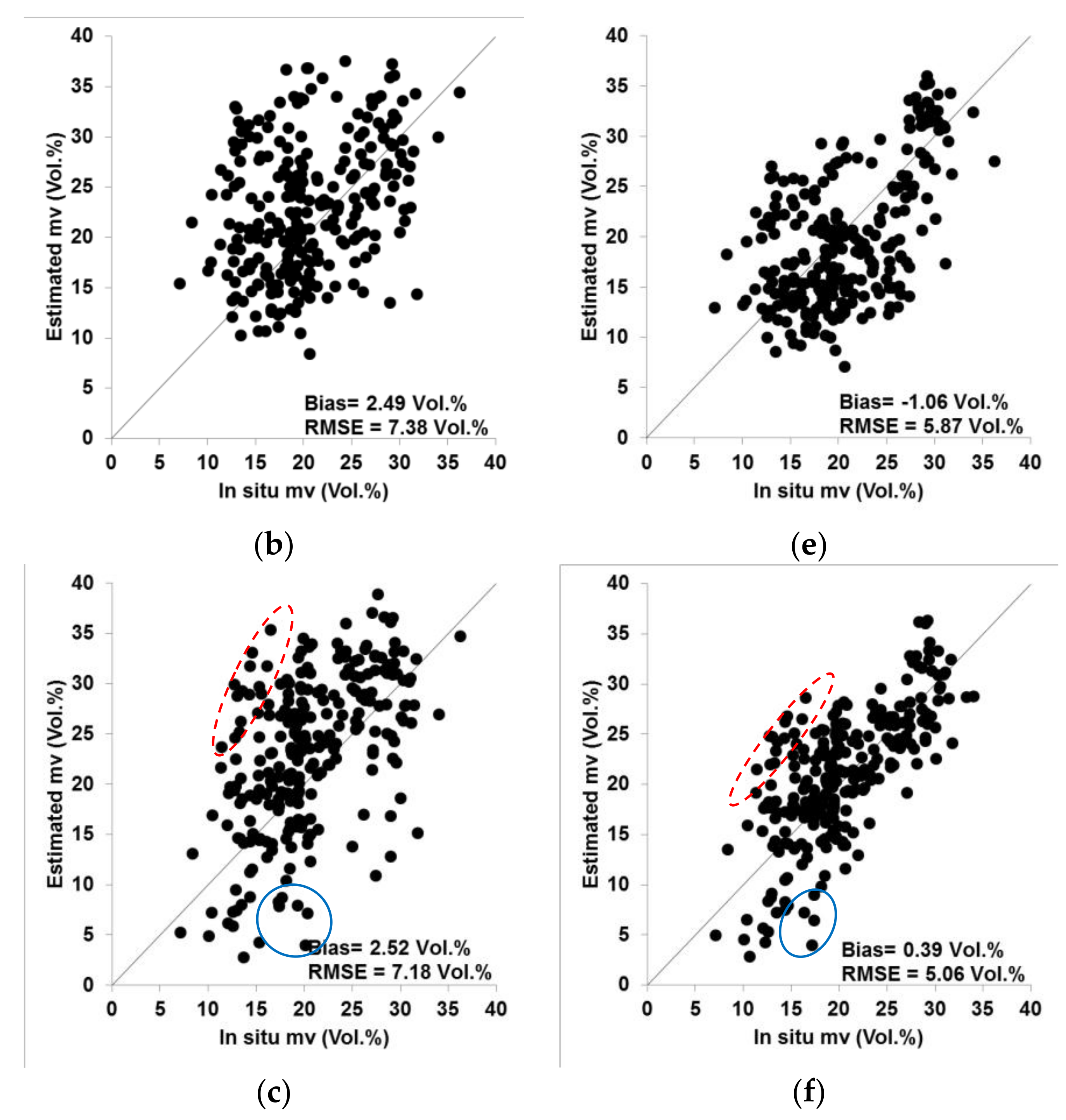
4.2. Using the Real Database

The potential of all developed neural networks (NN1, NN1_dry, NN1_wet, NN2, NN2_dry, NN2_wet, NN3, NN3_dry, and NN3_wet) to estimate soil moisture was evaluated using the real database collected over the French study area. This evaluation was performed using only the database elements with NDVI values lower than 0.75. Indeed, in this study, the results showed that the radar signal in the VV and VH polarizations is not sensitive to soil moisture for an NDVI higher than 0.75. The rain information registered over the study area was used to determine the appropriate neural networks with a priori information. The neural networks with a priori information of dry to slightly wet (NN1_dry, NN2_dry, NN3_dry) were applied if the SAR image was acquired far from a rainy episode or in the context of the fast drying out of soil (high temperatures). The neural networks with a priori information of very wet (NN1_wet, NN2_wet, NN3_wet) were applied if the SAR image was acquired after an intense rainy episode.
Similar results are obtained with the VV alone, the VH alone or using the VV and VH together in the case where no a priori information on the mv is considered with a bias of approximately 2.6 vol % (overestimation of mv) and an RMSE of approximately 7.2 vol %. For all neural networks, the results show that the use of a priori information considerably improves the precision of the estimated soil moisture by approximately 2 vol % for both the bias and RMSE. As an example, the NN1 (no a priori information, VV) overestimates the in situ soil moisture by 2.6 vol % and allows for soil moisture estimates with an accuracy of 7.2 vol % (RMSE), whereas the NN1_dry and NN1_wet (with a priori information, VV) provide a higher accuracy on the estimated mv (bias = 0.2 vol % and RMSE = 5.0 vol %) (Figure 9a,d). Moreover, with the consideration of a priori information on the mv, the results show that the use of the VV alone allows for better soil moisture estimates than the use of the VH alone and a similar precision when both the VV and VH polarization are used. The RMSE on the mv estimates using a priori information on the mv is 5.0 vol % with VV (bias = 0.2 vol %), 5.9 vol % with the VH alone (bias = −1.1 vol %), and 5.1 vol % with the VV and VH together (bias = 0.4 vol %).
For very rough plots with an Hrms higher than 3 cm (red ellipses in Figure 9), the NNs highly overestimate the in situ mv. For example, with the VV alone using a priori information on the mv (NN1_dry and NN1_wet), the estimated mv values are higher than the reference mv by approximately 9 vol %. For very smooth plots with an Hrms lower than 1 cm (blue ellipses in Figure 9), the NNs highly underestimate the in situ mv. For example, using the VV alone with a priori information on the mv (NN1_dry, and NN1_wet), the estimated mv values are lower than the in situ mv by approximately 10 vol %.

5. Discussion

Three inversion configurations using VV alone, VH alone, and both VV and VH were developed. Each inversion configuration was built with and without the consideration of a priori information on the soil moisture condition. The consideration of a priori information (dry to slightly wet and very wet) was realized by limiting the range of soil moisture values in the training database to mv between 2 and 30 vol % for dry to slightly wet soil conditions and between 20 and 40 vol % for very wet soil conditions. These two soil moisture conditions will be selected in an operational procedure of soil moisture estimation according to meteorological information (rainfall events for example).
The developed neural networks were trained using the synthetic database and validated using both real and synthetic databases. Using the synthetic database, the results showed that the consideration of a priori information improves the precision on the soil moisture estimates. In addition, the results showed that the use of VV alone gives a better precision on the soil moisture estimates than using VH alone. Similar precisions were obtained with VV alone and in using VV and VH together. Thus, for soil moisture estimation, it is better to use either VV polarization alone or both VV and VH polarizations with a priori information that could be easily defined from in situ precipitation stations.
For all neural networks, the errors (bias and RMSE) on the mv estimates are found to depend on the Hrms values. For an mv between 2 and 25 vol % (with or without a priori information on the mv), underestimation and overestimation of estimated mv were observed respectively for an Hrms lower and higher than a given threshold of the Hrms. With the consideration of a priori information on the mv in the case of dry to slightly wet soils, this Hrms threshold is equal to 1.5 cm when used the VV alone (NN1_dry) or the VV and VH together (NN3_dry). It is approximately 1 cm when VH is used alone (NN2_dry). In addition, the results show that the RMSE on the mv is the lowest for Hrms between 1 and 2 cm for all SAR inversion configurations (VV alone, VH alone, VV and VH together) used in this study, considering a priori information on the mv in the case of dry to slightly wet soils. In the case of very wet soil conditions (mv between 25 and 40 vol %), an underestimation of mv is observed for all Hrms between 0.5 and 3.8 cm. This underestimation decreased with the increase of soil roughness. In addition, the RMSE on the mv decreases with the Hrms. The lowest RMSE values correspond to Hrms values that are higher than 2.5 cm.
The above conclusions on the dependence between the error on the mv estimates and the Hrms is related to the fact that a smooth surface (Hrms lower than 1 cm) leads to a specular reflection of the emitted radar signal and therefore a low backscatter coefficient, providing an underestimation of the mv with a high RMSE (for all mv values). On the other hand, increasing surface roughness (Hrms higher than 2 cm) results in an increase of the radar backscattering signal that leads to an overestimation of the mv values associated with a high RMSE for dry to slightly wet soils, and provides a slight underestimation with a low RMSE for very wet soils (between 25 and 40 vol %).
Moreover, for a reference mv between 2 and 25 vol % (with or without a priori information on the mv), the increase of errors on the mv estimates according to the NDVI is more rapid for VH alone than for VV alone or for VV and VH together. As VH is more sensitive to vegetation cover, well-developed vegetation cover degrades the precision on the mv estimates when VH is used instead of VV. In the case of very wet soil conditions with a priori information on the mv (reference mv between 25 and 40 vol %), the RMSE on the estimated mv does not depends on the NDVI for all SAR inversion configurations.
From the real database, the results showed that the use of VV alone or VV and VH together, both with the consideration of a priori information on the mv, provides a better precision on the soil moisture estimates (bias approximately 0.2 vol % and RMSE approximately 5.0 vol %). Moreover, the results show that the estimated mv highly overestimates the measured in situ soil moisture (reach 9 vol %) in the case of very rough plots (Hrms > 3 cm). Finally, for very smooth plots (Hrms < 1 cm), the NNs underestimates mv (reach 10 vol %). Thus, the soil moisture estimates will be provided with good accuracy (RMSE approximately 5 vol %) for an Hrms between 1 and 3 cm, while for an Hrms lower than 1 cm and higher than 3 cm, the algorithm tends to underestimate and overestimates the ground-truth mv values by approximately 10 vol %, respectively.
All available SAR data (X, C and L bands) allow estimating the soil moisture in the top 5–10 cm of soil, while crop models need usually soil moisture in soil layer deeper than 10 cm. However; soil moisture in the root zone could be derived from surface soil moisture through a model of water infiltration into the soil [57,58,59,60,61,62,63].

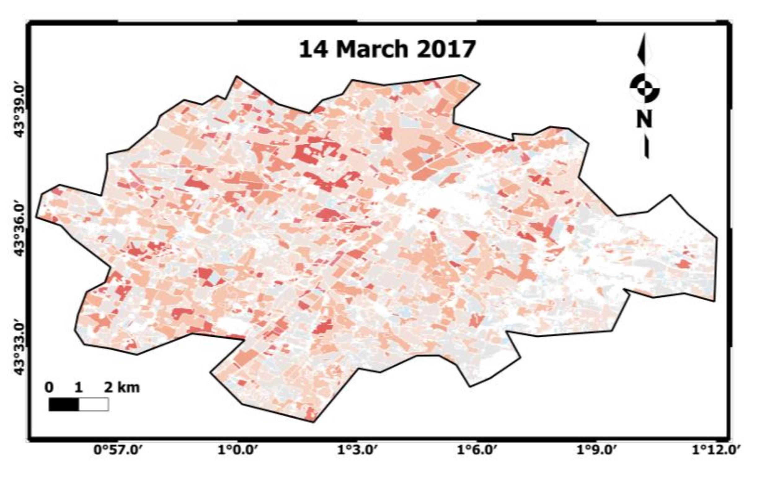
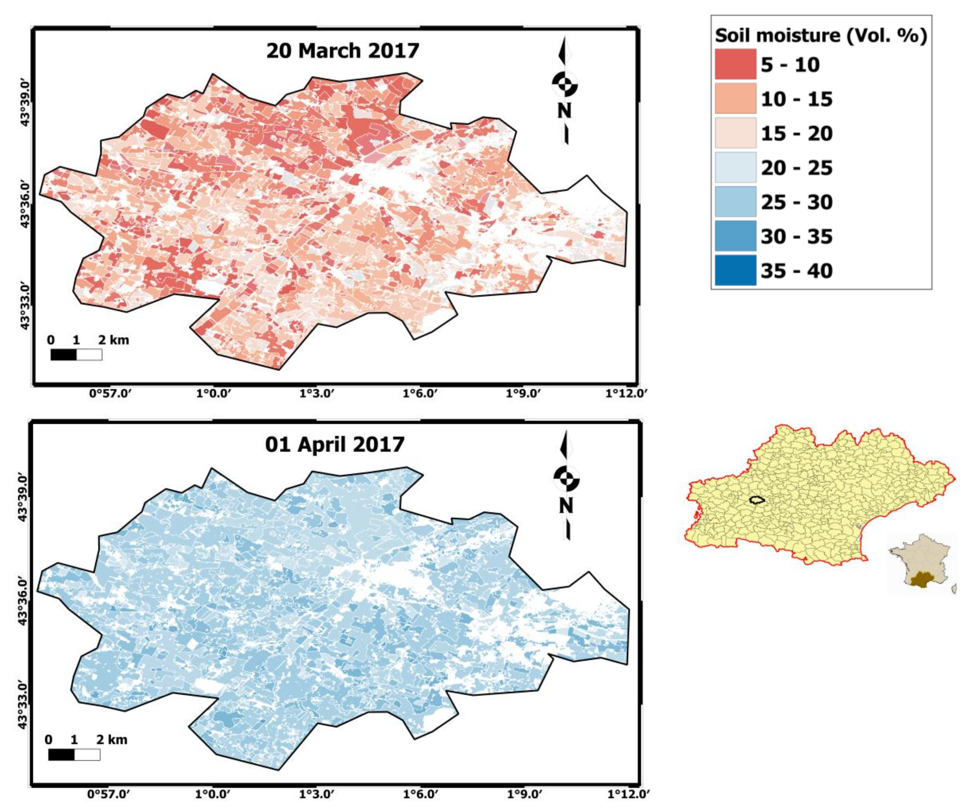
6. Toward Operational Soil Moisture Mapping over Agricultural Areas

From the perspective of operational soil moisture mapping, an operational approach for the estimation of soil moisture is developed in this study. This approach is based on the synergic use of the new free and open accesses radar (Sentinel-1) and optical (Sentinel-2) sensors. The developed methodology was applied for soil surface mapping over the French Occitanie region (area of 72724 km²) located in southern France. The Occitanie region is totally covered by four S1A image footprints and five S1B image footprints. The objective is to operationally map the soil moisture over agricultural areas for each homogeneous spatial unit for each Sentinel-1 acquisition date: sub-plot, plot or set of plots defined by pixels having homogeneous NDVI values with a variation of ±0.1. The data used for the mv mapping are as follows:
  • A total of 186 calibrated Sentinel-1 SAR images covering the entire Occitanie region between September 2016 and May 2017.
  • Five NDVI mosaics derived from Sentinel-2 images and covering the entire Occitanie region between September 2016 and May 2017. The first NDVI mosaic reflects the vegetation conditions for the period of September and October (0.3 < NDVI < 0.6). The second one represents the vegetation conditions in November and December (0.3 < NDVI < 0.6). The third mosaic characterizes the vegetation conditions in January and February (0.3 < NDVI < 0.7). The fourth one represents the vegetation in March (0.4 < NDVI < 0.8). Finally, the fifth NDVI mosaic characterizes the vegetation conditions in April and May (0.6 < NDVI < 0.9).
  • A land cover map was used to extract the agricultural areas (https://www.theia-land.fr). This map is a thematic raster file with values between 11 and 222, where each value corresponds to a type of land cover [64].
To operationally derive soil moisture maps, first, the agricultural areas for the Occitanie region are extracted from the land cover map. Next, for each period, the corresponding NDVI mosaic is used to partition these agricultural areas into homogeneous segments (within-plot scale) by means of segmentation algorithm called Mean-Shift [65]. Then, for each SAR acquisition date, the mean incidence angle, mean backscattering coefficients in the VV polarization, and the mean of the NDVI are computed for each homogenous segment. Finally, the developed neural networks with VV alone using a priori information on the mv (NN1_dry, NN1_wet) are applied (results from the synthetic validation and real databases showed that the use of VV alone is better than the use of VH and provides an accuracy similar to the use of VV and VH together). Rainfall information from available and free in situ sensors are used to define the adequate neural network to apply (dry to slightly wet soil conditions or very wet soil conditions).
Figure 10 shows three examples for a portion of the soil moisture map derived from S1 images acquired on 14 March, 20 March and 1 April 2017. On 14 March, the soil was moderately wet (low precipitation between 12 and 13 March), on 20 March the soil was dry (no precipitation for 7 days), and on 1 April, the soil was extremely wet due to heavy rain that occurred during one day and up to a few hours before SAR acquisition (cumulative rainfall of about 12 mm). Figure 10 shows that the soil moisture values on 14 March reach a maximum value of 20 vol %. On 20 March, the soil moisture values vary mostly between 5 and 15 vol %. Finally, the map of 1 April shows very wet soil, with moisture between 25 and 35 vol %.

7. Conclusions

The present study aimed to present an operational approach for soil moisture estimates in agricultural areas at a high spatial resolution (up to plot scale). Our approach is based on a synergic use of radar and optical images. With the use of Sentinel-1 and Sentinel-2 data, the developed approach will provide soil moisture estimates with a high temporal frequency. For the French territory, a temporal frequency of 6 days is possible (revisit time of Sentinel-1 SAR data).
Our approach for soil moisture estimates used the neural networks technique to invert the radar signal and estimate the soil moisture. First, a parameterized Water Cloud Model [26] combined with the Integral Equation Model (IEM) were used to generate a synthetic database of the backscattering coefficient in the VV and VH (incidence angle between 20° and 45°) for a wide range of soil moisture (2 < mv (vol %) < 40), soil roughness (0.5 < Hrms (cm) < 3.8), and vegetation conditions (0 < NDVI < 0.75). Second, the simulated backscattering coefficients and the NDVI values were noisy to obtain a more realistic synthetic database. Third, the noisy synthetic database was divided into a noisy training database to train the neural networks, and a noisy validation database to validate the trained neural networks. Finally, the trained neural networks were applied to the real database to evaluate their robustness for the estimation of soil moisture.
Three SAR inversion configurations were developed (VV alone, VH alone and both VV and VH) with and without the constraint on the soil moisture values. For each inversion configuration, the neural networks were trained using all noisy synthetic database elements (no a priori information on the mv), noisy synthetic database elements with mv between 2 and 30 vol % (a priori information on the mv and dry to slightly wet soils), and using the noisy synthetic database elements with mv between 20 and 40 vol % (a priori information on the mv and very wet). The neural networks with a priori information on the mv for dry to slightly wet soils shall be applied if the SAR image was acquired far from a rainy episode or in context of fast drying out of soil (high temperatures). The neural networks with a priori information on the mv and very wet soils shall be applied if the SAR image is acquired after an intense rainy episode.
The developed neural networks were validated using the synthetic validation database and the real database. From the synthetic database, the results showed that the use of VV alone allows for better accuracy on the mv estimates than VH alone, and gives a similar accuracy when compared to the use of both VV and VH. In addition, the results showed that the use of a priori information improves the estimation of mv by reducing the errors (bias and RMSE) on the mv estimates. For dry to slightly wet soils (mv between 2 and 25 vol %) and using VV alone or both VV and VH, the accuracy (RMSE) on the mv estimates is approximately 5.5 vol % with no a priori information on the mv and a 4.0 vol % with a priori information on the mv. For very wet soil conditions (mv between 25 and 40 vol %) and using VV alone or both VV and VH, the accuracy (RMSE) on the mv estimates is 6.9 vol % with no a priori information and 5.1 vol % with a priori information on the mv. Using VH alone, the RMSE on the mv estimates is 7.6 vol % with no a priori information on the mv and 5.8 vol % with a priori information on the mv in the case of dry to slightly wet soils. For an mv between 25 and 40 vol %, the RMSE on the mv estimates is 9.7 vol % with no a priori information and 5.3 vol % with a priori information on the mv.
In addition, the results showed that the errors on the mv depend mainly on Hrms and NDVI values. In using VV alone, or VV and VH together, an underestimation and overestimation of estimated mv was observed respectively for an Hrms lower and higher than 1.5 cm in the case of dry to slightly wet soil conditions (mv between 2 and 25 vol %). In addition, the RMSE on the mv was the lowest for a soil roughness between 1 and 2 cm for all SAR inversion configurations. For very wet soils (mv between 25 and 40 vol %), the neural networks underestimate the reference mv. Both the difference between the estimated mv and the reference mv as well as the RMSE on the mv estimates decreases when the Hrms increases. Moreover, the results showed that for dry to slightly wet soils, the RMSE on the mv increases with the NDVI. For an mv between 25 and 40 vol % (very wet soils), the RMSE on the estimated mv does not depend on the NDVI. Finally, the results showed that errors (RMSE and bias) on the mv estimates do not depend on the incidence angle.
The use of a real database confirms that VV alone with the consideration of a priori information on the mv achieves the best accuracy on the soil moisture estimates (bias = 0.2 vol % and RMSE = 5.0 vol %). However, poor mv estimates were observed (errors approximately 10 vol %) for smooth (Hrms lower than 1 cm) and rough soils (Hrms higher than 3 cm)

Acknowledgments

This research was supported by IRSTEA (National Research Institute of Science and Technology for Environment and Agriculture) and the French Space Study Center (CNES, DAR 2017 TOSCA). The authors wish to thank the European Commission and the European Space Agency (ESA) for kindly providing the Sentinel-1 images. We used Copernicus Sentinel-2 data processed to level 2A by the French land data service center (Theia: https://www.theia-land.fr). The authors wish to thank Theia, in particular, Jordi Inglada, for providing the land cover map for France. The land cover map was produced by the Scientific Expertise Center on land cover (CES OSO) and distributed under an Open Database license (https://opendatacommons.org/licenses/odbl/summary/).

Author Contributions

EL Hajj M. and Baghdadi N. conceived and designed the experiments; EL Hajj M. performed the experiments; EL Hajj M., Baghdadi N., and Bazzi H. analyzed the data; Baghdadi N., and Zribi M., revised the manuscript; EL Hajj wrote the article.

Conflicts of Interest

The authors declare no conflict of interest.

References

  1. Tebbs, E.; Gerard, F.; Petrie, A.; De Witte, E. Emerging and potential future applications of satellite-based soil moisture products. In Satellite Soil Moisture Retrieval: Techniques and Applications; Elsevier: Amsterdam, The Netherlands, 2016. [Google Scholar]
  2. Choi, M.; Hur, Y. A microwave-optical/infrared disaggregation for improving spatial representation of soil moisture using AMSR-E and MODIS products. Remote Sens. Environ. 2012, 124, 259–269. [Google Scholar] [CrossRef]
  3. Knipper, K.R.; Hogue, T.S.; Franz, K.J.; Scott, R.L. Downscaling SMAP and SMOS soil moisture with moderate-resolution imaging spectroradiometer visible and infrared products over southern Arizona. J. Appl. Remote Sens. 2017, 11, 026021. [Google Scholar] [CrossRef]
  4. Piles, M.; Sánchez, N.; Vall-llossera, M.; Camps, A.; Martínez-Fernández, J.; Martínez, J.; González-Gambau, V. A downscaling approach for SMOS land observations: Evaluation of high-resolution soil moisture maps over the Iberian Peninsula. IEEE J. Sel. Top. Appl. Earth Obs. Remote Sens. 2014, 7, 3845–3857. [Google Scholar] [CrossRef]
  5. Tomer, S.K.; Al Bitar, A.; Sekhar, M.; Zribi, M.; Bandyopadhyay, S.; Kerr, Y. MAPSM: A spatio-temporal algorithm for merging soil moisture from active and passive microwave remote sensing. Remote Sens. 2016, 8, 990. [Google Scholar] [CrossRef]
  6. Chen, K.-S.; Wu, T.-D.; Tsang, L.; Li, Q.; Shi, J.; Fung, A.K. Emission of rough surfaces calculated by the integral equation method with comparison to three-dimensional moment method simulations. IEEE Trans. Geosci. Remote Sens. 2003, 41, 90–101. [Google Scholar] [CrossRef]
  7. Fung, A.K. Microwave Scattering and Emission Models and Their Applications; Artech House: Boston, MA, USA, 1994; ISBN 978-0-89006-523-5. [Google Scholar]
  8. Baghdadi, N.; Choker, M.; Zribi, M.; Hajj, M.E.; Paloscia, S.; Verhoest, N.E.; Lievens, H.; Baup, F.; Mattia, F. A New Empirical Model for Radar Scattering from Bare Soil Surfaces. Remote Sens. 2016, 8, 920. [Google Scholar] [CrossRef]
  9. Dubois, P.C.; Van Zyl, J.; Engman, T. Measuring soil moisture with imaging radars. IEEE Trans. Geosci. Remote Sens. 1995, 33, 915–926. [Google Scholar] [CrossRef]
  10. Oh, Y. Quantitative retrieval of soil moisture content and surface roughness from multipolarized radar observations of bare soil surfaces. IEEE Trans. Geosci. Remote Sens. 2004, 42, 596–601. [Google Scholar] [CrossRef]
  11. Baghdadi, N.; King, C.; Bourguignon, A.; Remond, A. Potential of ERS and RADARSAT data for surface roughness monitoring over bare agricultural fields: Application to catchments in Northern France. Int. J. Remote Sens. 2002, 23, 3427–3442. [Google Scholar] [CrossRef]
  12. Gorrab, A.; Zribi, M.; Baghdadi, N.; Mougenot, B.; Fanise, P.; Chabaane, Z.L. Retrieval of both soil moisture and texture using TerraSAR-X images. Remote Sens. 2015, 7, 10098–10116. [Google Scholar] [CrossRef] [Green Version]
  13. Panciera, R.; Tanase, M.A.; Lowell, K.; Walker, J.P. Evaluation of IEM, Dubois, and Oh radar backscatter models using airborne L-band SAR. IEEE Trans. Geosci. Remote Sens. 2014, 52, 4966–4979. [Google Scholar] [CrossRef]
  14. Zribi, M.; Taconet, O.; Le Hégarat-Mascle, S.; Vidal-Madjar, D.; Emblanch, C.; Loumagne, C.; Normand, M. Backscattering behavior and simulation comparison over bare soils using SIR-C/X-SAR and ERASME 1994 data over Orgeval. Remote Sens. Environ. 1997, 59, 256–266. [Google Scholar] [CrossRef]
  15. Baghdadi, N.; Holah, N.; Zribi, M. Calibration of the integral equation model for SAR data in C-band and HH and VV polarizations. Int. J. Remote Sens. 2006, 27, 805–816. [Google Scholar] [CrossRef]
  16. Baghdadi, N.; Saba, E.; Aubert, M.; Zribi, M.; Baup, F. Comparison between backscattered TerraSAR signals and simulations from the radar backscattering models IEM, Oh, and Dubois. IEEE Geosci. Remote Sens. Lett. 2011, 6, 1160–1164. [Google Scholar] [CrossRef]
  17. Baghdadi, N.; Chaaya, J.A.; Zribi, M. Semiempirical calibration of the integral equation model for SAR data in C-band and cross polarization using radar images and field measurements. IEEE Geosci. Remote Sens. Lett. 2011, 8, 14–18. [Google Scholar] [CrossRef]
  18. Baghdadi, N.; Zribi, M.; Paloscia, S.; Verhoest, N.E.; Lievens, H.; Baup, F.; Mattia, F. Semi-empirical calibration of the integral equation model for co-polarized L-band backscattering. Remote Sens. 2015, 7, 13626–13640. [Google Scholar] [CrossRef] [Green Version]
  19. Aubert, M.; Baghdadi, N.; Zribi, M.; Douaoui, A.; Loumagne, C.; Baup, F.; El Hajj, M.; Garrigues, S. Analysis of TerraSAR-X data sensitivity to bare soil moisture, roughness, composition and soil crust. Remote Sens. Environ. 2011, 115, 1801–1810. [Google Scholar] [CrossRef] [Green Version]
  20. Baghdadi, N.; Cresson, R.; El Hajj, M.; Ludwig, R.; La Jeunesse, I. Estimation of soil parameters over bare agriculture areas from C-band polarimetric SAR data using neural networks. Hydrol. Earth Syst. Sci. 2012, 16, 1607–1621. [Google Scholar] [CrossRef] [Green Version]
  21. Paloscia, S.; Pettinato, S.; Santi, E.; Notarnicola, C.; Pasolli, L.; Reppucci, A. Soil moisture mapping using Sentinel-1 images: Algorithm and preliminary validation. Remote Sens. Environ. 2013, 134, 234–248. [Google Scholar] [CrossRef]
  22. Srivastava, H.S.; Patel, P.; Manchanda, M.L.; Adiga, S. Use of multiincidence angle RADARSAT-1 SAR data to incorporate the effect of surface roughness in soil moisture estimation. IEEE Trans. Geosci. Remote Sens. 2003, 41, 1638–1640. [Google Scholar] [CrossRef]
  23. Srivastava, H.S.; Patel, P.; Sharma, Y.; Navalgund, R.R. Large-area soil moisture estimation using multi-incidence-angle RADARSAT-1 SAR data. IEEE Trans. Geosci. Remote Sens. 2009, 47, 2528–2535. [Google Scholar] [CrossRef]
  24. Zribi, M.; Baghdadi, N.; Holah, N.; Fafin, O. New methodology for soil surface moisture estimation and its application to ENVISAT-ASAR multi-incidence data inversion. Remote Sens. Environ. 2005, 96, 485–496. [Google Scholar] [CrossRef]
  25. Attema, E.P.W.; Ulaby, F.T. Vegetation modeled as a water cloud. Radio Sci. 1978, 13, 357–364. [Google Scholar] [CrossRef]
  26. Baghdadi, N.; El Hajj, M.; Zribi, M.; Bousbih, S. Calibration of the Water Cloud Model at C-Band for Winter Crop Fields and Grasslands. Remote Sens. 2017, 9, 969. [Google Scholar] [CrossRef]
  27. El Hajj, M.; Baghdadi, N.; Zribi, M.; Belaud, G.; Cheviron, B.; Courault, D.; Charron, F. Soil moisture retrieval over irrigated grassland using X-band SAR data. Remote Sens. Environ. 2016, 176, 202–218. [Google Scholar] [CrossRef]
  28. He, B.; Xing, M.; Bai, X. A Synergistic Methodology for Soil Moisture Estimation in an Alpine Prairie Using Radar and Optical Satellite Data. Remote Sens. 2014, 6, 10966–10985. [Google Scholar] [CrossRef]
  29. Gherboudj, I.; Magagi, R.; Berg, A.A.; Toth, B. Soil moisture retrieval over agricultural fields from multi-polarized and multi-angular RADARSAT-2 SAR data. Remote Sens. Environ. 2011, 115, 33–43. [Google Scholar] [CrossRef]
  30. Baghdadi, N.; EL Hajj, M.; Zribi, M.; Fayad, I. Coupling SAR C-Band and Optical Data for Soil Moisture and Leaf Area Index Retrieval Over Irrigated Grasslands. IEEE J. Sel. Top. Appl. Earth Obs. Remote Sens. 2015, 9, 1229–1243. [Google Scholar] [CrossRef]
  31. De Roo, R.D.; Du, Y.; Ulaby, F.T.; Dobson, M.C. A semi-empirical backscattering model at L-band and C-band for a soybean canopy with soil moisture inversion. IEEE Trans. Geosci. Remote Sens. 2001, 39, 864–872. [Google Scholar] [CrossRef]
  32. Prévot, L.; Champion, I.; Guyot, G. Estimating surface soil moisture and leaf area index of a wheat canopy using a dual-frequency (C and X bands) scatterometer. Remote Sens. Environ. 1993, 46, 331–339. [Google Scholar] [CrossRef]
  33. Zribi, M.; Chahbi, A.; Shabou, M.; Lili-Chabaane, Z.; Duchemin, B.; Baghdadi, N.; Amri, R.; Chehbouni, A. Soil surface moisture estimation over a semi-arid region using ENVISAT ASAR radar data for soil evaporation evaluation. Hydrol. Earth Syst. Sci. 2011, 15. [Google Scholar] [CrossRef] [Green Version]
  34. Kerr, Y.H.; Waldteufel, P.; Wigneron, J.-P.; Delwart, S.; Cabot, F.; Boutin, J.; Escorihuela, M.-J.; Font, J.; Reul, N.; Gruhier, C. The SMOS mission: New tool for monitoring key elements ofthe global water cycle. Proc. IEEE 2010, 98, 666–687. [Google Scholar] [CrossRef] [Green Version]
  35. Njoku, E.G.; Jackson, T.J.; Lakshmi, V.; Chan, T.K.; Nghiem, S.V. Soil moisture retrieval from AMSR-E. IEEE Trans. Geosci. Remote Sens. 2003, 41, 215–229. [Google Scholar] [CrossRef]
  36. Zribi, M.; Kotti, F.; Amri, R.; Wagner, W.; Shabou, M.; Lili-Chabaane, Z.; Baghdadi, N. Soil moisture mapping in a semiarid region, based on ASAR/Wide Swath satellite data. Water Resour. Res. 2014, 50, 823–835. [Google Scholar] [CrossRef] [Green Version]
  37. Van doninck, J.; Peters, J.; Lievens, H.; Baets, B.D.; Verhoest, N.E.C. Accounting for seasonality in a soil moisture change detection algorithm for ASAR Wide Swath time series. Hydrol. Earth Syst. Sci. 2012, 16, 773–786. [Google Scholar] [CrossRef] [Green Version]
  38. Wagner, W.; Pathe, C.; Doubkova, M.; Sabel, D.; Bartsch, A.; Hasenauer, S.; Blöschl, G.; Scipal, K.; Martínez-Fernández, J.; Löw, A. Temporal stability of soil moisture and radar backscatter observed by the Advanced Synthetic Aperture Radar (ASAR). Sensors 2008, 8, 1174–1197. [Google Scholar] [CrossRef] [PubMed] [Green Version]
  39. Sadeghi, M.; Babaeian, E.; Tuller, M.; Jones, S.B. The optical trapezoid model: A novel approach to remote sensing of soil moisture applied to Sentinel-2 and Landsat-8 observations. Remote Sens. Environ. 2017, 198, 52–68. [Google Scholar] [CrossRef]
  40. Satalino, G.; Mattia, F.; Davidson, M.W.; Le Toan, T.; Pasquariello, G.; Borgeaud, M. On current limits of soil moisture retrieval from ERS-SAR data. IEEE Trans. Geosci. Remote Sens. 2002, 40, 2438–2447. [Google Scholar] [CrossRef]
  41. Baghdadi, N.; Cresson, R.; Pottier, E.; Aubert, M.; Zribi, M.; Jacome, A.; Benabdallah, S. A potential use for the C-band polarimetric SAR parameters to characterize the soil surface over bare agriculture fields. IEEE Trans. Geosci. Remote Sens. 2012, 50, 3844–3858. [Google Scholar] [CrossRef] [Green Version]
  42. Hagolle, O.; Huc, M.; Pascual, D.V.; Dedieu, G. A multi-temporal method for cloud detection, applied to FORMOSAT-2, VENµS, LANDSAT and SENTINEL-2 images. Remote Sens. Environ. 2010, 114, 1747–1755. [Google Scholar] [CrossRef] [Green Version]
  43. Hagolle, O.; Huc, M.; Villa Pascual, D.; Dedieu, G. A multi-temporal and multi-spectral method to estimate aerosol optical thickness over land, for the atmospheric correction of formosat-2, Landsat, venμs and Sentinel-2 images. Remote Sens. 2015, 7, 2668–2691. [Google Scholar] [CrossRef]
  44. El Hajj, M.; Baghdadi, N.; Belaud, G.; Zribi, M.; Cheviron, B.; Courault, D.; Hagolle, O.; Charron, F. Irrigated grassland monitoring using a time series of terraSAR-X and COSMO-skyMed X-Band SAR Data. Remote Sens. 2014, 6, 10002–10032. [Google Scholar] [CrossRef] [Green Version]
  45. Sikdar, M.; Cumming, I. A modified empirical model for soil moisture estimation in vegetated areas using SAR data. In Proceedings of the 2004 IEEE International Geoscience and Remote Sensing Symposium (IGARSS’04), Anchorage, AK, USA, 20–24 September 2004; IEEE: Anchorage, AK, USA, 2004; Volume 2, pp. 803–806. [Google Scholar]
  46. Wang, S.G.; Li, X.; Han, X.J.; Jin, R. Estimation of surface soil moisture and roughness from multi-angular ASAR imagery in the Watershed Allied Telemetry Experimental Research (WATER). Hydrol. Earth Syst. Sci. 2011, 15, 1415–1426. [Google Scholar] [CrossRef]
  47. Yang, G.; Shi, Y.; Zhao, C.; Wang, J. Estimation of soil moisture from multi-polarized SAR data over wheat coverage areas. In Proceedings of the 2012 First International Conference on Agro-Geoinformatics (Agro-Geoinformatics), Shanghai, China, 2–4 August 2012; IEEE: Shanghai, China, 2012. [Google Scholar]
  48. Yu, F.; Zhao, Y. A new semi-empirical model for soil moisture content retrieval by ASAR and TM data in vegetation-covered areas. Sci. China Earth Sci. 2011, 54, 1955–1964. [Google Scholar] [CrossRef]
  49. Paris, J.F. The effect of leaf size on the microwave backscattering by corn. Remote Sens. Environ. 1986, 19, 81–95. [Google Scholar] [CrossRef]
  50. Ulaby, F.T.; Allen, C.T.; Eger Iii, G.; Kanemasu, E. Relating the microwave backscattering coefficient to leaf area index. Remote Sens. Environ. 1984, 14, 113–133. [Google Scholar] [CrossRef]
  51. El Hajj, M.; Baghdadi, N.; Zribi, M.; Angelliaume, S. Analysis of Sentinel-1 Radiometric Stability and Quality for Land Surface Applications. Remote Sens. 2016, 8, 406. [Google Scholar] [CrossRef] [Green Version]
  52. Schwerdt, M.; Schmidt, K.; Tous Ramon, N.; Klenk, P.; Yague-Martinez, N.; Prats-Iraola, P.; Zink, M.; Geudtner, D. Independent System Calibration of Sentinel-1B. Remote Sens. 2017, 9, 511. [Google Scholar] [CrossRef]
  53. El Hajj, M.; Bégué, A.; Lafrance, B.; Hagolle, O.; Dedieu, G.; Rumeau, M. Relative radiometric normalization and atmospheric correction of a SPOT 5 time series. Sensors 2008, 8, 2774–2791. [Google Scholar] [CrossRef] [PubMed]
  54. Simoniello, T.; Cuomo, V.; Lanfredi, M.; Lasaponara, R.; Macchiato, M. On the relevance of accurate correction and validation procedures in the analysis of AVHRR-NDVI time series for long-term monitoring. J. Geophys. Res. Atmos. 2004, 109. [Google Scholar] [CrossRef]
  55. Marquardt, D.W. An algorithm for least-squares estimation of nonlinear parameters. J. Soc. Ind. Appl. Math. 1963, 11, 431–441. [Google Scholar] [CrossRef]
  56. Chai, S.-S.; Walker, J.P.; Makarynskyy, O.; Kuhn, M.; Veenendaal, B.; West, G. Use of soil moisture variability in artificial neural network retrieval of soil moisture. Remote Sens. 2009, 2, 166–190. [Google Scholar] [CrossRef]
  57. Calvet, J.C.; Noilhan, J.; Bessemoulin, P. Retrieving the root-zone soil moisture from surface soil moisture or temperature estimates: A feasibility study based on field measurements. J. Appl. Meteorol. 1998, 37, 371–386. [Google Scholar] [CrossRef]
  58. Ceballos, A.; Scipal, K.; Wagner, W.; Martinez-Fernandez, J. Validation of ERS scatterometer-derived soil moisture data in the central part of the Duero Basin, Spain. Hydrol. Process. 2005, 19, 1549–1566. [Google Scholar] [CrossRef]
  59. Crow, W.T.; Wood, E.F. The assimilation of remotely sensed soil brightness temperature imagery into a land surface model using ensemble Kalman filtering: A case study based on ESTAR measurements during SGP97. Adv. Water Resour. 2003, 26, 137–149. [Google Scholar] [CrossRef]
  60. Paris Anguela, T.; Zribi, M.; Hasenauer, S.; Habets, F.; Loumagne, C. Analysis of surface and root-zone soil moisture dynamics with ERS scatterometer and the hydrometeorological model SAFRAN-ISBA-MODCOU at Grand Morin watershed (France). Hydrol. Earth Syst. Sci. 2008, 12, 1415–1424. [Google Scholar] [CrossRef] [Green Version]
  61. Verstraeten, W.W.; Veroustraete, F.; van der Sande, C.J.; Grootaers, I.; Feyen, J. Soil moisture retrieval using thermal inertia, determined with visible and thermal spaceborne data, validated for European forests. Remote Sens. Environ. 2006, 101, 299–314. [Google Scholar] [CrossRef]
  62. Wagner, W.; Noll, J.; Borgeaud, M.; Rott, H. Monitoring soil moisture over the Canadian prairies with the ERS scatterometer. IEEE Trans. Geosci. Remote Sens. 1999, 37, 206–216. [Google Scholar] [CrossRef]
  63. Wigneron, J.-P.; Ferrazzoli, P.; Olioso, A.; Bertuzzi, P.; Chanzy, A. A simple approach to monitor crop biomass from C-band radar data. Remote Sens. Environ. 1999, 69, 179–188. [Google Scholar] [CrossRef]
  64. Inglada, J.; Vincent, A.; Arias, M.; Tardy, B.; Morin, D.; Rodes, I. Operational high resolution land cover map production at the country scale using satellite image time series. Remote Sens. 2017, 9, 95. [Google Scholar] [CrossRef]
  65. Cheng, Y. Mean shift, mode seeking, and clustering. IEEE Trans. Pattern Anal. Mach. Intell. 1995, 17, 790–799. [Google Scholar] [CrossRef]
Figure 1. Location of the French study site.
Remotesensing 09 01292 g001
Figure 2. Sensitivity of the C-band (Sentinel-1 and ASAR) to the soil moisture in the VV (ac) and VH (df) polarizations for four classes of NDVI (NDVI values between 0.1 and 0.9).
Remotesensing 09 01292 g002
Figure 3. Estimated mv as a function of the reference mv when the VV is used alone. (a) NN1 (no a priori on the mv), (b) NN1_dry (a priori information on the mv, dry to slightly wet); (c) NN1_wet (a priori information on the mv, very wet).
Remotesensing 09 01292 g003aRemotesensing 09 01292 g003b
Figure 4. Bias (estimated mv—reference mv) and the RMSE on the mv estimates when the VV is used alone as a function of the Hrms (a,d), NDVI (b,e), and θ (c,f) for each of NN1, NN1_dry, and NN1_wet.
Remotesensing 09 01292 g004aRemotesensing 09 01292 g004b
Figure 5. The estimated mv as a function of the reference mv when the VH is used alone. (a) NN2 (no a priori on the mv), (b) NN2_dry (a priori information on the mv, dry to slightly wet); (c) NN2_wet (a priori information on the mv, very wet).
Remotesensing 09 01292 g005
Figure 6. Bias (estimated mv—reference mv) and RMSE on the mv estimates when the VH is used alone as a function of the Hrms (a, d), NDVI (b, e), and θ (c, f) for each of NN1, NN1_dry, and NN1_wet.
Remotesensing 09 01292 g006
Figure 7. The estimated mv as a function of the reference mv when the VV and VH are used together. (a) NN3 (no a priori on the mv), (b) NN3_dry (a priori information on the mv, dry to slightly wet); (c) NN3_wet (a priori information on the mv, very wet).
Remotesensing 09 01292 g007
Figure 8. Bias (estimated mv—reference mv) and RMSE on the mv estimates when VV and VH are used together as a function of the Hrms (a,d), NDVI (b,e), and θ (c,f) for each of NN3, NN3_dry, and NN3_wet.
Remotesensing 09 01292 g008
Figure 9. Retrieved soil moisture versus in situ measurements. Inversion was performed using real SAR data and NDVI derived from optical images. (a) VV alone with no a priori information (NN1); (b) VH alone with no a priori information (NN2); (c) Both VV and VH with no a priori information (NN3); (d) VV alone with a priori information (NN1_dry and NN2_wet); (e) VH alone with a priori information (NN2_dry and NN2_wet); (f) Both VV and VH with a priori information (NN3_dry and NN3_wet). Red dashed ellipses indicate rough plots. Blue ellipses indicate very smooth plots.
Remotesensing 09 01292 g009aRemotesensing 09 01292 g009b
Figure 10. Soil moisture maps. Blank areas correspond to zones where the algorithm was not applied (no agricultural areas).
Remotesensing 09 01292 g010aRemotesensing 09 01292 g010b
Table 1. Minimum and maximum values of the input parameters of the WCM.
ParameterMin ValueMax ValueElement Numbers
mv (vol %)24020
Hrms (cm)0.53.818
NDVI00.759
θ (°)204526
Table 2. Input and output parameters for the nine neural networks developed in this study.
Case NNs NameNoisy Training DatabaseNoisy Validation DatabaseInput VectorOutput
No a prioriNN12 ≤ mv ≤ 402 ≤ mv ≤ 40θ, σ°VV, NDVImv
NN22 ≤ mv ≤ 402 ≤ mv ≤ 40θ, σ°VH, NDVImv
NN32 ≤ mv ≤ 402 ≤ mv ≤ 40θ, σ°VV, σ°VH, NDVImv
A priori: dry to slightly wetNN1_dry2 ≤ mv ≤ 302 ≤ mv ≤ 25θ, σ°VV, NDVImv
NN2_dry2 ≤ mv ≤ 302 ≤ mv ≤ 25θ, σ°VH, NDVImv
NN3_dry2 ≤ mv ≤ 302 ≤ mv ≤ 25θ, σ°VV, σ°VH, NDVImv
A priori: very wetNN1_wet20 ≤ mv ≤ 4025 < mv ≤ 40θ, σ°VV, NDVImv
NN2_wet20 ≤ mv ≤ 4025 < mv ≤ 40θ, σ°VH, NDVImv
NN3_wet20 ≤ mv ≤ 4025 < mv ≤ 40θ, σ°VV, σ°VH, NDVImv

