Tracking Dynamic Northern Surface Water Changes with High-Frequency Planet CubeSat Imagery

1
Department of Geography, University of California Los Angeles, Los Angeles, CA 90095, USA
2
Institute at Brown for the Environment and Society, Brown University, Providence, RI 02912, USA
3
Planet Labs, Inc., San Francisco, CA 94103, USA
*
Author to whom correspondence should be addressed.
Remote Sens. 2017, 9(12), 1306; https://0-doi-org.brum.beds.ac.uk/10.3390/rs9121306
Submission received: 8 November 2017
/
Revised: 5 December 2017
/
Accepted: 10 December 2017
/
Published: 13 December 2017
(This article belongs to the Section Remote Sensing Image Processing)
Abstract
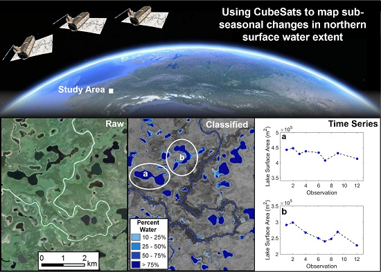
:Recent deployments of CubeSat imagers by companies such as Planet may advance hydrological remote sensing by providing an unprecedented combination of high temporal and high spatial resolution imagery at the global scale. With approximately 170 CubeSats orbiting at full operational capacity, the Planet CubeSat constellation currently offers an average revisit time of <1 day for the Arctic and near-daily revisit time globally at 3 m spatial resolution. Such data have numerous potential applications for water resource monitoring, hydrologic modeling and hydrologic research. Here we evaluate Planet CubeSat imaging capabilities and potential scientific utility for surface water studies in the Yukon Flats, a large sub-Arctic wetland in north central Alaska. We find that surface water areas delineated from Planet imagery have a normalized root mean square error (NRMSE) of <11% and geolocation accuracy of <10 m as compared with manual delineations from high resolution (0.3–0.5 m) WorldView-2/3 panchromatic satellite imagery. For a 625 km2 subarea of the Yukon Flats, our time series analysis reveals that roughly one quarter of 268 lakes analyzed responded to changes in Yukon River discharge over the period 23 June–1 October 2016, one half steadily contracted, and one quarter remained unchanged. The spatial pattern of observed lake changes is heterogeneous. While connections to Yukon River control the hydrologically connected lakes, the behavior of other lakes is complex, likely driven by a combination of intricate flow paths, underlying geology and permafrost. Limitations of Planet CubeSat imagery include a lack of an automated cloud mask, geolocation inaccuracies, and inconsistent radiometric calibration across multiple platforms. Although these challenges must be addressed before Planet CubeSat imagery can achieve its full potential for large-scale hydrologic research, we conclude that CubeSat imagery offers a powerful new tool for the study and monitoring of dynamic surface water bodies.

1. Introduction
Quantifying spatial and temporal variability in surface water area and storage is critical for effective water resource management, testing flood models, and assessing impacts of environmental and climatic change. In situ monitoring stations for lake water levels and river discharge are sparse and furthermore provide only one-dimensional point observations that acceptably characterize inundation and storage in well-defined, constrained bathymetries but not in complex floodplains and/or wetland environments [1]. In situ monitoring of shoreline boundaries is exceedingly rare, as are water level gauges in small lakes. While river gauges are common in cities and developed countries, they are sparse in other areas, particularly in the Arctic [1,2,3]. Remotely sensed measurements of surface water are consequently an essential supplement to ground measurements for measuring, monitoring and modeling global water resources [1,4].
Although mapping surface water extent using optical imagery is well established [1,5], a tradeoff between high spatial versus high temporal resolution sensors has traditionally prevented study of dynamic, fine-scale changes in surface water extent over short temporal scales. Surface water mapping has a long legacy with Landsat sensors (TM, ETM, OLI) due to their relatively high spatial resolution (30 m), high radiometric quality, and long term continuous record [6], yet their historical 16-day revisit time, typically lower due to cloud cover, limits the applicability of Landsat for tracking sub-seasonal patterns in surface water extent. The twin Sentinel-2 satellites now offer more frequent returns (5–10 days) at 10 m resolution, but cloud obscuration still lowers the actual revisit frequency. MODIS imagery is often used to study large, dynamic hydrologic systems such as rivers (e.g., [7]), wetlands (e.g., [8]) and lakes (e.g., [9]) due to its daily periodicity, but the coarse resolution of MODIS visible/NIR bands (250–500 m) means only coarse scale variability can be distinguished. Combining MODIS and Landsat observations can enable near-daily, 30 m land surface monitoring, though the results are sensitive to the blending algorithm used [10,11,12]. This compromise between high spatial and temporal resolution has thus limited the ability to track both fine-scale, sub-seasonal patterns in surface water extent.
High frequency observations of surface water extent are particularly critical for study of dynamic high latitude hydrologic processes. The high latitudes contain the highest proportion of small water bodies on Earth [13,14], nearly all of which are unvisited and unstudied. Due to strong seasonality, northern lakes and rivers are highly dynamic. Spring river ice breakup and associated peak flow and flooding can lead to rapid changes in surface water extent [15,16]. Such peak flow events are critical for recharging lakes and wetlands, transporting water through low-relief floodplains [8,17,18]. Warming Arctic temperatures have increased interest in understanding how surface water extent responds to thawing permafrost [19,20]. Permafrost acts as a barrier between the surface hydrologic system and the groundwater system, meaning that in discontinuous permafrost, the surface water and groundwater systems are connected where permafrost is absent but disconnected where permafrost is present [19,21]. In high latitude wetlands underlain by discontinuous permafrost, such as the Yukon Flats in central Alaska, decadal-scale analyses (>30 years) of interannual patterns in lake area have noted variable changes in surface water extent due to a combination of thawing permafrost, shortening spring duration of snow cover, changing water balance and underlying hydrogeology [22,23,24,25,26]. Despite evidence that sub-seasonal cycles strongly influence patterns in surface water extent, potentially obscuring climate-related trends [23], little research has focused on fine-scale, sub-seasonal variability in these areas, due to the absence of sufficient high resolution, high frequency imagery.
Recent development of small, affordable satellites known as CubeSats opens new possibilities for studying fine-scale, temporally dynamic hydrological processes from space. CubeSats are typically about the size of a bread box (0.003 m3), and contain little more than a four-band multispectral camera and power/downlinking equipment. Owing to their small size and low cost, CubeSat imagers can overcome the tradeoff between high spatial and high temporal resolution by deploying them in a multi-satellite constellation. This approach relies on both satellite mass production and declining launch costs, making CubeSats comparatively affordable for commercial satellite companies to launch and operate [27]. A notable example is Planet (formally known as Planet Labs; http://planet.com), a company that has successfully built and launched 281 CubeSats since 2013. With 148 CubeSats in sun-synchronous orbit, Planet currently images nearly all of the global land surface at 3–5 m resolution daily, providing near-real time imagery to paid and academic subscribers. This large volume of frequent, high resolution imagery holds potential value for hydrological applications because open water surfaces are among the simplest land covers to discriminate in visible/NIR imagery, and frequent observations are necessary to track dynamic hydrologic processes such as flood waves and river ice breakup. However, CubeSat imagery is acquired using inexpensive sensors which cannot achieve the same radiometric quality, consistency and signal-to-noise ratios of space agency-funded missions [28]. Together with the newness of CubeSats, prevailing concerns about cross-sensor calibration, image quality, geolocation accuracy, and data availability have limited the advent of CubeSat-based hydrological research. Despite the strong potential of frequent, high-resolution CubeSat imagery to transform hydrological remote sensing, such data remain generally untested and unproven within the hydrologic community [27].
Here, we present a first demonstration of the use of CubeSat imagery to track sub-seasonal changes in surface water extent. Using two types of Planet satellite imagery we tracked surface water inundation variations across a 625 km2 study region in the Yukon Flats, north central Alaska during summer 2016 as follows: First, we developed a non-binary water classification method for Planet imagery (adapted from [29]) and validated it with concurrent WorldView-2 satellite images; second, we analyzed sub-seasonal patterns in lake and river surface areas and their sensitivity to measured discharge variations in the Yukon River; finally, we assess Planet’s anticipated future imaging capabilities and discuss some potential applications and limitations that must be addressed before CubeSat imagery can be widely used in hydrologic research.
2. Study Area and Data
2.1. Study Area
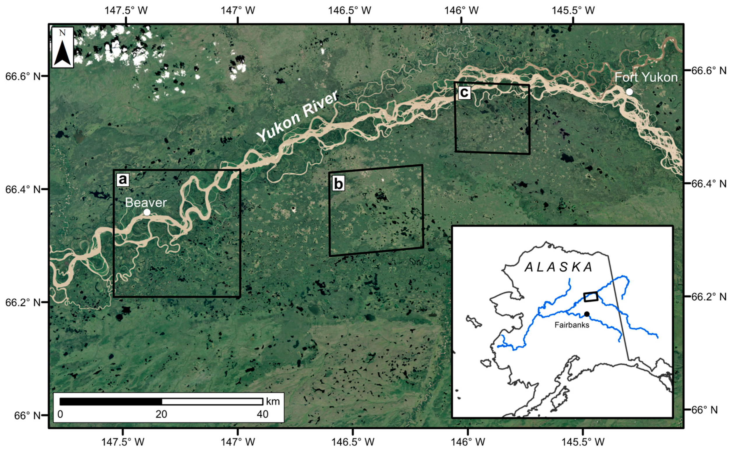
A 625 km2 study area (centered at 66.3 N, −147.4 W) was selected within the Yukon Flats, a dynamic wetland system in north central Alaska surrounding an extended low-relief section of the Yukon River (Figure 1). This defined area contains >450 lakes and a 30 km section of the Yukon River, as well as the small settlement of Beaver, AK (Figure 1, box a). We also performed lake area validation in two other subareas in the Yukon Flats (Figure 1, box b,c). The Yukon Flats are characterized by extremely cold winters (mean January air temperature of −23 °C) and warm, dry summers (mean July air temperature of 17 °C) with low annual precipitation (26.7 cm water equivalent on average) [23]. The study area is primarily covered by spruce and birch forest and marshland and is underlain by discontinuous permafrost [23,30,31,32]. Lakes in the Yukon Flats typically depend on recharge from spring river ice breakup flooding events [23]. In recent years several studies have analyzed long-term inter-annual trends in surface water extent to assess a potential role of thawing permafrost [22,23,24,25,26].
2.2. Remote Sensing Data
Planet currently distributes three types of imagery, RapidEye, PlanetScope, and SkySat, two of which are studied here (Table 1). RapidEye refers to a constellation of 5 satellites (dimensions 0.8 m × 0.94 m × 1.2 m) launched in 2008 by German company RapidEye AG and now acquired and operated by Planet. RapidEye imagery has 5 bands, blue (Band 1, 440–510 nm), green (Band 2, 520–590 nm), red (Band 3, 630–685 nm), red edge (Band 4, 690–730 nm) and near infrared (Band 5, 760–850 nm) and a ground spatial resolution of 6.5 m. PlanetScope is a constellation of 120 smaller CubeSats known as ‘doves’ (dimensions 10 cm × 10 cm × 30 cm) built and operated by Planet, and launched in groups called ‘flocks’. PlanetScope imagery has four bands, blue (Band 1, 455–515 nm), green (Band 2, 500–590 nm), red (Band 3, 590–670 nm) and near infrared (Band 4, 780–860 nm) and a ground spatial resolution of 3.7 m. Skysat imagery has four bands (blue, green, red and NIR) and a ground resolution of 0.8 m. As it is a constellation of 13 satellites, however, SkySat currently captures imagery only over tasked areas (typically urban and developed areas). It was not available to this study and therefore excluded from the analysis.
For both RapidEye and PlanetScope we analyzed the Planet Level 3A data product (“Analytic Ortho Tile Product”) which is a mosaic of multiple images from the same swath aggregated into uniform 25 km × 25 km tiles. This product is projected to UTM coordinates and orthorectified using GCPs and fine-scale DEMs to a positional accuracy of <10 m RMSE [33]. Planet Level 3A imagery is also converted to absolute radiometric values using calibration coefficients that are monitored and updated for each satellite (see Section 5.2). Following radiometric calibration [33], the Level 3A product has 16-bit spectral resolution. RapidEye and PlanetScope data availability was irregular in summer 2016, when Planet’s multi-satellite flocks were in early stages of deployment. Therefore, the revisit rates presented in this study are irregular and less frequent than current revisit rates at full operational capacity. We examined all RapidEye and PlanetScope imagery in one Planet tile (No. 0669714) collected in summer 2016, which due to data availability limitations ranges from 23 June to 1 October (Table 2). To validate our water extraction method, we also used panchromatic WorldView-2 and WorldView-3 imagery operated by DigitalGlobe (Table 2). The panchromatic band (450–800 nm) has a ground resolution of 0.5 m (WorldView-2) and 0.3 m (WorldView-3).
2.3. River Discharge
In situ river discharge data for the Yukon River was obtained from the USGS station located in Eagle, Alaska, approximately 400 km upstream of our study area. We created a discontinuous time series of daily discharge measurements corresponding to each remotely sensed date of observation. While a simplification of the discharge time series, this approach facilitated a useful comparison between remotely sensed river width and in situ discharge.
3. Methods
3.1. Water Classification
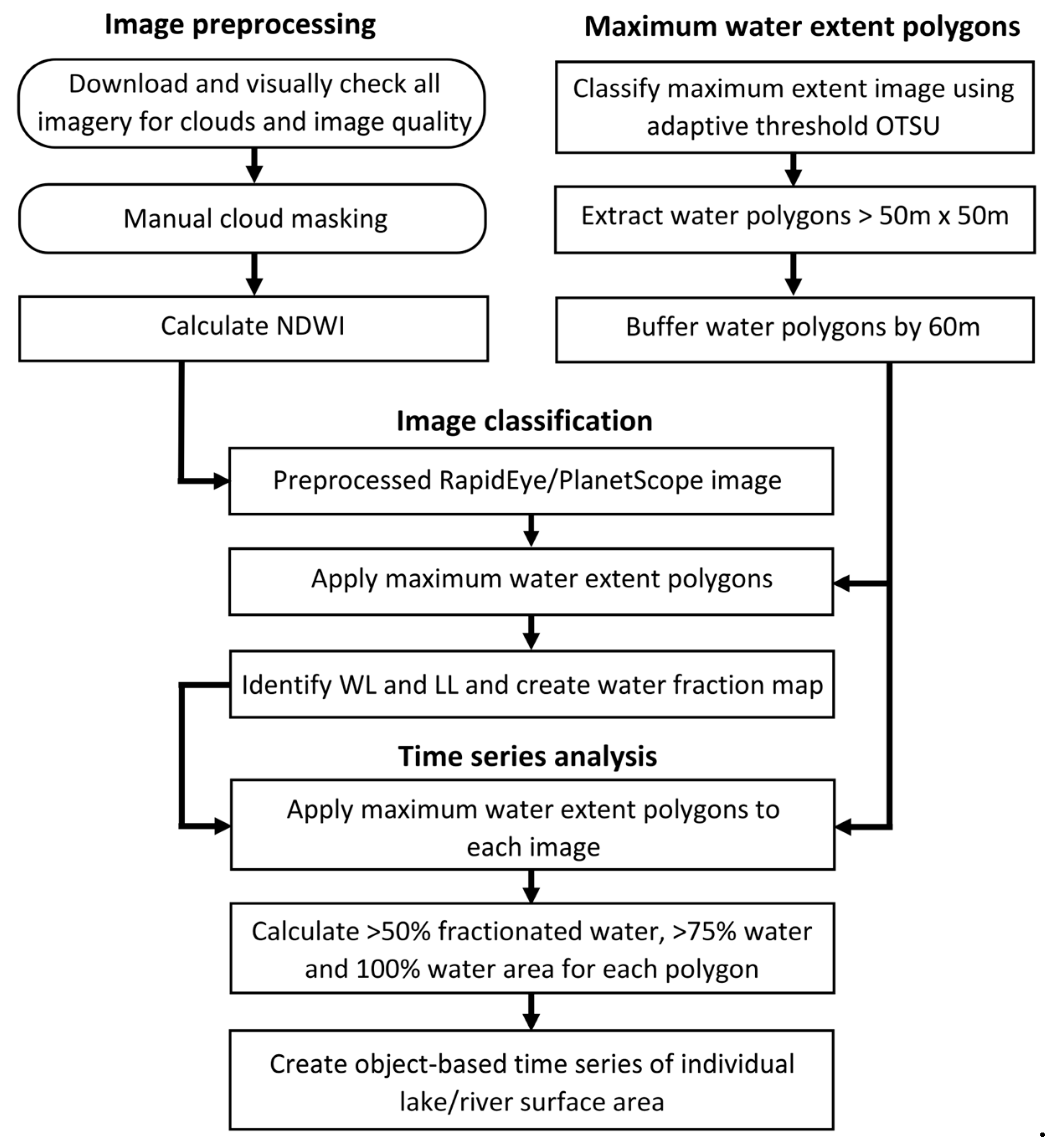
To classify open water from surrounding land and vegetation, a 10-step procedure was used (Figure 2). First, Planet imagery were manually checked for clouds. Although Planet does provide a cloud index value indicating the percent of cloud-covered pixels for each image, the index performance is not consistent in snow and ice conditions at present and a cloud mask product is still unavailable. For every image where clouds were present, cloud cover and cloud shadow masks were manually digitized and masked out. We ignored all imagery with a solar zenith angle greater than 78 degrees or with cloud cover greater than 70%. We then calculated a Normalized Difference Water Index (NDWI) for each image, defined as the difference between the green and near-infrared reflectance (Band 2–Band 5 for RapidEye, Band 2–Band 4 for PlanetScope) divided by the sum of the green and near-infrared (Band 2 + Band 4/5) [34]. This yields an NDWI index value between −1 and 1, where open-water pixels approach 1 and are more easily distinguishable from non-water pixels.
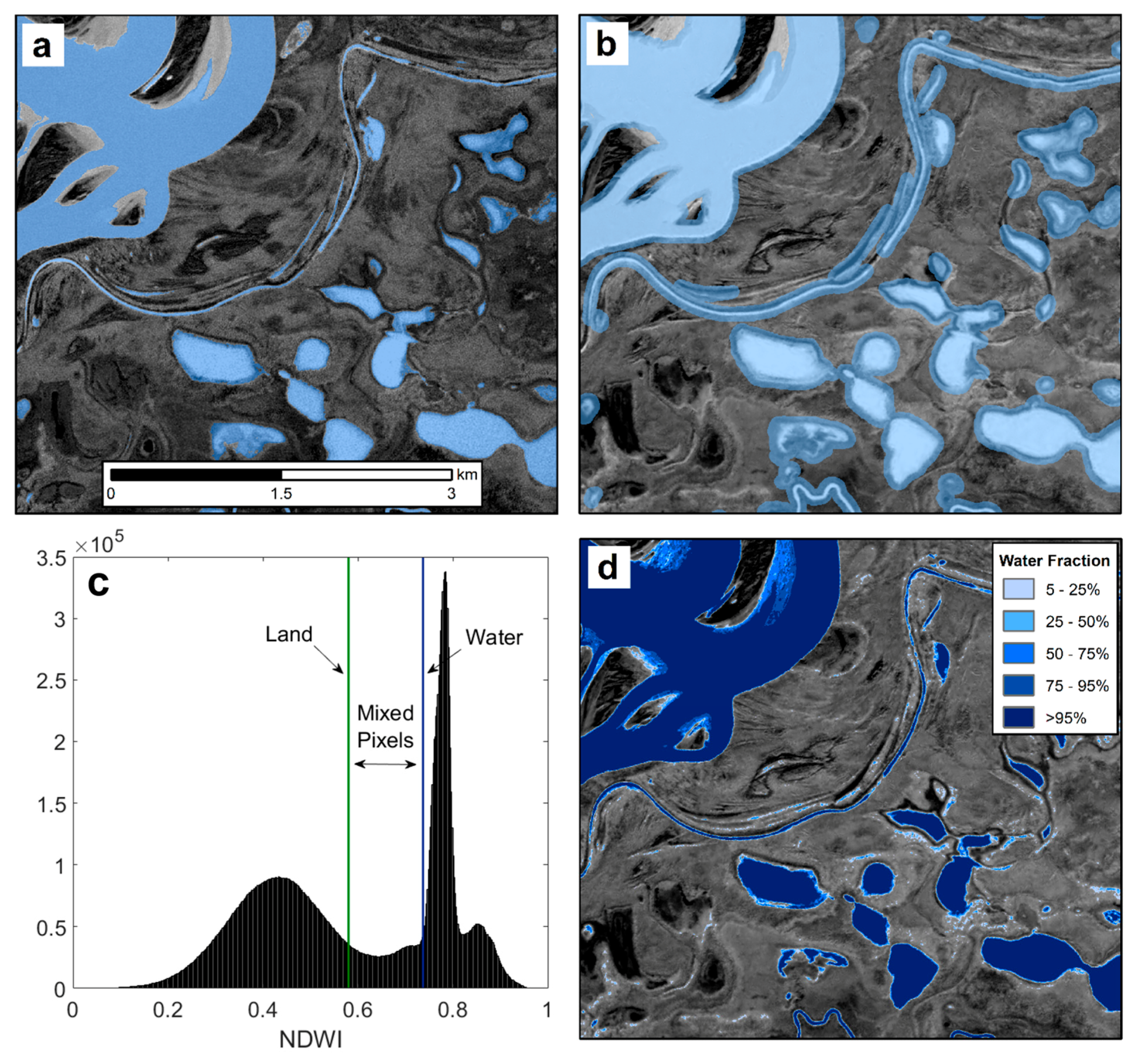
For water classification, we used a water fraction approach adapted from [29], who originally applied this method to shortwave infrared (1550–1750 nm) Landsat TM and ETM+ imagery. In complex floodplain environments such as the Yukon Flats where inundated vegetation and mixed land/water pixels are common, a multi-step, non-binary water classification enables more accurate water area extraction through accounting of fractionated water pixels [29]. First, Otsu adaptive thresholding [35] was used to delineate potential water bodies in a maximum extent image to create an initial water mask (Figure 3a). All water bodies less than 2500 m2 were removed from this initial mask. The water mask was then dilated using a 60 m disk object and converted to polygons, yielding an initial buffered polygon mask containing both the maximum extent of the water body and some surrounding land and vegetation [29]. These buffered lake polygons were then intersected with the NDWI for each image, generating a histogram of NDWI pixels within the buffered water mask (Figure 3b).
The water fraction of each pixel was then determined by applying dynamic land and water thresholds to each image [29]. The buffered water histograms typically have two peaks, one characteristic of land pixels (lower NDWI) and the other of water pixels (higher NDWI). We identified the 100% land threshold (LL) and 100% water threshold (WL) as:
where and are the heights of the land/water peak respectively and and are to the prominences of the land/water peaks. We then calculated the water fraction (WF) for each pixel as [29]:
The water fraction is thus the percent of each pixel that is inundated or water covered and is particularly useful in this region where many pixels contain inundated vegetation. All NDWI pixels ≥WL were considered 100% water and all NDWI pixels <LL were considered 100% land.
3.2. Time Series Analysis
Following generation of water fraction maps, we tracked lake and river surface area changes over the late summer season. Due to the presence of clouds and varying swaths and pixel sizes of Planet imagery, an object-based approach was used to track changes in lake and river extent, with each water body treated as an individual object. This approach is well-suited for time series analyses involving different sensors and ground resolutions and additionally limits the impact of potential geolocation error. To do this, we first reapplied the maximum extent buffered polygons to each water fraction map and calculated the total area of pixels within each polygon that are 100% water and greater than 75% water for each image. We also determined the total >50% fractionated water area within each polygon by summing the pixel values for all pixels greater than 50% water. This created a sub-seasonal time series consisting of three different lake areas for each lake observation (>50%, >75%, 100%). We primarily used >75% area for our time series analyses but observed temporal patterns are similar for all three metrics. We analyzed changes in river surface area by examining seven individual river reaches ranging from 2.5 to 3.5 km in length. To better facilitate comparison between reaches, river surface area was converted to effective width (We) [5,36,37] by dividing by the length of each river reach. If multiple PlanetScope image acquisitions were acquired on the same day, we assigned the largest observed lake area or river We to that day. Finally, to illustrate large-scale changes in inundation extent, we produced pixel-based water fraction change maps between three cloud-free RapidEye images representing early (23 June), mid (17 August) and late (1 October) season.
3.3. Validation of Planet Water Fraction Maps
A key component of assessing the utility of Planet imagery for water mapping is determining whether surface water area can be reliably and automatically extracted from CubeSat imagery. We validated our Planet imagery water fraction maps by comparing them to lake shorelines delineated manually from one WorldView-2 and two WorldView-3 panchromatic images acquired on 30 August and 8 September 2016 (Table 1). WorldView-2 and WorldView-3 offer high radiometric stability and finer spatial resolution (0.5 m, 0.3 m respectively) than RapidEye and PlanetScope imagery, and have been previously demonstrated to yield high-quality mapping of surface water [38,39]. We delineated 48 lakes from the September 8 image and 45 lakes from the 30 August image, and compared them to our water fraction classification of one 8 September RapidEye image (Figure 1 inset c) and three 2 September PlanetScope images (Figure 1 inset b), respectively. We compared 100% water area, >75% water area and >50% fractionated water area with the manually delineated WorldView area (Figure 4 and Figure 5).
Geolocation error is also thought to affect CubeSat imagery due to the small size of the satellites and possible orbital drift. To assess image geolocation accuracy, we reprojected the manually delineated WorldView lakes to WGS84 UTM Zone 6N to correspond with Planet’s gridding system. We then calculated the centroids of both the manually delineated WorldView lakes and RapidEye/PlanetScope-derived lakes and compared the centroids of the WorldView lakes to the centroids of the RapidEye/PlanetScope lake boundaries outlining >75% water area.
4. Results
4.1. Detection of Surface Water
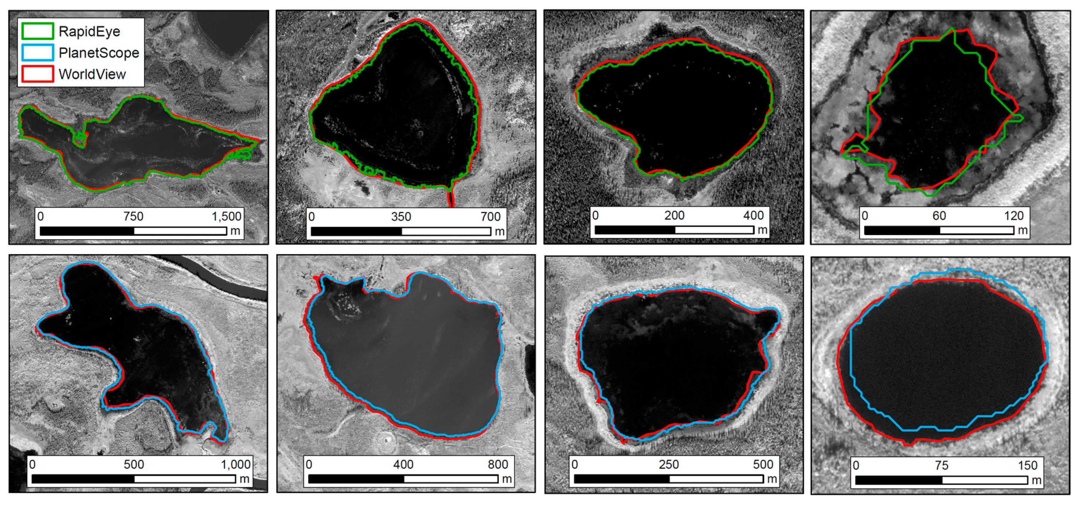
We find strong agreement (r2 > 0.99) between lake boundaries manually delineated in high-resolution WorldView-2 and WorldView-3 images and water fraction classifications derived from Planet RapidEye and PlanetScope imagery (Figure 4). The normalized root mean square errors (NRMSE) vary from 5.7% to 18.7% for RapidEye, with >75% area showing the best agreement (NRMSE = 5.7%) with WorldView images (Figure 4). The NRMSEs vary less for PlanetScope, ranging from 10.9% to 12.6%. While the WorldView and RapidEye images are contemporaneous (taken 2 min apart), the three days between WorldView and PlanetScope image acquisitions may be responsible for the higher RMSEs for PlanetScope. The mean Euclidean distance between Planet and WorldView lake centroids is 9.8 ± 4.1 m for RapidEye and 10.5 ± 3.2 m for PlanetScope, comparable with the <10 m ground location accuracy Planet claims for its imagery [33]. This analysis was only performed for lakes where the classifications yielded similar lake geometry and thus the difference between the centroids primarily represents a geolocation offset rather than classification error. However, for all lakes, some of the offset may derive from classification differences, meaning our reported geolocation errors are conservative estimates of the actual offset. The direction of the offsets varies between different images but is generally consistent within a single image (Figure 5). For the 2 September PlanetScope image, the offset primarily trends northeast, with azimuths for individual lakes ranging from due north to due east. For RapidEye the offsets are more variable between lakes but generally trend within 45° of due north. In sum, combined, the ~10% NRMSEs and 10 m ground offsets suggest water area can be reliably extracted from Planet imagery within reasonable error.
4.2. Temporal Changes in Water Inundation Area
Over the course of the mid to late summer season (23 June to 1 October) we identified a total of 470 lakes >2500 m2 within our 625 km2 study area. These water bodies received between 4 and 9 cloud-free Planet observations over this period, with an average of 6.0 cloud-free observations. The maximum observed lake area is 1.23 km2, and for all lakes >2500 m2, the mean maximum lake size is 0.0735 km2 or 73,470 m2. On average, the studied lakes lost 0.028 km2 of surface water area, or 63% of their maximum observed area over the summer season. However, not all water bodies followed this average trend, with some shrinking, some expanding, and others stable. Because a lake’s areal change tends to scale with its area [40], we divided lakes into two categories, i.e., 2500 m2–10,000 m2 and lakes >10,000 m2. On average, lakes <10,000 m2 lost 4280 m2 or 79% of their maximum observed area as the summer progressed, whereas lakes >10,000 m2 lost 42,900 m2 or 52% of their maximum area. The normalized variability for each lake, which we defined as the mean change in lake area between each observation, decreased significantly with area. For all lakes >2500 m2, the mean variability is 47%, but the mean variability is 67% for lakes between 2500 m2 and 10,000 m2, and 33% for lakes >10,000 m2.
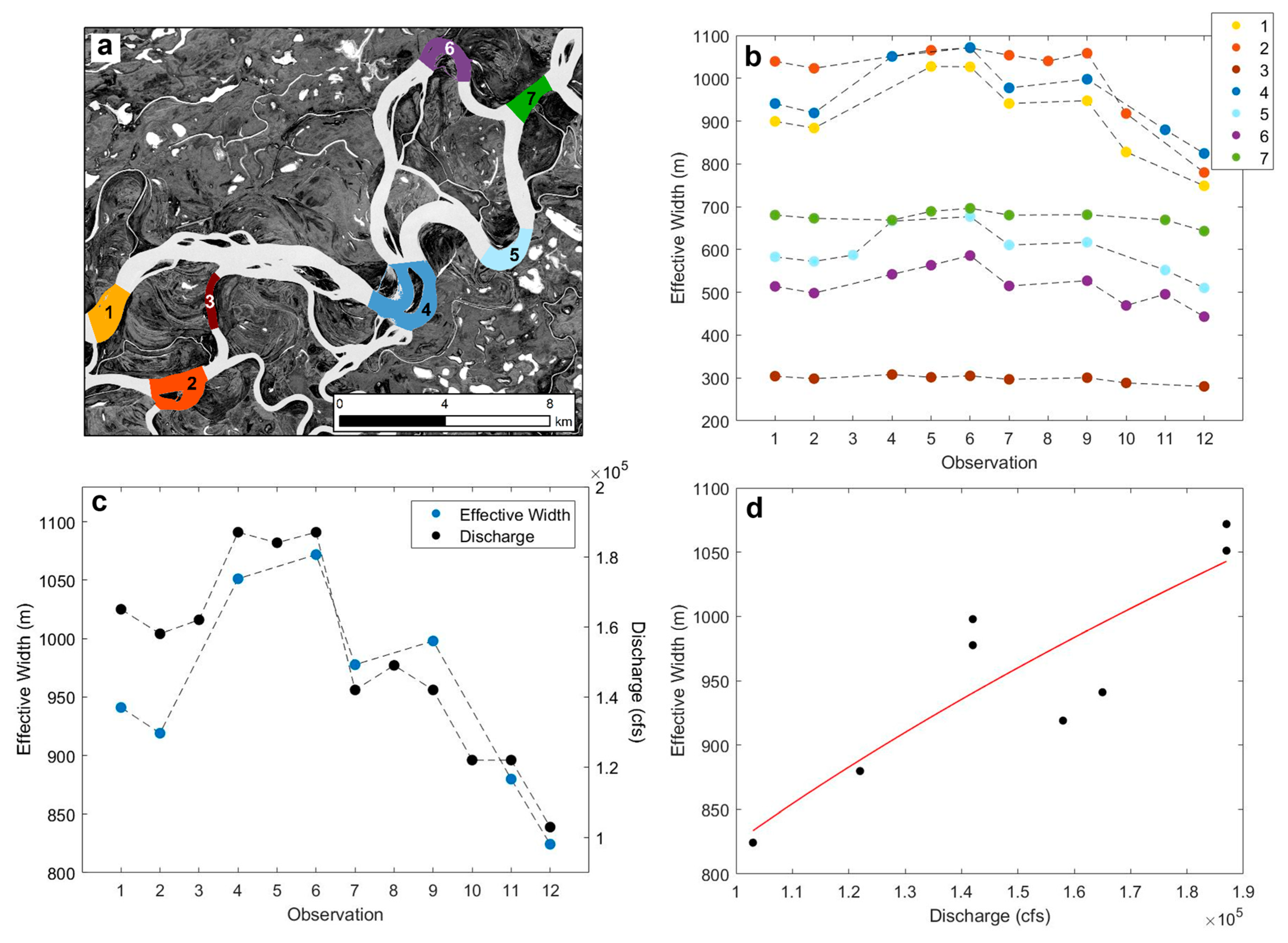
Yukon River effective width We varied most strongly on wide reaches surrounded by sediment bars and least on narrow constrictions (Figure 6a,b). Effective widths of Reach 3 and Reach 7 changed little over the observation period, whereas other reaches increased in mid-August (observations 4–6, Figure 6b,c) before decreasing to a seasonal low in October. Effective width is correlated with discharge [5,7,36,37,41] so to assess the validity of Planet We measurements we compared them with Yukon River discharge data from the USGS station at Eagle. We find that a daily discharge time series corresponding to our dates of observation correlates well with our effective width measurements, yielding an r2 of 0.75 (p < 0.01) (Figure 6c,d).
While most of the Yukon Flats lakes studied here decreased in surface area over the observation period, heterogeneous patterns of lake area increase and stability are also evident (Figure 7). Overall, 83% of the studied lakes decreased in area between 23 June and 1 October 2016, with 22% losing at least half of their surface area. Between 23 June and 17 August, however, 56% of lakes increased in surface area, and 89% of lakes shrunk between 17 August and 1 October. This summertime peak in mid-August and subsequent decrease in surface extent exhibited by more than half of lakes is also reflected in the time series of river effective width (Figure 6), signifying hydrologic connectivity of these lakes to the main-stem Yukon River.
In low-relief wetland environments where a small change in water level can cause a large change in inundation extent, temporal correlations between changing river discharge and individual lake surface areas are indicative of floodplain connectivity [8]. To quantify these correlations, for each lake object with at least 5 satellite observations and an observed maximum area >10,000 m2, we calculated Pearson’s R between the Yukon River discharge at Eagle and Planet time series of surface water extent [8]. Of the 268 lakes meeting these requirements, 100 (37%) are correlated with Yukon River discharge at the 90% confidence level and 60 (22%) are correlated at the 95% confidence level.
Using a non-parametric Mann-Kendall test [42] we also assessed how many of these 268 lakes display statistically significant trends over the summer season. We find 65 (24%) of lakes have a statistically significant (p < 0.1) decreasing linear trend over the summer season, 2 (1%) display increasing trends, and 201 (75%) display no trend. As nearly all lakes decreased in extent, the percent of lakes with statistically significant trends reflects lakes which changed linearly with little bidirectional variability between observations.
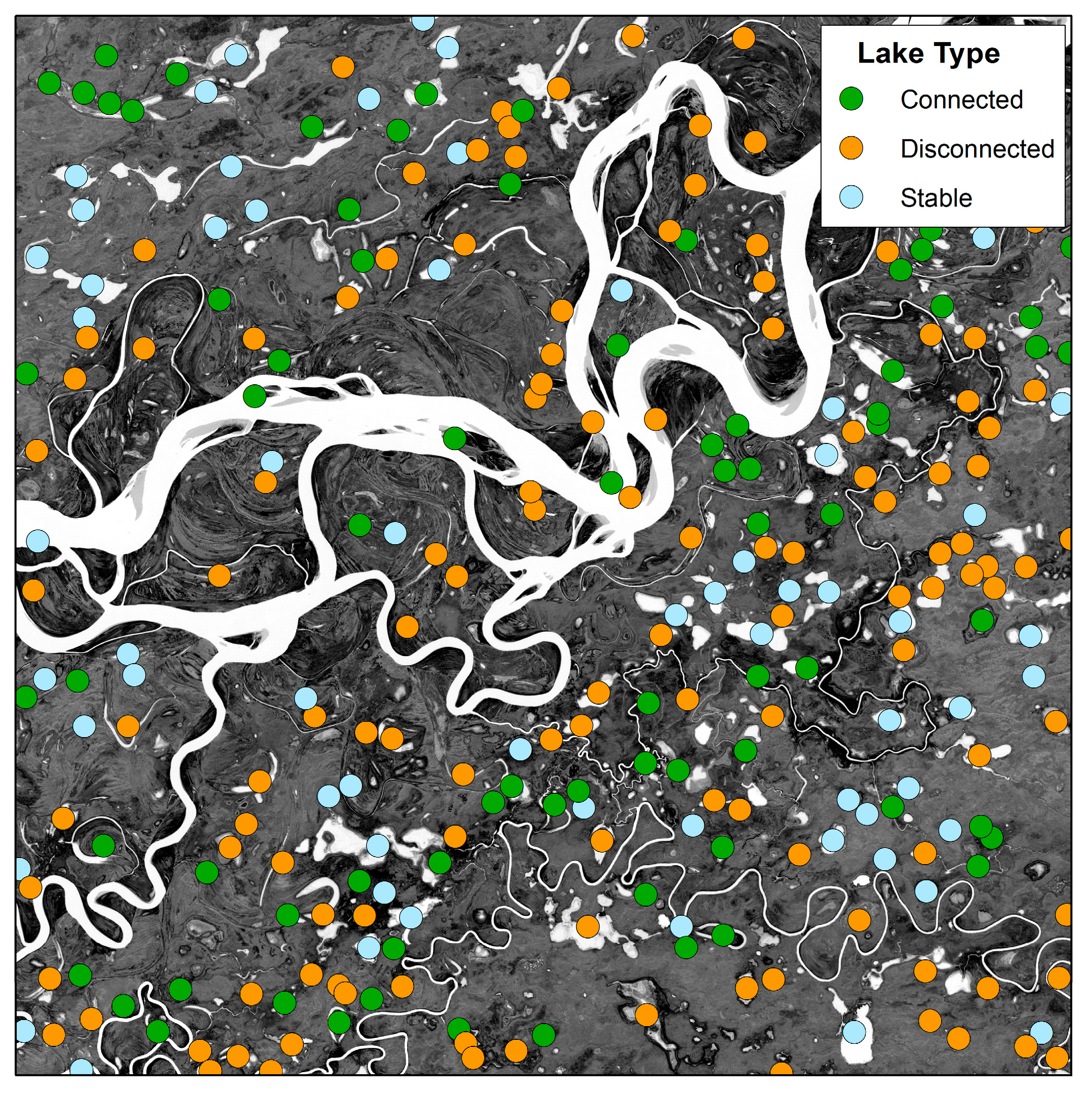
Based on the observed correlation to river discharge, we characterized the 268 study lakes into three categories: connected, disconnected and stable, examples of which are shown in Figure 8. Connected lakes are interpreted as being hydrologically connected to the Yukon River [8] and thus immediately responsive to changes in its discharge. Here we defined connected lakes as having a surface area standard deviation >10% and a statistically significantly (p < 0.1) correlation to river discharge. 77 lakes (28%) were classified as connected. In some cases, such as the example shown in Figure 8b, there may be a visible channel connecting the lake to the river system, but in many connected lakes no such channel is visible in the imagery. Disconnected lakes are uncorrelated with river discharge, but still experience substantial area changes over the summer season. These lakes typically steadily decrease in surface area throughout the summer season and do not respond to the summer high stage event. Here they were defined as lakes with a surface area standard deviation >10% and no correlation to Yukon River discharge, with 128 lakes (48%) classified as disconnected. Finally, stable lakes are interpreted as being hydrologically disconnected from the Yukon River water, possibly due to steep embankments, sills or other topographic controls, and/or sustained by connections to groundwater. They were defined in this study as lake objects having a surface area time series standard deviation of less than 10%, totaling 63 lakes (24%). There is no clear spatial pattern explaining the distribution of the different lake types, though we do observe some spatial clustering of lakes of the same type (Figure 9).
5. Discussion
5.1. Assessment of Planet Imagery
5.1.1. Utility of Planet CubeSat Imagery for Tracking Surface Water Dynamics
This study demonstrates that Planet imagery is suitable for mapping and tracking changing inundation extent of hundreds of small, heterogeneous water bodies in a complex, dynamic wetland region. We find the surface areas of small water bodies can be reliably and automatically extracted from both RapidEye and PlanetScope imagery, with a mean NRMSE of ~11%. While the nominal ~10 m geolocation error of Planet imagery [33] will likely cause difficulties for comparing Planet imagery to other fine-scale map products and/or field measurements, our treatment of water bodies as fuzzy-geolocation objects mitigates this error for time-series analysis purposes, and a geolocation offset of <10 m is sufficient for analysis of lakes >2500 m2. Furthermore, this geolocation error is a systematic offset (though with inconsistent directions between images) and would thus be correctable through a simple transformation. The strong correlation between Yukon River effective width and discharge (Figure 6), further highlights Planet’s utility for obtaining useful sub-seasonal hydrologic measurements from space.
5.1.2. Limitations and Challenges
Several important limitations remain to be addressed before CubeSat imagery can be fully implemented into larger-scale hydrological observing systems. Currently, a serious limitation is lack of a cloud mask or a regionally/globally applicable automated cloud masking algorithm derived from Planet imagery. Automated cloud detection in multi-temporal visible/near-infrared satellite imagery is non-trivial [43] and will be particularly challenging with PlanetScope given only four bands and variable quality imagery. Until an automated cloud masking product or algorithm is developed, researchers must manually remove clouds which generally precludes broad-scale, high-resolution applications including surface water mapping. While minor, the observed geolocation error, combined with the narrow swath width of Planet CubeSat imagery, make differencing difficult at fine spatial scales (i.e., 50 m × 50 m lakes). Use of an object-based approach (Figure 3 and Figure 7) mitigates but does not fully eliminate this problem.
Additional limitations associated with CubeSat imagery derive from its inexpensive sensors and multi-satellite constellation approach. PlanetScope imagery is calibrated to a radiometric uncertainty across satellites of 5–6% at 1-sigma [44] and RapidEye is calibrated to 4% uncertainty [45]. These values compare reasonably to Landsat at-sensor calibration uncertainty, which ranges from 3% (OLI) to 5% (TM and ETM+) to 10% (MSS) [46,47,48]. However, to enable daily or near-daily high resolution observations of the entire globe, Planet is presently operating 148 satellites in sun-synchronous orbit, meaning a collection of images of the same location likely come from many sensors. While all imagery is calibrated, Planet image quality, including signal to noise ratio and exposure, can vary between sensors, a non-trivial error source when time series analyses involve imagery from tens of sensors [44]. Figure 10 illustrates this variability in near infrared and NDWI for water bodies and surrounding wetlands in five PlanetScope images taken within a 10-day period in 2016. Though some of the observed differences may be due to atmospheric scattering and absorption, the non-linearity of between-image offsets suggests radiometric calibration and/or sensor variability is likely the cause.
The lack of atmospherically corrected Planet imagery also complicates the interpretation of time series analyses, particularly those involving global radiance thresholds or complex land surface classifications [28]. Fully automated time series analyses using Planet data may thus require dark body atmospheric correction [49], adaptive thresholding as demonstrated here, or combination with other sensors [28]. The narrow range of the electromagnetic spectrum sampled by Planet’s sensors (455–860 nm) also limits utility of the resulting imagery. For example, variability in shortwave infrared (1400–3000 nm) is critically important for distinguishing between cloud, snow, ice and water surfaces [50], thus restricting the types of observations that can be made from Planet imagery in areas where snow occurs. Given these issues, hydrological applications of Planet imagery should presently be limited to relatively simple classifications, such as water mapping, which do not require atmospheric correction or rely on predefined radiance thresholds. All imagery classified in this analysis was visually checked and in general our automated classification method performed well for all imagery, suggesting image quality problems can be minor. However, further research is needed to examine radiance variability between different PlanetScope satellites and the effect this has on different types of classification. For example, combining PlanetScope imagery with Landsat-8 surface reflectance products may reduce cross-sensor calibration error [28]. Furthermore, a PlanetScope surface reflectance product produced from tandem observations with other sensors is now being tested and available in Beta as of 1 October 2017 and may allow more rigorous analyses [33].
Despite the above issues, specific methodological considerations can overcome some of them to enable robust hydrological analyses. First, water classifications based on a band ratio index such as NDWI is better suited for Planet analyses as it precludes the need for atmospheric correction [51]. We also advise against the use of global/stable thresholds due to cross-sensor variability. Perhaps the most critical methodological step is object-based time series analysis. By assigning the water extent change as an attribute to the lake polygon, and ignoring small temporal changes in lake location, problems of small image offsets and mismatched water edge boundaries are avoided. This approach is particularly important for Planet analyses due to geolocation uncertainty, the use of multiple sensors and varying resolution and swath coverage of the imagery. We therefore still conclude that Planet imagery is valuable for tracking rapid, fine scale changes in surface water extent, particularly as observation frequencies reach the company’s near-daily imaging capacity [33].
5.2. River-Floodplain Connectivity of the Yukon Flats
The high spatial and temporal resolution of Planet imagery, accompanied by the non-binary classification method’s ability to detect water extent in the variable quality data make Planet imagery particularly useful for study of complex, dynamic surface water systems. Floodplains and wetland environments are dependent on hydrologic recharge from rivers, precipitation and groundwater flow. However, the relationship between floodplain inundation and changes in main stem discharge is not well understood due to the complexity of flow patterns and limited in situ observations of large wetland regions [8,52]. In high latitude wetlands such as the Yukon Flats, permafrost can further complicate these patterns by acting as a barrier between the surface and groundwater systems [13,19,20,24,53,54]. While the summer 2016 Planet acquisitions lack sufficient temporal sampling to fully address these questions, the observed patterns nonetheless enable general characterization of floodplain connectivity across our Yukon Flats study area (Figure 8 and Figure 9).
The divergent and spatially variable changes in lake surface area observed between 23 June and 17 August (Figure 7) suggest that surface water extent in the Yukon Flats is driven by a combination of the seasonal runoff cycle (i.e., spring snowmelt flooding and recharge, followed by summer drying), connections with the Yukon River main-stem, localized topography/bathymetry [40] and substrate conditions (i.e., permafrost, geology). Previous analyses of hydrologic connectivity in other floodplain systems may help explain these patterns. While conceptual models commonly assume floodplains to have a uniform “bathtub” response to changing main-stem river stage, floodplain inundation is complex, driven by distributary channels, floodplain topography and storage in wetlands and lakes [52,55]. In their analysis of the relationship between lake levels and inundation extent in the Peace Athabaska Delta, Pavelsky and Smith (2008) find that water levels in the floodplain do not reflect water levels in the river. They observe a dichotomy between the distributary channel network and the surrounding lakes and wetlands wherein channels within the network respond to changes in river level but summertime peak flow events have little impact on the lakes and wetlands. In contrast, Alsdorf et al. (2005) present a diffusion model to explain how distance from the river channel controls the response of floodplain water levels to changes in main-stem river stage. Our findings do not support either a dichotomy between channel network and wetlands or a diffusion model; instead we observe larger scale variability wherein roughly one quarter of lakes respond to changes in river level, one half drain over the course of the season and one quarter are stable. The spatial patterns of this variability do not reveal any clear drivers of lake behavior (Figure 10). While a few lakes which respond strongly to August high stage events are clearly connected to the river system, in general there is no mechanism distinguishable in the imagery able to explain these differences. In their analysis of a flood-wave event in the Amazon basin, Alsdorf et al. (2007) observe a complex pattern of temporal changes in water level wherein variations in water height can be highly localized and the flow path cannot be predicted directly from bathymetry alone. Our observed patterns perhaps fit better with this result, where the spatiotemporal complexity of floodplain connectivity impedes characterizing or predicting individual lake response through a model or conceptual framework. An added contributor for the observed heterogeneity in lake area changes may be substrate geology, as recent work has shown lakes located farther from the floodplain, along permeable alluvial terraces or over coarser soils, are more likely to experience long-term shrinkage [23,56,57].
A regional mechanism for the observed pattern of stable and decreasing lakes co-existing in close proximity may be the influence of permafrost, which occurs discontinuously within our study area [32]. The presence of permafrost tends to impede infiltration of lake water to groundwater systems, plausibly contributing to lake stability in this area. Development of taliks (thaw bulbs) beneath lakes promotes infiltration, and permafrost research has identified through-talik formation and permafrost degradation around some lakes in the Yukon Flats [24,31,58]. Lakes underlain by through-taliks are connected to the groundwater system, enabling water loss to the sub-surface [19,21,54]. The spatially heterogeneous patterns in surface water extent may thus be associated with discontinuous permafrost, though we observe no evidence of large lakes draining completely during the summer season.
In sum, we conclude that hydrologically connected lakes respond primarily to changing water levels in the main-stem Yukon River, whereas the sub-seasonal dynamics of other water bodies in the surrounding Yukon Flats wetlands are more complex, owing to a combination of intricate flow paths, underlying geology, and permafrost. According to the long-term (1951–2016) Yukon River discharge record at Eagle, the flow in 2016 was higher than average but well within normal variability, suggesting our observed results reflect sub-seasonal inundation patterns in wet years. Given the improving temporal frequency of Planet imagery, we anticipate future research can combine even denser time series of lake surface area with river discharge observations and maps of substrate geology and permafrost to improve scientific understanding of the controls on inundation in Arctic and sub-Arctic wetlands. Our observed variability further highlights that sub-seasonal patterns may obscure long-term trends in lake extent, the magnitude of which is often much smaller than sub-seasonal cycles driven by spring recharge, precipitation and late summer high discharge events [26,59]. Considering the interest in understanding long-term temporal changes in surface water extent in the Yukon Flats (e.g., [20,22,23]) and other high latitude environments (e.g., [17,31,56]), this variability can critically impact reported trends in lake extent, especially when observed patterns are based on only a handful of images per year. We therefore also suggest that spatially heterogeneous intra-seasonal variability needs to be considered in long-term trend analyses.
5.3. Future Applications of Planet Imagery
5.3.1. Anticipated Growth in Planet CubeSat Image Acquisitions
Despite the limitations discussed here, the high temporal and spatial resolution of Planet imagery makes it a unique and valuable remote sensing resource. At the time of writing Planet currently operates 148 satellites in sun synchronous orbit, yielding <1 day revisit capacity globally. Owing to orbit convergence, imaging capacity is highest at high latitudes. Here, we simulated both revisit rate and the probability of cloud-free collection when all launched satellites have been phased into staggered sun synchronous orbit. When all satellites are operating at full capacity, the expected revisit time will be sub-daily at high latitudes, and the cloud-free collection probability for most high latitude locations is likely to be between one and three days (Figure 11). Planet plans to maintain a stable imaging capacity in sun synchronous orbits by regularly replenishing the constellation with new deployments.
5.3.2. Other Hydrological Applications
With daily or near-daily acquisitions, Planet CubeSat images therefore hold potential to substantially impact hydrologic research, for example in data assimilation, flood monitoring and prediction, and floodplain connectivity. Data assimilation is critical for driving hydrologic models and typically involves interpolating ground-based or remotely sensed observations to improve model performance, providing complete estimates of a poorly-measured geophysical parameter or organizing/removing valuable/redundant information [60]. For example, retrievals of surface water fraction and snow cover obtained from Planet CubeSat imagery could be assimilated into regional hydrologic models. Merging time-series of CubeSat inundation maps with water surface heights from satellite altimeters would create large-scale observations of surface water storage [61]. Finally, the fine spatial resolution and anticipated near-daily availability of Planet CubeSat data should facilitate downscaling of coarser resolution satellite observations for regional and local hydrologic models [62]. High frequency Planet CubeSat imagery should also prove valuable for refining and calibrating flood prediction models [63], and with near-time capability assist in disaster relief efforts [64,65].
Another clear application for Planet CubeSat imagery is remote estimation of river discharge from space. Deriving satellite retrievals of river discharge is an active research area within the hydrologic community, owing to the sparse network of in situ discharge gauges outside of the continental United States and Europe and the critical need for discharge measurements for global resource monitoring [4]. A number of different methods have been developed to estimate discharge from optical satellite imagery, often building statistical relationships between river width/extent both with and without in situ measurements [5,66,67,68,69,70]. A major limitation of current remotely-sensed discharge estimates is the lack of sufficient temporal sampling of high resolution imagery due to revisit time or cloud cover [68]. While Planet imagery is still subject to cloud obscuration, its projected high imaging capabilities will enable more frequent cloud-free observations than traditional sensors and allow discharge estimation for more rivers than coarse-resolution MODIS.
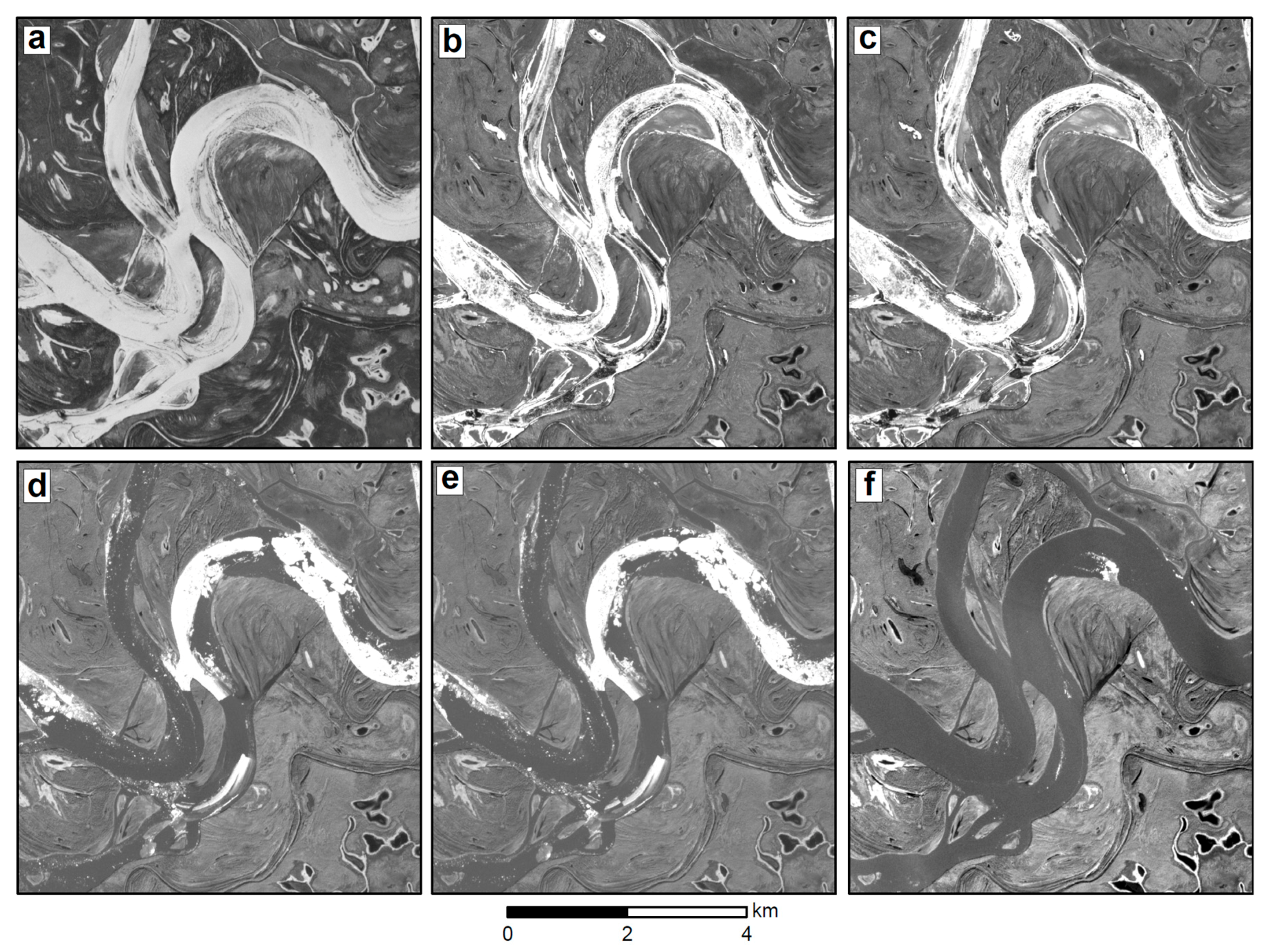
Planet CubeSat imagery is particularly valuable at high latitudes where orbits converge, surface water is both dynamic and abundant, and in situ observations are sparse. Northern rivers are critical not only for Arctic ecosystems but also for the global climate system, as increasing runoff to the Arctic ocean can impact ocean circulation patterns [71,72]. However, rivers tend to be braided or anastomosing at these latitudes, making in situ monitoring especially difficult. Estimating discharge of large high latitude rivers such as the Yukon is therefore an obvious, critical application of Planet imagery. Planet imagery is also well-suited for mapping and tracking river ice breakup. Analyses of river ice breakup timing have typically relied on ground-based measurements [73,74] which do not enable understanding of how ice breakup progresses downstream through space and time. While satellite-based methods of identifying river ice breakup across entire river lengths have been developed, they are limited by the coarse resolution of daily available imagery [75,76]. Planet’s 3–5 m resolution not only enables detection of river ice breakup at fine spatial scales, but the presence of minute-separated image pairs (due to orbital convergence at high latitudes) may allow ice tracking and therefore calculation of river velocity from space (Figure 12) [77,78]. Furthermore, the near-real time availability of Planet imagery provides large-scale observations of river ice breakup as it progresses downstream through remote areas and may therefore enable prediction of ice-jam flooding before it occurs, providing warning to communities located along northern rivers.
6. Conclusions
By providing near-daily high resolution imagery of large swaths of the world, Planet CubeSat imagery has the potential to transform many aspects of hydrologic remote sensing. The presented water fraction classification and object-based tracking approach performs well in both RapidEye and PlanetScope imagery, enabling tracking of sub-seasonal surface area changes in lakes and rivers, and identification of river-floodplain connections in a complex wetland environment. Other potential hydrological applications for near-daily, near real-time Planet data are numerous and include assimilation of inundation changes into hydrologic models, improvement of flood prediction models, estimation of river discharge from space, and studies of river ice breakup and flood hazards. To encourage scientific use of Planet CubeSat data, we recommend addressing the described limitations of automated cloud masking of Planet imagery, cross-sensor calibration and geolocation accuracy. With Planet imagery now available at sub-daily to weekly intervals globally, once these limitations are addressed, CubeSat imagery will be a valuable resource for studying dynamic water processes from space.
Acknowledgments
This research was funded by the NASA Terrestrial Ecology Program Arctic-Boreal Vulnerability Experiment (ABoVE) grant #NNX17AC60A. S. Cooley is also funded by a National Science Foundation Graduate Research Fellowship. Geospatial support for the WorldView data was provided by the Polar Geospatial Center under NSF OPP awards 1043681 & 1559691. We thank three anonymous reviewers for their constructive comments on this paper.
Author Contributions
Sarah W. Cooley and Laurence C. Smith conceived the project. Sarah W. Cooley developed the method, performed the analysis and interpreted the results. Sarah W. Cooley wrote the paper with assistance from Laurence C. Smith and Joseph Mascaro. Leon Stepan and Joseph Mascaro provided technical guidance and Leon Stepan performed the analysis projected imaging frequency.
Conflicts of Interest
The authors declare no conflict of interest.
References
- Alsdorf, D.; Rodriguez, E.; Lettenmaier, D.P. Measuring surface water from space. Rev. Geophys. 2007, 45, 1–24. [Google Scholar] [CrossRef]
- Shiklomanov, A.I.; Lammers, R.B.; Vorosmarty, C.J. Widespread decline in hydrological monitoring threatens pan-Arctic research. Eos 2002, 83, 13. [Google Scholar] [CrossRef]
- Fekete, B.M.; Looser, U.; Pietroniro, A.; Robarts, R.D. Rationale for Monitoring Discharge on the Ground. J. Hydrometeorol. 2012, 13, 1977–1986. [Google Scholar] [CrossRef]
- Lettenmaier, D.P.; Alsdorf, D.; Dozier, J.; Huffman, G.J.; Pan, M.; Wood, E.F. Inroads of remote sensing into hydrologic science during the WRR era. Water Resour. Res. 2015, 7309–7342. [Google Scholar] [CrossRef]
- Smith, L.C. Satellite remote sensing of river inundation area, stage, and discharge: A review. Hydrol. Process. 1997, 11, 1427–1439. [Google Scholar] [CrossRef]
- Pekel, J.-F.; Cottam, A.; Gorelick, N.; Belward, A.S. High-resolution mapping of global surface water and its long-term changes. Nature 2016, 540, 418–422. [Google Scholar] [CrossRef] [PubMed]
- Smith, L.C.; Pavelsky, T.M. Estimation of river discharge, propagation speed, and hydraulic geometry from space: Lena River, Siberia. Water Resour. Res. 2008, 44, 1–11. [Google Scholar] [CrossRef]
- Pavelsky, T.M.; Smith, L.C. Remote sensing of hydrologic recharge in the Peace-Athabasca Delta, Canada. Geophys. Res. Lett. 2008, 35, 1–5. [Google Scholar] [CrossRef]
- McCullough, I.M.; Loftin, C.S.; Sader, S.A. High-frequency remote monitoring of large lakes with MODIS 500 m imagery. Remote Sens. Environ. 2012, 124, 234–241. [Google Scholar] [CrossRef]
- Emelyanova, I.V.; McVicar, T.R.; Van Niel, T.G.; Li, L.T.; van Dijk, A.I.J.M. Assessing the accuracy of blending Landsat-MODIS surface reflectances in two landscapes with contrasting spatial and temporal dynamics: A framework for algorithm selection. Remote Sens. Environ. 2013, 133, 193–209. [Google Scholar] [CrossRef]
- Jarihani, A.A.; McVicar, T.R.; van Niel, T.G.; Emelyanova, I.V.; Callow, J.N.; Johansen, K. Blending landsat and MODIS data to generate multispectral indices: A comparison of “index-then-blend” and “Blend-Then-Index” approaches. Remote Sens. 2014, 6, 9213–9238. [Google Scholar] [CrossRef] [Green Version]
- Gao, F.; Masek, J.; Schwaller, M.; Hall, F. On the blending of the landsat and MODIS surface reflectance: Predicting daily landsat surface reflectance. IEEE Trans. Geosci. Remote Sens. 2006, 44, 2207–2218. [Google Scholar] [CrossRef]
- Smith, L.C.; Sheng, Y.; MacDonald, G.M. A First Pan-Arctic Assessment of the Influence of Glaciation, Permafrost, Topography and Peatlands on Northern Hemisphere Lake Distribution. Permafr. Periglac. Process. 2007, 18, 2910297. [Google Scholar] [CrossRef]
- Lehner, B.; Döll, P. Development and validation of a global database of lakes, reservoirs and wetlands. J. Hydrol. 2004, 296, 1–22. [Google Scholar] [CrossRef]
- Lesack, L.F.W.; Marsh, P.; Hicks, F.E.; Forbes, D.L. Timing, duration, and magnitude of peak annual water-levels during ice breakup in the Mackenzie Delta and the role of river discharge. Water Resour. Res. 2013, 49, 8234–8249. [Google Scholar] [CrossRef]
- Goulding, H.L.; Prowse, T.D.; Beltaos, S. Spatial and temporal patterns of break-up and ice-jam flooding in the Mackenzie Delta, NWT Holly. Hydrol. Process. 2009, 23, 2654–2670. [Google Scholar] [CrossRef]
- Prowse, T.D.; Conly, F.M. Effects of climatic variability and flow regulation on ice-jam flooding of a northern delta. Hydrol. Process. 1998, 12, 1589–1610. [Google Scholar] [CrossRef]
- Marsh, P.; Lesack, L.F.W. The hydrologic regime of perched lakes in the Mackenzie Delta: Potential responses to climate change. Limnol. Oceanogr. 1996, 41, 849–856. [Google Scholar] [CrossRef]
- Jorgenson, M.T.; Osterkamp, T.E. Response of boreal ecosystems to varying modes of permafrost degradation. Can. J. For. Res. 2005, 35, 2100–2111. [Google Scholar] [CrossRef]
- Smith, L.C.; Sheng, Y.; MacDonald, G.M.; Hinzman, L.D. Disappearing Arctic lakes. Science 2005, 308, 1429. [Google Scholar] [CrossRef] [PubMed]
- Walvoord, M.A.; Kurylyk, B.L. Hydrologic Impacts of Thawing Permafrost—A Review. Vadose Zone J. 2016, 15. [Google Scholar] [CrossRef]
- Anderson, L.; Birks, J.; Rover, J.; Guldager, N. Controls on recent Alaskan lake changes identified from water isotopes and remote sensing. Geophys. Res. Lett. 2013, 40, 3413–3418. [Google Scholar] [CrossRef]
- Chen, M.; Rowland, J.C.; Wilson, C.J.; Altmann, G.L.; Brumby, S.P. Temporal and spatial pattern of thermokarst lake area changes at Yukon Flats, Alaska. Hydrol. Process. 2014, 28, 837–852. [Google Scholar] [CrossRef]
- Jepsen, S.M.; Voss, C.I.; Walvoord, M.A.; Rose, J.R.; Minsley, B.J.; Smith, B.D. Sensitivity analysis of lake mass balance in discontinuous permafrost: The example of disappearing Twelvemile Lake, Yukon Flats, Alaska (USA). Hydrogeol. J. 2013, 21, 185–200. [Google Scholar] [CrossRef]
- Riordan, B.; Verbyla, D.; McGuire, A.D. Shrinking ponds in subarctic Alaska based on 1950–2002 remotely sensed images. J. Geophys. Res. Biogeosci. 2006, 111, G04002. [Google Scholar] [CrossRef]
- Rover, J.; Ji, L.; Wylie, B.K.; Tieszen, L.L. Establishing water body areal extent trends in interior Alaska from multi-temporal Landsat data. Remote Sens. Lett. 2012, 3, 595–604. [Google Scholar] [CrossRef]
- McCabe, M.R.; Alsdorf, D.E.; Miralles, D.G.; Uijlenhoet, R.; Wagner, W.; Lucieer, A.; Houborg, R.; Niko, E.C.; Verhoest, T.E.; Franz, J.S.; et al. The Future of Earth Observation in Hydrology. Hydrol. Earth Syst. Sci. 2017, 21, 3879–3914. [Google Scholar] [CrossRef]
- Houborg, R.; McCabe, M.F. High-Resolution NDVI from Planet’s constellation of earth observing nano-satellites: A new data source for precision agriculture. Remote Sens. 2016, 8, 768. [Google Scholar] [CrossRef]
- Olthof, I.; Fraser, R.H.; Schmitt, C. Landsat-based mapping of thermokarst lake dynamics on the Tuktoyaktuk Coastal Plain, Northwest Territories, Canada since 1985. Remote Sens. Environ. 2015, 168, 194–204. [Google Scholar] [CrossRef]
- Jorgenson, M.T.; Yoshikawa, K.; Kanevskiy, M.; Shur, Y.; Romanovsky, V.E.; Marchenko, S.; Grosse, G.; Brown, J.; Jones, B. Permafrost Characteristics of Alaska (Map) 2008; University of Alaska Fairbanks: Fairbanks, AK, USA, 2008. [Google Scholar]
- Minsley, B.J.; Abraham, J.D.; Smith, B.D.; Cannia, J.C.; Voss, C.I.; Jorgenson, M.T.; Walvoord, M.A.; Wylie, B.K.; Anderson, L.; Ball, L.B.; et al. Airborne electromagnetic imaging of discontinuous permafrost. Geophys. Res. Lett. 2012, 39, 1–8. [Google Scholar] [CrossRef]
- Pastick, N.J.; Jorgenson, M.T.; Wylie, B.K.; Minsley, B.J.; Ji, L.; Walvoord, M.A.; Smith, B.D.; Abraham, J.D.; Rose, J.R. Extending airborne electromagnetic surveys for regional active layer and permafrost mapping with Remote Sensing and Ancillary Data, Yukon Flats Ecoregion, Central Alaska. Permafr. Periglac. Process. 2013, 24, 184–199. [Google Scholar] [CrossRef]
- Planet Team. Planet Application Program Interface: In Space for Life on Earth 2017; Planet: San Francisco, CA, USA, 2017. [Google Scholar]
- McFeeters, S.K. The use of the Normalized Difference Water Index (NDWI) in the delineation of open water features. Int. J. Remote Sens. 1996, 17, 1425–1432. [Google Scholar] [CrossRef]
- Otsu, N. A Threshold Selection Method from Gray-Level Histograms. IEEE Trans. Syst. Man Cybern. 1979, 9, 62–66. [Google Scholar] [CrossRef]
- Smith, L.C.; Isacks, B.; Bloom, A.; Murray, A.B. Estimation of discharge from three braided rivers using synthetic aperture radar satellite imagery: Potential application to ungauged basins. Water Resour. Res. 1996, 32, 2021–2034. [Google Scholar] [CrossRef]
- Smith, L.C.; Isacks, B.L.; Forster, R.R.; Bloom, A.L.; Preuss, I. Estimation of Discharge From Braided Glacial Rivers Using ERS 1 Synthetic Aperture Radar: First Results. Water Resour. Res. 1995, 31, 1325–1329. [Google Scholar] [CrossRef]
- Wolf, A.F. Using WorldView-2 Vis-NIR multispectral imagery to support land mapping and feature extraction using normalized difference index ratios. Proc. SPIE 2012, 83900N. [Google Scholar] [CrossRef]
- Jawak, S.D.; Luis, A.J. A Semiautomatic Extraction of Antarctic Lake Features Using Worldview-2 Imagery; American Society for Photogrammetry and Remote Sensing: Bethesda, MD, USA, 2014. [Google Scholar]
- Smith, L.C.; Pavelsky, T.M. Remote sensing of volumetric storage changes in lakes. Earth Surf. Process. Landf. 2009, 34, 1343–1358. [Google Scholar] [CrossRef]
- Ashmore, P.; Sauks, E. Prediction of discharge from water surface width in a braided river with implications for at-a-station hydraulic geometry. Water Resour. Res. 2006, 42, 1–11. [Google Scholar] [CrossRef]
- Helsel, D.R.; Hirsch, R.M. Statistical Methods in Water Resources; Elsevier: Amsterdam, The Netherlands, 1992. [Google Scholar]
- Tseng, D.-C.; Tseng, H.-T.; Chien, C.-L. Automatic cloud removal from multi-temporal SPOT images. Appl. Math. Comput. 2008, 205, 584–600. [Google Scholar] [CrossRef]
- Wilson, N.; Greenberg, J.; Jumpasut, A.; Collison, A.; Weichelt, H. Absolute Radiometric Calibration of Planet Dove Satellites, Flocks 2p & 2e; Planet: San Francisco, CA, USA, 2017. [Google Scholar]
- Naughton, D. Absolute radiometric calibration of the RapidEye multispectral imager using the reflectance-based vicarious calibration method. J. Appl. Remote Sens. 2011, 5, 53544. [Google Scholar] [CrossRef]
- Markham, B.L.; Barker, J.L. Radiometric properties of U.S. processed landsat MSS data. Remote Sens. Environ. 1987, 22, 39–71. [Google Scholar] [CrossRef]
- Chander, G.; Markham, B.L.; Helder, D.L. Summary of current radiometric calibration coefficients for Landsat MSS, TM, ETM+, and EO-1 ALI sensors. Remote Sens. Environ. 2009, 113, 893–903. [Google Scholar] [CrossRef]
- Markham, B.; Barsi, J.; Kvaran, G.; Ong, L.; Kaita, E.; Biggar, S.; Czapla-Myers, J.; Mishra, N.; Helder, D. Landsat-8 operational land imager radiometric calibration and stability. Remote Sens. 2014, 6, 12275–12308. [Google Scholar] [CrossRef]
- Chavez, P.S. An improved dark-object subtraction technique for atmospheric scattering correction of multispectral data. Remote Sens. Environ. 1988, 24, 459–479. [Google Scholar] [CrossRef]
- Hall, D.K.; Riggs, G.A.; Salomonson, V.V.; Digirolamo, N.E.; Bayr, K.J. MODIS snow-cover products. Remote Sens. Environ. 2002, 83, 181–194. [Google Scholar] [CrossRef]
- Song, C.; Woodcock, C.E.; Seto, K.C.; Lenney, M.P.; Macomber, S.A. Classification and change detection using Landsat TM data: When and how to correct atmospheric effects? Remote Sens. Environ. 2001, 75, 230–244. [Google Scholar] [CrossRef]
- Alsdorf, D.; Bates, P.; Melack, J.; Wilson, M.; Dunne, T. Spatial and temporal complexity of the Amazon flood measured from space. Geophys. Res. Lett. 2007, 34, 1–5. [Google Scholar] [CrossRef]
- Walvoord, M.A.; Voss, C.I.; Wellman, T.P. Influence of permafrost distribution on groundwater flow in the context of climate-driven permafrost thaw: Example from Yukon Flats Basin, Alaska, United States. Water Resour. Res. 2012, 48, 1–17. [Google Scholar] [CrossRef]
- Yoshikawa, K.; Hinzman, L.D. Shrinking thermokarst ponds and groundwater dynamics in discontinuous permafrost near Council, Alaska. Permafr. Periglac. Process. 2003, 14, 151–160. [Google Scholar] [CrossRef]
- Alsdorf, D.; Dunne, T.; Melack, J.; Smith, L.; Hess, L. Diffusion modeling of recessional flow on central Amazonian floodplains. Geophys. Res. Lett. 2005, 32, 1–4. [Google Scholar] [CrossRef]
- Roach, J.; Griffith, B.; Verbyla, D.; Jones, J. Mechanisms influencing changes in lake area in Alaskan boreal forest. Glob. Chang. Biol. 2011, 17, 2567–2583. [Google Scholar] [CrossRef]
- Roach, J.K.; Griffith, B.; Verbyla, D. Landscape influences on climate-related lake shrinkage at high latitudes. Glob. Chang. Biol. 2013, 19, 2276–2284. [Google Scholar] [CrossRef] [PubMed]
- Wellman, T.P.; Voss, C.I.; Walvoord, M.A. Impacts of climate, lake size, and supra- and sub-permafrost groundwater flow on lake-talik evolution, Yukon Flats, Alaska (USA). Hydrogeol. J. 2013, 21, 281–298. [Google Scholar] [CrossRef]
- Plug, L.J.; Walls, C.; Scott, B.M. Tundra lake changes from 1978 to 2001 on the Tuktoyaktuk Peninsula, western Canadian Arctic. Geophys. Res. Lett. 2008, 35, L03502. [Google Scholar] [CrossRef]
- Reichle, R.H. Data assimilation methods in the Earth sciences. Adv. Water Resour. 2008, 31, 1411–1418. [Google Scholar] [CrossRef]
- Song, C.; Huang, B.; Ke, L. Inter-annual changes of alpine inland lake water storage on the Tibetan Plateau: Detection and analysis by integrating satellite altimetry and optical imagery. Hydrol. Process. 2014, 28, 2411–2418. [Google Scholar] [CrossRef]
- Fluet-Chouinard, E.; Lehner, B.; Rebelo, L.M.; Papa, F.; Hamilton, S.K. Development of a global inundation map at high spatial resolution from topographic downscaling of coarse-scale remote sensing data. Remote Sens. Environ. 2015, 158, 348–361. [Google Scholar] [CrossRef]
- Bates, P.D. Integrating remote sensing data with flood inundation models: How far have we got? Hydrol. Process. 2012, 26, 2515–2521. [Google Scholar] [CrossRef]
- Tralli, D.M.; Blom, R.G.; Zlotnicki, V.; Donnellan, A.; Evans, D.L. Satellite remote sensing of earthquake, volcano, flood, landslide and coastal inundation hazards. ISPRS J. Photogramm. Remote Sens. 2005, 59, 185–198. [Google Scholar] [CrossRef]
- Joyce, K.E.; Belliss, S.E.; Samsonov, S.V.; McNeill, S.J.; Glassey, P.J. A review of the status of satellite remote sensing and image processing techniques for mapping natural hazards and disasters. Prog. Phys. Geogr. 2009, 33, 183–207. [Google Scholar] [CrossRef]
- Gleason, C.J.; Smith, L.C. Toward global mapping of river discharge using satellite images and at-many-stations hydraulic geometry. Proc. Natl. Acad. Sci. USA 2014, 111, 4788–4791. [Google Scholar] [CrossRef] [PubMed]
- Gleason, C.J.; Smith, L.C.; Lee, J. Retrieval of river discharge solely from satellite imagery and at-many-stations hydraulic geometry: Sensitivity to river form and optimization parameters. Water Resour. Res. 2014, 50, 9604–9619. [Google Scholar] [CrossRef]
- Pavelsky, T.M. Using width-based rating curves from spatially discontinuous satellite imagery to monitor river discharge. Hydrol. Process. 2014, 28, 3035–3040. [Google Scholar] [CrossRef]
- Durand, M.; Gleason, C.J.; Garabois, P.A.; Bjerklie, D.; Smith, L.C.; Roux, H.; Rodriguez, E.; Bates, P.D.; Pavelsky, T.M.; Monnier, J.; et al. An intercomparison of remote sensing river discharge estimation algorithms from measurements of river height, width and slope. Water Resour. Res. 2016, 52, 4527–4549. [Google Scholar] [CrossRef]
- Tarpanelli, A.; Brocca, L.; Lacava, T.; Melone, F.; Moramarco, T.; Faruolo, M.; Pergola, N.; Tramutoli, V. Toward the estimation of river discharge variations using MODIS data in ungauged basins. Remote Sens. Environ. 2013, 136, 47–55. [Google Scholar] [CrossRef]
- Peterson, B.J.; Holmes, R.M.; McClelland, J.W.; Vörösmarty, C.J.; Lammers, R.B.; Shiklomanov, A.I.; Shiklomanov, I.A.; Rahmstorf, S. Increasing river discharge to the Arctic Ocean. Science 2002, 298, 2171–2173. [Google Scholar] [CrossRef] [PubMed]
- White, D.; Hinzman, L.; Alessa, L.; Cassano, J.; Chambers, M.; Falkner, K.; Francis, J.; Gutowski, W.J.; Holland, M.; Max Holmes, R.; et al. The arctic freshwater system: Changes and impacts. J. Geophys. Res. Biogeosci. 2007, 112, 1–21. [Google Scholar] [CrossRef]
- Smith, L.C. Trends in Russian Arctic river-ice formation and breakup, 1917 to 1994. Phys. Geogr. 2000, 21, 46–56. [Google Scholar]
- Magnuson, J.; Robertson, D.; Benson, B.; Wynne, R.; Livingstone, D.; Arai, T.; Assel, R.; Barry, R.; Card, V.; Kuusisto, E.; et al. Historical trends in lake and river ice cover in the northern hemisphere. Science 2000, 289, 1743–1746. [Google Scholar] [CrossRef] [PubMed]
- Cooley, S.W.; Pavelsky, T.M. Spatial and temporal patterns in Arctic river ice breakup revealed by automated ice detection from MODIS imagery. Remote Sens. Environ. 2016, 175, 310–322. [Google Scholar] [CrossRef]
- Pavelsky, T.M.; Smith, L.C. Spatial and temporal patterns in Arctic river ice breakup observed with MODIS and AVHRR time series. Remote Sens. Environ. 2004, 93, 328–338. [Google Scholar] [CrossRef]
- Kääb, A.; Prowse, T. Cold-regions river flow observed from space. Geophys. Res. Lett. 2011, 38, 1–5. [Google Scholar] [CrossRef]
- Beltaos, S.; Kääb, A. Estimating river discharge during ice breakup from near-simultaneous satellite imagery. Cold Reg. Sci. Technol. 2014, 98, 35–46. [Google Scholar] [CrossRef] [Green Version]
Figure 1.
Map of the Yukon Flats, Alaska. Box (a) is the primary study area (Planet tile No. 669714); (b,c) are the location of concurrent WorldView/Planet images used to validate our lake extraction method. Background is an RGB Landsat-8 image from 12 July 2016. Inset shows location within Alaska.
Figure 1.
Map of the Yukon Flats, Alaska. Box (a) is the primary study area (Planet tile No. 669714); (b,c) are the location of concurrent WorldView/Planet images used to validate our lake extraction method. Background is an RGB Landsat-8 image from 12 July 2016. Inset shows location within Alaska.

Figure 2.
Water fraction classification workflow for Planet imagery. Rounded boxes represent manual steps and rectangles are fully automated steps.
Figure 2.
Water fraction classification workflow for Planet imagery. Rounded boxes represent manual steps and rectangles are fully automated steps.

Figure 3.
Demonstration of classification method: (a) the initial adaptive OTSU classification; (b) the buffered maximum lake polygons; (c) the histogram classification from the buffered lake polygons with land level (LL) and water level (WL) labeled; (d) the final water fraction map generated by applying the land and water levels to the NDWI image.

Figure 4.
RapidEye (top row) and PlanetScope (bottom row) lake area vs. manually delineated WorldView lake area. Column 1 shows 100% water area, column 2 shows >75% water area and column 3 shows >50% fractionated area.
Figure 4.
RapidEye (top row) and PlanetScope (bottom row) lake area vs. manually delineated WorldView lake area. Column 1 shows 100% water area, column 2 shows >75% water area and column 3 shows >50% fractionated area.
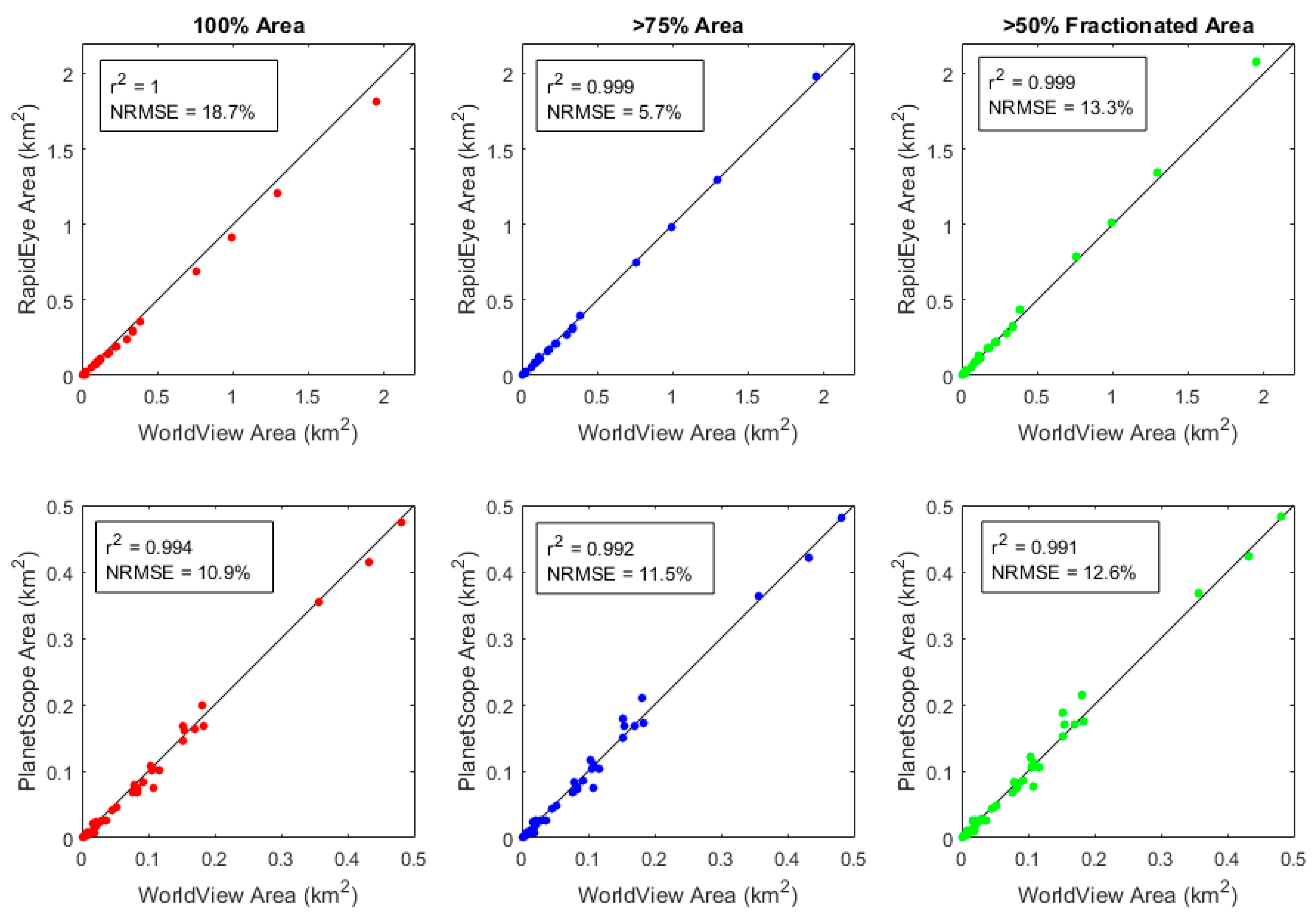
Figure 5.
Lake shorelines delineated from PlanetScope (blue), RapidEye (green) and WorldView (red) imagery. PlanetScope and RapidEye shorelines shown represent automated extraction of >75% water area. WorldView shorelines are manually delineated. Imagery © 2016, DigitalGlobe, Inc., Westminster, CO, USA.

Figure 6.
(a) Map of seven river reach segments and (b) time series of corresponding river effective width. Color and number of time series in (a) corresponds to color and number of reach in (b); (c) Time series of effective width for river reach #4 and corresponding Yukon River discharge at Eagle and (d) scatter between effective width and Yukon River discharge (Q) at Eagle The equation of the best fit curve in panel (d) (shown in red) is We = 10.9Q0.38 (R2 = 0.75).

Figure 7.
Changes in lake surface areas between (column 1, (a,d)) 23 June and 1 October, (column 2, (b,e)) 23 June and 17 August and (column 3, (c,f)) 17 August and 1 October. In the top row individual water bodies are represented as circles with the sizes of the circles scaled by the area of the change. Bottom row shows the pixel-based change in water fraction. Location of inset shown in top row. Red represents water loss, blue represents water gain.
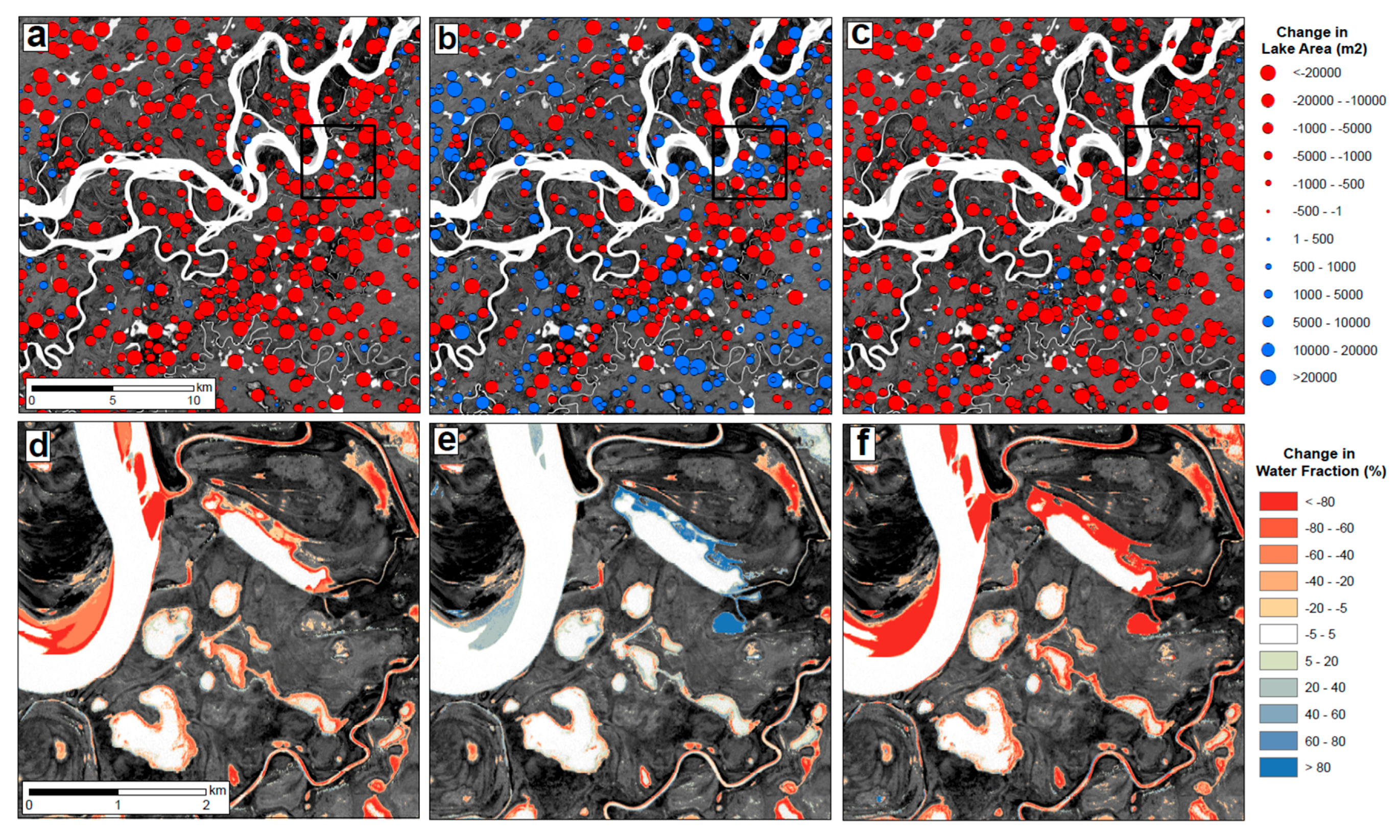
Figure 8.
Examples of lake area time series categorized as: (a) connected; (b) disconnected and (c) stable. The time series of lake area is shown on the right. Column 1 is NDWI imagery from 6/23 (observation 1), column 2 from 8/17 (observation 5), column 3 from 9/02 (observation 9) and column 4 from 10/01 (observation 12).

Figure 9.
Temporal correlation between Planet time series of lake surface area and Yukon River discharge reveal connected (green), disconnected (orange) and stable (light blue) lakes. Green dots are connected lakes (surface area standard deviation >10%, correlated to Yukon River discharge at p < 0.1), orange are disconnected (surface area std >10%, not correlated to Yukon River discharge) and light blue are stable (surface area std <10%).

Figure 10.
Normalized distribution of (a) top of atmosphere near infrared reflectance and (b) NDWI for Yukon Flats water bodies and surrounding vegetation in five different PlanetScope images. In the near infrared (a), water pixels are the left peak (lower band values) and in the NDWI (b), the second peak represents water pixels.
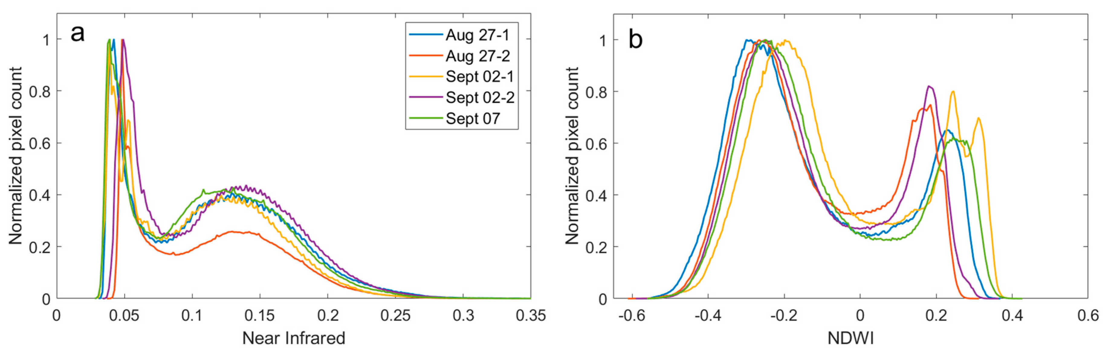
Figure 11.
(a) Geometric revisit time and (b) average time in days between cloud-free revisits for PlanetScope imagery north of 55°N when satellite constellation is at full operational capacity.
Figure 11.
(a) Geometric revisit time and (b) average time in days between cloud-free revisits for PlanetScope imagery north of 55°N when satellite constellation is at full operational capacity.
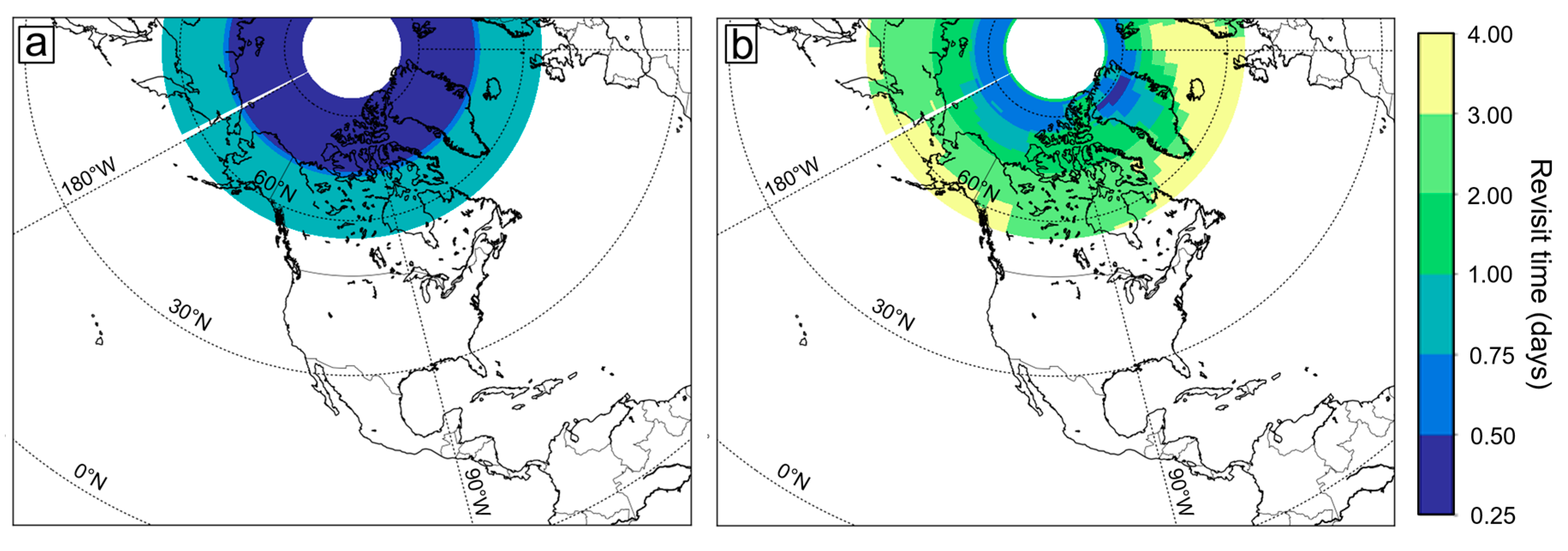
Figure 12.
Time series of river ice breakup on the Yukon shown in the near infrared band of PlanetScope imagery. Panels show (a) 2 May, (b) 6 May, (c) 7 May, (d) 12 May, (e) 12 May (7 min later) and (f) 15 May.
Figure 12.
Time series of river ice breakup on the Yukon shown in the near infrared band of PlanetScope imagery. Panels show (a) 2 May, (b) 6 May, (c) 7 May, (d) 12 May, (e) 12 May (7 min later) and (f) 15 May.


Table 1.
Specifications of the three satellite sensors operated by Planet. Information is correct as of date of publication.
Table 1.
Specifications of the three satellite sensors operated by Planet. Information is correct as of date of publication.
| Sensor | Number of Satellites | Bands | Spatial Resolution | Temporal Resolution |
|---|---|---|---|---|
| RapidEye | 5 | 5 (Blue, Green, Red, Far-Red, NIR) | 6.5 m | ~5.5 days |
| PlanetScope | ~170 | 4 (Blue, Green, Red, NIR) | 3.7 m | Daily |
| SkySat | 13 | 4 (Blue, Green, Red, NIR) | 0.8 m | Variable, with multiple opportunities per day |
Table 2.
List of images.
| Image ID | Sensor | Date | Observation |
|---|---|---|---|
| 20160623_220215_669714_RapidEye-4 | RapidEye | 23 June | 1 |
| 20160624_220552_669714_RapidEye-5 | RapidEye | 24 June | 2 |
| 20160725_215412_669714_RapidEye-3 | RapidEye | 25 July | 3 |
| 20160813_215232_669714_RapidEye-3 | RapidEye | 13 August | 4 |
| 222535_0669714_2016-08-16_0e0d | PlanetScope | 16 August | 5 |
| 20160817_220351_669714_RapidEye-2 | RapidEye | 17 August | 6 |
| 229647_0669714_2016-08-27_0e14 | PlanetScope | 27 August | 7 |
| 229821_0669714_2016-08-27_0e20 | PlanetScope | 27 August | 7 |
| 20160901_215044_669714_RapidEye-3 | RapidEye | 1 September | 8 |
| 232753_0669714_2016-09-02_0e19 | PlanetScope | 2 September | 9 |
| 232785_0669714_2016-09-02_0e30 | PlanetScope | 2 September | 9 |
| 20160907_215525_669714_RapidEye-4 | RapidEye | 7 September | 10 |
| 236414_0669714_2016-09-07_0e26 | PlanetScope | 7 September | 11 |
| 20161001_215759_669714_RapidEye-4 | RapidEye | 1 October | 12 |
| 234040_0669715_2016-09-02_0e0e | PlanetScope | 2 September | Validation |
| 234040_0669716_2016-09-02_0e0e | PlanetScope | 2 September | Validation |
| 238490_0669716_2016-09-02_0e26 | PlanetScope | 2 September | Validation |
| 20160908_215904_669817_RapidEye-5 | RapidEye | 8 September | Validation |
| 20160908_215905_669816_RapidEye-5 | RapidEye | 8 September | Validation |
| WV02_20160830213545_103001005A6E6600_16AUG30213545-P1BS | WorldView-2 | 30 August | Validation |
| WV03_20160908220049_1040010021B5F000_16SEP08220049-P1BS | WorldView-3 | 8 August | Validation |
| WV03_20160908220050_1040010021B5F000_16SEP08220050-P1BS | WorldView-3 | 8 August | Validation |
© 2017 by the authors. Licensee MDPI, Basel, Switzerland. This article is an open access article distributed under the terms and conditions of the Creative Commons Attribution (CC BY) license (http://creativecommons.org/licenses/by/4.0/).
Share and Cite
MDPI and ACS Style
Cooley, S.W.; Smith, L.C.; Stepan, L.; Mascaro, J. Tracking Dynamic Northern Surface Water Changes with High-Frequency Planet CubeSat Imagery. Remote Sens. 2017, 9, 1306. https://0-doi-org.brum.beds.ac.uk/10.3390/rs9121306
AMA Style
Cooley SW, Smith LC, Stepan L, Mascaro J. Tracking Dynamic Northern Surface Water Changes with High-Frequency Planet CubeSat Imagery. Remote Sensing. 2017; 9(12):1306. https://0-doi-org.brum.beds.ac.uk/10.3390/rs9121306
Chicago/Turabian StyleCooley, Sarah W., Laurence C. Smith, Leon Stepan, and Joseph Mascaro. 2017. "Tracking Dynamic Northern Surface Water Changes with High-Frequency Planet CubeSat Imagery" Remote Sensing 9, no. 12: 1306. https://0-doi-org.brum.beds.ac.uk/10.3390/rs9121306
Note that from the first issue of 2016, this journal uses article numbers instead of page numbers. See further details here.