UAV Remote Sensing Surveillance of a Mine Tailings Impoundment in Sub-Arctic Conditions


1
Water Resources and Environmental Engineering, University of Oulu, P.O. Box 4300, FI-90014 Oulu, Finland
2
Norut Northern Research Institute, P.O. Box 6434, NO-9294 Tromsø, Norway
*
Author to whom correspondence should be addressed.
Remote Sens. 2017, 9(12), 1318; https://0-doi-org.brum.beds.ac.uk/10.3390/rs9121318
Submission received: 22 November 2017
/
Revised: 12 December 2017
/
Accepted: 12 December 2017
/
Published: 15 December 2017
(This article belongs to the Special Issue The Use of UAVs in the Raw Material Sector, from Mineral Exploration to Post-Mining Monitoring)
Abstract
:Mining typically involves extensive areas where environmental monitoring is spatially sporadic. New remote sensing techniques and platforms such as Structure from Motion (SfM) and unmanned aerial vehicles (UAVs) may offer one solution for more comprehensive and spatially continuous measurements. We conducted UAV campaigns in three consecutive summers (2015–2017) at a sub-Arctic mining site where production was temporarily suspended. The aim was to monitor a 0.5 km2 tailings impoundment and measure potential subsidence of tailings. SfM photogrammetry was used to produce yearly topographical models of the tailings surface, which allowed the amount of surface displacement between years to be tracked. Ground checkpoints surveyed in stable areas of the impoundment were utilized in assessing the vertical accuracy of the models. Observed surface displacements were linked to a combination of erosion, tailings settlement, and possible compaction of the peat layer underlying the tailings. The accuracy obtained indicated that UAV-assisted monitoring of tailings impoundments is sufficiently accurate for supporting impoundment management operations and for tracking surface displacements in the decimeter range.

1. Introduction
Mining produces significant amounts of waste materials, and the volume of waste products is expected to increase in the future as lower grades of ores are utilized in mining [1,2]. One of the waste types produced is tailings, which comprise solid particles from mineral extraction and a mixture of water and additional components such as coagulants and flocculants. Tailings impoundments pose one of the most significant environmental risks in mining areas [2,3]. In particular, conventional storage of tailings in the form of a slurry can pose high environmental risks depending on the quality of tailings, due to potential water seepage, spills, and dam collapses. One option to reduce unwanted impacts on the surrounding environment is to store tailings in a drier format, using paste or cake techniques. Several authors discuss such techniques [4,5,6,7,8], the general principle of which is to decrease the water content of tailings using thickeners or filters. Dewatering changes the tailings continuum from a low-viscosity fluid to a more paste-like state. At the same time, it affects the behavior of the tailings, e.g., the consolidation rate (decrease in volume due to expulsion of water) and the stability of the tailings stack [5]. The paste technique is claimed to have numerous advantages compared with conventional slurry deposition, such as increased deposition angle, decreased land footprint, less frequent need to raise the embankments, fewer seepage and stability issues, and less segregated material [8,9]. However, research on the effects of cold climate conditions on paste storage is currently limited [2,10,11]. Moreover, deposition of tailings using the paste technique requires more investment and a higher degree of mine management compared with the conventional slurry storage approach [2,8].
Stringent regulations place high demands on proper design and management of tailings disposal procedures. Thus, long-term storage facilities could benefit from more effective monitoring methods during every step of the mine life cycle. Rico et al. [3] reviewed mine dam failures and noted that the most common cause of failure was meteorological events, such as extreme rain and snowmelt. The second most common cause was poor management. Freezing temperatures in cold climates, as in sub-Arctic or Arctic regions, can cause issues such as formation of permafrost within the impoundment. Permafrost can increase the strength of tailings while the matrix remains frozen, but upon thawing (e.g., due to climate change or particularly warm summers) it can have severe negative consequences for the stability, especially in the case of upstream embankment raising [10]. Another noteworthy problem is the high cost of maintenance of tailings dams after mine closure [3]. The behavior of tailings is very complex and can be affected by process modifications, flocculation, sedimentation, consolidation, segregation, deposition, freeze-thawing, and desiccation [12]. Therefore, use of modern remote sensing techniques to support conventional geotechnical measurements in the impoundment-scale monitoring of tailings could improve the management of tailings, and extend existing knowledge of tailings behavior.
Unmanned aerial vehicles (UAVs) can enable cost- and work-efficient surveillance of waste facilities [13,14,15,16]. UAVs and Structure from Motion (SfM) photogrammetry—a low-cost topographical survey technique developed from computer vision and conventional photogrammetry techniques—have gained popularity as a fast and flexible data acquisition system that can be used to produce orthomosaics and 3D models [13,14,15]. Recent reviews on UAVs and their utilization in topographical mapping are provided by Colomina and Molina [13] and Nex and Remondino [14]. UAV-SfM has recently been applied in mapping surface displacement in various fields, such as glaciology and landslide monitoring [17,18,19,20,21,22]. However, most mining-related research utilizing UAVs has focused on mapping open pit and stockpile geometry [23,24,25,26,27], and, to our knowledge, there is no published, peer-reviewed research addressing the utilization of UAVs in the context of mine tailings.
The main purpose of the present study was to determine the potential for utilizing UAVs in monitoring a tailings impoundment. Specific objectives were to monitor movements in the surface of the tailings deposit (e.g., due to settlement) and to gain a better understanding of using the UAV-SfM method in a sub-Arctic climate. Four field measurement campaigns using UAV platforms were performed to collect data, during September 2015 to August 2017. Global Navigation Satellite System (GNSS) measurements were performed to assess the accuracy of the UAV data. The SfM technique was used for producing orthomosaics, digital elevation models (DEMs), and point clouds. The settlement of tailings was estimated by generating DEMs of Difference (DoDs). The accuracy of the DEMs relative to GNSS measurements was assessed. Finally, the results and accuracy of the measurements, the limitations due to the sub-Arctic location of the study site, and the potential for utilizing UAVs in monitoring of tailings impoundments were considered.
2. Study Area
The study site, the Laiva mine, is located in central Finland, about 200 km south of the Arctic circle (Figure 1). Mining for gold and other metals started at the end of 2011 and was suspended in March 2014 due to low gold prices. The nearest weather station (Revonlahti, approximately 25 km to the north) indicates a 30 year (1981–2010) mean monthly temperature for the region of +15.9 °C in July and −9.3 °C in January, with the values staying below zero from November to March [28]. The area has snow cover for roughly six months of the year (November to April) and mean annual precipitation of 540 mm [28]. The presence of soil frost generally coincides with the cold and snowy months, with onset of frost around November, when the mean daily temperature drops below zero, and frost-free soil by mid-May, when the insulating snow cover has melted and air temperature stays above zero. In situ measurements indicate that soil frost can extend to 70 cm or deeper, depending on the soil texture and winter weather conditions (e.g., temperature, depth of snow cover).
The tailings impoundment is situated 6 kilometers from the processing plant, in the Vasaneva peatland. The current suspension of production at the mine provides an excellent opportunity to monitor changes in the tailings facility without the input of new material. The tailings impoundment area is approximately 0.5 km2 (length around 1 km, width around 0.5 km). The thickness of the tailings deposit varies across the impoundment, from a few meters up to around 10 m (average around 5 m). As the operation of the mine was short-lived prior to suspension of production, the overall size of the impoundment is small compared with typical tailings impoundments. The tailings in the facility are classified as sandy clayey silt (EN ISO) and the disposal method has varied over time from thickened to paste tailings, depending on the water content achieved in the thickening process. During active production, three main pumping stations were used inside the ring-dyke impoundment and the location of pumping alternated between these stations during operation.
3. Materials and Methods
3.1. UAV and Field Measurements
The four UAV field measurement campaigns were carried out in September 2015, July 2016, June 2017, and August 2017 (Table 1). The first campaign was conducted on 9 September 2015, using a Cryowing Scout fixed-wing UAV (produced by Norut, Tromsø, Norway) carrying a 12 megapixel (MP) Canon Powershot SX260 HS camera (Canon Inc., Tokyo Japan). The flight height was approximately 300 m and the average ground speed was ~20 m/s. A total of 664 photos were acquired, with ground resolution of about 10 cm/pixel, covering an area of about 2.8 km2 that included some of the surrounding forest and peatlands. The second campaign was conducted on 28 July 2016, using an Observer fixed-wing UAV (produced by Aranica AS, Tromsø, Norway) and an 18 MP Canon EOS M camera (Canon Inc., Tokyo, Japan) with a 22 mm lens (~35 mm full-frame equivalent). This time, the flight height was set at 150 m and the average ground speed was ~15 m/s. A total of 376 photos were acquired, with ground resolution of about 3 cm/pixel. During the 2015 and 2016 campaigns, a total of 12 (2015) and 15 (2016) ground control points (GCPs) were measured with a Topcon GR-5 RTK GNSS receiver (Topcon Positioning Systems Inc., Tokyo, Japan) (Figure 2). The GCPs were either painted or plastic/wooden targets installed on the surface.
During summer 2017, two UAV surveys were performed at the site: the first on June 6 and the second on August 8. These surveys used an Aerotekniikka M-017 fixed-wing UAV (produced by Maailmasta Oy, Oulu, Finland) and a professional-grade Sony Cyber-shot DSC-RX1R II (Sony Corporation, Tokyo, Japan) mirrorless camera with a 42 MP full-frame sensor and 35 mm fixed lens. The flight height for both surveys was approximately 150 m and the target flight speed was 14 m/s. During the June and August campaigns, 894 and 711 images were collected, respectively. The GCPs during the 2017 surveys were measured with a Satlab SLC multi-purpose RTK GNSS receiver (Satlab Geosolutions AB, Askim, Sweden). During the June campaign, 20 GCPs were collected (Figure 2). During the August campaign, 11 new GCPs were collected and eight existing sufficiently well-preserved GCPs were reused (from June 2017).
In addition to the UAV campaigns, field measurements were performed during 2016 to collect ground-truth data. A Trimble R8 RTK GNSS receiver (Trimble Inc., Sunnyvale, CA, USA) was utilized to collect 189 GNSS ground checkpoints in the service roads and dams surrounding the impoundment (Figure 2). These areas can be assumed to be relatively stable and, thus, the measurements can be used in estimating the quality of data produced with the SfM approach.
3.2. Data Processing
The photos from each campaign were processed using Agisoft Photoscan (Agisoft LLC, St. Petersburg, Russia), which employs an SfM photogrammetry technique to produce dense point clouds, digital elevation models (or more precisely, digital surface models), and orthomosaics. The SfM technique is described in detail by, e.g., Carrivick et al. [29] and Westoby et al. [30]. GCPs were used to improve orthorectification (Table 2). For one of the GCPs collected during 2016 and for one collected during August 2017, the distances between the input coordinates and the coordinates estimated from the images (i.e., the estimated orientation errors) were found to be an order of magnitude higher than for other points and they were discarded during the processing.
Co-registration of the different point cloud datasets was performed in CloudCompare [31] with manual adjustment and the inbuilt “fine registration” tool that utilizes the Iterative Closest Point (ICP) algorithm. The approach was (i) to create masks highlighting the presumably stable service road built on top of the embankment dam that surrounds the impoundment; and (ii) to utilize the corresponding point cloud segments in the fine registration. Easily recognizable topographical landmarks were first utilized in manual improvement of the horizontal co-registration, and then fine registration with ICP was used iteratively to find a better vertical co-registration. Finally, the iterated transformation matrices for the road segments were used in co-registration of the full datasets.
The June 2017 data was used as a baseline for co-registering the point clouds as well as the gathered 189 GNSS checkpoints. After co-registration, statistics on point-to-point differences between the point clouds were exported for further analysis. The point cloud datasets were converted to full resolution DEMs and the data quality was assessed by point-to-raster comparison with the GNSS ground checkpoints in ArcGIS 10.5 (Esri Inc., Redlands, CA, USA). Finally, 1 m/pix resolution raster DEMs were generated in order to simplify data visualization and smooth out outliers. DEMs of difference (DoD) highlighting the amount of ground displacement were generated in ArcGIS 10.5 by calculating the pixel-by-pixel elevation differences between individual elevation models:
where Zij,1 is the elevation of pixel ij during time t1, Zij,2 is the elevation of pixel ij during time t2, and t2 > t1.
ΔZij = Zij,1 − Zij,2
4. Results
4.1. Orthomosaics and Digital Elevation Models
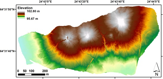
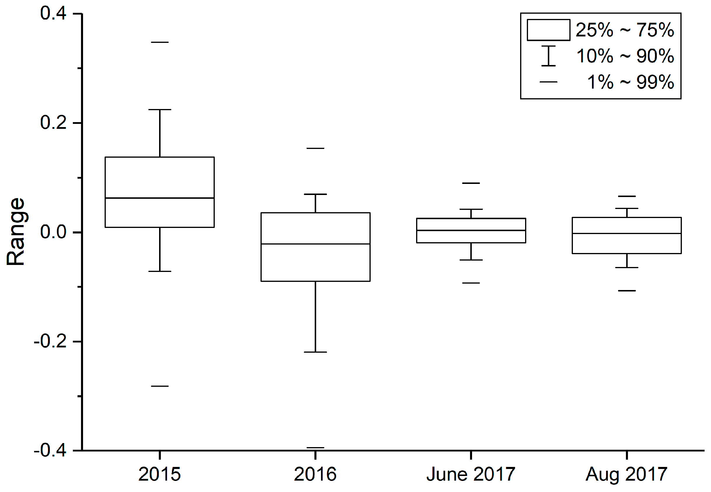
The first-level data products generated from the UAV campaigns were very high resolution orthophotos, dense point clouds, and raster DEMs (e.g., Figure 2 and Figure 3). The ground resolution achieved for the products generated improved from 2015 to 2016 and further to 2017, due to reduced flight height and improved camera quality. The improved ground resolution was accompanied by improved vertical accuracy, as indicated by comparison between the ground checkpoints and the corresponding DEM values highlighted in Table 3 and Figure 4. The mean errors presented in Table 3 give some indication of the global misalignments that remain after the data co-registration, whereas the mean absolute errors better highlight the internal accuracy of individual DEMs.
4.2. DEMs of Difference
DEMs of Difference (DoDs) between the September 2015 and June 2017 datasets (Figure 5A), and the June 2017 and August 2017 datasets (Figure 6A) were generated according to Equation (1). The 2016 dataset suffered from sub-optimal overlap among the aerial imagery surveyed. Although the dataset seemed quite accurate initially, even when compared against the GNSS ground checkpoints, it was eventually discovered to contain processing errors that manifested as easily distinguished banding in the DoDs generated. Thus, the 2016 dataset was discarded from the subsidence analysis.
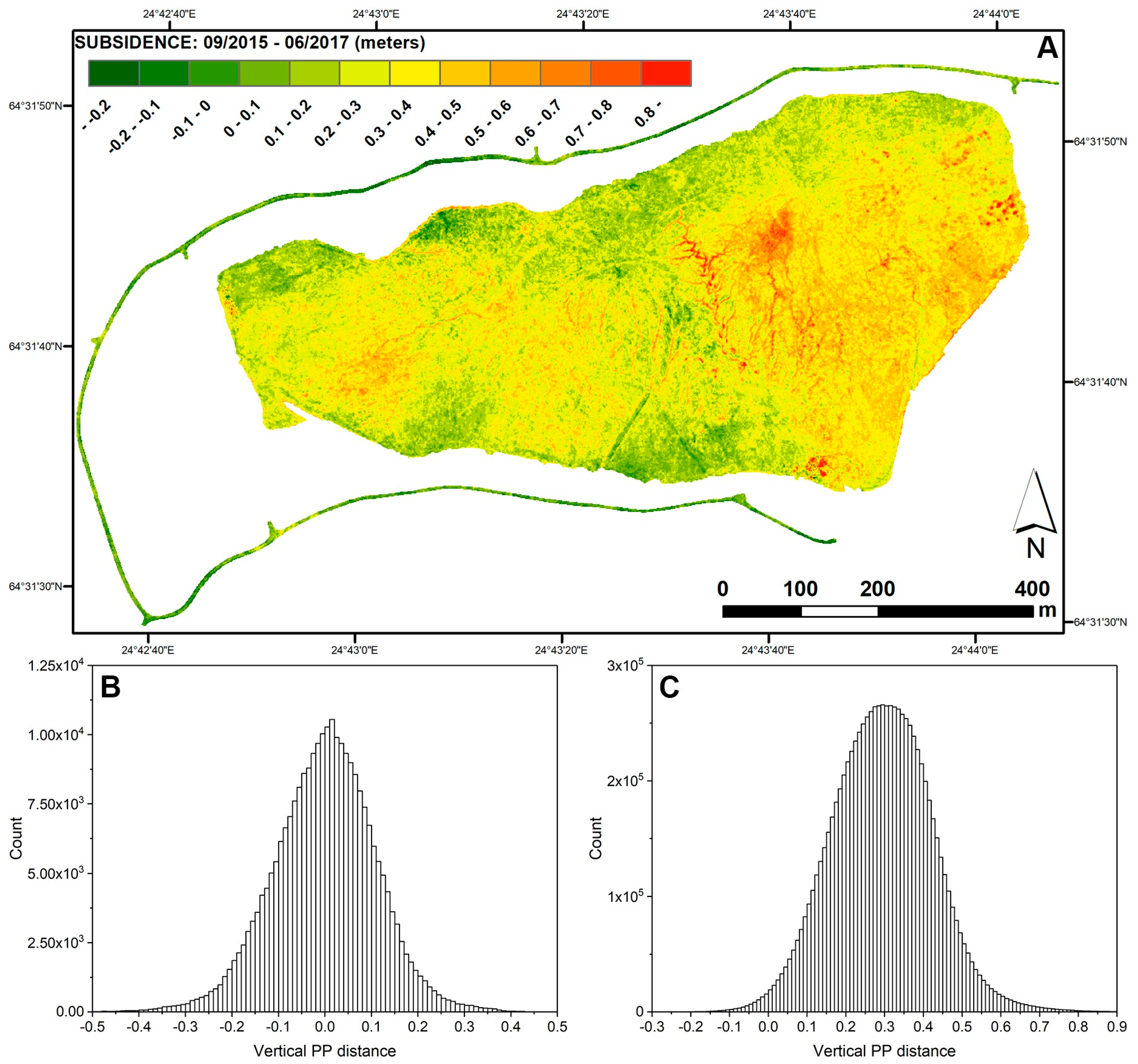
As mentioned, point-to-point distances between the point clouds were used for statistical analysis. The distribution of vertical point-to-point distances for the presumably stable service road in 2015–2017 is centered around zero change, with a mean of −0.001 m and median of 0.002 m (Figure 5B, Table 4). This was expected, since the road was used in co-registering the data. Analysis of the point-to-point distances indicated that the middle 99% of the values for the service road fell within the range −0.33 m to +0.31 m, giving some indication of data uncertainty. The distribution for the tailings surface (Figure 5C), on the other hand, centered around 0.29 m (mean 0.294 m, median 0.294 m), with the middle 99% of the values falling between −0.03 m and +0.68 m.
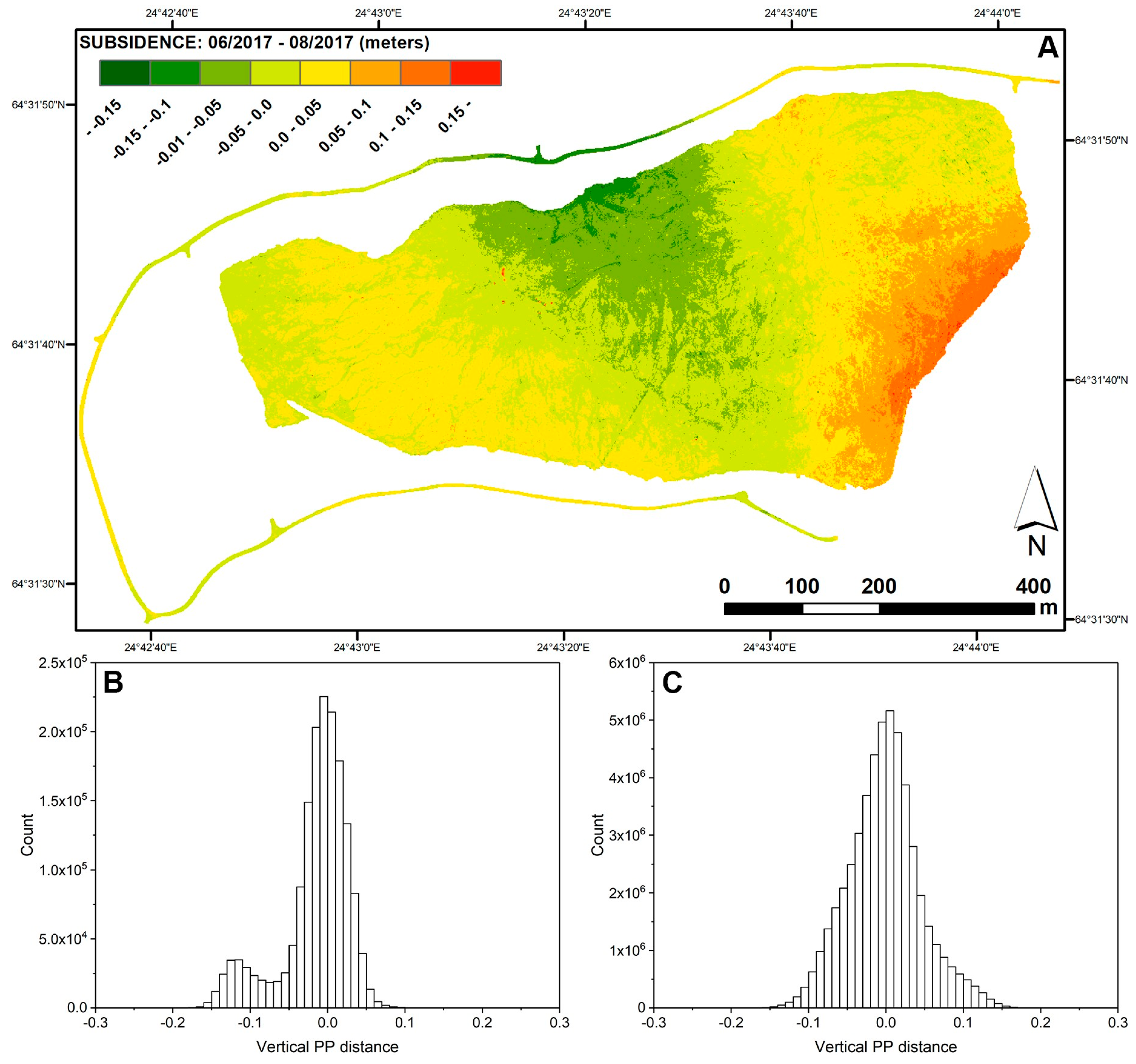
Between June 2017 and August 2017, the distribution of vertical point-to-point distances for the service road again peaked close to zero (mean −0.016 m, median −0.007 m) (Figure 6B). However, there was also a clear secondary peak around −0.12 m (Figure 6B). The middle 99% of the values were within the range −0.15 m to 0.06 m. The source of this secondary peak was clearly apparent in the northern part of the road DoD. Comparisons against the GNSS ground checkpoints measured along the service road (highlighted in Figure 2) indicated that in the June 2017 DEM there was an approximately −6 to −11 cm dip in values near the area and in the August 2017 DEM there was an approximately 2 to 7 cm bulge, which cumulatively resulted in the observed large negative anomaly in the calculated DoD.
The distribution of vertical point-to-point distances for the tailings surface in June 2017 to August 2017 is centered around zero (both mean and median −0.002 m), with the middle 99% of the values lying between −0.12 m and +0.13 m (Figure 6C). The negative anomaly in the northern part of the impoundment discussed in the above paragraph was reflected in the negative tail end of the distribution for the tailings surface. There was also a positive anomaly in the southeastern part of the tailings surface. Comparison against the GNSS ground checkpoints indicated an approximately 2 to 9 cm bulge in the June 2017 DEM and an approximately −2 to −10 cm dip in the August 2017 DEM near the southeastern area, thus cumulatively resulting in the positive anomaly observed.
5. Discussion
5.1. Results and Accuracy
The largest values of apparent subsidence (up to +80 cm in the 2015–2017 DoD; Figure 5A) seemed to be generally related to dendritic erosion patterns, small pools of water, and dead treetops. Some of the apparent subsidence might derive from true erosion, due to, e.g., precipitation and snowmelt, but it is probably related at least partly to the ability of the higher-resolution DEM for June 2017 (5 cm/pixel) to represent fine surface features more accurately than the lower-resolution DEM for 2015 (20 cm/pixel). Unfortunately, no ground truth data were available to validate the amount of tailings subsidence. However, it is noteworthy that the distribution of point-to-point distances for the presumably stable service road centered around ±0 cm change, whereas for the tailings surface the distribution shifted +30 cm towards subsidence in 2015–2017.
Considering the total thickness of the tailings deposit (up to ~10 m) and the time since the last deposition (2014), the values of apparent subsidence (up to +80 cm) seem somewhat high to be caused simply by tailings consolidation. However, the general trend in subsidence was at least in the expected direction and values closer to the distribution peak around +30 cm are more easily explained by tailings consolidation and settlement. It should also be noted that the tailings were deposited on top of a natural peat layer at least 1 m thick that can also undergo compaction. Peat soil is strongly compressible under load and it can continue to settle for a considerable time, thus causing some of the measured subsidence. The subsidence could also be affected by groundwater fluctuations and repeated freeze-thaw cycles which, depending on winter conditions, can affect at least the top ~70 cm of the tailings. Freezing and thawing are known to compact soil materials and to increase the rate of consolidation [11]. The subsidence detected appeared to be less severe along the edges of the impoundment. This might be due to some degree to data uncertainty, as is evident in the distribution of vertical point-to-point distances for the service road (Figure 5B). It might also be partly related to initially lower thickness of the tailings deposit, and consequently lower potential for consolidation-related settlement of the tailings and less compression of the underlying peat. An additional cause might be migration of materials from the middle of the impoundment towards the lower elevation edges, due to creep and/or, e.g., wind, rain, and snowmelt-related erosion.
Little to no observable change was expected between the June 2017 and August 2017 measuring campaigns, as the period between the surveys was short and the rate of consolidation is likely to have declined significantly since the end of tailings deposition in March 2014. Thus, the DoD for the 2017 datasets should give some indication of data reproducibility, as the gear and flight parameters used remained constant between the campaigns. With regards to uncertainty, the standard deviations for the 2017 road and tailings DoDs were 4.4 cm and 4.7 cm, respectively, which is greatly reduced from the 11.0 cm standard deviation obtained for the 2015–2017 road dataset. In a previous study, Clapuyet et al. [32] concluded that, all parameters being equal, the reproducibility of topographical UAV-based SfM measurements is very high and that the main limiting factor with regard to accuracy is the GNSS system used in surveying the georeferencing targets. The manufacturers report the accuracy of the RTK GNSS devices used in the present study to be generally around a few centimeters. Thus, the accuracy of the final models in our case was somewhat lower than the presumed GCP accuracy.
Numerous recent studies have focused on the accuracy, reproducibility, and optimization of UAV surveys utilizing SfM in variable locations [32,33,34,35,36,37,38,39] and can provide some insights. The accuracy is generally considered to be affected by various parameters, including camera parameters (e.g., focal length, sensor resolution, and exposure time), acquisition parameters (e.g., flight height and ground control network), environmental parameters (e.g., solar illumination and weather), and processing settings [40]. Also, the characteristics of the UAV (e.g., stability, velocity) can have an influence on the accuracy. It is important to note that different validation studies focus on slightly different aspects of accuracy and precision, and also utilize different types of validation methods [29]. Validation studies utilizing point-to-raster comparison (as was the case in this study with the 189 ground checkpoints) generally seem to provide much higher root-mean-square errors (RMSEs) than raster-to-raster or point-to-point comparison [29]. Furthermore, based on 50 validation studies, Carrivick et al. [29] demonstrated a clear increase in RMSE as the survey range and area increases.
Agüera-Vega et al. [33] conducted an accuracy assessment with variable terrain morphologies, flight heights, and GCP configurations. The number of GCPs clearly influenced the horizontal accuracy, with an increased number providing improved accuracy [33]. The vertical accuracy was not influenced by terrain morphology, while both flight height and number of GCPs had a significant influence on the RMSE of the vertical component, with lower flight heights giving higher accuracy [33]. Clapuyet et al. [32] reported that increasing the number of GCPs beyond a certain (area-dependent) number provided only negligible improvements in vertical accuracy. Tonkin and Midgley [35] showed that increasing the number of GCPs beyond a certain number can even increase the vertical RMSE if the positional accuracy of the survey equipment is variable, and highlighted the importance of a uniform spatial distribution of GCPs if highly accurate data are required.
In both of our 2017 surveys, the GCPs near the middle northern portion of the service road were the least accurate points reported by Agisoft Photoscan during processing. Some of the strongest inaccuracies in the final models were also detected in this area when compared against GNSS ground checkpoints. The origin of the inaccuracies in the southeastern corner, on the other hand, was not clearly apparent in the processing report. Increasing the number of GCPs could have improved the accuracy although, as indicated by the literature, would not always do so. With further processing, one remedy could be to try different combinations of GCPs to find the best fit to the ground checkpoints and also otherwise optimize the processing parameters [38].
A further practicality is the flight height, which affects the resolution, flight time, and processing requirements. In the case of a >1 km2 survey area (as in this study), a minimum flight height of 150 m is recommended in order to avoid extremely large datasets and long processing times while providing sufficient coverage [29]. Furthermore, local UAV regulations should be considered. For example, in Finland, exceeding the flight height of 150 m with a UAV requires a permit from the Finnish Transport Safety Agency. Improved camera quality (in 2017) clearly affected the data accuracy, as shown in Figure 4. A similar effect has been reported by, e.g., Mosbrucker et al. [39], who found that improving the information capacity of the camera system (12 megapixel, 380 mm2 sensor replaced by 36 megapixel, 860 mm2 sensor) increased the pixel matching quality, resulting in eightfold greater point density, sixfold greater accuracy, and 50% better precision. Further regression analysis of 67 datasets and related survey metrics from 16 validation studies indicated that photographic scale is the best explanatory variable to predict the accuracy of SfM data [39].
Another uncertainty in the present case was the stability of the service road, since there is no definitive certainty that the road has remained stable over the years. However, it is reasonable to assume that the road is among the most stable portions of the structure, considering that it is built on top of glacial till instead of peat and that stabilization work is typically performed in order to ensure stability under vehicle and machinery traffic. The same applies for the outer dams of the impoundment, which were utilized in surveying some of the ground checkpoints. As the road was utilized in co-registration of the datasets, it is at least possible to conclude that the tailings surface has moved relative to the road.
5.2. Application of UAVs for Monitoring Tailings Inpoundments
Tailings storage facilities can cover vast areas and thus require a comprehensive and widespread environmental monitoring system. Each impoundment is unique, tailor-made, and designed. Furthermore, the safety of the impoundment must be ensured by economically feasible means. Overall, the management of tailings impoundments needs several measurement methods for different monitoring purposes. The results from our case indicate that UAVs could be useful, fast, and cost-effective in monitoring the movement of paste tailings in the decimeter range. In the active mine phase, it is economically important to monitor the tailings storage volume in the impoundment and to optimize the disposal technique. The UAV-SfM method can be a useful tool for (i) mapping a tailings surface profile; (ii) calculating impoundment storage capacity; and (iii) predicting future needs more specifically, e.g., the need to raise surrounding dams or other maintenance work. From a geotechnical perspective, the UAV-SfM method can help to optimize the disposal scheme, e.g., it can help decide where to pump the tailings in the impoundment in order to use the storage capacity as efficiently as possible and check the tailings surface slope. The method is suitable for monitoring changes in the tailings surface, but it does not ultimately explain the reason for the changes.
The potential use of the method in management of tailings impoundments is not limited to the active phase. Tailings impoundments have to be closed safely and normally a cover is built above the impoundment to protect and minimize environmental effects. After closure of a mine, regular monitoring with UAVs could help map long-term scale settlements and movements in the tailings impoundment(s). UAVs can also be used early in the design phase for mapping potential locations for a tailings impoundment.
Another key issue related to tailings impoundments is dam safety. While dam safety is governed by different laws, safety guidelines, and industry standards, further improvements are needed to avoid the environmental disasters that still occur [2,3]. Dam safety is a key issue around the world and better monitoring methods are needed. As mine tailings areas are vast, dams can be several kilometers in length, but the required accuracy in monitoring dams for possible movement is typically in the range of millimeters up to a few centimeters. Thus, the accuracy achieved in this study with the UAV-SfM method limits its potential use to monitor tailings dam safety. For remote sensing of tailings dams, it could therefore be more reasonable to focus on utilizing, e.g., satellite-based differential radar interferometry, which can detect displacements in the millimeter range, although the spatial resolution is generally much lower (meters to tens of meters) [41,42].
Use of the UAV-SfM method in the field also has some limitations. For example, in sub-Arctic conditions, the time window for measurements is restricted. Snow cover obscures the surface visibility and the tailings surface can be covered with snow for many days per year (around six months at the study site). This means that the UAV-SfM method cannot replace other monitoring activities during wintertime. Heavy precipitation and snowmelt water cover can also prevent or limit UAV measurements. Furthermore, possible problems that can go unnoticed until data processing (e.g., inaccurate or too scarce GCPs) should be considered when working in areas to which access is restricted. One option would be to produce a low-quality model in the field and make supplementary measurements when needed. For the method to be applied in regular maintenance operations and UAV-supported monitoring by mine staff or authorities, the workflow and processing could be streamlined, e.g., in regular operation it would be practical to use fixed and accurately measured GCPs, and the flight, camera, and processing parameters could be optimized over time through experience. Thus, a greater focus on quality control and quality assurance (QA/QC) could help standardize the use of UAVs in monitoring mine environments.
6. Conclusions
UAVs and SfM-generated digital elevation models were utilized in monitoring a tailings impoundment and movement of the tailings surface during three consecutive summers (2015–2017). Point-to-raster comparisons between the DEMs produced and ground checkpoints indicated that vertical mean absolute error clearly decreased from 2015 (10.8 cm) to 2017 (2.8–3.5 cm), mainly owing to improved ground resolution (camera quality and flight height) and an increased number of GCPs. Utilization of stable areas such as service roads in data co-registration proved to be a suitable method for fine registration and mapping of relative changes.
The largest apparent subsidence values (+80 cm) in the 2015–2017 subsidence map produced seemed to be linked partly to erosional features, indicating actual erosion, and partly to differences in resolution between the datasets. The observed general trend in subsidence (mean 29.4 cm) was probably related to tailings settlement and compaction of the underlying peat layer. Data uncertainty for the 2015–2017 DoD as indicated by standard deviation was around ±11 cm, strongly reflecting the lower resolution and accuracy obtained during 2015. The two measuring campaigns performed during 2017 showed that by improving camera and ground control network quality, and generally using fixed settings and gear, it was possible to reduce the DoD standard deviation down to the ±5 cm range. The accuracy obtained for the DEMs and DoDs indicates that UAV-assisted monitoring of tailings impoundments is sufficiently accurate for management operations such as volume calculations and tracking surface movement in the decimeter range.
Acknowledgments
This study was funded by the Interreg Nord 2014–2020 program, Lapin Liitto, and Troms Fylkeskommune. It is also supported by K.H. Renlund Foundation, Tauno Tönning Foundation, and Maa- ja vesitekniikan tuki ry. We appreciate the help of the Norut UAV group: Rune Storvold, Stian Solbø, André Kjellstrup; the field crew who helped with data collection; and Mitta Oy and Jukka Tienhaara (Maailmasta Oy), who were responsible for UAV surveys during 2017.
Author Contributions
All authors conceived and designed the experiments; A.R. and C.D. performed the experiments and analyzed the data; A.R. and A.T. drafted the manuscript with help and comments from C.D. and P.M.R.; P.M.R. was the project leader.
Conflicts of Interest
The authors declare no conflict of interest. The sponsors played no role in the design of the study; in the collection, analysis, and interpretation of data; in the writing of the manuscript; and in the decision to publish the results.
References
- European Commission. Reference Document on Best Available Techniques for Management of Tailings and Waste-Rock in Mining Activities; European Commission: Brussels, Belgium, 2009; 557p. [Google Scholar]
- Wang, C.; Harbottle, D.; Liu, Q.; Xu, Z. Current state of fine mineral tailings treatment: A critical review on theory and practice. Miner. Eng. 2014, 58, 113–131. [Google Scholar] [CrossRef]
- Rico, M.; Benito, G.; Salgueiro, A.R.; Díez-Herrero, A.; Pereira, H.G. Reported tailings dam failures. A review of the European incidents in the worldwide context. J. Hazard. Mater. 2008, 152, 846–852. [Google Scholar] [CrossRef] [PubMed]
- Nguyen, Q.D.; Boger, D.V. Application of rheology to solving tailings disposal problems. Int. J. Miner. Process. 1998, 54, 217–233. [Google Scholar] [CrossRef]
- Kwak, M.; James, D.F.; Klein, K.A. Flow behaviour of tailings paste for surface disposal. Int. J. Miner. Process. 2005, 77, 139–153. [Google Scholar] [CrossRef]
- Henriquez, J.; Simms, P. Dynamic imaging and modelling of multilayer deposition of gold paste tailings. Miner. Eng. 2009, 22, 128–139. [Google Scholar] [CrossRef]
- Edraki, M.; Baumgartl, T.; Manlapig, E.; Bradshaw, D.; Franks, D.M.; Moran, C.J. Designing mine tailings for better environmental, social and economic outcomes: A review of alternative approaches. J. Clean. Prod. 2014, 84, 411–420. [Google Scholar] [CrossRef]
- Jewell, R.J.; Fourie, A.B. Paste and Thickened Tailings—A Guide, 3rd ed.; Australian Centre for Geomechanics: Perth, Australia, 2015; 356p. [Google Scholar]
- Tacey, W.; Ruse, B. Making tailings disposal sustainable; a key business issue. In Paste and Thickened Tailings—A Guide, 2nd ed.; Jewell, R.J., Fourie, A.B., Eds.; Australian Centre for Geomechanics: Perth, Australia, 2006; pp. 13–22. [Google Scholar]
- Alakangas, L.; Dagli, D.; Knutsson, S. Literature Review on Potential Geochemical and Geotechnical Effects of Adopting Paste Technology under Cold Climate Conditions; Luleå Tekniska Universitet: Luleå, Sweden, 2013; 36p. [Google Scholar]
- Knutsson, R.; Viklander, P.; Knutsson, S. Stability considerations for thickened tailings due to freezing and thawing. In Proceedings of the Paste 2016—19th International Seminar on Paste and Thickened Tailings, Santiago, Chile, 5–8 July 2016. [Google Scholar]
- Ahmed, S.I.; Siddiqua, S. A review on consolidation behavior of tailings. Int. J. Geotech. Eng. 2014, 8, 102–111. [Google Scholar] [CrossRef]
- Colomina, I.; Molina, P. Unmanned aerial systems for photogrammetry and remote sensing: A review. ISPRS J. Photogramm. Remote Sens. 2014, 92, 79–97. [Google Scholar] [CrossRef]
- Nex, F.; Remondino, F. UAV for 3D mapping applications: A review. Appl. Geomat. 2014, 6, 1–15. [Google Scholar] [CrossRef]
- Pajares, G. Overview and current status of remote sensing applications based on Unmanned Aerial Vehicles (UAVs). Photogramm. Eng. Remote Sens. 2015, 81, 281–329. [Google Scholar] [CrossRef]
- Allemand, P.; Delacourt, C.; Grandjean, P. Potential and limitation of UAV for monitoring subsidence in municipal landfills. Int. J. Environ. Technol. Manag. 2014, 17, 1–13. [Google Scholar] [CrossRef]
- Pierzchała, M.; Talbot, B.; Astrup, R. Estimating soil displacement from timber extraction trails in steep terrain: Application of an unmanned aircraft for 3D modelling. Forests 2014, 5, 1212–1223. [Google Scholar] [CrossRef]
- Turner, D.; Lucieer, A.; de Jong, S.M. Time series analysis of landslide dynamics using an Unmanned Aerial Vehicle (UAV). Remote Sens. 2015, 7, 1736–1757. [Google Scholar] [CrossRef]
- Bhardwaj, A.; Sam, L.; Martín-Torres, F.J.; Kumar, R. UAVs as remote sensing platform in glaciology: Present applications and future prospects. Remote Sens. Environ. 2016, 175, 196–204. [Google Scholar] [CrossRef]
- Fernández, T.; Pérez, J.; Cardenal, J.; Gómez, J.; Colomo, C.; Delgado, J. Analysis of landslide evolution affecting olive groves using UAV and photogrammetric techniques. Remote Sens. 2016, 8, 837. [Google Scholar] [CrossRef]
- Cook, K.L. An evaluation of the effectiveness of low-cost UAVs and structure from motion for geomorphic change detection. Geomorphology 2017, 278, 195–208. [Google Scholar] [CrossRef]
- Lizarazo, I.; Angulo, V.; Rodríguez, J. Automatic mapping of land surface elevation changes from UAV-based imagery UAV-based imagery. Int. J. Remote Sens. 2017, 38, 2603–2622. [Google Scholar] [CrossRef]
- Chen, J.; Li, K.; Chang, K.J.; Sofia, G.; Tarolli, P. Open-pit mining geomorphic feature characterisation. Int. J. Appl. Earth Obs. Geoinf. 2015, 42, 76–86. [Google Scholar] [CrossRef]
- Shahbazi, M.; Sohn, G.; Théau, J.; Menard, P. Development and evaluation of a UAV-photogrammetry system for precise 3D environmental modeling. Sensors 2015, 15, 27493–27524. [Google Scholar] [CrossRef] [PubMed]
- Tong, X.; Liu, X.; Chen, P.; Liu, S.; Luan, K.; Li, L.; Liu, S.; Liu, X.; Xie, H.; Jin, Y.; et al. Integration of UAV-based photogrammetry and terrestrial laser scanning for the three-dimensional mapping and monitoring of open-pit mine areas. Remote Sens. 2015, 7, 6635–6662. [Google Scholar] [CrossRef]
- Raeva, P.L.; Filipova, S.L.; Filipov, D.G. Volume computation of a stockpile—A study case comparing GPS and UAV measurements in an open pit quarry. Int. Arch. Photogramm. Remote Sens. Spat. Inf. Sci. 2016, 41, 999–1004. [Google Scholar] [CrossRef]
- Rossi, P.; Mancini, F.; Dubbini, M.; Mazzone, F.; Capra, A. Combining nadir and oblique UAV imagery to reconstruct quarry topography: Methodology and feasibility analysis. Eur. J. Remote Sens. 2017, 50, 211–221. [Google Scholar] [CrossRef]
- Pirinen, P.; Simola, H.; Aalto, J.; Kaukoranta, J.P.; Karlsson, P.; Ruujela, R. Reports 2012:1—Climatological Statistics of Finland 1981–2010; Finnish Meteorological Institute: Helsinki, Finland, 2012; 96p. [Google Scholar]
- Carrivick, J.L.; Smith, M.W.; Quincey, D.J. Structure from Motion in the Geosciences; Wiley-Blackwell: Oxford, UK, 2016; p. 208. [Google Scholar]
- Westoby, M.J.; Brasington, J.; Glasser, N.F.; Hambrey, M.J.; Reynolds, J.M. “Structure-from-Motion” photogrammetry: A low-cost, effective tool for geoscience applications. Geomorphology 2012, 179, 300–314. [Google Scholar] [CrossRef] [Green Version]
- CloudCompare (ver. 2.8.1) [GNU GPL Software]. Available online: http://www.cloudcompare.org/ (accessed on 28 August 2017).
- Clapuyt, F.; Vanacker, V.; Van Oost, K. Reproducibility of UAV-based earth topography reconstructions based on Structure-from-Motion algorithms. Geomorphology 2016, 260, 4–15. [Google Scholar] [CrossRef]
- Agüera-Vega, F.; Carvajal-Ramírez, F. Accuracy of digital surface models and orthophotos derived from Unmanned Aerial Vehicle Photogrammetry. J. Surv. 2016, 143, 04016025. [Google Scholar] [CrossRef]
- Jaud, M.; Passot, S.; Le Bivic, R.; Delacourt, C.; Grandjean, P.; Le Dantec, N. Assessing the accuracy of high resolution digital surface models computed by PhotoScan® and MicMac® in sub-optimal survey conditions. Remote Sens. 2016, 8, 465. [Google Scholar] [CrossRef]
- Tonkin, T.N.; Midgley, N.G. Ground-control networks for image based surface reconstruction: An investigation of optimum survey designs using UAV derived imagery and Structure-from-Motion Photogrammetry. Remote Sens. 2016, 8, 786. [Google Scholar] [CrossRef]
- Gillan, J.K.; Karl, J.W.; Elaksher, A.; Duniway, M.C. Fine-resolution repeat topographic surveying of dryland landscapes using UAS-based structure-from-motion photogrammetry: Assessing accuracy and precision against traditional ground-based erosion measurements. Remote Sens. 2017, 9, 437. [Google Scholar] [CrossRef]
- Gindraux, S.; Boesch, R.; Farinotti, D. Accuracy assessment of digital surface models from Unmanned Aerial Vehicles’ imagery on glaciers. Remote Sens. 2017, 9, 186. [Google Scholar] [CrossRef]
- James, M.R.; Robson, S.; d’Oleire-Oltmanns, S.; Niethammer, U. Optimising UAV topographic surveys processed with structure-from-motion: Ground control quality, quantity and bundle adjustment. Geomorphology 2017, 280, 51–66. [Google Scholar] [CrossRef]
- Mosbrucker, A.R.; Major, J.J.; Spicer, K.R.; Pitlick, J. Camera system considerations for geomorphic applications of SfM photogrammetry. Earth Surf. Process. Landf. 2017, 42, 969–986. [Google Scholar] [CrossRef]
- Slocum, R.K.; Parrish, C.E. Simulated imagery rendering workflow for UAS-based photogrammetric 3D reconstruction accuracy assessments. Remote Sens. 2017, 9, 396. [Google Scholar] [CrossRef]
- Di Martire, D.; Iglesias, R.; Monells, D.; Centolanza, G.; Sica, S.; Ramondini, M.; Pagano, L.; Mallorquí, J.J.; Calcaterra, D. Comparison between Differential SAR interferometry and ground measurements data in the displacement monitoring of the earth-dam of Conza della Campania (Italy). Remote Sens. Environ. 2014, 148, 58–69. [Google Scholar] [CrossRef]
- Necsoiu, M.; Walter, G.R. Detection of uranium mill tailings settlement using satellite-based radar interferometry. Eng. Geol. 2015, 197, 267–277. [Google Scholar] [CrossRef]
Figure 1.
Aerial image of the tailings storage area for the Laiva mine, its location in Finland (insert), the extent of the tailings impoundment surface, and the service road built on top of the embankment dam (which was used in the present analysis). Orthophoto courtesy of National Land Survey of Finland.

Figure 2.
Orthomosaic of the tailings impoundment for the Laiva mine generated from the images gathered during the 2015 survey. Different colored symbols indicate ground control points (GCPs) gathered during different campaigns. Purple crosses indicate the locations of the 189 ground checkpoints gathered in 2016 using a Trimble R8 RTK GNSS device.

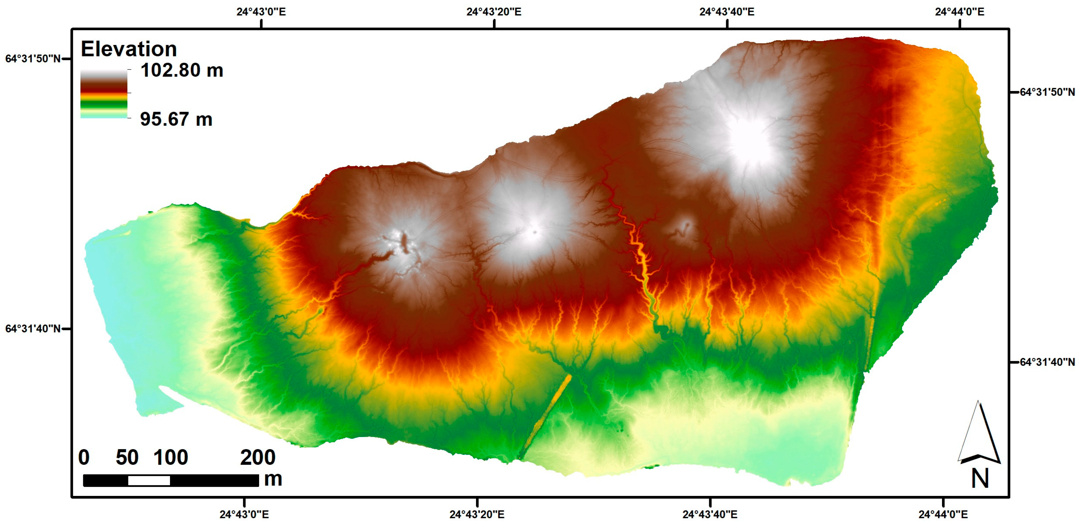
Figure 3.
Digital elevation model of the tailings surface produced from the images gathered during the June 2017 survey.
Figure 3.
Digital elevation model of the tailings surface produced from the images gathered during the June 2017 survey.

Figure 4.
Box plots highlighting the range of differences between the elevations of ground checkpoints and the corresponding values in the digital elevation maps (DEMs) generated. The middle line and boxes indicate the median and middle 50% of values, respectively. The whiskers indicate the 10–90% range of values, and the outer dashes indicate the 1–99% range of values.

Figure 5.
(A) Observed subsidence of the tailings surface between September 2015 and June 2017, (B) distribution of point-to-point (PP) elevation differences in the service road, and (C) distribution of point-to-point elevation differences in the tailings surface between the 2015 and 2017 point clouds.

Figure 6.
(A) Apparent subsidence between the June 2017 and August 2017 surveys, (B) distribution of point-to-point (PP) elevation differences in the service road, and (C) distribution of point-to-point elevation differences in the tailings surface between the June 2017 and August 2017 point clouds.


Table 1.
Field measurement campaigns, utilized equipment, and key parameters. The focal length is given as full-frame equivalent length. GNNS refers to the Global Navigation Satellite System receiver utilized in surveying the ground control points (GCPs).
Table 1.
Field measurement campaigns, utilized equipment, and key parameters. The focal length is given as full-frame equivalent length. GNNS refers to the Global Navigation Satellite System receiver utilized in surveying the ground control points (GCPs).
| 2015 | 2016 | June 2017 | August 2017 | |
|---|---|---|---|---|
| Date | 9 September 2015 | 28 July 2016 | 6 June 2017 | 8 August 2017 |
| Camera | Canon SX260 | Canon EOS M | Sony RX1R II | Sony RX1R II |
| Resolution | 12 MP | 18 MP | 42 MP | 42 MP |
| Focal length | 25 mm | 35 mm | 35 mm | 35 mm |
| Images | 664 | 376 | 894 | 711 |
| Flight height | 300 m | 150 m | 150 m | 150 m |
| Overlap | ~80/80 | ~40/40 1 | ~75/75 | ~75/75 |
| Covered area | ~2.8 km2 | ~1 km2 | ~1 km2 | ~1 km2 |
| GNSS | Topcon GR-5 | Topcon GR-5 | Satlab SLC | Satlab SLC |
| GCPs | 12 | 15 | 20 | 19 |
1 The aim was 80/80 overlap which was missed due to a calculation error.
Table 2.
Number of ground control points (GCPs) utilized in orthorectification for different datasets and the horizontal (XY), vertical (Z), and total orientation errors (root mean square errors) reported by Agisoft Photoscan during data processing.
Table 2.
Number of ground control points (GCPs) utilized in orthorectification for different datasets and the horizontal (XY), vertical (Z), and total orientation errors (root mean square errors) reported by Agisoft Photoscan during data processing.
| 2015 | 2016 | June 2017 | August 2017 | |
|---|---|---|---|---|
| GCPs | 12 | 14 | 20 | 18 |
| XY (cm) | 2.638 | 3.654 | 1.744 | 1.267 |
| Z (cm) | 0.345 | 0.838 | 2.065 | 1.457 |
| Total (cm) | 2.050 | 3.749 | 2.463 | 1.785 |
Table 3.
Ground pixel resolution (RES) of the orthomosaic and DEM datasets produced, and the mean error (ME), mean absolute error (MAE), root mean square error (RMSE), and standard deviation (STDEV) of the DEM vertical values when compared against ground checkpoints.
Table 3.
Ground pixel resolution (RES) of the orthomosaic and DEM datasets produced, and the mean error (ME), mean absolute error (MAE), root mean square error (RMSE), and standard deviation (STDEV) of the DEM vertical values when compared against ground checkpoints.
| 2015 | 2016 | June 2017 | August 2017 | |
|---|---|---|---|---|
| Ortho RES | 10 cm/pix | 3 cm/pix | 2 cm/pix | 2 cm/pix |
| DEM RES | 20 cm/pix | 6 cm/pix | 5 cm/pix | 5 cm/pix |
| DEM ME | 7.0 cm | −4.4 cm | 0.0 cm | −0.7 cm |
| DEM MAE | 10.8 cm | 8.5 cm | 2.8 cm | 3.5 cm |
| DEM RMSE | 13.8 cm | 12.2 cm | 3.6 cm | 4.2 cm |
| DEM STDEV | 11.9 cm | 11.4 cm | 3.6 cm | 4.2 cm |
Table 4.
Mean, standard deviation (STDEV), mean absolute deviation (MAD), 1st and 3rd quartiles (Q1, Q3), and 0.5th and 99.5th percentiles (P0.5, P99.5) for the vertical point-to-point distributions.
Table 4.
Mean, standard deviation (STDEV), mean absolute deviation (MAD), 1st and 3rd quartiles (Q1, Q3), and 0.5th and 99.5th percentiles (P0.5, P99.5) for the vertical point-to-point distributions.
| September 2015–June 2017 Road | September 2015–June 2017 Tailings | June 2017–August 2017 Road | June 2017–August 2017 Tailings | |
|---|---|---|---|---|
| Mean | −0.1 cm | 29.4 cm | −1.6 cm | −0.2 cm |
| STDEV | 11.0 cm | 12.9 cm | 4.4 cm | 4.7 cm |
| MAD | 8.6 cm | 10.2 cm | 3.2 cm | 3.6 cm |
| Q1 | −0.7 cm | 20.7 cm | −2.8 cm | −3.2 cm |
| Q3 | 0.7 cm | 37.9 cm | 1.2 cm | 2.4 cm |
| P0.5 | −32.8 cm | −2.9 cm | −14.7 cm | −11.6 cm |
| P99.5 | 30.6 cm | 67.7 cm | 6.0 cm | 13.1 cm |
© 2017 by the authors. Licensee MDPI, Basel, Switzerland. This article is an open access article distributed under the terms and conditions of the Creative Commons Attribution (CC BY) license (http://creativecommons.org/licenses/by/4.0/).
Share and Cite
MDPI and ACS Style
Rauhala, A.; Tuomela, A.; Davids, C.; Rossi, P.M. UAV Remote Sensing Surveillance of a Mine Tailings Impoundment in Sub-Arctic Conditions. Remote Sens. 2017, 9, 1318. https://0-doi-org.brum.beds.ac.uk/10.3390/rs9121318
AMA Style
Rauhala A, Tuomela A, Davids C, Rossi PM. UAV Remote Sensing Surveillance of a Mine Tailings Impoundment in Sub-Arctic Conditions. Remote Sensing. 2017; 9(12):1318. https://0-doi-org.brum.beds.ac.uk/10.3390/rs9121318
Chicago/Turabian StyleRauhala, Anssi, Anne Tuomela, Corine Davids, and Pekka M. Rossi. 2017. "UAV Remote Sensing Surveillance of a Mine Tailings Impoundment in Sub-Arctic Conditions" Remote Sensing 9, no. 12: 1318. https://0-doi-org.brum.beds.ac.uk/10.3390/rs9121318
Note that from the first issue of 2016, this journal uses article numbers instead of page numbers. See further details here.