GAN-Assisted Two-Stream Neural Network for High-Resolution Remote Sensing Image Classification


1
The State Key Laboratory of Information Engineering in Surveying, Mapping and Remote Sensing, Wuhan University, Wuhan 430079, China
2
Collaborative Innovation Center of Geospatial Technology, Wuhan University, Wuhan 430079, China
*
Author to whom correspondence should be addressed.
Remote Sens. 2017, 9(12), 1328; https://0-doi-org.brum.beds.ac.uk/10.3390/rs9121328
Submission received: 17 October 2017
/
Revised: 30 November 2017
/
Accepted: 16 December 2017
/
Published: 18 December 2017
(This article belongs to the Section Remote Sensing Image Processing)
Abstract
:Using deep learning to improve the capabilities of high-resolution satellite images has emerged recently as an important topic in automatic classification. Deep networks track hierarchical high-level features to identify objects; however, enhancing the classification accuracy from low-level features is often disregarded. We therefore proposed a two-stream deep-learning neural network strategy, with a main stream utilizing fine spatial-resolution panchromatic images to retain low-level information under a supervised residual network structure. An auxiliary line employed an unsupervised net to extract high-level abstract and discriminative features from multispectral images to supplement the spectral information in the main stream. Various feature extraction types from the neural network were selected and jointed in the novel net, as the combined high- and low-level features could provide a superior solution to image classification. In traditional convolutional neural networks, increased network depth might not influence the network performance perceptibly; however, we introduced a residual neural network to develop the expressive ability of the deeper net, increasing the role of net depth in feature extraction. To enhance feature robustness, we proposed a novel consolidation part in feature extraction. An adversarial net improved the feature extraction capabilities and aided digging the inherent and discriminative features from data, with increased extraction efficacy. Tests on satellite images indicated the high overall accuracy of our novel net, verifying that net depth or number of convolution kernels affected the classification capability. Various comparative tests proved the structural rationality for our two-stream structure.
1. Introduction
With the continuous development of earth observation, very high resolution (VHR) satellite imaging plays a significant role in various applications, including image classification, change detection, object recognition, land-cover mapping, building extraction and urban planning [1,2,3,4,5]. Aspects such as the rich patterns, ground features and geometrical information of VHR satellite image classification form the basis to these applications.
However, in per-pixel automatic classification, continuously increasing the resolution brings about clearer images and more detailed information; however, it also increases the intra-class variance and lowers the inter-class variance, which inevitably increases the difficulty of automatic classification [6]. Consequently, feature extraction methods that rely solely on spectral information can hardly achieve satisfactory classification results.
Consequently, the crux of classification is how to extract features from VHR satellite images effectively. Most traditional feature extraction methods originated from hand-engineered solutions [7,8,9,10] but feature designs and selections require human labor and prior knowledge and are mostly aim specific. Features designed for specific images and land features are difficult to be applied in automatic image classification. Moreover, the threshold determination makes the classification empirical; therefore, it cannot be used as a generalized method.
The appearance of deep learning (DL) has enabled discovering the inherent and potential features directly from the images and DL can extract the hierarchical features from the images. Low-level features from a shallow network represent details, whereas high-level features are more generic, abstract, discriminative and robust, usually determining what the objects are and remaining invariant to local changes. DL does not require artificial feature descriptor design and makes superior use of the features in the original data. Among all the deep learning models, the convolutional neural network (CNN) is considered an extremely successful model. It connects a node in the hidden layer only with a portion of the continuous input data, leading to a reduced number of connections and parameters, making the network easier to train [11]. The feature extractions by CNN are usually classified as supervised and unsupervised types. Supervised networks utilize labeled samples to adjust the extraction network parameters and classifiers constantly, with the extracted features being more specific. Unsupervised networks, such as Stacked Convolutional Auto Encoder (SCAE) [12], extract more general and robust features from the unlabeled data, retaining the essential aspects in the data. Both structures, i.e., CNN and SCAE, have merits and value; however, in general, CNN has achieved superior results in remote sensing image classification because of its characteristics [13,14,15,16].
It is believed that the expression ability of CNN would grow along with an increase in the network layer. However, under the normal convolution layer stack, the network performance growth might not be proportional to the network depth growth. In addition to the computational costs and the overfitting influences, the vanishing gradient could increase the difficulty of deep learning with the growth in network depth. However, if we assume that all the increased networks employed identity mapping, the increased network layers would not cause performance loss. Accordingly, low-level network training loss is the upper limit of its respective deep-level network and deep-level networks are at least equal to or surpass the shallow networks in expression ability [17]. Therefore, adding deep residual learning to CNN could be helpful in such situations. He et al. [18] constructed a 34-layer deep residual network employing the residual concept. This network was found superior to the VGG19 network and the 34-layer plain net, verifying its feasibility in the very-deep structure and its ability to solve the degradation problem. However, such residual CNN solutions are uncommon in VHR satellite image per-pixel classification.
In addition to adopting the appropriate feature extraction methods, acquiring more ground object information is another way to increase the feature extraction efficiency of the VHR satellite image. Panchromatic (PAN) and multispectral (MS) image fusion can be used for this purpose. Generally, PAN images have higher resolutions and the object edges are more discriminative, which could solve the ‘where is the object?’ problem. However, as the MS images contain richer spectral information, they could identify the ‘what is the object?’ problem much easier. Therefore, a combination of ‘where’ and ‘what’ could contribute to higher classification accuracy. For instance, Huang et al. [19] first fused PAN and MS images from the Chinese ZY-3 satellite, using various types of information indexes to classify the fusion images. Huang et al. [5] fused PAN and MS images of Vancouver and conducted full convolutional classification of PAN-sharpened RGB and NRG, subsequently fusing the classification results to extract buildings. Zhong et al. [20] enhanced MS image resolutions based on the super-resolution of the convolutional neural network, subsequently using the Gram–Schmidt transform process to fuse the MS and PAN images.
However, this type of fusion, with high-frequency detailed information, could lead to spectral distortion, which is not favorable to the subsequent interpretation and identification of ground objects. Hence, our study proposed a novel two-steam (main line and auxiliary line) deep neural network, based on PAN and MS image feature fusion for VHR remote sensing image-feature extraction and per-pixel classification.
Our method therefore differs from the methods mentioned above. In our study, the PAN image residual network was used as a main line for end-to-end and pixel-to-pixel classification and using the residual network to improve the expression ability of the deep network and to reduce the degradation problem. The edge and location features were retained because of the high spatial resolution characteristic in the full-resolution panchromatic image. Considering that the spectral information of an MS image was more suitable to determine the nature of a ground object, we used unsupervised MS image feature extraction as the auxiliary line. This utilized CNN and Stacked Convolutional Auto Encoder [12] to extract general, abstract and useful features. Such features retained the inherent and essential aspects in a robust and discriminative way in the data; therefore, being more suitable to determine what the objects were. The features extracted from the main and auxiliary lines were fused by layering in the residual network to combine various and abundant information from the different lines. This granted the network both ‘what’ and ‘where’ features that facilitated superior object identification and classification. In addition to the structure described above, we attempted to increase the quality of the features extracted by the network. For this purpose, we introduced the adversarial network concept to optimize the feature extraction ability of the network, making the extracted features more representative. Usually, we evaluate the effectiveness of the extracted features and optimized the feature extraction network by placing features directly into thee classifiers and assessing the classification results. However, with the appearance of the generative adversarial network (GAN) [21], we obtained a novel method to increase the feature extraction ability of the network. GAN is aimed at confusing the classifiers about whether the samples were generated by the generator or were the real ones. If successful, it verified that the extracted features were effective and powerful enough to simulate the real images. Radford et al. [22] conducted unsupervised representation learning by utilizing deep convolutional generative adversarial networks (DCGANs) and proved the efficiency of GAN. Luc et al. [23] first applied the GAN concept in image segmental classification, allowing the adversarial net to determine whether the segmentation results were generated or were the ground truth. In this respect, GAN obtained satisfactory results. We believe that we could use GAN to verify the effectiveness of the extracted features and, subsequently, to optimize the feature extraction network to enhance its feature extraction abilities.
The primary contributions of our study are as follows:
- We proposed a novel two-stream neural network to track low-level and high-level features simultaneously in order to enhance HR remote-sensing image classification. The data from different detectors were considered in this two-stream approach and, based on the respective characteristics of the data, this method integrated two different types of neural networks in a novel way. These are the supervised residual network and the unsupervised SCAE network, which were integrated to extract and combine features from different levels, contributing to final end-to-end and pixel-to-pixel classification.
- We rationally utilized the residual network to solve the performance impact of the deeper network that appeared in CNN, successfully developed the expressive ability of the deeper net and revealed that net depth could improve the classification accuracy notably.
- We introduced the concept of GAN, which is rare in HR remote sensing image classification. GAN helped to enhance the feature extraction ability of the network and contributed to exploring the inherent and most-discriminative features, enhancing the effectiveness of feature extraction.
The remaining parts of the article are organized as follows. Firstly, we briefly introduce the two-stream net related work in Section 2. In Section 3, the background knowledge of basis of our network has been explained. In Section 4, we introduce and elaborate on the proposed network, including the basic principles of the network components, as well as the training and classification methods. In Section 5 and Section 6, we describe the experiment-related contents, including the experimental data, an analysis of the experimental results and a discussion. Our conclusion is presented in Section 7.
2. Related Work
Feature extraction and fusion is an extremely common concept in remote sensing image segmentation and classification. Usually, ground object features are extracted with different methods or from different data sources and subsequently fused to obtain richer features. Such features represent the nature of the objects, enhancing the suitability to determine what these objects are.
Studies on using feature fusion to enhance VHR image segmentation and classification usually focus on fusing the features from the different layers. For example, Long et al. [24] not only used the last layer for upsampling but also used the features in the previous layers for fusion. The features in the first few layers had a relatively smaller receptive field and superior local feature presentations, whereas the features in the latter layers had a larger receptive field. This work obtained extremely satisfactory segmentation results after fusing the features from the different layers. Li et al. [25] used the same CNN to extract features from multiscale images, subsequently applied MIFK coding to features in the corresponding layer, unified the features from all the layers and finally reduced their dimensions to serve as the classifier input. These authors believe that the combined features from the different layers contain richer information. Ronneberger et al. [26] designed a U-Net to concatenate and localize high-resolution features in a contracting path and to upsample the features in the corresponding layers. The studies mentioned above have used mainly the merits of the hierarchical features in deep learning. The representation of a hierarchical feature is similar to how an image is formed. The points compose the edges, the edges compose the graphs, the graphs compose the parts and the parts compose the objects. However, all these features are from the same visualization of the objects to be classified but the extracted features from different levels of details are used to enrich the representation of the ground objects.
Accordingly, various studies have focused on the extraction of image features and fusion from diverse sources or image detectors. The same object could show the features of different levels of details, as well as the different features in images of different spectrums or from different sources. For example, Hu et al. [27] used multiple source images (hyperspectral images and polarimetric synthetic aperture radar (PolSAR) images) of the same area and subsequently extracted the features from two types of images with the two-stream convolutional neural network and finally fused the high-level features in the last layer. This method applied fusion at the feature level, which differs from the other methods [28,29] that unify the different image data or result data by different classifiers and subsequent average prediction scores. Huang et al. [5] applied convolution and deconvolution on the red, green, blue (RGB) and near-infrared, red green (NRG) band, respectively and subsequently fused the extraction result maps to obtain the final building extraction results. Although these networks adopted the two-stream structure, feature fusion only occurred in the highest level or the result layer. Such features had larger receptive fields and were more abstract; however, the influences of the low-level features on localization were omitted to some degree. To solve this problem, Pohlen et al. [17] utilized one full-resolution stream to keep boundary information and employed another stream to acquire abstract and robust features by process like pooling. The two streams were connected by layer so that the network possessed high-level and low-level features in the same time. Gao et al. [30] proposed to concatenate location prior information with features extracted from FCN-16s based two-stream network which is composed of feature extraction lines for RGB and contour maps. The added information helped network perform better in road detection. Nevertheless, most of two-stream networks mentioned above usually employ the same network structure configurations for different data sources. Although the network parameters of the two lines could begin to differ during network optimization, the feature characteristics extracted from the same or similar network structures tended to be similar and the two networks in the two different lines seldom interacted with each other. Therefore, it could be queried whether it would be beneficial to choose different networks for different data sources according to their own characteristics. Tao et al. [31] used two data sources with different classification methods during VHR image classification. They used a full convolutional network on the labeled VHR image data to be classified for classification training and an unsupervised network on the UC Merced dataset for the extraction of the unlabeled data feature. That study employed interactive training on the two-stream network and the feature-extraction parameters trained by the unsupervised network to improve constantly the convolution parameters of the full convolution network. This ensured that the extraction of the supervised network was constrained and supported by the unsupervised network. This method bypassed feature fusion and applied iterations directly to the network parameters; however, the two networks would extract features from the data sources of dramatically different contents. When significant differences were present in the feature natures of the data source, the parameters from the two networks could differ substantially. Using the parameters from the two streams for alternate iteration training could result in oscillation and could make it difficult for them to converge.
Informed by these research findings, we proposed an improved two-stream network for the feature extraction and classification of remote sensing images. Both PAN and MS images were used for the same area and different network structures were used for different data, tailored to their characteristics, which formed a two-stream network (main and auxiliary lines). On the main line, the residual network was applied to labeled PAN image patches for supervised feature extraction and classification training and the full resolution was maintained throughout the procedure. On the other line, unsupervised hierarchical feature extraction was used on MS image patches. We used the supervised network for PAN images because such images have VHRs and more discriminative edges, which are easy to label. Maintaining the full resolution enabled us to focus more on the low-level features, such as edge characteristic information and the like. The MS images had lower resolution compared with the PAN images and the boundaries between the ground objects were blurrier but the MS images had richer spectral information that enabled easier high-level feature extraction of ground objects and surrounding environments. This could be realized by the unsupervised network. There was no need to label all the pixels on the patches. We used hierarchical features from the MS data feature extraction network as support data and, for each feature layer, we fused the features with those from the corresponding layers in the main line. Subsequently, we used the results for the extraction of the next layer features of the main line. Feature fusion of the main and the auxiliary lines not only enabled the network focusing on features at different levels of details but also considered the different characteristics on images from the different sensors. Feature fusion by layer made the features richer in each layer and more suitable for extraction in the next layer. Furthermore, there were more interactions between the networks in the two lines during the feature fusion in each layer, which promoted the training of the two networks.
3. Background Knowledge
The proposed two-stream neural network involves several kinds of key components, such as Residual Network and Generative Adversarial Net mentioned in the introduction section. Nevertheless, no matter how complicated or advanced those technologies are, the basis, or the common ground for those skills is still convolutional neural network (CNN), a kind of method in deep learning (DL). So, in this background knowledge section, the brief introduction to DL and CNN will be presented for better understanding of our novel neural network.
DL is a kind of method simulating reaction of human brain when recognizing objects through multi-layer process from retina to cortex [32], which is designed to help extracting general, invariant and robust features.
Usually, a presentation of image is made of hierarchical features, to be more specific, points make up edges, edges make up graphs, graphs make up parts and parts make up objects. Consequently, DL can be utilized to get hierarchical features and employ lower level features to generate higher ones.
CNN is a kind of DL method. It is composed of several building blocks, each of them serves as a feature extraction stage, to extract hierarchical features. Building blocks from lower layer extract low level features, especially detailed information, while latter blocks try to preserve high level features, coarse but abstract and general. Each building block is formed of convolution layer, non-linearity layer and pooling layer. But the last one is not always required and is up to the actual situation.
The convolution layer utilizes kernels to operate convolution, in other words, weighted stack on the corresponding portion of the input data. This layer simulates the characteristics of neural network in which certain section in human brain’s visual cortex will correspond to a local area. So, convolution operation will connect one hidden layer node only with part of consecutive data from last layer, which decreases connection and the number of parameters, to make it easy to train [11]. The kernel size determines the size of receptive field while the third dimension of the kernel stands for the number of output feature maps. The more feature maps, the more image information display. However, the risk of over-fit will also increase with the growing kernel parameters to be calculated.
The non-linearity layer is used to perform pointwise nonlinear transformation on each node of the feature maps generated by the convolution layer. This layer is used to help deep neural network simulating more complex models. There are many kinds of non-linear activation methods, such as rectified linear units (), softplus (), sigmoid () and so on. Each of methods has its own merits. For instance, the sigmoid function limits the output, making the data hard to diverge; the rectified linear units, derivative of which is constant, decreases the chance of gradient disappearance in back propagation; softplus function will be closer to the biology activation models and possesses sparse capability, can further optimize network performance. The choice for the non-linearity layer is up to the actual situation.
The pooling layer is employed to sample or aggregate a piece of data. It selects the maximum or average value in order to replace that region, which greatly decrease data’s sensitivity and simultaneously reduce the computational complexity on the basis of preserving data information.
In the typical CNN, after the final building block, usually 1–3 fully connected layers are used. The feature maps will be flattened and connect all the nodes from input layer with those from hidden layer. The hierarchical feature extracted from building blocks and the fully connected layers will be put into a classifier, like Support Vector Machine, to get the classification result. The whole network will be trained in supervised way and parameters are updated via back propagation. The structure of CNN is show in Figure 1.
4. Proposed Method
In this section, the main structure of the proposed method will be introduced, including two streams, one of which is the main line, with a residual network structure for PAN images and the other is an SCAE net supported by adversarial net, serving as an auxiliary part to extract features from multispectral images and to aid the main line. The process flowchart is shown in Figure 2. In Figure 2, the two-stream network consists of two streams, a supervised residual net (upper) and a GAN-assisted unsupervised SCAE feature-extraction net (bottom). Residual net is composed of several residual units, each of which consists two convolution stages. These two streams are concatenated via feature combination to track high- and low-level features simultaneously.
4.1. Main Line
The VHR remote sensing panchromatic images always preserve a fine spatial resolution, leading to easily observation of object edges and contributing to the extraction of edge-type features. Moreover, the fine spatial resolution enables unambiguous labeling for panchromatic images that is more suitable for supervised classification. Accordingly, the main line was designed to extract features from PAN patches and it achieved end-to-end and pixel-to-pixel supervised classification based on the residual net.
The key component of the main line is residual learning, the proposal of which derived from a phenomenon. In deep learning, the depth of the net structure influences its capability for feature extracting. It is believed that the added net layers could help to extract more hierarchical features and the deeper the net the better would be its expressive ability. However, in reality, the stacking layers could lead to difficulty in training and convergence. Although the vanishing gradient and exploding gradient problem [33] could be alleviated by employing methods such as batch normalization [33,34], it gradually became clear that with the increase in the stacking layers, the net performance was decreasing, which did not necessarily derive from factors such as overfitting. In theory, if all the added layers were performing identity mapping, the training error in the deep network should not have increased. Here, identity mapping refers to . However, the reduction in the network performance indicated that the solver could hardly fit the identity map completely through several added layers. Accordingly, residual learning was put forward to fit the residual instead of the desired underlying map [24].
where represents our desired mapping and represents the residual to be fitted through stacked layers. Therefore, the relationship between the two layers in the residual network can be represented as
where represents the output residual from one residual unit (RU); and are deeper layer and shallow layer in the net, respectively. Therefore, the output of each unit would no longer be the mapping of input data but the superposition of the input data and their mapping results. This could be achieved through the shortcut connection in the feed-forward network. Figure 3 displays the basic flowchart of residual net. Function calculates the residual error for input and one shortcut refers to one residual units. Here, the shortcut existed to achieve identity mapping and would not add extra parameters or amounts of calculation to the net. If identity mapping were optimal, we would need only to set all the parameters of the multilayer nonlinear network to 0. Usually, identity mapping would not be optimal; however, if identity mappings were close to the optimal decisions, such changes would facilitate optimization of the problems. This is because, compared with 0 mapping, it was easier to obtain optimal decisions when adopting identity mappings as baseline. Therefore, it was believed that residual learning could enable easier optimization of the net and reduce the probability of reduction in the net performance when the net layers increased. This would make the training loss of the shallow network the upper bound of the training loss of the corresponding deeper network.
The residual net showed excellent properties in back propagation compared with other feedforward architectures [35]. If we assigned Loss to represent the cost function, then
Consequently, when we calculated , we found that was calculated without influence from the weight layers; therefore, it could propagate information directly to the shallow layers. Although would be influenced by the weight layers, it could hardly lead to the vanishing of the gradients, for which, in a batch, this term could not always be −1. Therefore, it could help to train the networks.
The main line focused mainly on the extraction of the panchromatic image feature. Because of the fine resolution of the VHR remote sensing panchromatic images, the boundary was easier to observe. Accordingly, the design of the main line was to focus on the features considered to be low level in the deep learning network and to remove the pooling operation that existed widely in CNN. Pooling could continue to reduce the resolution and, simultaneously, could augment the receptive field to extract more abstract, translation-invariant high-level features. This was not a concern of our main stream. Canceling of pooling ensured that all feature maps shared the same size of input data.
In addition, the ordinary residual net included a fully connected layer in traditional CNN [18]. A direct result from the fully connected layer was a fixed number of net parameters, which limited the size of the input data. The process of resizing the input data would not only cause the loss of information but would also make it difficult to obtain a direct pixel-to-pixel classification result. For the traditional CNN, we obtained one result for one patch [36], which represented the classification result for one pixel surrounded by that patch, rather than a result at the same size as the patch and each location represented the type of corresponding pixel in the input panchromatic data. Therefore, we revised our residual net in the main line and placed feature maps from the convolution layers directly to the classifier, instead of flatting the feature maps into 1-D structures in advance. According to Cimpoi et al. [37], feature representations from convolution layers could also acquire effective and general features.
In the main line, the output of each pixel was a multiclassification problem. SoftMax Regression was employed as classifier and, through constantly decreasing cost, it carried back-propagation learning forward and trained the net.
where represents the cost function of the main line, N is the number of samples, and represent the number of ground object categories. stands for the possibility when the n-th sample is classified into the c-th category and it goes the same for . denotes labeled samples and their corresponding types and is an indicative function. If the expression in the brace of indicative function is true, the indicative function returns 1, otherwise, it returns 0.
4.2. Auxiliary Stream
In the main-line network, we focused mainly on the high spatial resolution feature of the PAN images and we tracked the low-level features, such as edges and boundaries. However, in addition to the low-level features, abstract, robust and discriminative high-level features were critical for identification and classification of ground objects. Although MS images do not have high spatial resolution, they do have abundant spectral information. By combining different bands, it was easier to identify the inherent features of ground objects and their surrounding environments and, therefore, to identify “what is the ground object”. Accordingly, the auxiliary network was designed to extract features from multispectral images. The auxiliary network comprised two parts, namely, feature extraction and feature extraction enhancement.
4.2.1. Feature Extraction
Because of the low spatial resolution of the MS images, the clarity of the image would affect the labeling of the ground object. Additionally, pixel-to-pixel supervised image classification was being realized already in the main-line network; therefore, we used an unsupervised feature extraction approach in the auxiliary network, which is stacked convolutional auto encoder (SCAE), without involvement from the artificial labeled data. SCAE is a combination of CNN and SAE networks, with SAE being the stack of multiple AEs [38]. Every AE used the encoder from the input layer to the hidden layer and the decoder from the hidden layer to the output layer to realize data extraction and reconstruction.
where is the hidden layer from the encoder, with weight applied to the input data and y is the reconstruction result based on the extracted features. serves as the weights for the decoder process while represents the corresponding bias value. We thought that the more similar the reconstruction result were to the input data the more complete would be the features preserved by the hidden layer. SAE deepened the encoder and decoder procedure and used hierarchical features acquired by the deep network to reconstruct the input data. The hidden layer, as extracted features, were used as input data for the next encoding to acquire features in the next layer and, subsequently, the decoder was used to reconstruct the images layer by layer, starting from the bottom hidden layer.
Based on SAE, SCAE changed all the input, output and the hidden layers with a one-dimension structure and used the convolution network for improved conservation of the spatial features [12]. Similar to the traditional CNN network, SCAE is the stacking of several building blocks [13], with each block containing a convolutional layer, pooling layer and a nonlinearity layer. The structure of the SCAE network is shown in Figure 4.
In SCAE, the output data represent the input data restoration by using the extracted features. The greater the similarity between the input and output data, the more representative would be the extracted data, which could be used to improve the identification of the data. Therefore, we updated the network by reducing the difference between the input and output data.
where are the pixel values at row and column in the input image and reconstructed image, respectively. The total numbers for rows and columns of the input data are represented by and . SCAE extracts hierarchical features from the input MS image data. For the extracted feature maps, with the increase of the layers, the resolution changed from fine to coarse. Although the blurriness of the feature maps increased, the abstracted features became increasingly obvious. After the feature map extraction was complete in the last layer, we used the extracted features to reconstruct the image layer by layer and, eventually, to realize image restoration. The similarity between the restored image and the original image proved that the extracted features had preserved the most important information.
4.2.2. Feature Extraction Enhancement
In addition to using the loss function to determine the similarity between the restored image and the original image to update the extraction network, the auxiliary line network employed the feature extraction enhancement component to verify the ability of the network to reconstruct images by the GAN concept, in order to enhance the feature extraction ability of the SCAE network.
GAN [21] was inspired by the game theory, with two gamers being the generative model and the discriminative model. The generative model captures the sample data distribution and uses the data obeying a certain distribution to generate the data similar to the real training samples; the more similar the better. In other words, it constructs a mapping function from prior distribution to data space. The discriminative model determines whether the input data represent a real sample or a generated one to construct a vector representing the probability of classifying the input sample to a training sample, other than the generated sample.
Therefore, for the generative model, the objective function should be
where is the input of the generative model and and are the identifier and generator, respectively. The generative model generates a result similar to the true training sample. The identifier generates a result between 0 and 1. The closer the value is to 1 the more the identifier would think it is a true training sample and the smaller the objective function value would be. We could optimize the generative model with this approach.
In contrast, for the discriminative model, the optimization model is:
where is the true training sample. We aimed for to be closer to 1 and closer to 0, so that the objective function would be minimized, i.e., it would be easier for the identifier to discern between real or stimulated input.
Since GAN was proposed, various improved algorithms have been presented, with W-GAN [39] and LS-GAN [40] improving the traditional GAN optimization method and semi-GAN [41], CGAN [42] and others introducing support information upon the GAN structure. As shown by DCGAN [23], GAN could use CNN to learn an entire set of a hierarchy of features.
We adopted a GAN network with labeled information in the data source that is a semi-supervised network, rather than an unsupervised network. The reason we considered it semi-supervised, was that although the network required labeled data, the data labeling did not involve much human effort. This meant that, in contrast with data labeling in per-pixel classification, it was necessary only to label whether the discriminative network input was real or not. If the data were real, it was labeled 1, if not, it was labeled 0. Therefore, the identifier on GAN in the auxiliary network was a dichotomous network. For generation and discrimination procedures, the models to be optimized could be rewritten based on GAN Formulas (9) and (10) as:
In the auxiliary line network, we used the SCAE feature extraction and image reconstruction network as generator and constructed an identifier to receive the reconstruction results and corresponding real images and we subsequently determined whether the data were constructed by SCAE or were the real data. With the influence of the identifier, we hoped that the SCAE network as a generator could extract more inherent features, in order that the similarity of the reconstructed images to the real images would increase and deceive the identifier.
4.3. Two-Stream Network
Our proposed method was based on the two-stream network, constituted by two different types of nets, mentioned in Section 4.1 and Section 4.2.
Based on the high spatial resolution of panchromatic images, the main line utilized supervised training to track low-level features to acquire accurate boundary adherence. Under an increasing receptive field, the auxiliary line used spectral information from multispectral images to acquire the essential structure of ground objects and the large-scale relationships with the surroundings. We connected the main line with the auxiliary net through the feature union of each stage, as shown in Figure 2.
However, problems occurred when features from the two streams were jointed. The main line retained its full resolution and the feature maps shared the same size with the input data, whereas the sizes of the feature maps varied with the pooling and unpooling operation in the auxiliary line. This led to difficulties in concatenating with features from the corresponding layer in the main line. Down-sampling increased the receptive field size, making the generated features more robust to small translations of images; however, the produced feature dimensions were reduced and the spatial locality was damaged. Although unpooling could restore the feature sizes, significant information in the auxiliary line would be lost because of processes such as smoothing during the size decreasing and increasing processes, such as pooling and unpooling. Consequently, in the two-stream net, pooling was replaced with dilated convolution [43]. A comparison of dilated convolution, ordinary convolution and pooling is shown in Figure 5, where Figure 5a is ordinary convolution, under a 3 × 3 convolution kernel. The dot product happens between the kernel and the corresponding 3 × 3 region and down-sampling occurs with pooling based on aggregation. Figure 5b represents dilated convolution, which could be understood as a combination of ordinary convolution and pooling. When the kernel is set at 3 × 3 and 1-dilated convolution is applied to a 7 × 7 region, only points with red marks would have non-zero weights to do the dot product. Therefore, the dilated convolution could augment the receptive field and facilitate every output to contain information at a larger scale, with decreasing information reduction in pooling. In their research, Kudo et al. [44] have proven that the net could obtain a lower error rate for classification with dilated convolution.
Panchromatic patches and the corresponding multispectral patches served as input data for the main and auxiliary lines, respectively. After receiving the data, the main line started extracting features through the sequent residual units and the auxiliary line utilized encoding and decoding for patch hierarchical feature extraction. After each unit or encoding stage, the extracted features from the auxiliary line were concatenated with the corresponding feature maps from the main line, with the results used as input into the next unit of the main line for feature extraction. For the auxiliary stream, only feature maps from the encoder layers would be concatenated with features from the main stream. This is because the decoders were in a process of reconstruction; consequently, there could be an overlap between the information contained by the results from the encoder and the decoder. After the decoder, the auxiliary line acquired the reconstructed data and used it as input for the discriminative model to test whether it could ‘cheat’ the adversarial net and make it believe that the data were original. If the error between the reconstructed data and the original data and the error from the discriminative model could decrease and become stable, we believed that the extracted features obtained enough information and were sufficiently discriminative. Updating the adversarial net was an independent step. During whole net updating, the parameters for the discriminative net remained unchanged and we used the discriminative model to update the parameters for feature extraction and data reconstruction of the auxiliary line. Obtaining the features from the auxiliary line involved, the main line obtained the final per-pixel classification results based on the SoftMax classifier and compared them with the manually labeled ground truth.
Because of the extensive interaction between the main and the auxiliary lines, when using the cost function and the gradient descent to update the net parameters, we not only needed to consider the loss function between the supervised classification results and the ground truth in the main line but also to optimize the cost function from image reconstruction and the adversarial part in the auxiliary line. Consequently, the definition for the two-stream net cost function is:
where, and represent parameters for the main line with layers and SCAE in the auxiliary line with layers, respectively. and are parameters for the main line layer and auxiliary line layer. The network accepted panchromatic patches, which were denoted . is the patch and is its corresponding ground truth. Multispectral data were written as , and is the corresponding reconstructed result. represents the SCAE reconstructed data to be used as input for the discriminative model. indicates whether the nth patch used as input for the discriminative model is reconstructed or original (0 for the former and 1 for the latter). However, during the process of two-stream net optimization, we hoped that the results from SCAE could simulate real patches as closely as possible. Therefore, we labeled the reconstructed results for the discriminative model 1, instead of 0, in order to calculate the differences between the simulated patches and the original ones.
Because of the complexity of this two-stream net, alternative optimization was adopted for the two-stream and the two-stream net-related adversarial network, the detailed optimization steps are recorded in Algorithm 1.
| Algorithm 1 two-stream network. |
| 1 Inputs: 2 Input data: , and corresponding ground truth data. 3 Iterations: , , 4 Number of categories: 5 parameter: and 6 Algorithm: 7 for i←1 to 8 for m←1 to 9 input and 10 do Loss ← 11 Δ ← 12 Δ ← 13 ← + αsΔ (α is learning rate) 14 ← + αuΔ 15 end 16 for n←1 to 17 Input , compute reconstruction results from SCAE 18 do Loss ← 19 Δ ← 20 ← αdisΔ 21 end end |
5. Experiments and Results
In this section, we report the testing conducted on our proposed two-stream method on two very-high-resolution remote sensing images. The dataset employed and the analysis of the classification results will be discussed in detail.
5.1. Dataset Information
We required two remote sensing images from two different satellites for our experiments. The proposed method was tested on images from satellites GF02 and BJ02. The images were over the urban area of Dongying city, in the north of Shandong province. The GF02 image was acquired on 25 June 2016, at a size of 950 × 950. The BJ02 image was acquired on 21 June 2017, at the same size. Both images had five bands, a panchromatic band at a spatial resolution of 1 m and red, green, blue and near-infrared bands at a spatial resolution of 4 m. The panchromatic bands of the two images are shown in Figure 6. The ground objects were assigned to five classes on the two images, namely, vegetation, bare land, water area, building and road. For each image, we manually labeled 80% pixels as the ground truth for training and testing. We randomly selected some pixels from the labeled data at a certain ration to train our proposed method, with the rest remaining for testing.
5.2. Data Preprocessing
For data preprocessing, after conducting registration between the PAN and multispectral bands, we took patches from the images to prepare for the input data of our two-stream net.
For the main line, we dealt with the panchromatic band. When the data ratio for training was decided, the training pixels were selected randomly. For each pixel, we took a patch surrounding it from the PAN band at a size of , with the target pixel in the random location of the patch. The collection of training patches was denoted , where and , indicates a corresponding ground truth patch of . For , only the position where the target training pixel was located would have the class label and the other positions would be set to zero, meaning that they would be excluded in the training.
For the auxiliary line, when dealing with the multispectral images, we needed only to take patches from multispectral bands and the collection is denoted . Every patch had to cover the same area as that of the corresponding . would be used as input to the auxiliary stream for unsupervised feature learning.
Apart from obtaining the patches in the data preprocessing, we needed only to remove the influences brought about by the changing conditions by normalization. This entailed dividing the data by 255 and subsequently subtracting the mean value. No other actions were required.
5.3. Setting of Net Structure
We trained the two-stream network with the GF02 and BJ02 images, respectively. We tested the classification capability of the novel method in three nets, with different structural compositions, denoting these structure-A, -B and -C. The only difference among the three structures was the length of the net; in other words, the residual units (RU) they contained and the corresponding encoder layers of the auxiliary line. Structure-A, -B and -C had one, two and three RUs, respectively. The structures are shown in Figure 7. In each net, one residual unit corresponds to one encoder. Features from RU and corresponding encoder are concatenated to track high- and low-level features simultaneously.
For each RU, the shortcut skipped two convolution stages, including traditional convolution, nonlinearity and sometimes dropout. There was one convolution building block existing between two residual units. The encoder and decoder in the auxiliary line represented dilated convolution and transposed convolution, respectively and for encoder, the parameter ‘dilate’ is set to be 2.
After testing several types of structures, we found that continually adding RUs and encoder/decoder layers not only led to increased training time but also increased the risk of overfitting with the number of training pixels we used. Accordingly, in the following experimental analysis we focused only on the net including one, two and three RUs, as we believed that the structures we chose probably already showed the trend of influence from the network structure.
To determine the other structure parameters, after referring to several other reports [33,45,46] and after several rounds of experiments, we defined the input data as a set of 35 × 35 patches, the mini-batch size was 100, convolution kernels and convolution stride = 1. Where represents the feature maps generated by each convolution layer. In the experiments, we set as 16, 24, 32, 48 and 64 for each type of structure, to explore the influence from the feature map number on the classification results. The discriminative model consisted of 3 convolution building blocks and kernels for those were 3 × 3 × 64, 3 × 3 × 32 and 3 × 3 × 32. For our two-stream network, the learning rate was set to be 0.005 and the momentum was 0.9. All the parameters set above simply represent a compromise between the computational cost and the training time.
All our experiments were conducted under the Intel® Xeon® CPU E3-1220 v5 @ 3.00GHz computer configuration, with 16.0 GB RAM. Only one GPU (NVIDIA Quadro K620) was equipped and GPU acceleration was adopted with the 8.0.44 version CUDA.
5.4. GF02 Experiment
5.4.1. Network Structure Experiment Analysis
Five ground object classes were labeled on the GF02 images. Table 1 displays the image sizes and numbers for labeled pixels from each category. We adopted the equal sample size strategy in the experiment, i.e., the same number of pixels was chosen randomly as training data for each ground object class, with the remaining pixels treated as testing data. We set the training data number at 1000 pixels for each class. The amount of validation data will be about 400 pixels for each class.
For the GF02 experiment, we used the two-stream network with 16, 24, 32, 48 and 64 kernels under structures of 1, 2 and 3 RUs, as shown in Figure 8, where Figure 8a and Figure 8b are the evaluation results of the two-steam network according to the standards of the OA value and the kappa value, respectively. OA is for overall accuracy, it denotes the probability of the classification results of each random sample being consistent with the type of data, while Kappa coefficient is a multivariate discrete method for evaluating the classification accuracy and error matrix of remote sensing images. The X-axis represents the kernel number used by the two-stream network. The three RUs are the OA or kappa results when the main-line network used three residual units and the corresponding auxiliary line network used three encoders. Detailed experiment results are shown in Table 2 and Table 3.
The experimental results indicate the average of multiple experiments. For both tables, the configuration of 64 kernels achieved highest accuracy, among which the network equipped with 3 RUs got the highest OA and Kappa values.
As indicated by Figure 8, the network configurations had an obvious effect on the experiment results. Firstly, the convolution kernel number influenced the result accuracy; more specifically, with more convolution kernels the networks could achieve higher classification accuracy when the RUs were the same. This proved that more convolution kernels would enrich the feature presentations and the excavated feature information would be richer and more discriminative. However, in addition to the convolution kernel number, the classification network depth affected the accuracy as well. By increasing the network depth, i.e., increasing the RUs, with the kernel number being the same, the deeper network achieved classification results that were more accurate. We believe this to be a reasonable result. When the depth was increased, the network (particularly the auxiliary network) could extract richer hierarchical features from the data. From fine to abstract and from abstract to class specific, features become more abstract than the features extracted by the shallow network. Additionally, the two network structure elements that influenced the network classification accuracy were not completely independent. For instance, the effect of the number of convolution kernels on the results was influenced by the number of RUs in the network. In a network with different RUs, the overall accuracy would increase with an increase in the convolution kernel number. However, generally, the number of convolution kernels had a stronger influence on the network classification accuracy of a shallow network than on a deep network, whether for OA or kappa. For example, when using one RU in the main network and one encoder and one decoder in the auxiliary network, when the convolution kernel number increased from 16 to 64, the OA value would increase by more than 2.5%. However, with a longer network, i.e., three RUs for the main network, the OA would increase by approximately 1.5%. Similar results were obtained for the kappa value. It was obvious that the difference between the accuracy of the deep network and that of the shallow network decreased when the convolution kernel number increased. However, we discovered that the deep network was superior to the shallow network in respect of classification accuracy. Accordingly, the question could be asked whether it would be worth using the network with a deep structure and more convolution kernels in all situations. We believed that although it could increase the network accuracy, we needed to consider the influence of the computation complexity caused by the net structure. With a deeper network and increased number of convolution kernels, the number of parameters to be trained would increase dramatically. This influence could be observed clearly during the training period. For instance, when using 16 kernels, the duration of the training period was 0.5 h and 1 h for a network with one RU and three RUs, respectively. When using 64 kernels, the time difference increased, i.e., to 1 h and 2 h, respectively. Therefore, with the network accuracy difference decreasing and the training time difference increasing, we had to consider whether the increase in accuracy with an increase in network depth was worth spending the extra time. In this experiment, when using 16 kernels, we preferred to use a deeper network to achieve a substantial accuracy boost. The accuracy difference between one RU and three RUs could be more than 2.7% and the training time was acceptable. However, when using 64 convolution kernels, the accuracy difference between the two networks decreased and the choice of network became a compromise between training time and accuracy.
5.4.2. Verification of Structural Rationality for Two-Stream Network
In this section, we present an analysis of how the structure of the two-stream network influenced the classification accuracy when using the same images and the same amount of training data. The detailed data for OA, Kappa, producer’s accuracy and user’s accuracy are presented in Table 4. The highest accuracies are written in bold. Producer’s accuracy and user’s accuracy are separated by “/”. All the classification images generated by the comparative structures are shown in Figure 9. The detailed analysis is as follows.
GAN’s Influence on Network Structure
In the two-stream network proposed in this study, we used a generative adversarial network to enhance the auxiliary line. Unsupervised feature extraction was applied to the multispectral images through SCAE, with the expectation that the hierarchical features extracted by SCAE would be more discriminative and robust, in order that, when using such features for image restoration, the reconstructed images would be more similar to the original ones. Theoretically speaking, if the GAN could not discriminate whether the images were the reconstruction results or the original images, it implied that the reconstructed images were extremely similar to the original images. This would prove indirectly that the features extracted from SCAE were more discriminative.
We believed that image reconstruction could represent the quality of the extracted features to some extent. We compared the image reconstruction results when the auxiliary line included and did not include the GAN, as shown in Figure 10. In this figure, Figure 10a indicates the result by combing the band 4, 3, 2 of the original multispectral image, Figure 10b is the result generated by the auxiliary line with GAN and Figure 10c is the reconstruction result without GAN. Clearly, there was some degree of information loss in both Figure 10b and Figure 10c, represented as image blur. However, the reconstructed image generated from the GAN-existed net result was quite similar to the original image. For example, the textures of vegetation, buildings and the like on Figure 10b were superior to that on Figure 10c. As Figure 10c had more blur than Figure 10b, this indicated that more details had been lost during the reconstruction. In other words, such details were absent from the features extracted by the GAN-removed network. Although the GAN-existed net al.so lost some information, we believed that if the extracted features included most of the information in the image, which was adequately discriminative and abstract, they would perform well in the image classification. Therefore, the lost information was considered not important.
To quantitatively verify the influence of GAN on the classification results of the proposed method, we compared the results of the proposed method with those without GAN. All the other network configurations were identical in the two networks, namely, three RUs, three encoders and three decoders and a convolution kernel number of 64. After removing GAN, the OA and kappa values indicated that the classification accuracies had all decreased, with OA decreasing from 98.4% to 97.5% and kappa decreasing from 97.8% to 96.5%. However, even without GAN, the results from the remaining two-stream network structure were satisfactory compared with that of the other approaches. Comparing Figure 9b with Figure 9c, it was clear that, compared with the proposed method, after removing the GAN component, the classification errors increased obviously. However, the boundaries of the ground object were well. Most errors were mottled inside the large area ground objects. The errors were mainly inside trees, bare land and between buildings. For instance, there were obvious classification errors inside the large vegetation area on the upper-right corner of the image. This proved that the main-line network performed extremely well in tracking low-level features, whereas the GAN influenced the high-level feature extraction results in the auxiliary line.
Influences of Input Data
Our two-stream network used PAN images from a single-channel detector and MS images from a multiband detector. Hence, we designed a main auxiliary-line network structure according to the different characteristics of two types of images. Accordingly, the question arose whether there would be any differences in using two types of data in two streams, respectively, using panchromatic or multispectral data only and adopting the fused data of the two.
In Table 4, contrast methods named “multispectral,” “panchromatic” and “fusion” refer to the network using multispectral images only, panchromatic images only, or fused images as input data, respectively. Accordingly, the two-stream network became a single-line network but the network structure was identical to the configuration of the main-line residual network of the two-stream network, which was three RUs and 64 convolution kernels. Figure 9f,g,d are the classification results of the three methods, respectively. Considering the visualization of OA and kappa, it was clear that using PAN images as input data was vastly inferior to using the other two. The classification results were heavily mottled and most errors and omissions occurred inside land objects, shown as distributed dots. When using only the MS images as input data, the overall accuracy was 3% higher in comparison with the former method. Although mistakes occurred in trees and water bodies, the overall results were clearer. Although the PAN images have higher spatial resolution, they are single-band images. Accordingly, as the results from the panchromatic images were inferior to those from the multispectral ones, it implied that spectral information played a crucial role in image classification. After comparing the results from the proposed method and the solution with only MS images, we found that the boundaries at some distinct boundaries of buildings and roads were not preserved as well as those from the proposed method. We believed the reason for this was insufficient spatial resolution. Using PAN and MS-fused images could achieve satisfactory classification results. The mapping accuracy was quite high, particularly in the bare land, which could be ascribed probably to the characteristics of bare land textures and the reflections there being more intense in the fused images. This is obviously beneficial to the classification of bare land. However, some artificial land objects also used the same textures, such as buildings and roads and these were obvious in the fused images as well. Consequently, bare land, buildings and roads could be confused and misclassified, causing more errors and omissions in the classification.
ResNet’s Influence on the Experiment
ResNet was adopted for the main-line network of the two-stream approach. In Section 4, we analyzed the reason for alleviating the training problems caused by deepening the network based on ResNet. We analyzed its influence on the classification results by comparing the methods with fusion and fusion without ResNet. The latter method used the normal convolution network without a skip connection but the convolution layer and the convolution kernel number were identical to those of the former method. Similar to the main network of Net C in Figure 7, it used 11 convolution layers and 64 convolution kernels. By analyzing the accuracy criteria, we found that without ResNet, OA decreased by 1%, kappa suffered an even larger decrease, dropping from 95.7% to 94.4% and the mapping accuracy in each class was lower compared with the accuracy of using ResNet. Additionally, visually speaking, there were obvious mistakes in trees and water bodies and misclassifications among other land objects were obvious as well. The experiment proved that for the experimental data we used, ResNet was beneficial to the accuracy of network classification.
5.4.3. Comparison of the Proposed Method and Other Methods
We compared the proposed method with three other methods, namely, URDNN [31], the deconvolutional neural network [47] and multiple sparse AE [38] +SVM. All three are neural network algorithms.
URDNN uses the two-stream network as well, trained by a small number of labeled images and a large number of unlabeled images. This method is proposed for end-to-end and pixel-to-pixel classification and aims to solve the under-training problem derives from small number of labeled samples in the most of supervised learning. URDNN builds a fully convolutional network with convolution and deconvolution involved as the first supervised line to achieve real pixel-to-pixel classification. Besides, an extra unsupervised training method is employed for extracting features from unlabeled UC Merced data in order to constrain and also to aid the supervised line to learn more generalized and abstract features. In URDNN, the losses for deconvolution line and unsupervised line are optimized alternatively and parameters for the feature extraction parts in both of the lines are shared.
The deconvolutional neural network is a recently adopted, supervised classification method and, in most instances, it is a full convolutional network to accept images with arbitrary sizes. It utilizes several convolution building blocks to extract hierarchical abstract features and then employs deconvolution network, a kind of mirrored version of convolution network, to densify the enlarged and sparse feature maps and return the feature maps generated by convolutional blocks to the original size of the input data and to yield end-to-end classification. Superior results have been achieved with this network.
The multiple sparse AE method is similar to the SCAE in the auxiliary line of our proposed method and network training is mainly unsupervised. It takes advantage of several convolution, pooling and non-linearity operations to extract hierarchical features and uses convolution transpose to reconstruct input data hierarchically. The more similar restored data to the original ones, the more effective of the extracted features. In this method, the extracted information is used as input to conduct the SVM classification.
After multiple round tests, the former two methods achieved superior results when using three convolution stages and 64 convolution kernels. For comparison, the third method also used 64 convolution kernels and three encoders and decoders. All the experimental results are the averages of multiple experiments with the same sample data amounts.
The detailed comparison results are presented in Figure 9 and Table 4. It can be seen clearly that the proposed method achieved a very satisfactory result and was obviously superior to the other comparison results based on the analysis of OA and Kappa values. The accuracy differences could reach 2.1% when taking OA in to account. What is more, our proposed method got a better visual effect, especially in the integrity and the edge preserving of the ground objects, proving the superiority of the proposed method.
5.5. BJ02 Experiment
In this section, we used the same design as with the GF02 to analyze the BJ02 image. The overall labeled pixel amount in the images is shown in Table 1. For each ground object class, we chose 1000 pixels randomly as training sample, with all the other pixels used as testing samples. The classification results from the different structures, with various numbers of convolution kernels and residual units, are shown in Figure 11.
5.5.1. Network Structure Experiment Analysis
Similar to the GF02 image experiment, the network depth and parameter (convolution kernels) had an obvious influence on the experiment results of the BJ02 images, i.e., when the network was deeper and had more convolution kernels, the classification results were superior. Using more convolution kernels implied that richer feature maps could be extracted. When the network became deeper, the extracted information became more discriminative and abstract. This is because the features extracted by the network become more complex and hierarchical as the network got deeper and the advantages of its feature learning capabilities were shown gradually. With the contributions from the kernels and RUs, there was an increase in the similarity between the information extracted by the convolution kernels and the inherent natures of the data, which were supposed to be the differences between the pixels from the different classes. Therefore, by using three residual units and 64 kernels, the classification accuracy reached a peak in the experiment, with OA at 97.9% and kappa at 97.2%. Concerning the network depths, there was a substantial difference between the network using one residual unit and the other two. With the same kernel number, the OA accuracy gap was more than 3%. The three-unit network always achieved superior OA and kappa results; however, compared with the two-unit network, the difference in accuracy was not significant when multiple convolution kernels were used. With respect to the network tendency for three different depths, the classification accuracy increase slowed down, generally, with an increase in the convolution kernel number. This indicated that with the same data and network depth structure, the influence from various features related to the convolution kernel number was not limitless. With the increase in feature representations, the repetitions and correlations between these features increased as well, resulting in more feature maps but without any significant effect on the final result.
However, when the convolution kernel number increased, the training time would increase undoubtedly for the increased network layers; therefore, we had to choose between accuracy and training time. The accuracy of the three-layer network was not significantly superior to that of the two-layer network; therefore, when accuracy was not a priority, using the two-layer network was considered a good option.
5.5.2. Verification of Structural Rationality for the Two-Stream Network
Figure 12 and Table 5 show the detailed classification results of OA, Kappa, producer’s accuracy and user’s accuracy from all the comparative experiments. The highest accuracies are written in bold. Producer’s accuracy and user’s accuracy are separated by “/”.
In the comparative experiment, all nine methods used the same network structure, with three residual units (or three convolution stages) and 64 convolution kernels and the training sample was 900 pixels each for ground objects.
The proposed method was superior to the compared methods in classification accuracy and visual effect. Most ground objects in the classification result were complete and the boundaries of the ground objects, especially the boundaries of roads and buildings, were preserved well. We believed that the two-stream network design was reasonable, with one line to track high-level features and the other line to retain the boundary and location features.
The influence of GAN on the experiment. After removing the GAN component, the two-steam network still achieved satisfactory results for classification accuracy, with OA at 97.3%. The result graph indicated that there were more misclassifications inside the ground objects, mainly between the bare land and buildings and bare land and trees. This proved indirectly that GAN could indeed increase the feature extraction capability of the network, making the extracted feature maps more discriminative and playing a significant role in ground-object restoration and classification. Therefore, with respect to classification results, we considered the methods without GAN moderately inferior.
The influence from the input data. Comparing the results from PAN images only, MS images only and the fused images, we found that the fused images performed well in preserving the boundaries in the classification results. This was ascribed to the fused images possessing the fine spatial resolution of the PAN images as well as the spectral information of the MS images. However, the ground object completeness was inferior to that from the proposed method, with more errors inside the ground objects. Using PAN images only achieved superior results compared with using MS images only. The PAN images had higher resolution and the boundaries of the ground objects were clearer; however, with the absence of spectral information, the large-area ground objects tended to be misclassified, lowering the classification accuracy.
Influence of the residual network on the experiment. In the comparison, Figure 12d,e show the influence of the residual network on classification. Clearly, in Figure 12e, the errors were more scattered and, in some ground objects such as the boundaries of roads, the classification results were mottled. Overall, the visual presentation was inferior compared with that of the residual network. With respect to the OA and Kappa accuracies, these decreased as well, although not as obviously as for the last one. This proved that the residual network was beneficial to classification.
5.5.3. Comparison between the Two-Stream Network Method and Other Classification Methods
In Table 5, results from OA and Kappa indicates the advantages of using proposed two-stream network. Though the minimum difference between proposed method and other comparison methods was not that huge, 0.6%, the OA and kappa values for proposed method still stayed absolute ahead, which achieved 97.9% and 97.2%, respectively, 0.6% and 0.8% higher than results from URDNN.
5.6. More Verification Tests
Besides experiments mentioned in Section 5.2 and Section 5.3, we have tested our proposed network on 20 more images to verify its applicability and feasibility. These images come from GF02, BJ02, quickbird and geoeye satellites, what is more, experimental data from quickbird and geoeye satellites is just the one from paper [31]. In these experiments, the SCAE + SVM method was not compared for its pool behavior and only URDNN and deconvolution experiments were conducted. In Figure 13 and Table 6, we represented the detailed comparison results for 8 of the experiments for instance. The highest accuracies are written in bold. In most of the experiments, compared with URDNN and DNN methods, proposed two-stream network behaved best when taking the OA and Kappa value in to account and almost all the OA values were over 97.5%, some of them even reached 98%, which was considered to be very satisfactory results. The producer’s accuracy and user’s accuracy were provided for each category and separated by symbol “/”. From visual check of the classification results, the proposed method was considered to be superior to the others in preserving integrity of ground objects and their edges.
6. Discussion
Considering the two experiments with GF02 and BJ02, the verification of structural rationality for the two-stream network indicated that GAN, input data and the residual network all had significant effects on the accuracy of network classification. This proved the rationality and feasibility of our proposed two-steam network.
The comparisons among our proposed method and three other neural networks showed the superiority of our two-stream neural network and results from the comparison methods revealed some common phenomena for all our experimental data.
Both the deconvolution and the URDNN methods could achieve great results for all our experiments. In particular, the results of the URDNN and deconvolution method were exceptional and were similar to those of the two-stream network without GAN for GF or BJ data. Though sometimes, the highest accuracy calculated from these two methods were approaching or even slightly better than the results from our proposed method, in most of experiments, our two-stream method still achieved best OA an Kappa value. Visually speaking, the classification results were satisfactory as well but there were more errors at small, bare land areas and the boundaries of buildings and roads could not be preserved adequately. In particular, inside tree areas, large area misclassifications occurred occasionally and they might also frequently misclassified roads, bare land and buildings.
For all experiments, the results of the multiple sparse AE were unsatisfactory after the SVM classification. The OA and kappa were small and roads and bare land, trees and water bodies and bare land and buildings were misclassified significantly. Although water usually had high mapping accuracy in this method, we found that this ground object class had high mapping accuracy in every other method. This indicated that this ground object class had obvious features, making it easy to extract. However, this does not prove the advantage of the method; it simply proved that the features extracted by this method were not completely useless. What is more, the results were not adequate for either ground boundaries or ground object integrity. Therefore, this experiment proved that using a fully unsupervised method such as SCAE for feature extraction and subsequently using the results directly as input in the classifier was inadequate, at least not for the scenes used in the current experiments. Therefore, improvements were required.
Being different from the comparison methods, the proposed method designed two lines to track low-level and high-level features from PAN and MS images, respectively and achieved superior results, both at the boundaries and inside the land objects, indicating its capability in in preserving integrity of ground objects and their edges. This proved that the design concept was reasonable.
However, a disadvantage of the proposed method was the training time when considering all the experiments. For instance, for GF02 experiments, the proposed method took 2 h to train 200 epochs while the deconvolution method took the least time, i.e., approximately 1 h and 15 min and the time of the URDNN method was 1.5 h. The training time is related significantly to the network complexity, with the feature amounts doubling each time when features were combined. This resulted in a longer convolution time after the combination. In addition, GAN on the auxiliary line network contributed to the increased time. When the trained network was used for classification, URDNN and deconvolution took 0.7 s and the proposed method took 1.2 s. However, this duration was considered acceptable.
7. Conclusions
In our study, a novel two-stream neural network was proposed to improve VHR remote sensing image classification. This method takes advantage of panchromatic and multispectral images to construct a two-stream net. Furthermore, it employs the fine spatial resolution of panchromatic images to retain low-level information based on the supervised residual net and utilizes unsupervised SCAE to extract high-level features from multispectral images. In this way, the missing spectral information in the supervised stream is supplemented. The combination of high-level and low-level features has helped to solve the ‘what and where’ problem and has improved the accuracy of VHR remote sensing image classification. In the two-stream net, the appearance of the residual net developed the expressive ability of the deeper net and facilitated the larger role of net depth in feature extraction. In addition, we introduced the adversarial net, which enhanced the capability of the net for feature extraction, enhanced the inherent and most discriminative features of data digging and improved the effectiveness of feature extraction.
We tested various aspects of our two-stream network on GF02 and BJ02 images. Firstly, we tested the network and investigated how net depth and the number of kernels influenced the results. Our method achieved satisfying accuracies on both images and the highest OA values achieved were 98.4% and 97.9%, respectively. The experiments proved that superior classification results could be achieved with a deeper net and larger number of kernels. This indicated that these two factors could improve the data mining capability of the network and could help to extract discriminative features close to the nature of the data. Subsequently, we explored how the components of the two-stream network affected the behavior of the method. Our proposed method was compared with a net without an adversarial net, without a residual net, or with data from only one detector. The accuracies and visual effects from the classification results verified the structural rationality for our two-stream structure. Finally, we compared our net with three other methods. Our method achieved superior results in terms of the integrity of both edges and objects, as well as superior accuracies, thereby proving its effectiveness.
Acknowledgments
The authors would like to thank the editors and anonymous reviewers for their valuable comments, which helped us improve this work. This work was supported by National Natural Science Foundation of China under Grant Nos. 41622107, 41771385 and 41371344. GaoFen-2 data are provided by CRESDA and Beijing-2 data are provided by Twenty First Century Aerospace Technology.
Author Contributions
Yiting Tao and Miaozhong Xu conceived and conducted the experiments, as well as performing the data analysis; Yanfei Zhong and Yufeng Cheng provided advices and helped revising the manuscript. Yiting Tao wrote the paper.
Conflicts of Interest
The authors declare no conflict of interest.
References
- Cheng, G.; Zhou, P.; Han, J. Learning rotation-invariant convolutional neural networks for object detection in VHR optical remote sensing images. IEEE Trans. Geosci. Remote Sens. 2016, 54, 7405–7415. [Google Scholar] [CrossRef]
- Byun, Y.; Han, Y.; Chae, T. Image fusion-based change detection for flood extent extraction using bi-temporal very high-resolution satellite images. Remote Sens. 2015, 7, 10347–10363. [Google Scholar] [CrossRef]
- Zhang, Q.; Huang, X.; Zhang, G. Urban Area Extraction by Regional and Line Segment Feature Fusion and Urban Morphology Analysis. Remote Sens. 2017, 9, 663. [Google Scholar] [CrossRef]
- Maboudi, M.; Amini, J.; Hahn, M.; Saati, M. Road Network Extraction from VHR Satellite Images Using Context Aware Object Feature Integration and Tensor Voting. Remote Sens. 2016, 8, 637. [Google Scholar] [CrossRef]
- Huang, Z.; Cheng, G.; Wang, H.; Li, H.; Shi, L.; Pan, C. Building extraction from multi-source remote sensing images via deep deconvolution neural networks. In Proceedings of the 2016 IEEE International Conference Geoscience and Remote Sensing Symposium (IGARSS), Beijing, China, 10–15 July 2016; pp. 1835–1838. [Google Scholar]
- Zhao, W.; Du, S. Spectral–spatial feature extraction for hyperspectral image classification: A dimension reduction and deep learning approach. IEEE Trans. Geosci. Remote Sens. 2016, 54, 4544–4554. [Google Scholar] [CrossRef]
- Lu, X.; Li, X.; Mou, L. Semi-supervised multitask learning for scene recognition. IEEE Trans. Cybern. 2015, 45, 1967–1976. [Google Scholar] [PubMed]
- Wang, T.; Zhang, H.; Lin, H.; Fang, C. Textural–spectral feature-based species classification of mangroves in Mai Po Nature Reserve from Worldview-3 imagery. Remote Sens. 2016, 8, 24. [Google Scholar] [CrossRef]
- Yu, H.; Yang, W.; Xia, G.-S.; Liu, G. A color-texture-structure descriptor for high-resolution satellite image classification. Remote Sens. 2016, 8, 259. [Google Scholar] [CrossRef]
- Li, S.; Wang, S.; Zheng, Z.; Wan, D.; Feng, J. A new algorithm for water information extraction from high resolution remote sensing imagery. In Proceedings of the 2016 IEEE International Conference Image Processing (ICIP), Phoenix, AZ, USA, 25–28 September 2016; pp. 4359–4363. [Google Scholar]
- Längkvist, M.; Kiselev, A.; Alirezaie, M.; Loutfi, A. Classification and segmentation of satellite orthoimagery using convolutional neural networks. Remote Sens. 2016, 8, 329. [Google Scholar] [CrossRef]
- Masci, J.; Meier, U.; Cireşan, D.; Schmidhuber, J. Stacked convolutional auto-encoders for hierarchical feature extraction. In Proceedings of the 21st International Conference on Artificial Neural Networks—Volume Part II, Espoo, Finland, 14–17 June 2011; pp. 52–59. [Google Scholar]
- Zhang, F.; Du, B.; Zhang, L. Scene classification via a gradient boosting random convolutional network framework. IEEE Trans. Geosci. Remote Sens. 2016, 54, 1793–1802. [Google Scholar] [CrossRef]
- Liang, H.; Li, Q. Hyperspectral imagery classification using sparse representations of convolutional neural network features. Remote Sens. 2016, 8, 99. [Google Scholar] [CrossRef]
- Romero, A.; Gatta, C.; Camps-Valls, G. Unsupervised deep feature extraction for remote sensing image classification. IEEE Trans. Geosci. Remote Sens. 2016, 54, 1349–1362. [Google Scholar] [CrossRef]
- Fu, G.; Liu, C.; Zhou, R.; Sun, T.; Zhang, Q. Classification for High Resolution Remote Sensing Imagery Using a Fully Convolutional Network. Remote Sens. 2017, 9, 498. [Google Scholar] [CrossRef]
- Pohlen, T.; Hermans, A.; Mathias, M.; Leibe, B. Full-Resolution Residual Networks for Semantic Segmentation in Street Scenes. arXiv 2016, arXiv:1611.08323. [Google Scholar]
- He, K.; Zhang, X.; Ren, S.; Sun, J. Deep residual learning for image recognition. In Proceedings of the IEEE conference on computer vision and pattern recognition, Fontainebleau Resort, Miami, FL, USA, 26 June–1 July 2016; pp. 770–778. [Google Scholar]
- Huang, X.; Wen, D.; Xie, J.; Zhang, L. Quality assessment of panchromatic and multispectral image fusion for the ZY-3 satellite: From an information extraction perspective. IEEE Geosci. Remote Sens. Lett. 2014, 11, 753–757. [Google Scholar] [CrossRef]
- Zhong, J.; Yang, B.; Huang, G.; Zhong, F.; Chen, Z. Remote sensing image fusion with convolutional neural network. Sens. Imaging 2016, 17, 10. [Google Scholar] [CrossRef]
- Goodfellow, I.; Pouget-Abadie, J.; Mirza, M.; Xu, B.; Warde-Farley, D.; Ozair, S.; Courville, A.; Bengio, Y. Generative adversarial nets. In Proceedings of the Advances in Neural Information Processing Systems, Montreal, QC, Canada, 8–13 December 2014; pp. 2672–2680. [Google Scholar]
- Radford, A.; Metz, L.; Chintala, S. Unsupervised representation learning with deep convolutional generative adversarial networks. arXiv 2015, arXiv:1511.06434. [Google Scholar]
- Luc, P.; Couprie, C.; Chintala, S.; Verbeek, J. Semantic segmentation using adversarial networks. arXiv 2016, arXiv:1611.08408. [Google Scholar]
- Long, J.; Shelhamer, E.; Darrell, T. Fully convolutional networks for semantic segmentation. In Proceedings of the 2015 IEEE Conference Computer Vision and Pattern Recognition (CVPR), Boston, MA, USA, 7–12 June 2015; pp. 3431–3440. [Google Scholar]
- Li, E.; Xia, J.; Du, P.; Lin, C.; Samat, A. Integrating Multilayer Features of Convolutional Neural Networks for Remote Sensing Scene Classification. IEEE Trans. Geosci. Remote Sens. 2017, 55, 5653–5665. [Google Scholar] [CrossRef]
- Ronneberger, O.; Fischer, P.; Brox, T. U-net: Convolutional networks for biomedical image segmentation. In Proceedings of the International Conference on Medical Image Computing and Computer-Assisted Intervention, Munich, Germany, 5–9 October 2015; Springer: Cham, Switzerland, 2015; pp. 234–241. [Google Scholar]
- Hu, J.; Mou, L.; Schmitt, A.; Zhu, X.X. FusioNet: A two-stream convolutional neural network for urban scene classification using PolSAR and hyperspectral data. In Proceedings of the Urban Remote Sensing Event (JURSE), Dubai, UAE, 6–8 March 2017; pp. 1–4. [Google Scholar]
- Gomez-Chova, L.; Tuia, D.; Moser, G.; Camps-Valls, G. Multimodal classification of remote sensing images: A review and future directions. Proc. IEEE 2015, 103, 1560–1584. [Google Scholar] [CrossRef]
- Hu, J.; Ghamisi, P.; Schmitt, A.; Zhu, X.X. Object based fusion of polarimetric sar and hyperspectral imaging for land use classification. In Proceedings of the 2016 8th Workshop on Hyperspectral Image and Signal Processing: Evolution in Remote Sensing (WHISPERS), Los Angeles, CA, USA, 21–24 August 2016. [Google Scholar]
- Wang, Q.; Gao, J.; Yuan, Y. Embedding structured contour and location prior in siamesed fully convolutional networks for road detection. IEEE Trans. Intell. Trans. Syst. 2017. [CrossRef]
- Tao, Y.; Xu, M.; Zhang, F.; Du, B.; Zhang, L. Unsupervised-Restricted Deconvolutional Neural Network for Very High Resolution Remote-Sensing Image Classification. IEEE Trans. Geosci. Remote Sens. 2017, 55, 6805–6823. [Google Scholar] [CrossRef]
- Kruger, N.; Janssen, P.; Kalkan, S.; Lappe, M.; Leonardis, A.; Piater, J.; Rodriguez-Sanchez, A.J.; Wiskott, L. Deep hierarchies in the primate visual cortex: What can we learn for computer vision? IEEE Trans. Pattern Anal. Mach. Intell. 2013, 35, 1847–1871. [Google Scholar] [CrossRef] [PubMed]
- Glorot, X.; Bengio, Y. Understanding the difficulty of training deep feedforward neural networks. J. Mach. Learn. Res. 2010, 9, 249–256. [Google Scholar]
- He, K.; Zhang, X.; Ren, S.; Sun, J. Delving deep into rectifiers: Surpassing human-level performance on imagenet classification. In Proceedings of the IEEE International Conference on Computer Vision (ICCV), Santiago, Chile, 7–13 December 2015. [Google Scholar]
- He, K.; Zhang, X.; Ren, S.; Sun, J. Identity mappings in deep residual networks. In Proceedings of the European Conference on Computer Vision, Amsterdam, The Netherlands, 8–16 October 2016; Springer International Publishing: Berlin, Germany, 2016; pp. 630–645. [Google Scholar]
- Nogueira, K.; Dalla Mura, M.; Chanussot, J. Learning to Semantically Segment High-Resolution Remote Sensing Images. In Proceedings of the 2016 23rd International Conference on Pattern Recognition (ICPR), Cancun, Mexico, 4–8 December 2016; pp. 3566–3571. [Google Scholar]
- Cimpoi, M.; Maji, S.; Vedaldi, A. Deep filter banks for texture recognition and segmentation. In Proceedings of the 2015 IEEE Conference on Computer Vision and Pattern Recognition (CVPR), Boston, MA, USA, 7–12 June 2015; pp. 3828–3836. [Google Scholar]
- Chen, Y.; Lin, Z.; Zhao, X.; Wang, G.; Gu, Y. Deep learning-based classification of hyperspectral data. IEEE J. Sel. Top. Appl. Earth Obs. Remote Sens. 2014, 7, 2094–2107. [Google Scholar] [CrossRef]
- Arjovsky, M.; Chintala, S.; Bottou, L. Wasserstein GAN. arXiv 2017, arXiv:1701.07875. [Google Scholar]
- Qi, G.J. Loss-sensitive generative adversarial networks on Lipschitz densities. arXiv 2017, arXiv:1701.06264. [Google Scholar]
- Odena, A. Semi-supervised learning with generative adversarial networks. arXiv 2016, arXiv:1606.01583. [Google Scholar]
- Mirza, M.; Osindero, S. Conditional generative adversarial nets. arXiv 2014, arXiv:1411.1784. [Google Scholar]
- Yu, F.; Koltun, V. Multi-scale context aggregation by dilated convolutions. arXiv 2015, arXiv:1511.07122. [Google Scholar]
- Kudo, Y.; Aoki, Y. Dilated convolutions for image classification and object localization. In Proceedings of the 2017 Fifteenth IAPR International Conference on Machine Vision Applications (MVA), Nagoya, Japan, 8–12 May 2017; pp. 452–455. [Google Scholar]
- Coates, A.; Ng, A.Y.; Lee, H. An analysis of single-layer networks in unsupervised feature learning. In Proceedings of the 14th International Conference on Artificial Intelligence Statistics, Ft. Lauderdale, FL, USA, 11–13 April 2011; pp. 215–223. [Google Scholar]
- Simonyan, K.; Zisserman, A. Very deep convolutional networks for large-scale image recognition. arXiv 2014, arXiv:1409.1556. [Google Scholar]
- Volpi, M.; Tuia, D. Dense semantic labeling of subdecimeter resolution images with convolutional neural networks. IEEE Trans. Geosci. Remote Sens. 2017, 55, 881–893. [Google Scholar] [CrossRef]
Figure 1.
Illustration of typical convolutional neural network (CNN). CNN is composed of several convolution layers, nonlinearity layers and pooling layers, in order to extract hierarchical features. The feature maps from last pooling layer will be flattened to n × 1 dimension, fully connected with fully connected layer. All extracted features will be put into classifier to get the final results.

Figure 2.
Flowchart of proposed method.

Figure 3.
Flowchart of residual net.

Figure 4.
Flowchart of stacked convolutional auto encoder (SCAE). SCAE consists of several encoder and decoder units. Through encoder, respective field gradually become larger and hierarchical features supposed to be general and abstract are extracted and put into decoder to reconstruct images.
Figure 4.
Flowchart of stacked convolutional auto encoder (SCAE). SCAE consists of several encoder and decoder units. Through encoder, respective field gradually become larger and hierarchical features supposed to be general and abstract are extracted and put into decoder to reconstruct images.

Figure 5.
Convolution, with (a) showing traditional convolution and pooling and (b) showing dilated convolution.
Figure 5.
Convolution, with (a) showing traditional convolution and pooling and (b) showing dilated convolution.

Figure 6.
Panchromatic images, with (a) the GF02 satellite and (b) the BJ02 satellite.

Figure 7.
Structures tested in experiments. Net-A, Net-B and Net-C consists of one, two, three residual units, respectively. They are set to experiment how network’s length affects the classification results.
Figure 7.
Structures tested in experiments. Net-A, Net-B and Net-C consists of one, two, three residual units, respectively. They are set to experiment how network’s length affects the classification results.

Figure 8.
The OA (a) and kappa line graph (b) for the GF02 experiments. OA and kappa have shown the similar result tendency. More residual units usually generated better classification results.
Figure 8.
The OA (a) and kappa line graph (b) for the GF02 experiments. OA and kappa have shown the similar result tendency. More residual units usually generated better classification results.

Figure 9.
GF02 classification results from (a) manually labeled reference data, (b) proposed method, (c) GAN-removed method, (d) method using fusion data, (e) ResNet-removed d method, (f) method using MS data, (g) method using PAN data, (h) URDNN, (i) deconvolution and (j) SCAE + SVM.
Figure 9.
GF02 classification results from (a) manually labeled reference data, (b) proposed method, (c) GAN-removed method, (d) method using fusion data, (e) ResNet-removed d method, (f) method using MS data, (g) method using PAN data, (h) URDNN, (i) deconvolution and (j) SCAE + SVM.

Figure 10.
Results indicating the influence of GAN, with (a) being the original image and (b) and (c) the reconstruction results from the method with and without GAN, respectively.
Figure 10.
Results indicating the influence of GAN, with (a) being the original image and (b) and (c) the reconstruction results from the method with and without GAN, respectively.

Figure 11.
The BJ02 experiments, with (a) and (b) indicating OA and the kappa line graph, respectively. Both of OA and Kappa showed similar tendency and networks employing 3 RUs usually achieve best results.
Figure 11.
The BJ02 experiments, with (a) and (b) indicating OA and the kappa line graph, respectively. Both of OA and Kappa showed similar tendency and networks employing 3 RUs usually achieve best results.

Figure 12.
BJ-02 classification results from (a) manually labeled reference data, (b) proposed method, (c) GAN-removed method, (d) method using fusion data, (e) ResNet-removed d method, (f) method using MS data, (g) method using PAN data, (h) URDNN, (i) deconvolution and (j) SCAE + SVM.
Figure 12.
BJ-02 classification results from (a) manually labeled reference data, (b) proposed method, (c) GAN-removed method, (d) method using fusion data, (e) ResNet-removed d method, (f) method using MS data, (g) method using PAN data, (h) URDNN, (i) deconvolution and (j) SCAE + SVM.

Figure 13.
Examples for image classification result.


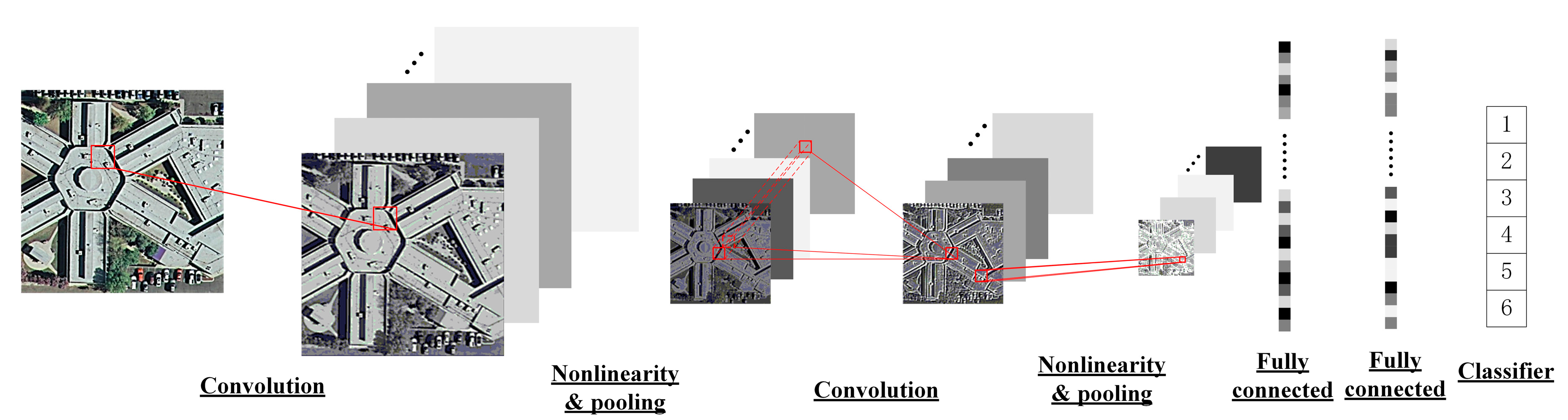
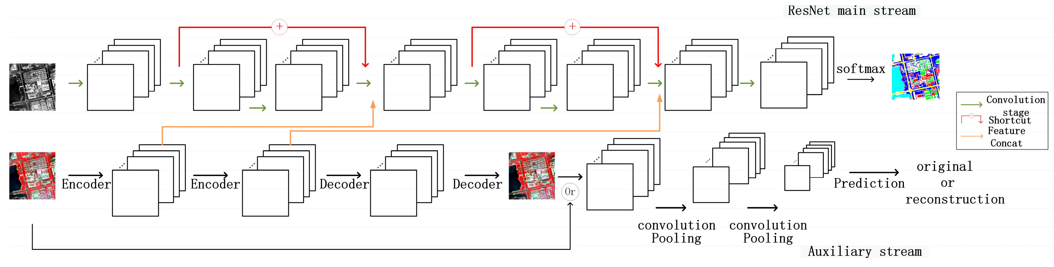
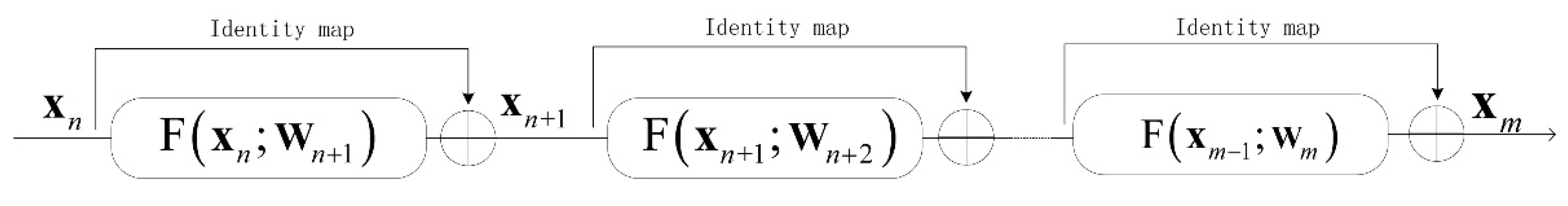
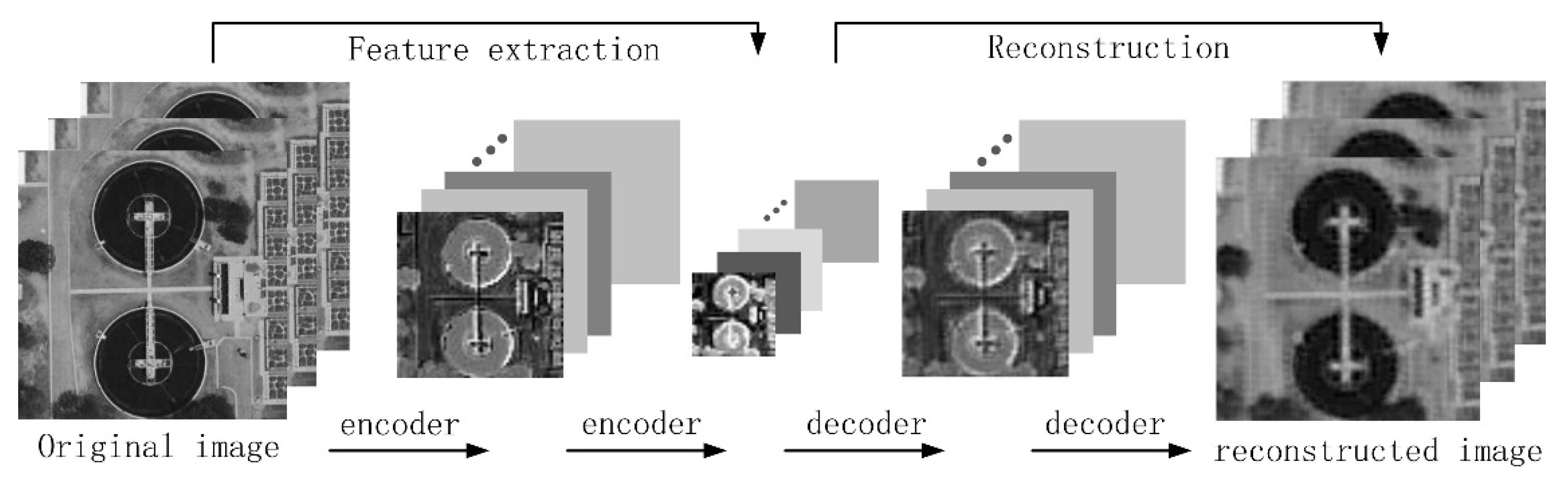
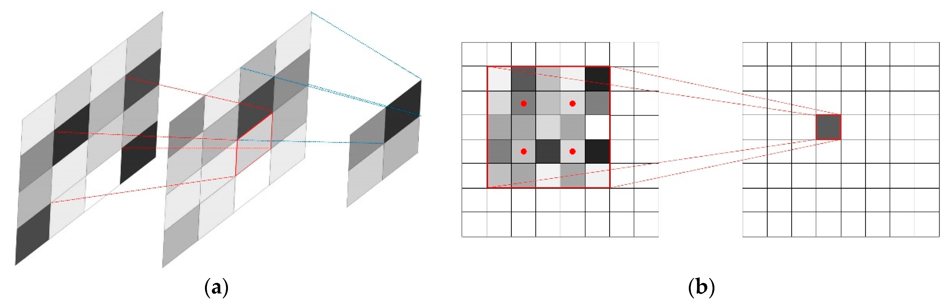
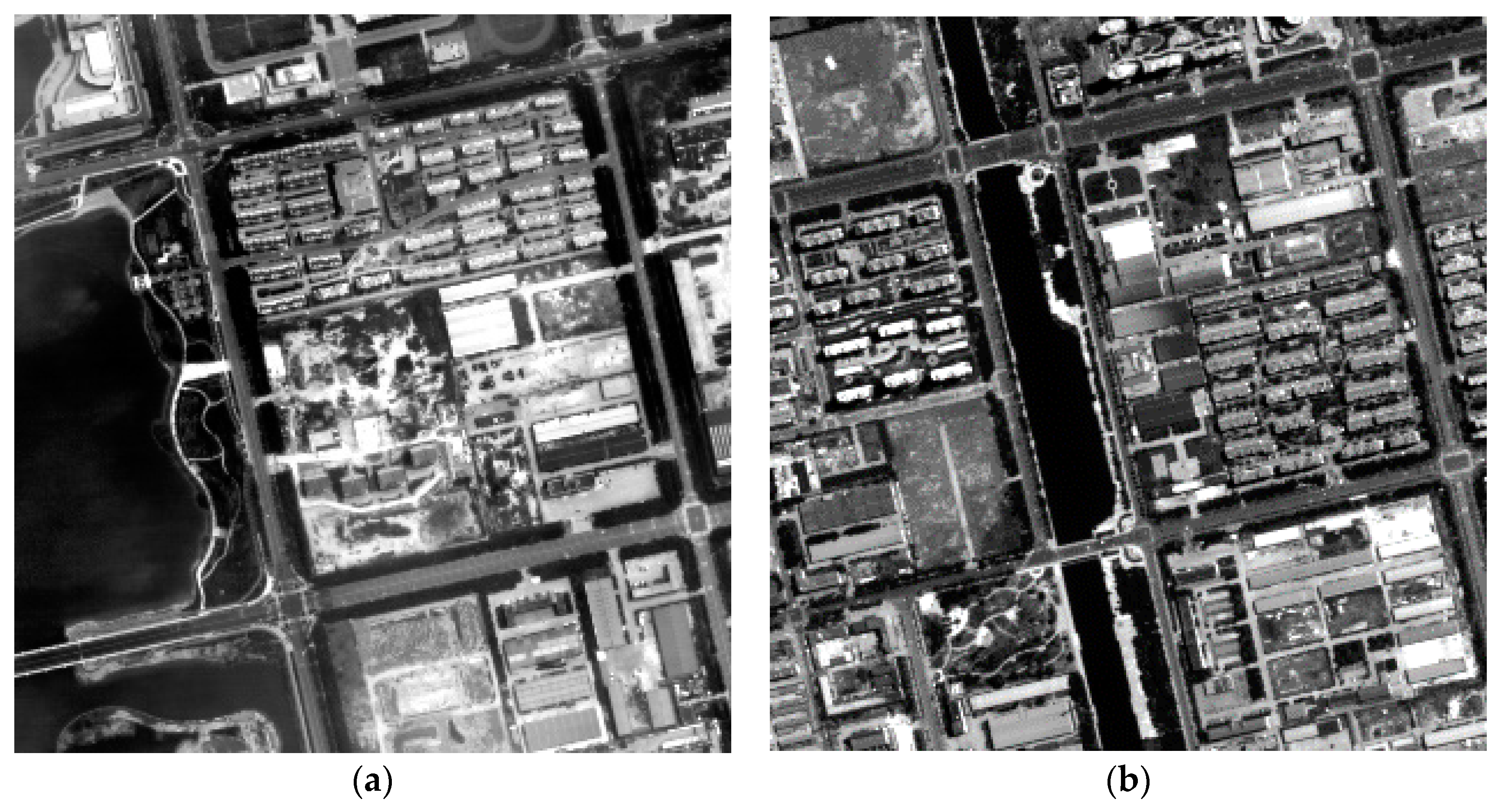
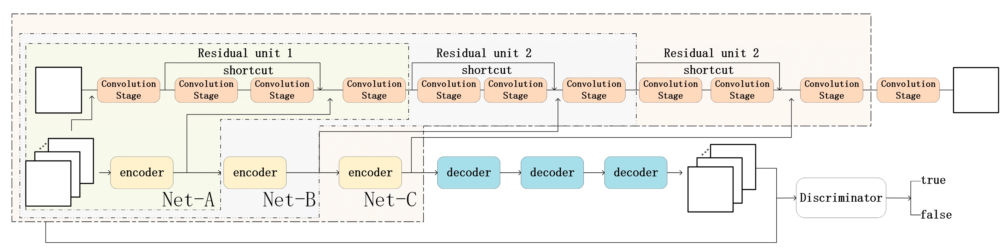
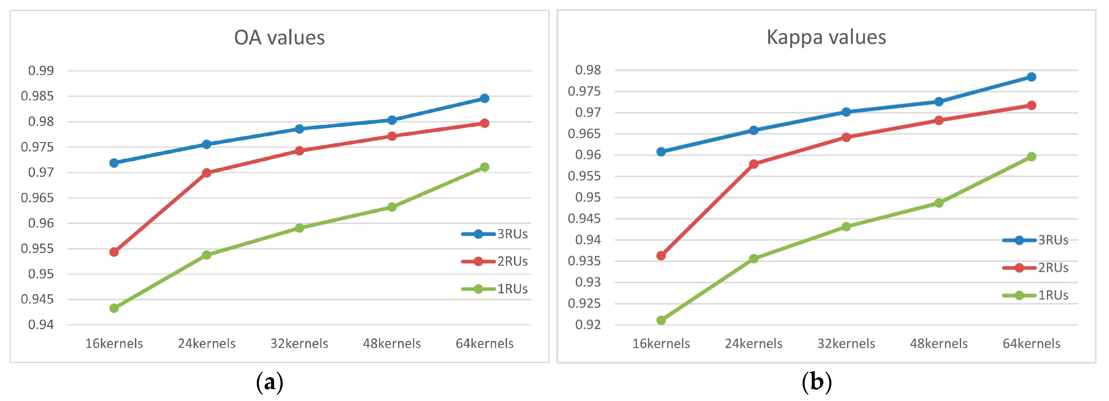
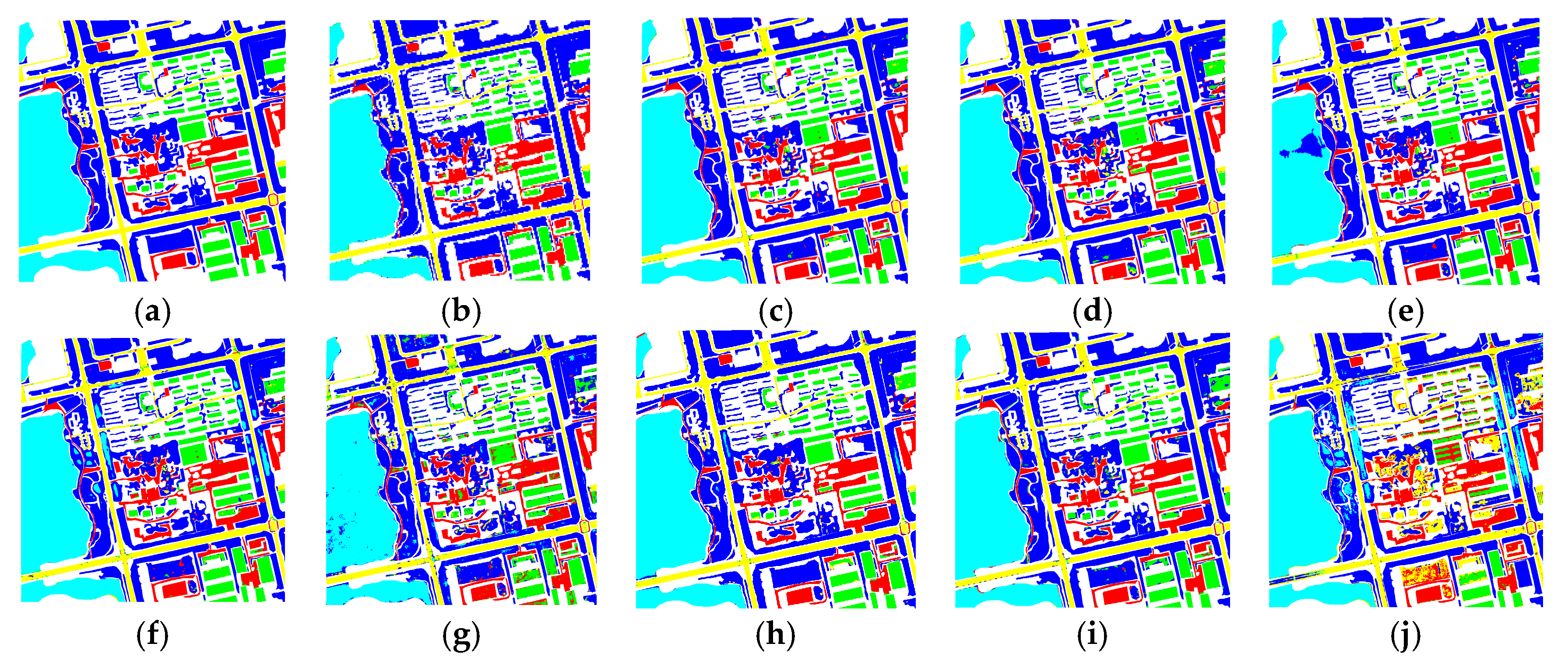
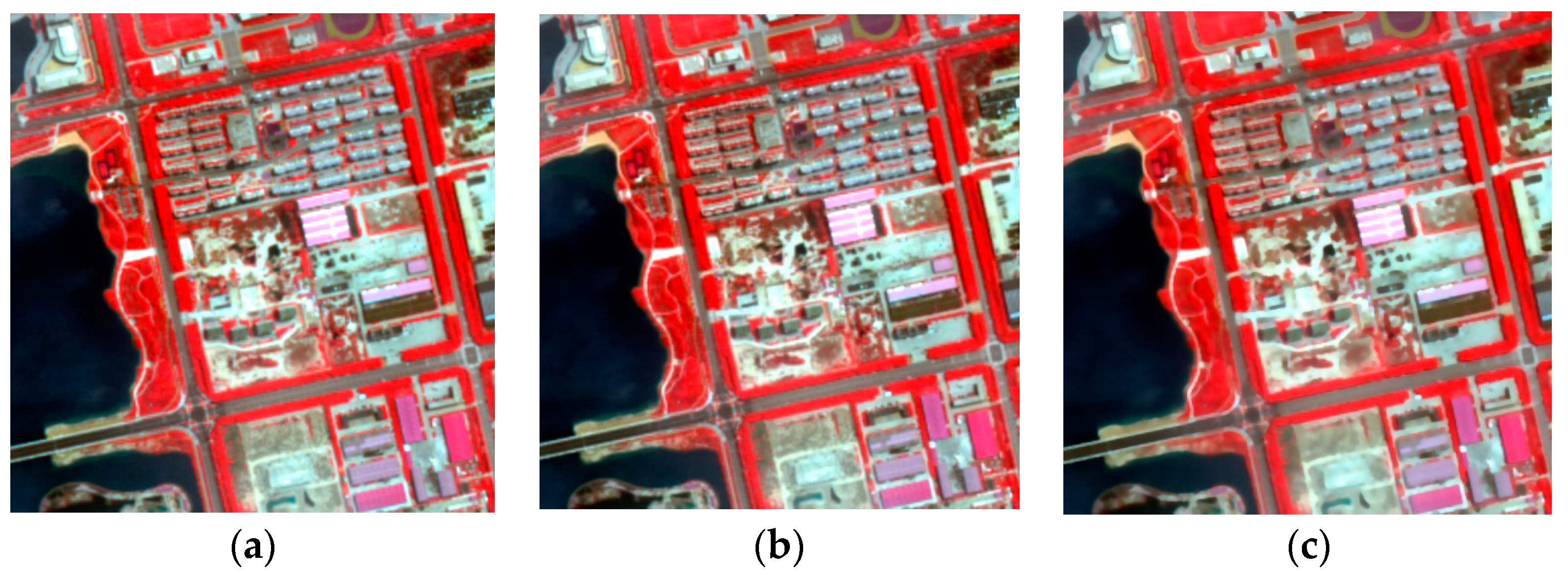
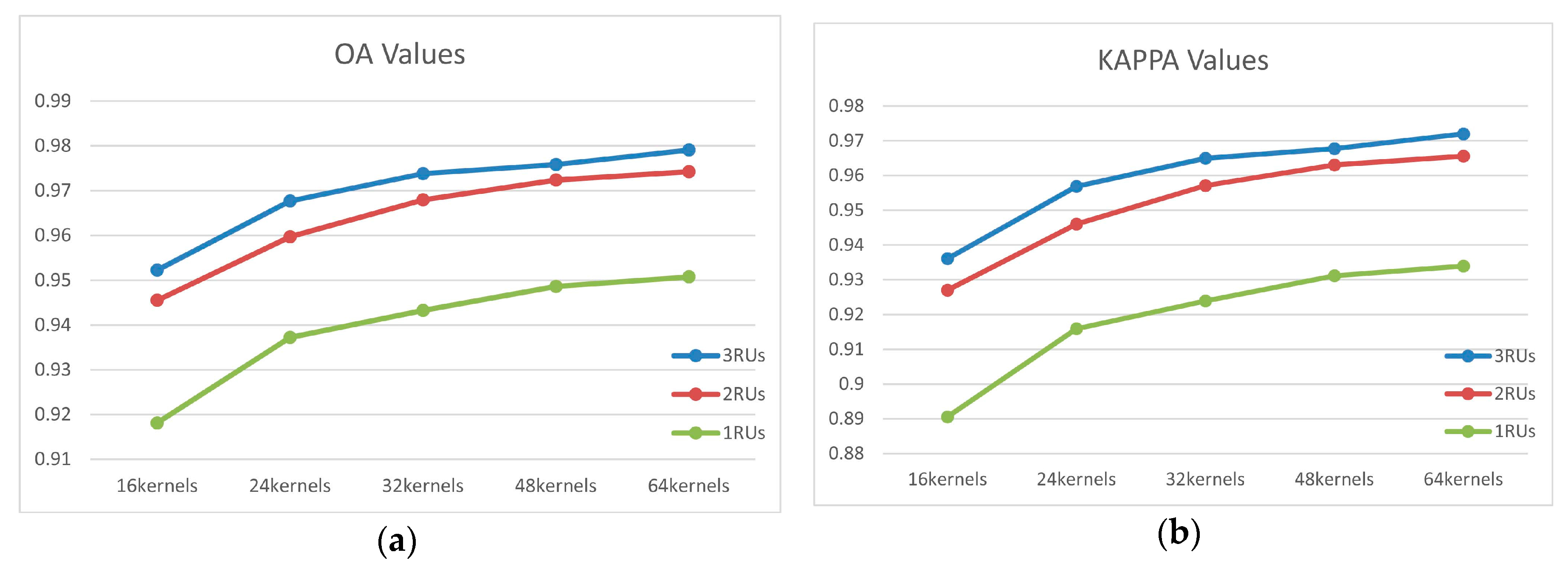
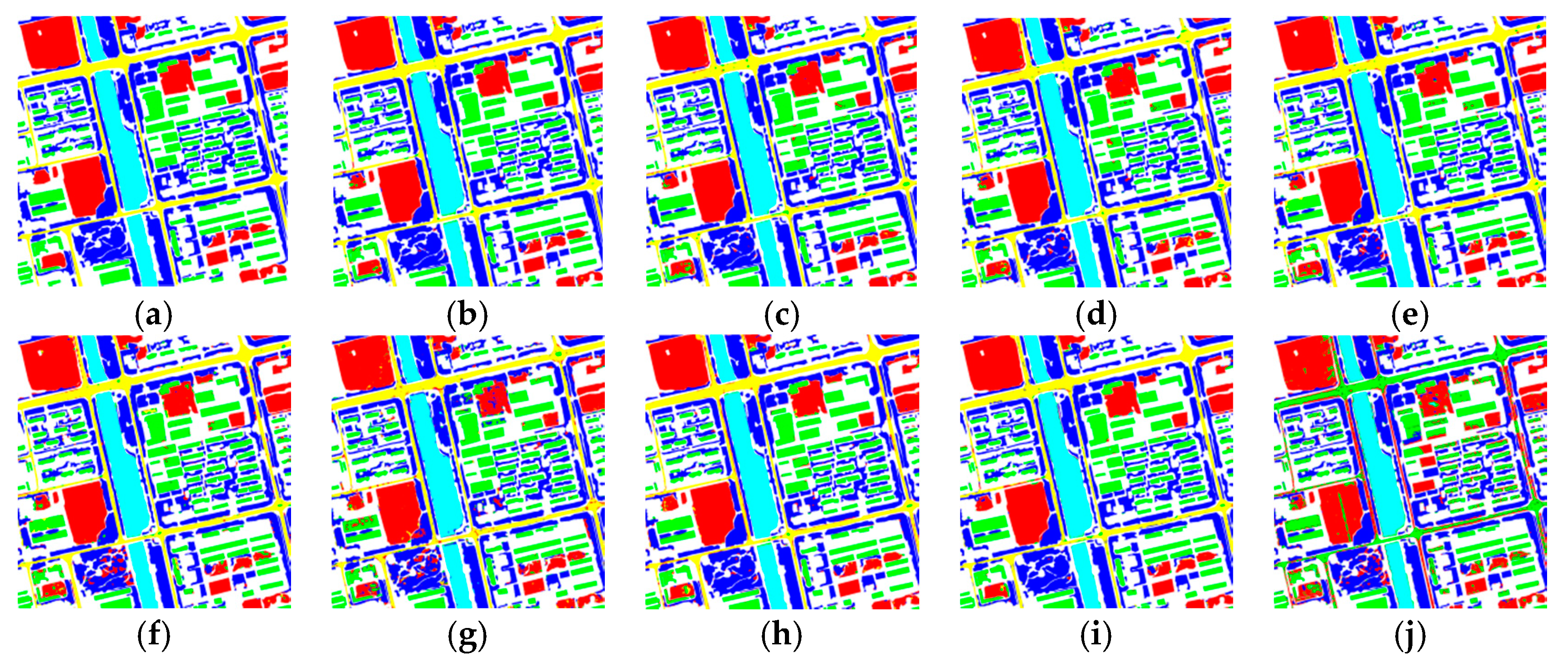
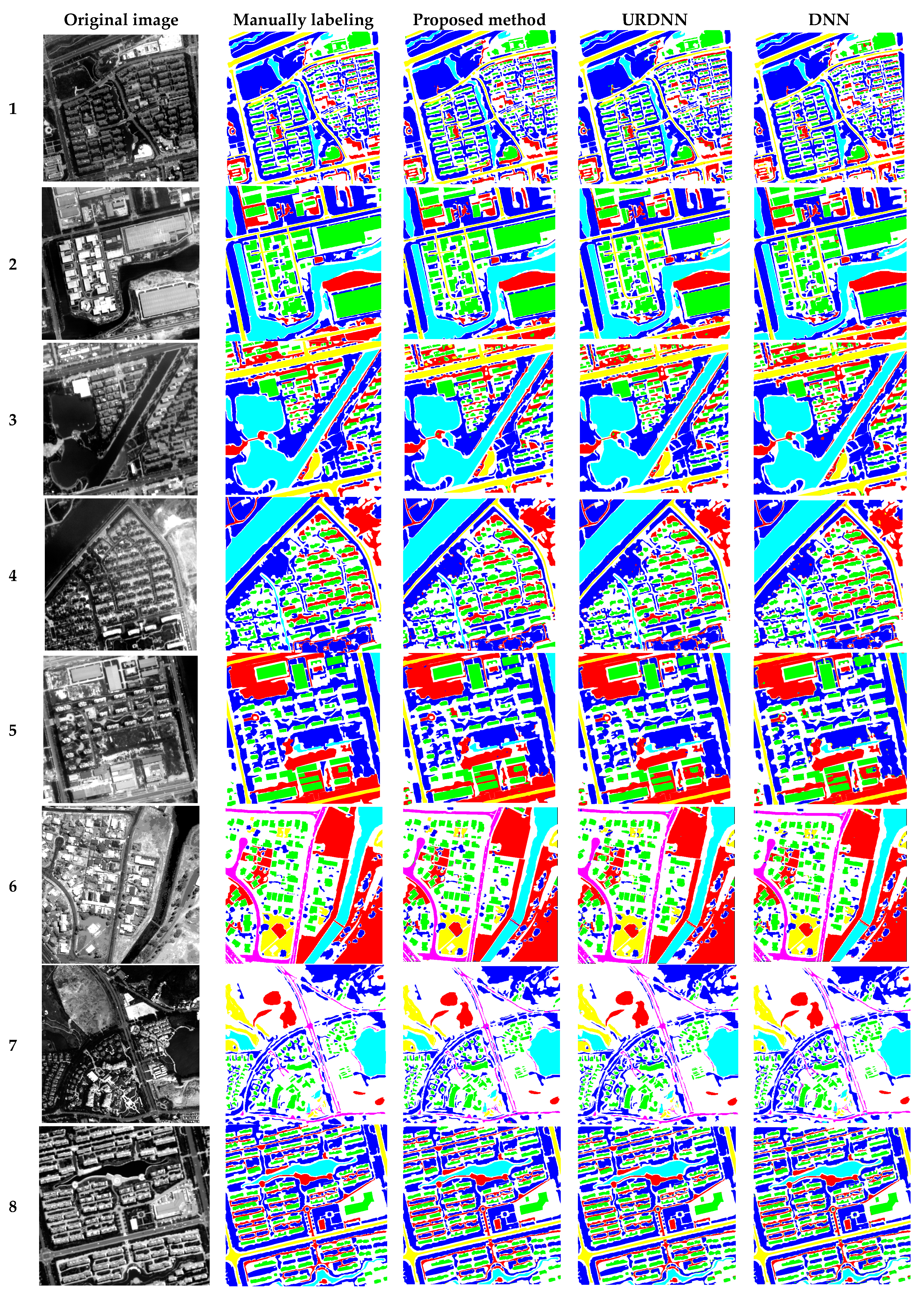
Table 1.
Reference data information for GF02 and BJ02 images.
| GF | Size 950 × 950 | BJ | Size 950 × 950 | ||||
|---|---|---|---|---|---|---|---|
| No. | Category | Mark Color | Number of Pixels | No. | Category | Mark Color | Number of Pixels |
| 1 | Water | Light Blue | 167,733 | 1 | Water | Light Blue | 87,937 |
| 2 | Tree | Blue | 290,717 | 2 | Tree | Blue | 252,783 |
| 4 | Bare Land | Red | 98,490 | 4 | Bare Land | Red | 137,217 |
| 5 | Building | Green | 94,208 | 5 | Building | Green | 135,225 |
| 6 | Road | Purple | 97,233 | 6 | Road | Purple | 104,802 |
Table 2.
OA values for GF02 experiments.
| Structure | 3 RUs | 2 RUs | 1 RUs |
|---|---|---|---|
| 16 kernels | 0.971894 | 0.954328 | 0.94325 |
| 24 kernels | 0.975533 | 0.96994 | 0.95376 |
| 32 kernels | 0.978585 | 0.974277 | 0.959088 |
| 48 kernels | 0.980324 | 0.97717 | 0.96319 |
| 64 kernels | 0.98456 | 0.97969 | 0.97106 |
Table 3.
Kappa values for GF02 experiments.
| Structure | 3 RUs | 2 RUs | 1 RUs |
|---|---|---|---|
| 16 kernels | 0.960788 | 0.936320 | 0.921105 |
| 24 kernels | 0.965855 | 0.957890 | 0.935615 |
| 32 kernels | 0.970160 | 0.964183 | 0.943148 |
| 48 kernels | 0.972604 | 0.968207 | 0.948716 |
| 64 kernels | 0.978463 | 0.971720 | 0.959660 |
Table 4.
Classification results for all comparative experiments.
| Method | OA | Kappa | Water | Tree | Bare Land | Building | Road |
|---|---|---|---|---|---|---|---|
| proposed method | 0.985 | 0.978 | 0.992/1.000 | 0.992/0.988 | 0.956/0.967 | 0.966/0.966 | 0.988/0.977 |
| without GAN | 0.975 | 0.966 | 0.995/0.999 | 0.972/0.988 | 0.967/0.928 | 0.953/0.949 | 0.978/0.953 |
| fusion | 0.969 | 0.957 | 0.985/0.998 | 0.963/0.985 | 0.976/0.909 | 0.947/0.942 | 0.972/0.943 |
| fusion without ResNet | 0.960 | 0.945 | 0.966/0.987 | 0.956/0.973 | 0.975/0.907 | 0.938/0.942 | 0.969/0.934 |
| multispectral | 0.959 | 0.943 | 0.991/0.961 | 0.945/0.986 | 0.967/0.901 | 0.929/0.947 | 0.967/0.929 |
| panchromatic | 0.924 | 0.894 | 0.955/0.970 | 0.933/0.945 | 0.894/0.885 | 0.844/0.818 | 0.927/0.889 |
| URDNN | 0.964 | 0.950 | 0.988/0.992 | 0.954/0.982 | 0.971/0.913 | 0.937/0.904 | 0.973/0.955 |
| deconvolution | 0.971 | 0.959 | 0.987/0.989 | 0.966/0.986 | 0.962/0.946 | 0.954/0.938 | 0.983/0.935 |
| SCAE + SVM | 0.811 | 0.743 | 0.981/0.856 | 0.781/0.923 | 0.901/0.721 | 0.402/0.887 | 0.864/0.556 |
Table 5.
Classification results for all comparative experiments.
| Method | OA | Kappa | Water | Tree | Bare Land | Building | Road |
|---|---|---|---|---|---|---|---|
| proposed method | 0.979 | 0.972 | 0.984/0.998 | 0.982/0.989 | 0.973/0.966 | 0.987/0.965 | 0.962/0.976 |
| without GAN | 0.974 | 0.965 | 0.995/0.998 | 0.974/0.990 | 0.959/0.956 | 0.980/0.954 | 0.967/0.960 |
| fusion | 0.969 | 0.959 | 0.994/0.998 | 0.973/0.989 | 0.959/0.943 | 0.976/0.944 | 0.940/0.962 |
| fusion without ResNet | 0.967 | 0.955 | 0.994/0.998 | 0.967/0.990 | 0.963/0.934 | 0.965/0.941 | 0.950/0.961 |
| multispectral | 0.956 | 0.942 | 0.997/0.998 | 0.939/0.991 | 0.960/0.899 | 0.963/0.937 | 0.960/0.943 |
| panchromatic | 0.939 | 0.918 | 0.986/0.993 | 0.916/0.972 | 0.943/0.861 | 0.969/0.937 | 0.922/0.933 |
| URDNN | 0.973 | 0.964 | 0.984/0.996 | 0.976/0.985 | 0.969/0.965 | 0.986/0.965 | 0.940/0.942 |
| deconvolution | 0.967 | 0.956 | 0.994/0.992 | 0.965/0.992 | 0.958/0.908 | 0.983/0.972 | 0.939/0.958 |
| SCAE + SVM | 0.787 | 0.713 | 0.957/0.982 | 0.920/0.970 | 0.890/0.647 | 0.806/0.585 | 0.000/0.000 |
Table 6.
Classification accuracy for all comparative experiments of 8 examples.
| No. | Method | OA | Kappa | Water | Tree | Bare Land | Building | Road | Grass |
|---|---|---|---|---|---|---|---|---|---|
| 1 | OUR’S | 0.976 | 0.959 | 0.998/0.921 | 0.983/0.999 | 0.951/0.897 | 0.955/0.968 | 0.978/0.959 | / |
| URDNN | 0.971 | 0.951 | 0.994/0.895 | 0.978/0.999 | 0.938/0.927 | 0.954/0.928 | 0.978/0.951 | / | |
| DNN | 0.965 | 0.942 | 0.994/0.936 | 0.988/0.999 | 0.923/0.856 | 0.897/0.965 | 0.967/0.901 | / | |
| 2 | OUR’S | 0.982 | 0.975 | 0.998/0.997 | 0.987/0.993 | 0.940/0.930 | 0.983/0.983 | 0.963/0.951 | / |
| URDNN | 0.964 | 0.953 | 0.988/0.995 | 0.961/0.994 | 0.942/0.908 | 0.960/0.984 | 0.979/0.787 | / | |
| DNN | 0.978 | 0.970 | 0.995/0.985 | 0.977/0.993 | 0.977/0.917 | 0.965/0.996 | 0.993/0.919 | / | |
| 3 | OUR’S | 0.981 | 0.975 | 1.000/1.000 | 0.987/0.999 | 0.942/0.960 | 0.959/0.929 | 0.985/0.951 | / |
| URDNN | 0.972 | 0.963 | 0.997/1.000 | 0.975/0.998 | 0.914/0.954 | 0.953/0.851 | 0.989/0.962 | / | |
| DNN | 0.969 | 0.958 | 0.995/1.000 | 0.969/0.998 | 0.945/0.892 | 0.939/0.890 | 0.956/0.975 | / | |
| 4 | OUR’S | 0.982 | 0.974 | 1.000/0.999 | 0.974/0.995 | 0.977/0.919 | 0.990/0.990 | 0.992/0.964 | / |
| URDNN | 0.975 | 0.964 | 1.000/0.999 | 0.963/0.995 | 0.969/0.899 | 0.987/0.988 | 0.986/0.790 | / | |
| DNN | 0.965 | 0.949 | 0.999/0.996 | 0.954/0.991 | 0.935/0.896 | 0.986/0.975 | 0.986/0.638 | / | |
| 5 | OUR’S | 0.973 | 0.960 | 1.000/0.954 | 0.973/0.995 | 0.977/0.956 | 0.963/0.953 | 0.990/0.971 | / |
| URDNN | 0.969 | 0.954 | 0.983/ 0.983 | 0.959/0.995 | 0.984/0.959 | 0.966/0.935 | 0.981/0.937 | / | |
| DNN | 0.950 | 0.926 | 0.980/0.980 | 0.930/0.995 | 0.973/0.945 | 0.947/0.898 | 0.991/0.831 | / | |
| 6 | OUR’S | 0.979 | 0.972 | 0.996/0.999 | 0.927/0.908 | 0.980/0.989 | 0.984/0.972 | 0.988/0.976 | 0.967/0.982 |
| URDNN | 0.977 | 0.966 | 0.997/0.995 | 0.932/0.859 | 0.978/0.992 | 0.977/0.969 | 0.982/0.969 | 0.954/0.959 | |
| DNN | 0.976 | 0.967 | 0.997/0.986 | 0.911/0.940 | 0.978/0.989 | 0.978/0.967 | 0.986/0.993 | 0.969/0.917 | |
| 7 | OUR’S | 0.989 | 0.985 | 0.996/0.997 | 0.990/0.992 | 0.998/0.998 | 0.995/0.984 | 0.935/0.951 | 0.996/0.989 |
| URDNN | 0.990 | 0.985 | 0.993/0.985 | 0.992/0.994 | 0.990/0.999 | 0.993/0.990 | 0.969/0.965 | 0.981/0.988 | |
| DNN | 0.987 | 0.981 | 0.993/0.972 | 0.985/0.995 | 0.990/1.000 | 0.994/0.983 | 0.979/0.943 | 0.974/0.997 | |
| 8 | OUR’S | 0.981 | 0.969 | 1.000/0.974 | 0.971/1.000 | 0.994/0.961 | 0.992/0.980 | 1.000/0.933 | / |
| URDNN | 0.973 | 0.956 | 0.999/0.986 | 0.962/0.999 | 0.986/0.961 | 0.986/0.919 | 1.000/0.945 | / | |
| DNN | 0.960 | 0.936 | 0.999/0.996 | 0.943/0.997 | 0.974/0.926 | 0.979/0.886 | 0.999/0.854 | / |
© 2017 by the authors. Licensee MDPI, Basel, Switzerland. This article is an open access article distributed under the terms and conditions of the Creative Commons Attribution (CC BY) license (http://creativecommons.org/licenses/by/4.0/).
Share and Cite
MDPI and ACS Style
Tao, Y.; Xu, M.; Zhong, Y.; Cheng, Y. GAN-Assisted Two-Stream Neural Network for High-Resolution Remote Sensing Image Classification. Remote Sens. 2017, 9, 1328. https://0-doi-org.brum.beds.ac.uk/10.3390/rs9121328
AMA Style
Tao Y, Xu M, Zhong Y, Cheng Y. GAN-Assisted Two-Stream Neural Network for High-Resolution Remote Sensing Image Classification. Remote Sensing. 2017; 9(12):1328. https://0-doi-org.brum.beds.ac.uk/10.3390/rs9121328
Chicago/Turabian StyleTao, Yiting, Miaozhong Xu, Yanfei Zhong, and Yufeng Cheng. 2017. "GAN-Assisted Two-Stream Neural Network for High-Resolution Remote Sensing Image Classification" Remote Sensing 9, no. 12: 1328. https://0-doi-org.brum.beds.ac.uk/10.3390/rs9121328
Note that from the first issue of 2016, this journal uses article numbers instead of page numbers. See further details here.