1. Introduction
In the past two decades, efforts have been made to decrease forest inventory costs by using data obtained from remote sensing technology. Airborne LiDAR (Light Detection And Ranging) is an active remote sensing technology that provides distance measurements between an aircraft (or any other platform) and the surface illuminated by the laser beam [
1,
2]. Due to its ability to generate 3D (three-dimensional) data with high spatial resolution and accuracy, the airborne small-footprint LiDAR is becoming a promising technique for modeling the forest canopies and thus for completing several inventory tasks [
3,
4]. Numerous methods or algorithms have been proposed to identify or detect individual trees or tree crowns using airborne LiDAR data. Raster-based approaches utilizing the canopy height model (CHM) derived from raw LiDAR data are widely adopted for individual tree segmentation [
5]. In a typical CHM-based scenario, a local maximum filter is used to detect treetops and then the individual tree crowns are delineated with a marker-controlled watershed segmentation scheme or a pouring algorithm [
6,
7,
8,
9,
10]. Region growing, as a category of simple region-based segmentation methods, can be adopted for segmentation of 3D point cloud generated by the LiDAR [
11] and it is the most common approach to segmenting trees in original LiDAR data [
1,
3,
12]. Extracting individual trees directly from the original LiDAR data can also resort to clustering-based methods. One of the most popular clustering methods is the
k-means algorithm, which aims to partition
n observations into
k clusters where each observation belongs to the cluster with the nearest mean by trying to minimize the overall sum of Euclidean distances of the points in feature space to their cluster centroids [
13,
14,
15]. Most of these methods fall into one of the two categories: raster-based approaches or point-based approaches. Usually, raster-based approaches are more automatic and require fewer parameters than point-based approaches and thus have a leading edge in processing speed, but they tend to merge crowns in dense stands of deciduous trees or fail to detect understory trees in a multi-layered forest as the process of producing a CHM could lead to loss of information from different levels in the canopy [
9]. Alternatively, point-based approaches work directly on the original airborne laser scanning (ALS) data (namely the “point cloud”, a discrete set of point locations) rather than rasterized images. This category of methods is preferable because it provides a promising way of producing relatively high accuracy by detecting smaller trees in the understory than CHM-based methods.
In recent years, mean shift-based clustering techniques have been applied in individual tree delineation using LiDAR data [
16,
17,
18,
19]. Mean shift is a powerful and versatile feature-space analysis technique and has found much interest in the image processing and computer vision community [
20,
21]. As it does not depend on any geometric model assumptions, its applications can be extended to the processing of unstructured point cloud data [
22,
23]. For example, Melzer explored the mean shift’s uses in LiDAR data processing and firstly utilized the mean shift procedure as a tool to automatically extract and reconstruct power lines from ALS point clouds [
22]. Different from the region growing method and the
k-means algorithm, mean shift does not require seed points and thus it is not sensitive to initializations. Moreover, the mean shift algorithm does not assume anything about the number of clusters and does not assume any predefined shape on data clusters, and the only parameter that has to be specified is the so-called kernel bandwidth for each attribute used. Therefore, it can handle arbitrarily shaped clusters. It is confirmed that the mean shift clusters can better indicate smaller or suppressed trees in the understory, which is not possible to do using other kinds of methods [
19]. For simultaneous segmentation of vertical and horizontal structures of forest canopies, Ferraz et al. proposed a multi-scale mean shift method where modes are computed with a stratum-dependent kernel bandwidth whose values are increased as a function of the vegetation layer’s height [
16,
17]. In a multi-layered Mediterranean forest mainly covered with eucalyptus and maritime pine trees, they announced an overall detection rate of 69.3%. The specific detection rates were observed to decrease with the dominance position: from 98.6% for the dominant trees to only 12.8% for the suppressed trees [
17]. A mean shift-based two-staged recursive computing scheme on the data sets in a defined complex multimodal feature space was employed to cluster points with similar vegetation modes together and an overall detection accuracy of more than 80% was reported in [
18]. Mean shift clustering was also utilized to construct small parts of trees in a two-tiered 3D segmentation of forest point clouds into segments associated with regeneration trees and up to 70% of the regeneration coverage in a multilayered temperate forest could be correctly estimated [
19].
For the mean shift clustering, calibration of the kernel bandwidth is very critical, since this parameter has a strong impact on the quality and speed of the decomposition and clustering. The mean shift procedure with a small kernel bandwidth is time-consuming but will lead to more distinct modes (small basins of attraction, more and smaller objects), while a large bandwidth has a fast convergent rate but will aggregate small structures into larger ones (small number of modes with large basins of attraction) [
16]. The calibration of an optimal value for the kernel bandwidth is actually a major challenge for the clustering techniques based on mean shift. Obviously, an adaptive selection scheme for the kernel bandwidth considering local structure information outperforms that using a single bandwidth for the whole feature space. Methods proposed in [
16,
17,
18,
19] are all fixed bandwidth mean shift procedures, where a single kernel bandwidth in a forest stand or a specific vegetation stratum is not adapted to heterogeneous crown sizes and thus could result in obvious under-segmentations or over-segmentations. Ferraz et al. designed a technique called 3D adaptive mean shift (AMS3D), in which three bandwidths of different sizes were applied to three forest layers: overstory, understory and ground vegetation, to decompose the entire point cloud into 3D clusters that correspond to individual tree crowns [
17]. Yet, such an approach is essentially based on fixed bandwidth mean shift procedures and not suitable for complex forest environments because the boundaries of the vegetation layers are fuzzy and difficult to identify. A self-adaptive approach calibrating the kernel bandwidth as a function of a local tree allometric model that can adapt to the local forest structure was developed also by Ferraz et al. in [
24]. It consists of two steps: in the first step, a limited number of easily recognizable individual trees are extracted from the LiDAR data to derive local tree allometry relating tree height to crown size and the second step uses the derived tree allometry model to provide the a priori information required by the AMS3D algorithm. However, detection of isolated individual tree samples would rely on a CHM-based and object-oriented approach, which requires complicated image analysis and processing. Furthermore, local allometric models established by linear regressions using estimated crown size data of individual tree samples might not be suitable for other types of forest.
In this paper, we propose an adaptive mean shift-based clustering scheme dedicated to the segmentation of 3D forest point clouds and identification of individual tree crowns. Our major contribution is in the development of a novel method to calibrate the adaptive mean shift procedure’s kernel bandwidth by applying a “divide and conquer” processing strategy directly on the raw point cloud to improve computational efficiency. The kernel bandwidth of the adaptive mean shift procedure can be changed according to estimated crown sizes of distinct trees without relying on any local allometric model. To acquire approximate information about local canopy structure, some processing is a must: each test area is firstly divided into small spatial units, called “partitions” here, by performing a single-scale mean shift-based coarse segmentation, where an original small square grouping technique is used to accomplish rough partitioning of the region of interest; and then rough estimation of crown sizes based on another original 2D (two-dimensional) incremental grid projection technique is performed in each partition, providing a basis for dynamical calibration of the kernel bandwidth. Our proposed method is experimentally applied to small-footprint LiDAR data acquired in a field survey performed in an evergreen broad-leaved forest located in South China, and we validate its performance using 10 sample plots.
3. Methodology
3.1. Mean Shift Theory
The mean shift is a recursive computing procedure using a non-parametric probability density estimator based on the Parzen window kernel function [
21]. When used for clustering, mean shift treats the feature space as an empirical probability density function and considers the input set of points as sampled from the underlying probability distribution. Accordingly, clusters are defined as areas of higher density than the remainder of the data set and dense regions in feature space correspond to the modes (or local maxima) of the probability density function. The aim of the mean shift procedure is to move each data point to the densest area in its vicinity by iteratively performing the shift operation based on kernel density estimation. Eventually, the points will converge to local maxima of density, or that is to say, mean shift will associate each point with the nearest peak of the surface reflecting the data set’s probability density distribution. Mean shift is essentially a hill climbing algorithm which involves shifting a kernel iteratively to a higher density region until convergence. The detailed mathematical derivation of the mean shift procedure is given in the
Appendix, or refer to [
17].
Mean shift works by placing a kernel on each point in the data set. The kernel, a function that determines the weight of nearby points for re-estimation of the mean, is iteratively shifted with a bandwidth (namely the diameter of the hyper-sphere) to a denser region until it converges to a stationary point. Choice of the kernel bandwidth—
h is very critical. Many adaptive or variable bandwidth selection techniques have been proposed for mean shift with regard to 2D imagery analysis. There is a variable bandwidth technique that imposes a local structure on the data to extract reliable scale information by maximizing the magnitude of the normalized mean shift vector [
26]. Separability in feature space or local homogeneity can be exploited to adaptively select bandwidth parameters for remote-sensing image classification and object recognition [
27]. The local scale and structure information of the neighborhood around individual samples can also be utilized to calibrate the kernel bandwidth in an adaptive mean shift procedure to find arbitrary density, size and shape clusters in remote sensing imagery [
28].
3.2. Methodology Workflow
In this paper, we develop an adaptive mean shift scheme to segment the forest point clouds into 3D clusters and properly identify and extract individual tree crowns over a multi-layered forest in China. The mean shift procedure builds upon the concept of kernel density estimation, where the kernel is a weighting function to estimate the probability density function of a random variable. Extraction of individual trees from LiDAR data utilizing the mean shift procedures implies finding modes in a huge data set by performing analysis of a feature space, which is constituted by feature vectors extracted from the the original 3D point cloud data. Definition of the feature space is an issue in the mean-shift based clustering. As the tree in a forest is usually modelled as a porous medium and a linear structure, very much different from an object with piece-wise continuous surfaces [
29], surface features—such as texture, local curvature and normal vector—will fail to function and the only feature that can be exploited is each point’s spatial location, whose mutual distance denotes spatial coherence and connectivity. Similar to the work reported in [
17,
24], pure spatial 3D coordinates are adopted to constitute the feature space in this study.
Using a single or multi-scale kernel bandwidth over the entire space is not optimal for the analysis of forest environments, because one or several global values might result in under-segmentations (a cluster assigned to more than one field measured trees) or over-segmentations (a single tree segmented into several LiDAR clusters). An approach for adaptive calibration of kernel bandwidth should be developed to deal with complex forest environments. We realize that the kernel bandwidth in the spatial domain should reflect the size of each tree crown. However, it is difficult to acquire exact quantitative information about each individual tree prior to the clustering analysis. Since the bandwidth calibration is critical, in this paper, we focus on designing a novel method to calibrate the kernel bandwidth in an adaptive mean shift-based computational scheme of 3D forest point cloud segmentation, which does not rely on a rasterized digital model such as CHM or canopy maxima model (CMM), but works directly on the original point cloud data and requires no expensive computation. Considering the time complexity of the mean shift algorithm is using big O notation, where T is the number of iterations and N denotes the data set’s size, a “divide and conquer” strategy is adopted in this method to reduce the computational load by partitioning a large area into smaller ones and perform the standard mean shift procedure in the small area.
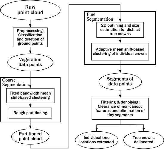
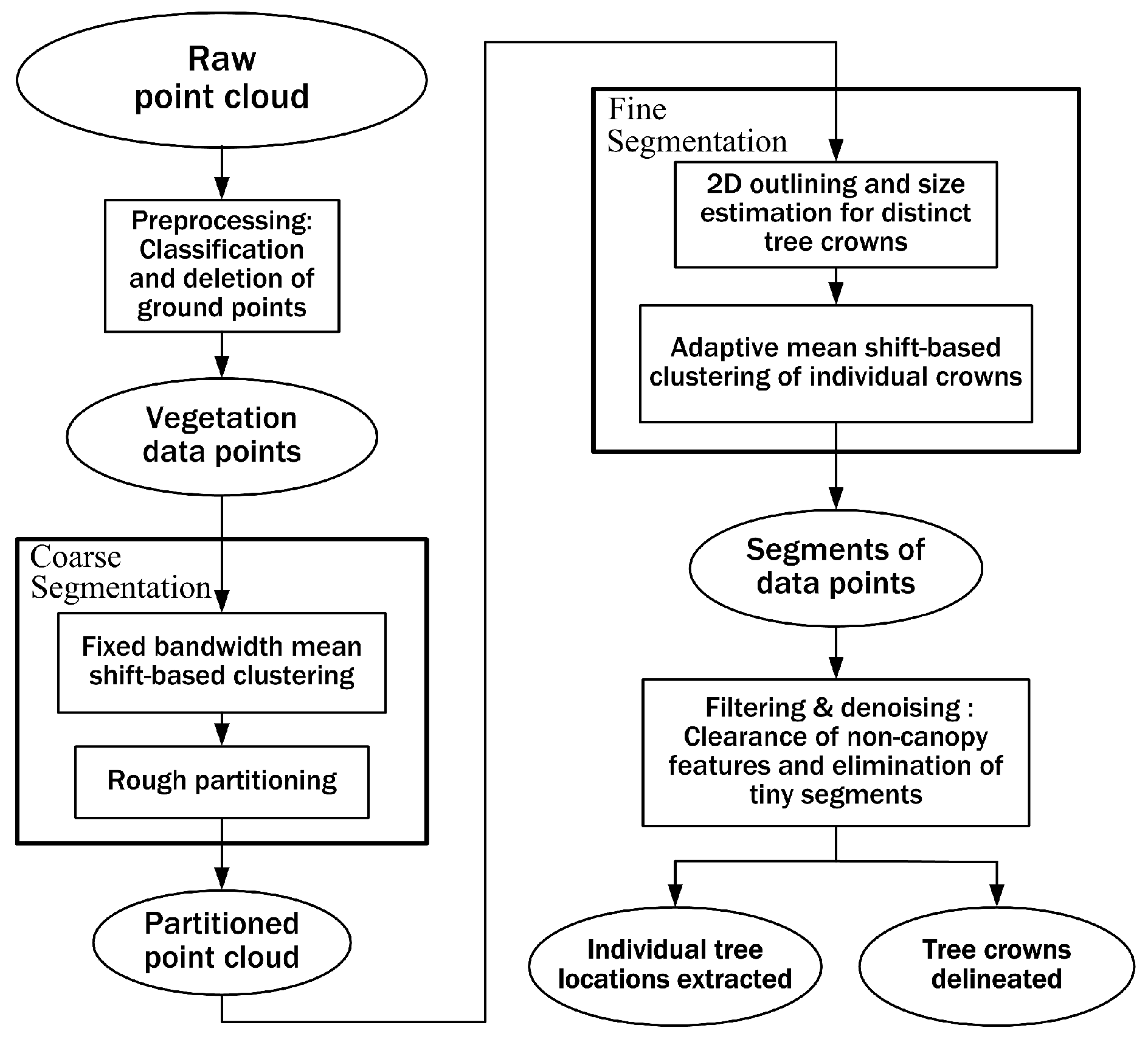
Taking into account all necessary mathematical processing used in this study, we present a flowchart of methods used in this study, as illustrated in
Figure 2, where the ellipses represent data or parameters and the rectangles represent processes or calculations. From the point of view of image segmentation, our proposed mathematical scheme is mainly a two-staged sequential segmentation procedure: coarse segmentation and fine segmentation. The single-scale mean shift-based area partitioning can be deemed a process of coarse segmentation while the adaptive mean shift-based clustering implements a fine segmentation process. The preprocessing step has been mentioned in
Section 2.2 and other processing steps will be described in detail in the following part of this section.
3.3. Rough Partitioning of Test Area
Due to the huge amount of point cloud data, it is computationally intensive to analyze all the points for the whole test area in one step. Therefore, the first stage of the two-staged sequential segmentation is to partition the 3D space over the forest area under test into many heterogenous vertical spatial units with irregular column-like shapes, each of which includes at least one actual tree. The sizes of the spatial units are much smaller than that of the original test area and thus when we perform a more thorough analysis on these small spatial units, which implies more complex mathematics, the total computational load could be reduced to a range that can be affordable. The aim of the rough partitioning is to obtain rough information about tree distributions by performing coarse segmentation and draw a sketch of the forest for each test subplot, where local structure information can be extracted to provide the basis for the subsequent variable bandwidth mean shift procedures. This processing stage consists of two steps: single-scale mean shift clustering and cluster-based spatial partition. The basic idea behind the methods is to divide a portion of the data set into several clusters, which can reflect the basic structure of one or several trees, with a small computational cost and then expand these clusters to the whole data set by exploring the spatial neighborhood relation between data points. Not the entire LiDAR data set is used in the two steps. The whole data set is divided into three parts according to the nature of returned signals: the first pulse data, the last pulse data and the intermediate pulse data. As the intermediate pulse data depict the internal spatial structures of tree crowns or lower vegetation, it can be used alone in the first step. The data contained in LiDAR return’s first echoes mainly reflect the information about the vegetation surface and they can be employed to estimate the maximum tree height and accomplish the rough partitioning in the second step.
In the first step, a fast mean shift procedure is utilized to achieve the goal of rough partition. In order to reduce computing expense and accelerate processing speed, only a part of the data set, the intermediate pulse data, is extracted to constitute the input set of points on which the mean shift segmentation is performed. For the same purpose of speeding up the process, the simplest kernel function—the uniform (or flat) kernel, which implies that all observations in the neighborhood of a data point are given the same weight—is used in this processing step. Thus, mean shift-based clustering analysis is performed in the three-dimensional Euclidean space using a uniform kernel function:
where,
x denotes the data point and
is a single-scale kernel bandwidth or window size. Owing to the lack of any information about forest structures in advance, a fixed kernel bandwidth setting is adopted in this stage. We determine the fixed value for the mean shift’s kernel bandwidth according to the maximum tree height for a particular subplot, which can be estimated by finding
highest points (considered as tree tops) in the LiDAR data set preserving just the first returns and then taking the average of these points’ elevation values. The value of
relies on the density of the raw point cloud. According to our experiments, a value of 30 is the ideal value for a data set with an average of 15 points per m
. Because a single tree in the woods, with smaller crown size than the one growing alone, usually assumes a high and straight form and its aspect ratio (i.e., the ratio between the crown diameter and height of the tree) is far less than 1, the kernel bandwidth should be set to a value less than the maximum tree height:
where,
is the estimate of the maximum height for trees in a specific subplot and
Q is a positive constant. To avoid over-segmentation that implies segmenting a single tree into several segments,
Q should be a number of less than 1 and its specific value will be discussed in
Section 4.2.
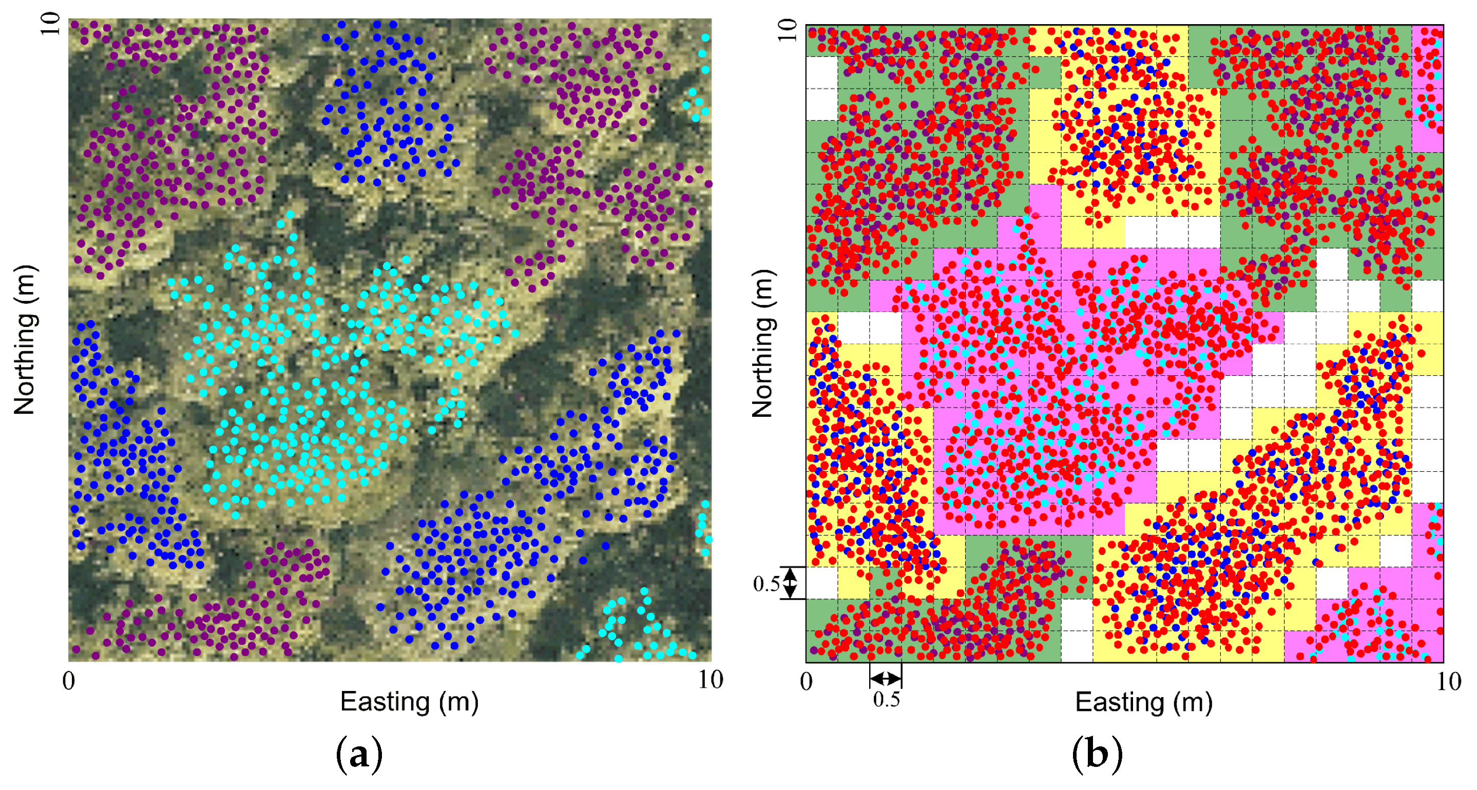
The single-scale mean shift procedure mentioned above would yield many segmented clusters of points extracted from the LiDAR’s intermediate pulse data.
Figure 3a shows an example of these mean shift clustering results for a small selected area (10 m × 10 m). As can be seen from this map, the specific middle pulse data set has been divided into several distinct clusters rendered in different colors. However, it is not enough to perform 3D space division of the forest area with only these clusters because the contour profile of an actual tree crown is larger than the shape from a cluster of the middle pulse data point. The first pulse data from the vegetation surface should be added to complete the rough partitioning in the subsequent step. This step is to divide the horizontal plane into small squares of identical sizes, assign each data point (either the intermediate pulse data or the first pulse data) to a specific square and finally group these squares into different partitions based on the mean shift clustering results. Such a technique, called the small square grouping technique in this paper, is illustrated in
Figure 3b. The data sets within the region of interest, formed by both the first and intermediate returns with points lower than 2 m excluded, are all projected onto the horizontal plane, which is divided into identical squares with sizes of 0.5 m × 0.5 m. Each individual square might contain one or several points from the first returns and/or the middle echoes. For a specific square, if there is no point in it, leave it alone. If the square contains at least a middle pulse data point, it will be associated with the cluster that the point belongs to. If there is only the first pulse data in the square, assign the nearest middle pulse point to it and then associate it with the corresponding cluster.
3.4. Estimation of Distinct Tree Crown Sizes
The above described rough partitioning process adopts a fixed bandwidth mean shift algorithm, whose global kernel bandwidth is far greater than the canopy size, and thus obvious under-segmentations would inevitably come into being. Such under-segmentations can be reduced by using a variable bandwidth mean shift algorithm in the subsequent processing stage, which automatically calibrates the kernel bandwidth to the local spatial structures of the forest canopy. Thus, a more sophisticated mean shift clustering scheme with an adaptive kernel bandwidth optimized for local canopy structure should be designed to deal with complex patterns in each coarsely segmented forest partition. The adaptive mean shift procedure necessitates information about the local canopy structure for each partition, which provides a basis for adaptive determination of the kernel bandwidth. There exists a method to derive tree sizes from linear fitting equations to locally calibrate the bandwidth model [
24]. However, since this method assumes that there is a linear relationship between tree height and both crown depth and crown width, which is not the case for many forest scenarios, it is essentially an estimation of tree allometry. Actually, it is impossible to accurately extract data of individual tree crown sizes for a particular forest area prior to complete clustering of individual trees.
In this section, we propose a novel method to roughly estimate the size data of distinct tree crowns adopted in the second segmentation stage, which works directly on the point cloud and does not resort to raster images and sophisticated image processing techniques. The goal of this processing step is to identify distinct tree crowns in a partition, delineate their approximate 2D profiles and determine numerical values as the estimates of these tree crown sizes. Considering that the tree crowns in the study area assume different shapes (e.g., cone, umbrella, spindle, irregular shape, etc.), for the sake of processing simplicity, we model these crowns as spheres or hemispheres. Thus, the estimation problem can be reduced to find the maximum approximate intercepting area for each distinct tree crown and determine its effective diameter. The first returns are selected from the data points, and as they are most likely to be from tree canopy surfaces, these first pulse data are utilized to perform such an estimation to minimize the computational cost. This process is divided into two steps: 2D outlining of distinct tree crowns and determination of the effective crown diameter.
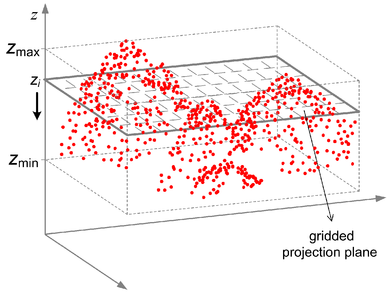
Firstly, rough boundaries of all distinct tree crowns in a partition are outlined by a simple region growing method based on incremental grid projection that we put forward particularly for this study. As shown in
Figure 4, suppose there is a plane (or screen) horizontally suspended over a partition of the forest area under study, project all the first pulse data points downward onto the plane and the 3D spatial distributions of the tree crowns will be reduced to 2D horizontal features on the plane. The projected 2D clusters on the horizontal plane represent the distribution of tree crowns at a certain height level and they will increase as the horizontal plane moves from top to bottom. The elevation value (
z coordinate) of the horizontal gridded plane decreases in a uniformly discrete mode, which implies shifting the projection plane at equal spacing from top to bottom. All of the points above the height-variable plane in the first return data set are projected downward onto this plane. It is possible to get the 2D horizontal distribution of individual tree crowns at different height levels when more than one 2D horizontal projections are available. Define
and
as the minimal and maximal coordinate values respectively in the
z-axis of the axis-aligned minimum bounding box for the data set, and
I as the total number of shift layers (each layer corresponds to an iteration of the region growing process), and then the elevation value for the projection plane used in the
i-th shift can be determined as
To speed up the whole estimation process, a small positive integer not exceeding 10—say, six or eight—should be adopted as the value of I in this study.
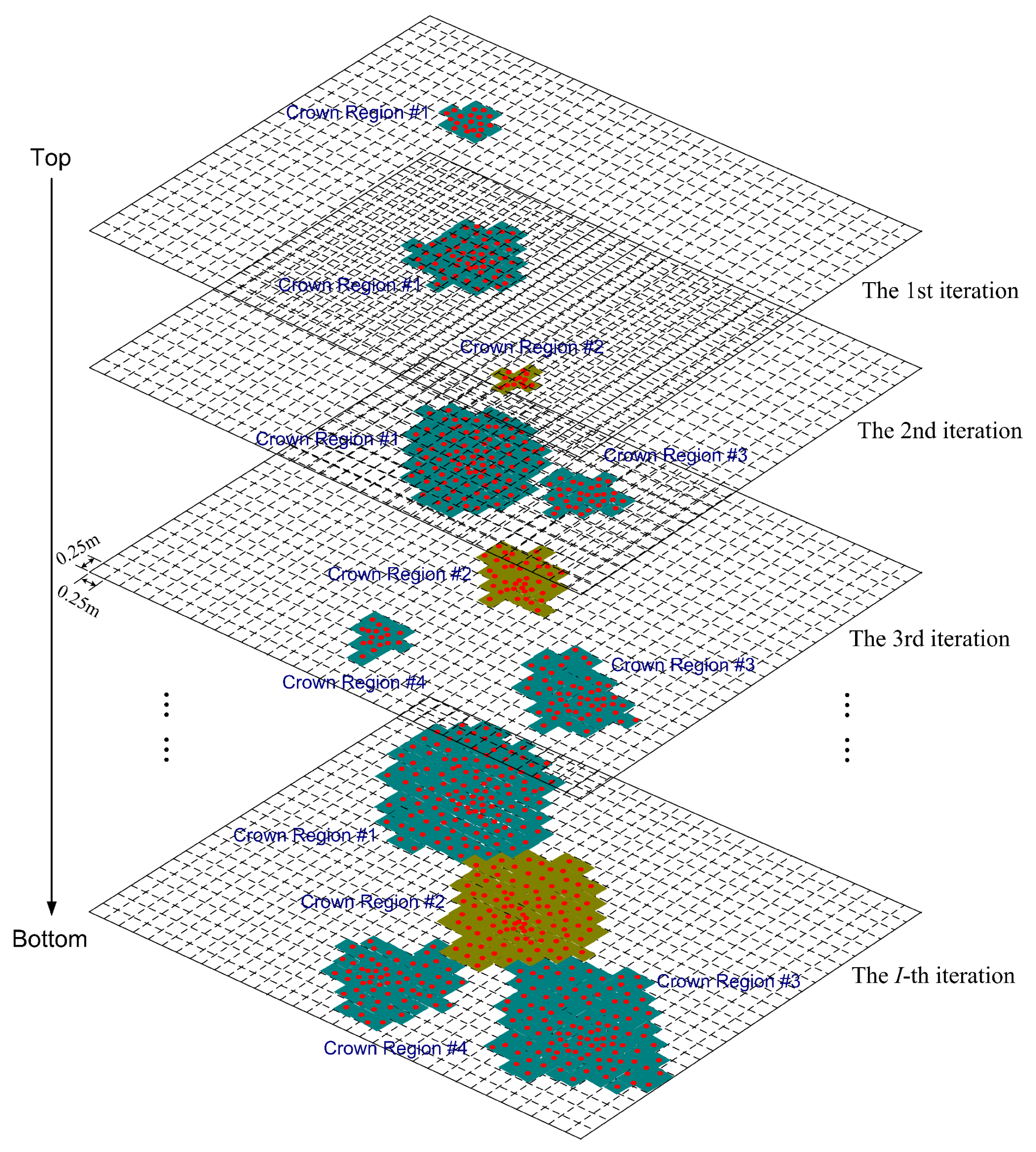
In order to simplify further analyses, the plane is divided into small grids by a raster net and points within the partition are mapped into grid cells, which can be regarded as pixels of an image. A non-empty cell (containing one or more projected points) is marked as a set pixel while an empty cell corresponds to an unset pixel. Thus, a series of 2D horizontal binary images can be generated. The clusters on the horizontal projection image at each layer represent the distribution of tree crowns in the correspondent height level. Therefore, a distinct tree crown should be visible at the same location of several vertical neighboring layers. The basic concept of the simple region growing method is to trace the presence of crown outlines on the binary images from top to bottom through projection images at different height levels. Outlines of the crown at the upper layers will present a cluster feature on the projection image, thus the task of detecting a distinct tree crown turns to an issue of extracting cluster feature of the treetop and tracing the crown outline from top to bottom.
Figure 5 depicts an example of such a region growing process, whose aim is to obtain an approximate intercepting area in terms of grid cell numbers for each distinct tree crown. The axis-aligned 2D horizontal plane is divided into grid cells with identical size of 0.25 m × 0.25 m. In each iteration, points no lower than the elevation of the moving projection plane are vertically mapped to their corresponding grid cells, and each non-empty cell might be determined as a new seed, if the distance from the existing clusters exceeds the threshold value of
, or else it would be added into an existing group based on spatial adjacency using a morphological analysis. The last iteration completes the region growing process and the area enclosed by the outmost grid cells in a region will be considered as the estimate of the intercepting area for a particular tree crown. Let
be the number of grid cells contained in a grown region, and the approximate intercepting area for the corresponding tree crown will be
, whose unit is m
. Thus, the effective crown diameter for a particular tree can be estimated as
where
r denotes the index number of a particular distinct crown region.
3.5. Adaptive Mean Shift-Based Clustering
With the estimated tree crown diameters, which reflect the local canopy structure in a forest area of interest, we can perform an adaptive mean shift analysis on an entire data set, using a combination of the first, intermediate and last pulse data points whose elevations are above 2 m, in the three-dimensional geometrical space for each partition. The aim of this adaptive mean shift procedure is to cluster points with similar modes (in the forestry scenario, the term “mode” has close relations with each single tree’s location and structure) together and delineate individual tree crowns. Euclidean distance between each point and a stationary point (represent some mode) is used as the measure of a tree’s spatial and structural properties. As mentioned previously, due to different crown shapes assumed by different tree species in the study area, we use a spherical kernel instead of a cylinder-shaped kernel proposed in [
17]. Such a unified spherical kernel, although at the expense of a little modeling performance, will facilitate mathematical processing. The uniform kernel is no longer used again because it is reasonable to attribute more weights to points that are near to that mean shift point and less weight to distant points at the stage of fine segmentation. As the Gaussian or normal function has excellent mathematical properties and similar characteristics with the points from a tree crown in statistical distributions and peak shapes, we choose the truncated, multivariate Gaussian function as the kernel (or window) function
where
is the variable kernel bandwidth that will adapt to the estimate of each crown diameter.
Let
be the input data set of the three-dimensional feature space. Run the mean shift computation on the data set
for each data point
and each iterative process will converge towards their corresponding stationary points or modes. Let
denote the data set of mean shift points, i.e., values at point
after its mean shift iteration. The detailed mean shift procedure proposed for the identification and delineation of individual trees is described as follows:
- I.
Specify a value for the allowable error—ε (set to 0.0025). Gaussian kernels are also associated with data points in the feature space.
- II.
For each point , execute the following computations:
- —
Initialization: associate a mean shift point with the point , and initialize it to coincide with that point. Let and , where t denotes the current number of mean shift iterations.
- —
For (c represents the word “convergence”), repeat the following three steps until convergence.
- —
Map the point
to the horizontal gridded projection plane defined in
Figure 4 and
Figure 5 to see which distinct crown region it belongs to. If this point is not in any region, associate it with the crown region nearest to it. Assume the corresponding crown region has the index number of
r, and then determine the variable kernel bandwidth as follows:
where
B is a constant coefficient of greater than 1 and less than 2.
- —
Calculate the mean shift vector:
- —
Update the mean shift point:
stopping when
is less than the specified value of
ε.
- —
Set .
- III.
Merge all modes whose mutual distance is less than the specific value of the variable kernel bandwidth, i.e., closer than , by concatenating the basins of attraction of the corresponding stationary points, to produce the clusters .
3.6. Removal of Non-Canopy Features
Application of the above described mean shift procedures in the forest point clouds would result in different types of vegetation segments of a sample area: tree canopy, shrubs, bramble, weeds and grasses, etc. Since our study focuses on the identification and delineation for trees, the non-canopy objects are the unwanted surface features whose data points should be recognized, marked and then cleared. Considering that the non-canopy features lie in the undersized vegetation strata, we could identify these objects by deciding whether their heights fall in a predefined height range whose upper limit is a preset threshold value—. The points belonging to these non-canopy features are not taken into account to final decisions. This step would remove the scrubby layers which are usually denser than the higher vegetation layers. Tiny segments containing less than a given number of data points, , should also be eliminated. These filtering operations would improve the ultimate detection results by eliminating possibly detrimental influences of non-canopy data points.
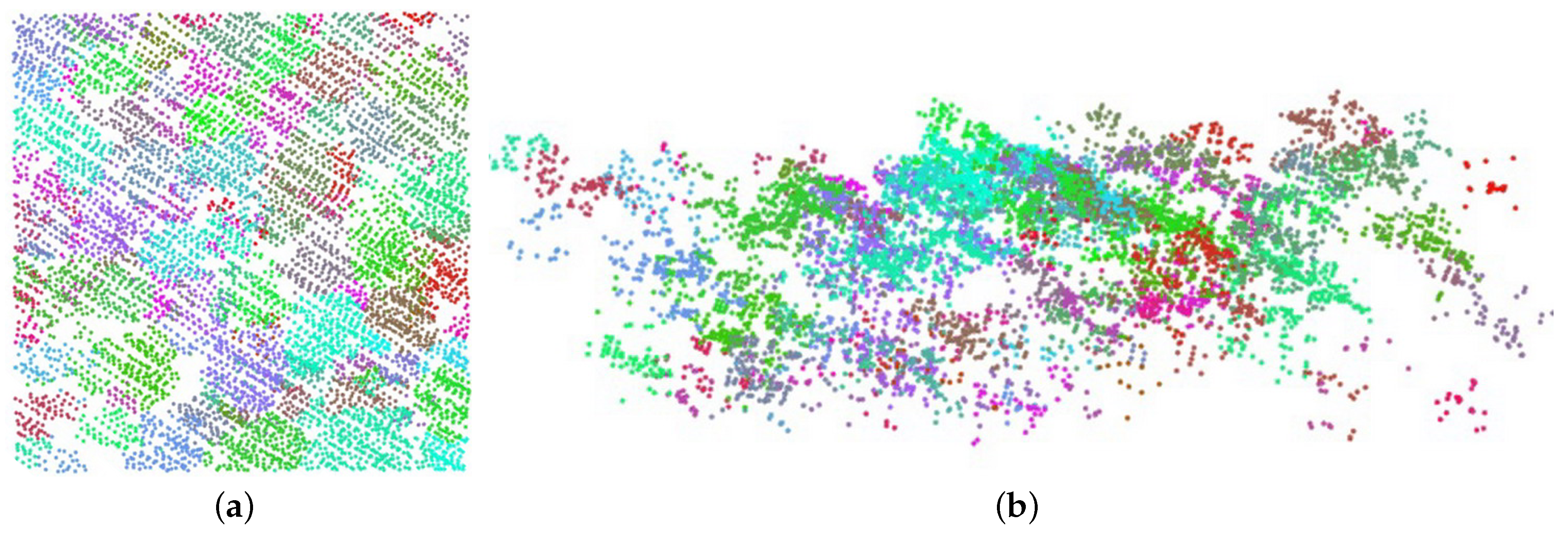
Clustering results are presented to validate the effectiveness of the above described adaptive mean shift scheme.
Figure 6 shows two different views (from top and side, respectively) of a segmented point cloud in a typical subplot (DHS0201) after two round, mean, shift-based iterative computations, with spatially adjacent point clusters rendered in different colors.
3.7. Implementation
The overall mathematical processing flow depicted in
Figure 2 is performed on a C/C++ software platform for 3D point cloud data processing that we specifically developed for research purposes based on the Point Cloud Library (PCL), which is an open-source library of algorithms for point cloud processing tasks and 3D geometry processing, such as occur in three-dimensional computer vision [
30]. Generic techniques for the classification, filtering, segmentation, interpretation, modeling, and visualization of 3D point clouds are implemented with the methods and classes contained in PCL’s modules. The computing procedures for the mean shift-based clustering in two segmentation stages are accomplished by calling a C++ wrapper which implements a standard mean shift algorithm.
We have run the LiDAR data processing software on an HP workstation computer with a 2.5 GHz Intel Core i7-6700 processor, 16 GB of RAM and 512 GB of solid state drive. The time it takes to analyze a test subplot (an area of 30 m × 30 m with 8000–15,000 laser points) using this software is about 8 s. Considering that the standard mean shift algorithm’s running time increases exponentially with the size of the whole data set, if we apply the proposed adaptive mean shift-based scheme directly to a much larger forest area of 1000 m by 1000 m, the computation time will be more than 20 h, which is extremely time consuming and inefficient. Therefore, in order to improve the computational efficiency, it is necessary to divide the area of 1000 m × 1000 m into 100 plots with the same size of 120 m × 120 m, each of which includes four 10-meter-long buffer areas on four sides to counteract edge effects. With such a division process, the total computation time taken to run this mean shift algorithm for such a large area of 1000 m × 1000 m will be drastically reduced to less than 4 h.
5. Discussion
The results obtained for individual tree identification differ significantly from study to study. It is unclear how much of the variation is caused by the applied methods and how much by the forest conditions. Accordingly, it is difficult to compare our results with those reported in existing literature using different methods since the experimental scenarios (e.g., the LiDAR configuration and the forest morphology and architecture) are not exactly the same. As the effect of variability of forest conditions has a high impact on the achieved accuracy, the performance of one method versus other methods cannot be verified without testing these methods in the same forest conditions [
33]. We make a comparative analysis between our proposed method and three typical point cloud-based methods, as well as a conventional CHM-based method, using the same data sets acquired in the study area. Obviously, the CHM-based method produces lower detection accuracy than point-based methods because it works on a raster surface model derived from the raw point cloud that always includes loss of information during transformation, but not directly on the original airborne LiDAR data that is not altered in any way. Furthermore, using the original point cloud would find the smaller trees more accurately than the traditional CHM-based methods. As shown in
Table 5, mean shift-based methods could achieve better performance for individual tree detection when compared to region growing or
k-means clustering approaches. This is mainly due to the fact that mean shift is a non-parametric algorithm, not sensitive to initializations (does not require detecting treetops) and it can handle arbitrarily shaped clusters. In order to evaluate the performance of the proposed mean shift-based method, we compare it to the similar method presented in [
17]. Our proposed new method has the similar performance with this existing method in identifying dominant and codominant trees, but can do better in detecting intermediate and suppressed trees. The mean shift algorithm described in [
17] is essentially a fixed bandwidth mean shift procedure, where a single kernel bandwidth in a specific vegetation stratum can result in obvious under-segmentations or over-segmentations. We apply a variable bandwidth mean shift algorithm, which automatically adapts the kernel bandwidth to local crown size, to reduce under- and over-segmentations. The comparison results listed in
Table 4 and
Table 5 reveal that our proposed adaptive mean shift-based method could improve the overall detection accuracy relative to standard mean shift algorithms. Ferraz et al. proposed an approach to adaptively calibrate the kernel bandwidth model required by the so-called AMS3D algorithm [
24]. However, accuracies of individual tree crown detection were not reported in [
24], and thus we cannot compare our method to it in terms of tree detection performance.
As stated in
Section 4, the tree detection accuracy can be assessed in terms of “recall” and “precision”, which are considered to be indices for commission error and omission error respectively. The commission errors usually result from over-segmentation that implies segmenting a single tree into several segments, whereas under-segmentation of tree crowns will lead to omission errors. The two types of errors are due to both the inability of the airborne LiDAR to characterize tree crowns and the detection or extraction algorithm itself. According to [
33], the LiDAR point density at which the crowns are sampled, has an impact on the identification of individual vegetation features. Misclassifications may happen where the canopy is unequally sampled by the laser pulses, but this problem can be reduced by increasing the point density [
3]. An average laser point density of 15 pt/m
used in this study is enough to capture the 3D spatial structure of individual tree crowns. When the LiDAR point density is not an issue, it is confirmed that the extraction or detection method is the main factor impacting achieved accuracy [
33].
The main problem encountered when using mean shift-based clustering algorithms to detect tree crowns is omission and commission errors, that is, such a kind of segmentation methods tends to under-detect or over-detect individual trees. Omission errors are more prone to happen than the commission ones. The main reason is that inadequate tree finding capability inherent in these methods will result in missing of trees, especially small trees. Besides, due to overlapping point cloud patches caused by complex terrain, closed forest canopies or other reasons, groups of trees standing very close to each other, identified as several single trees in the field inventory, might be treated as one cluster composed of all of these trees while performing the mean shift algorithm to segment the LiDAR point cloud. As for our proposed method, the uncertainty in tree segmentations mainly derives from the kernel bandwidth that is adapted to the estimated value of crown diameter, and estimation errors will influence the detection performance. Thus, a more sophisticated adaptive selection scheme for the kernel bandwidth might be developed to further improve the detection accuracy. Also, in dense forests with complex forms, object-oriented and shape-related rules should be utilized to improve the degree of discrimination between trees. We plan to address these issues in future work.


