An Empirical Ocean Colour Algorithm for Estimating the Contribution of Coloured Dissolved Organic Matter in North-Central Western Adriatic Sea

Abstract

The performance of empirical band ratio models were evaluated for the estimation of Coloured Dissolved Organic Matter (CDOM) using MODIS ocean colour sensor images and data collected on the North-Central Western Adriatic Sea (Mediterranean Sea). Relationships between in situ measurements (2013–2016) of CDOM absorption coefficients at 355 nm (a_CDOM355) with several MODIS satellite band ratios were evaluated on a test data set. The prediction capability of the different linear models was assessed on a validation data set. Based on some statistical diagnostic parameters (R², APD and RMSE), the best MODIS band ratio performance in retrieving CDOM was obtained by a simple linear model of the transformed dependent variable using the remote sensing reflectance band ratio R_rs(667)/R_rs(488) as the only independent variable. The best-retrieved CDOM algorithm provides very good results for the complex coastal area along the North-Central Western Adriatic Sea where the Po River outflow is the main driving force in CDOM and nutrient circulation, which in winter mostly remains confined to a coastal boundary layer, whereas in summer it spreads to the open sea as well.

1. Introduction

Ocean colour imagery collected over the past decades from many satellites has the potential for providing synoptic retrievals of bio-optical properties in the world’s oceans [1,2]. Unfortunately, the optical complexity of coastal waters affects remote sensing products and their accuracy. Thus, the pressing need of validating large-scale remote sensing coastal products makes attractive the availability of cross-site consistent in situ observations performed applying comprehensively assessed and standardized measurement protocols. Improving retrievals of water borne constituents in coastal systems requires the optimization of algorithms using regional in situ measurements of optical and biogeochemical water properties.

In this context, the Coloured Dissolved Organic Matter (CDOM) represents the optically active fraction of DOM in natural waters and plays various roles in physical and biogeochemical processes. CDOM absorption is characterized by an exponential absorption decrease from ultraviolet (UV) to visible wavelengths. It can dominate the inherent light absorption at the blue wavelengths in surface waters of the coastal seas (20%–70% at 440 nm; [3,4]), pelagic seas and oceans (>50% at 440 nm; [5]), hence competing with phytoplankton for photosynthetically active radiation [6,7]. In many coastal areas, CDOM absorption is several times that of chlorophyll and confounds the retrieval of the latter from ocean colour satellite observations due to overlapping absorbance spectra at the blue wavelengths [8,9,10]. Furthermore, CDOM has proven to be a useful tracer not only for carbon but also as a proxy for mixing in a wide variety of environments [11,12,13].

Primary sources of CDOM are rivers and groundwater near coastlines, which carry CDOM primarily from soils, but coastal waters, can contain plankton-derived CDOM produced in rivers and estuaries, as well as anthropogenic compounds from runoff, sewage discharge and other effluents [14,15]. However, biological processes such as phytoplankton growth, zooplankton grazing and microbial activity can also contribute to marine-derived CDOM in continental margins and pelagic ocean [16,17,18,19]. On the other hand, photobleaching is the dominant process for CDOM removal from natural waters [20], while microbial decomposition is of less importance [21,22]. The balance between sources and sinks controls the patterns of CDOM distribution.

Historically, many ocean colour algorithms have been developed to retrieve biogeochemical properties (e.g., chlorophyll-a, total suspended matter and CDOM) based on direct empirical relationship with the remote sensing reflectance, R_rs(λ), or ratios of R_rs at various wavelengths. Many of these models estimate the absorption coefficient of CDOM (a_CDOM) and detrital (non-pigmented) particles as a single parameter (a_CDM), because CDOM and detritus have similar spectral responses in the visible spectrum [23,24,25,26,27,28,29,30,31,32,33]. The retrieval of a_CDM by these algorithms yields reasonable results in open ocean regions. However, such algorithms typically do not work well in coastal waters due to the optical complexity of turbid coastal waters (high levels of CDOM, coloured detrital particles, and phytoplankton; [34]).

During the last years, many authors [32,35,36] have attempted to separate a_CDOM from a_CDM and to derive the CDOM spectral slope in various spectral regions [37,38,39]. Other authors [34,40] described how retrievals of bio-optical properties with a spectral references band near 640 nm showed significant improvement over the standard 555 nm band because total light absorption near 640 nm is primarily greatest for seawater itself rather than for other constituents in the water column. Anyway, the primary limitation to rigorous validation is the lack of sufficient data of coincident field measurements and satellite observations that are independent from the data used to develop the algorithms.

Satellite ocean colour optical sensors currently operating are: (a) SEVIRI (Spinning Enhanced Visible and Infrared Imager) onboard the Meteosat Second Generation (MSG-3; 2005-present) geostationary platforms with a Ground Sampling Distance (GSD) of 1–4 km; (b) Moderate Resolution Imaging Spectroradiometer on board the polar-orbiting Terra/Aqua satellites (MODIS-A; 2002–present) and the Visible Infrared Imager/Radiometer Suite (VIIRS; 2011–present) on the NPOESS Preparatory Project (NPP) satellite mission, with a GSD of 250–1000 m; (c) the Operational Land Imager (OLI; 2013–present) on the polar-orbiting Landsat-8 satellite with a GSD of 30 m; and (d) Sentinel-2A (launched on 23 June 2015) and Sentinel 3A (launched on 16 February 2016 and available from 17 November 2016) polar-orbiting multispectral high-resolution imaging ESA missions (Copernicus Services) with a GSD of 10–300 m. The data recorded by these satellite optical sensors cover the range of temporal (15 min to 15 days) and spatial (10 m to 4000 m) resolutions that are currently free available for the monitoring of sea surface dynamics.

In this study, we evaluate and analyse the performance of the MODIS-A-derived CDOM estimations using the Copernicus Marine Environment Monitoring Service CMEMS Remote sensing reflectance (R_rs at wavelengths of 412, 443, 488, 531, 547 and 667 nm) for the North-Central Western Adriatic Sea (NCWAS) in Italy, which is a complex system influenced by the Po River, one of the largest Mediterranean rivers [41]. Ocean colour satellite retrievals of a_CDOM could have many potential applications and in this work, some regional CDOM empirical algorithms for the NCWAS were tested and validated on MODIS-Aqua-measured R_rs(λ) and a_CDOM in situ data were collected from 2013 to 2016. After validation, the optimal model was used to produce a_CDOM maps of the NCWAS to describe his distribution throughout the basin. The results of the work are drawn from field measurements supported by multiple research projects in order to collect sufficient coincident satellite data with field observations.

2. Materials and Methods

2.1. Study Site

The North Adriatic Sea (Figure 1) is the northernmost part of the Mediterranean Sea, extending as far North as 45°47′N. The area is strongly influenced by river floods [42,43,44,45], which affect both the circulation through buoyancy input and the ecosystem by introducing a large amount of matters [46,47,48]. The Po River provides the major buoyancy flux with an annual mean freshwater discharge rate of about 1500 m³·s⁻¹ [41,49]. On the annual basis, the Po River alone carries 28% of the total Adriatic Sea runoff (5500−5700 m³·s⁻¹), 45% comes from the eastern coast (about half of which from Albania), 19% from the northern coast and 8% from the entire western coast [41,50]. The southward coastal flow, i.e., the Western Adriatic Current (WAC [50,51,52,53]), is driven by the Po River buoyancy flux (low-salinity waters) and northeastern Bora winds that characterize this region during the winter months. Bora winds cause elevated sea surface height along the western coasts, producing the downwelling and transport of coastal dense waters toward the open sea [54].

The Po River freshwater may flow southward along the shelf strengthening the Western Adriatic Current (WAC) or cross the shelf extending toward Istria in the central basin [55]. In particular, during periods of weak stratification, in absence of wind forcing, vortices constrain fresh Po River waters to a southward flow along the Italian shelf [56]. In contrast, in periods of stratification, particularly in spring and summer, the Po River fresh water plume spreads across the basin to the Istrian coast to form a front that divides the northern basin [57,58]. The extent of Po riverine flow and wind forcing, therefore, modulate fresh water penetration in the North Adriatic [59].

Eutrophication, which periodically occurs along the Italian coast of the Adriatic Sea [60,61,62,63], is mainly caused by the discharge of organic and inorganic matter from the Po River and detrital coming from other rivers flowing into the NCWAS and contributes to make this area a complex optical system due to simultaneous presence of CDOM, coloured detrital particles, and phytoplankton [34]. Therefore, in this work, only CDOM-based algorithms (a_CDM-based algorithms works better for other study sites where detrital particles concentrations are not so high) were considered, as CDOM is the variable of main interest for the study area; moreover, detrital particles and phytoplankton were not measured as extensively as CDOM.

2.2. Field Measurements of Seawater

As part of numerous national and international projects, several oceanographic cruises in NCWAS were conducted between November 2013 and July 2016. One hundred seventy-two water samples, corresponding to clear-sky days during which MODIS-A satellite has acquired images over the selected study area, were collected (Figure 1;

Table 1. List of field data from cruises for the absorption coefficient of Coloured Dissolved Organic Matter (a_CDOM) and salinity (S).

Region	Cruise	Dates	No. of Measurements
			aCDOM, S
Zone A	Ritmare A	29 November 2013	6
Zone B	ANOC14_1	13 February 2014	4
Zone B	ANOC14_2	21 Marh 2014	5
Zone A	Balmas 1	25 March 2014	3
Zone B	Balmas 2	24 May 2014	4
Zone B	Balmas 3	21–22 August 2014	3
Zone C	Ecosee/a 1	26 August 2014	15
Zone A	ANOC_4	22 September 2014	7
Zone C	Ecosee/a 2	7 October 2014	6
Zone B	Ecosee/a 3	17 October 2014	4
Zone B	Balmas 4	29 October 2014	3
Zone A	Ritmare B	11–12 December 2014	18
Zone B	ANOC15_1	11 February 2015	6
Zone B	ANOC15_2	14 March 2015	4
Zone B	ANOC15_2	6 May 2015	5
Zone B	Ecosee/a 4	22 July 2015	11
Zone B	ANOC15_4	18 September 2015	7
Zone B	Escavo AN	10 November 2015	10
Zone A	Solemon2015	29 November 2015	2
Zone B	ANOC16_1	11 February 2016	7
Zone B	ANOC16_2	18–19 March 2016	15
Zone A	Ritmare C	28–29 April 2016	7
Zone B	ANOC16_4	18 June 2016	6
Zone A	Medias2016	23 June 2016	6
Zone C	Post-Ecosee/a	15 July 2016	8

). For each of these water samples, CDOM and salinity were measured at the sea surface level (in situ CDOM).

Salinity (S) of the surface waters was measured using a SeaBird Electronics 911-plus CTD (Conductivity Temperature Depth). The CTD data were processed according to UNESCO standards [64].

Seawater samples for analysis of CDOM absorbance spectra were filtered through sterile Whatman GD/X 0.2 µm filters, under low pressure. The filters were washed with 100 mL of sample before its collection in order to avoid any CDOM contamination. Samples were: (a) filtered immediately after the sampling in order to avoid alteration due to microbial activity; (b) collected in amber glass bottles, previously acid-soaked (10% HCl); (c) rinsed with Milli-Q water; and (d) rinsed three times with the sample before its collection. The filtered water was kept at 4 °C until the optical measurements were performed, at the latest within four weeks.

CDOM absorbance was measured throughout a dual beam UV-VIS spectrophotometer (SHIMADZU 2600 Series), using a 10 cm path length cells with ultraviolet oxidized Milli-Q water as the blank and reference [65]. Instrument scan settings were as follows: 250–750 nm wavelength scan range, fast scan speed; 1 nm sampling interval; 0.5 nm slit width. The quartz cuvettes for blanks and samples were acid-soaked for one hour and then rinsed with Milli-Q water and sample aliquots. The absorbance (A) was converted into absorption coefficients (a_CDOMλ) by Equation (1):

a_CDOMλ = 2.303 × A_λ/L

(1)

where A_λ is the absorbance at wavelength λ and L is the path length expressed in meters. Before determining a_CDOMλ, absorbance data were corrected by subtracting the mean absorbance from 680 to 690 nm from each wavelength. The absorbance measurements ranged from 250 to 450 nm representing wavelengths where the signal was sufficiently high for a reliable estimation of a_CDOMλ [48,66]. Specifically, the absorption coefficients at 355 nm (a_CDOM355) were calculated because this wavelength shows the maximum excitation for humic-like substances [66], i.e., those of terrestrial origin. Since the NCWAS is an area impacted by high river discharges we chose this absorption coefficient for the retrieval algorithms on the assumption that most of CDOM is of terrestrial origin.

2.3. Satellite Data and Processing

MODIS-Aqua data over the study areas in the NCWAS were acquired from CMEMS online catalogue [67]. MODIS is an ocean colour sensor aboard the polar-orbiting Aqua (MODIS-A) and Terra (MODIS-T) satellite platforms with 36 spectral bands and three spatial resolutions of 250 m, 500 m and 1 km. For the Mediterranean Sea, R_rs and diffuse attenuation coefficient of light at 490 nm is operationally produced and uploaded on the CMEMS catalogue by the Group for Satellite Oceanography (GOS-ISAC) of the Italian National Research Council, in Rome, for near real time data from MODIS-A and NPP-VIIRS sensors [1,68,69].

R_rs(λ) is the fundamental quantity to be derived from ocean colour sensors and it is defined as the ratio of upwelling radiance and downwelling irradiance at any wavelength that can be expressed as the ratio of normalized water leaving radiance and the extra-terrestrial solar irradiance. The spectral remote-sensing reflectance R_rs is defined as [70]:

$$R_{rs}\left(\mathsf{\theta },\mathsf{\varphi },\mathsf{\lambda }\right)=\frac{L_w\left(\mathrm{in}\mathrm{air},\mathsf{\theta },\mathsf{\varphi },\mathsf{\lambda }\right)}{E_d\left(\mathrm{in}\mathrm{air},\mathsf{\lambda }\right)}$$

(2)

where the depth argument of “in air” indicates that R_rs is calculated using the water-leaving radiance L_w and E_d in the air, just above the water surface. The R_rs is a measure of how much of the downwelling radiance that is incident onto the water surface in any direction is eventually returned through the surface into a small solid angle $\mathsf{\Delta }\mathsf{\Omega }$ centered on a particular direction $\left(\mathsf{\theta },\varphi \right)$. However, R_rs is usually computed for nadir-viewing directions only.

In this study, nominal MODIS-A six R_rs bands (412, 443, 488, 531, 547 and 667 nm) were used for CDOM retrieval, with a spatial resolution of 1.1 km and acquired in the same dates of the field campaign period 2013–2016 (temporal window between satellite overpass and the time of field sampling = ±12 h). Figure 2a shows an example of R_rs MODIS imagery (R: 547 nm; G: 488 nm; B: 443 nm) resized on the Adriatic Sea in Italy centred on the Ancona coastal area (red box in Figure 2a). MODIS R_rs imagery was acquired on 22 July 2015, i.e., on the same date of the eleven measurement stations performed in these coastal areas (white dots in Figure 2b; Ecosee/a 4 Cruise). In Figure 2c the graph shows the R_rs spectra relative to the eleven coastal measurement stations. As expected, R_rs spectra relative to stations 3, 10 and 11 show higher values in the blue band at 443 nm. This is also evident from the MODIS R_rs RGB imagery in Figure 2 that shows both the CDOM gradient along the coastal area occurring in this date of acquisition (22 July 2015) and the higher values in the blue band at 443 nm for the stations more distant from the coast (i.e., 3, 10 and 11).

2.4. CDOM Models

Due to the lack of coincident in situ measurements and satellite observations, previous attempts to retrieve bio-information from satellite data in this complex optical region found better results on the retrieval of chlorophyll and suspended matter rather than of CDOM [71,72,73,74]. Having a consistent number of in situ and satellite data, the main aim of this work is on the definition of empirical models useful to effectively retrieve a_CDOM355 values using the optical satellite data acquired on the northwestern Adriatic coastal sea waters. Simple linear algorithms were chosen among several algorithms available in literature for CDOM retrieval, as they proved to be nearly effective with respect to the more complex models in CDOM retrieval [39]. On the other hand, empirical algorithms are known to be valid only regionally as they are particularly sensitive to changes in the specific composition of water constituents when boundary conditions are changed [75]. For the fitting and evaluation of our empirical models, the collected data were divided into two data sets: data collected from November 2013 to May 2015 (test data set, 93 observations) and data collected from July 2015 to July 2016 (validation data set, 79 observations). The initial data set was split according to two different time intervals in order to assess the prediction capability of the models. The spatial coverage of the two data sets was about the same, Figure 1. Even if the spatial coverage could be considered not very extensive, it must be kept in mind that this limitation was due to the necessity to have corresponding data from in situ and satellite measurements. The mathematical models were fitted on the test data set and the prediction performance evaluated on the validation data set. In all cases, a least squares analysis was carried out in order to identify the best relationship between the dependent variable, the CDOM absorption coefficient a_CDOM355, and the independent variables. As independent variables, the following MODIS R_rs band ratios were considered: (a) R_rs(547)/R_rs(412); (b) R_rs(547)/R_rs(488); (c) R_rs(667)/R_rs(412); (d) R_rs(667)/R_rs(488); (e) R_rs(667)/R_rs(443); and (f) R_rs(531)/R_rs(412). The inverse band ratios (a) and (b), i.e., R_rs(412)/R_rs(547) and R_rs(488)/R_rs(547), were used to define empirical algorithms in coastal waters by many authors [23,37,39,76]. However, the reference wavelength at 547 nm is affected by particles light scattering [77] that in coastal waters interferes with the CDOM retrieval. Since the NCWAS is strongly influenced by freshwaters/terrestrial input, a wavelength in the red or near infrared (667 nm) was added as numerator of the band ratios (c) and (d) in order to reduce the effects of detritus particles, as suggested by other authors [40,78,79]. At first, a simple multilinear model was tested by ordinary least square (OLS) using both the dependent and the independent variables transformed according to the log function [39]. This first analysis provided a quite low value of the adjusted coefficient of determination (adjusted R² = 0.5671). Therefore, we started using a simple multilinear model with untransformed variables and, as shown in the Results Section, proceeded according to model check and diagnostics. Once obtained some final models, their prediction capability was assessed against the validation data set.

The accuracy of model prediction was evaluated according to the following statistical indicators: (a) the adjusted coefficient of determination (adjusted R²) between the in situ validation values a_CDOM355_is’s and the calculated values a_CDOM355_c’s; (b) the mean and standard deviation of the absolute per cent difference (APD) (APD = 100 × |a_CDOM355_is − a_CDOM355_c|/a_CDOM355_is); and (c) the root mean square error (RMSE) between a_CDOM355_is’s and a_CDOM355_c’s. All the statistical analyses were performed using the open source statistical software R ver. 3.3.1 [80] at a significance level of 0.05.

Finally, the retrieved optimal model was used to construct CDOM time maps for this geographical area to further evaluate the applicability of the a_CDOM355 algorithm. These maps were then compared with the corresponding Po river discharges, which as aforementioned has a great influence in CDOM and nutrient circulation in the northwestern Adriatic Sea coastal areas.

3. Results

3.1. Field Distribution of CDOM

The surface distribution of salinity and CDOM (a_CDOM355) are summarized in

Table 2. Mean and standard deviation (s.d.) of in situ a_CDOM355 and salinity (S) measurements as a function of the area, see Figure 1. The last column shows the number of observations (n).

Region	aCDOM355 (m−1)		S		n
	Mean	s.d.	Mean	s.d.
Zone A	0.81	0.49	31.75	5.25	42
Zone B	0.38	0.30	36.27	2.26	99
Zone C	0.38	0.16	35.16	0.52	29

. Because of the complexity of the basin, the NCWSA was divided in three sub-areas: the northern part (Zone A), directly influenced from Po River runoff, and the central (Zone B) and southern parts (Zone C) both influenced by minor river discharges and indirectly by Po River runoff carried out along the northwestern Adriatic coastal areas by the WAC.

River discharges along the Western Adriatic Sea coastal areas enrich seawater in CDOM, especially in Zone A (Figure 1). A strong linear relationship between a_CDOM355 and salinity confirms this assumption (R² = 0.80; Figure 3). Salinity is a useful parameter commonly used to characterize the main terrestrial origin of CDOM, i.e., riverine CDOM, along the NCWAS.

The NCWAS is characterized by a decrease of CDOM from north to south and from coast to off-shore coupled with a salinity increase as expected. Throughout the study period a wide range of CDOM and salinity (S) are observed (S ranges from 18 to 38.7 and a_CDOM355 from 0.08 to 2.18 m⁻¹), as shown by the high standard deviations (Table 2). The high spatial and temporal variability of the data is however useful for satellite observation in order to define a properly CDOM retrieval algorithm.

3.2. Model Definition

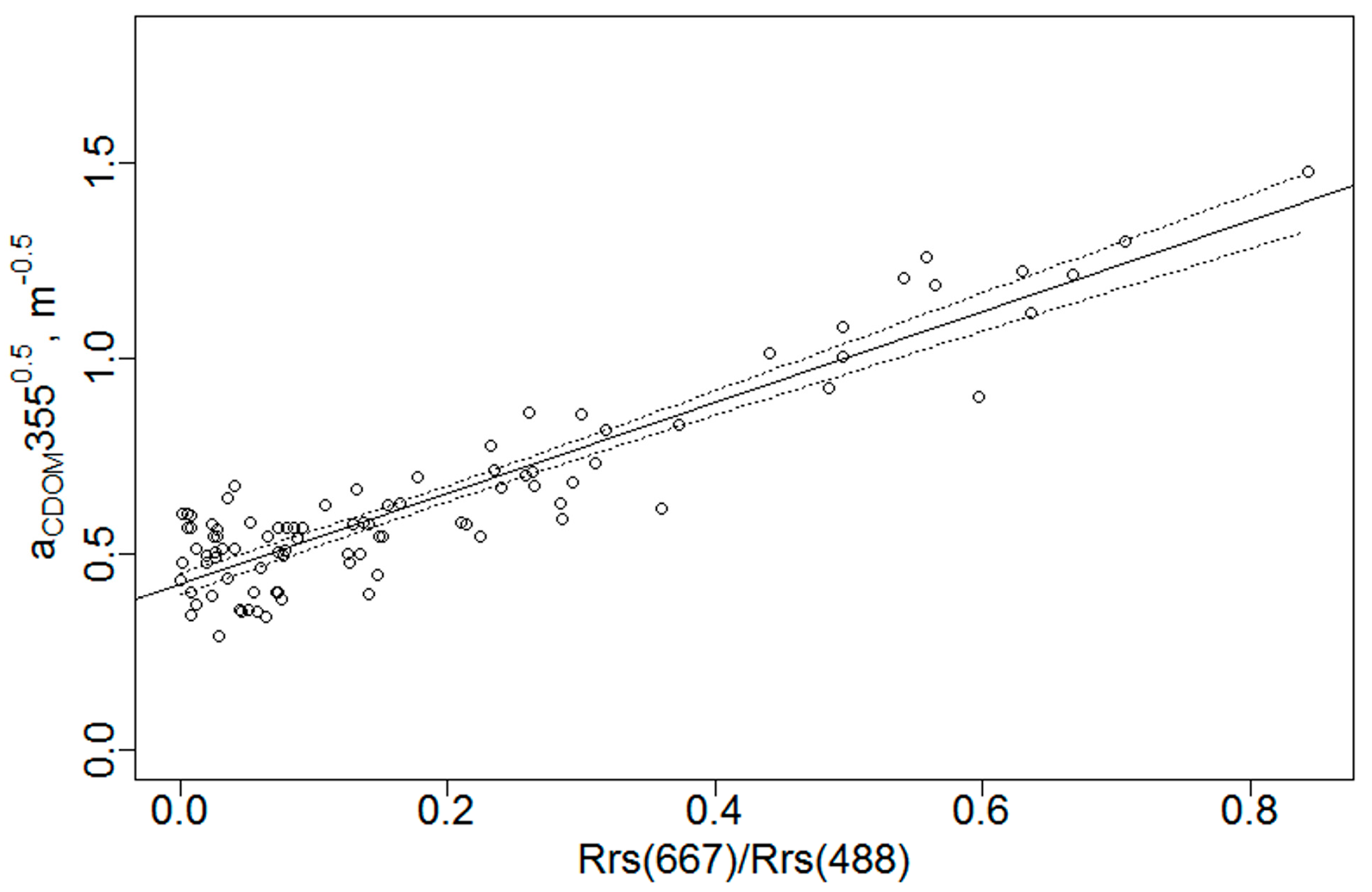
3.2.1. Simple OLS Linear Regression

Before starting the model tuning, a simple correlation analysis was carried out among the independent variables, i.e., the band ratios, to avoid the problem of collinearity. It turned out that the band ratio R_rs(667)/R_rs(443) was nearly perfectly correlated with the band ratio R_rs(667)/R_rs(488), Pearson correlation coefficient = 0.991, and the band ratio R_rs(531)/R_rs(412) was nearly perfectly correlated with the band ratio R_rs(547)/R_rs(412), Pearson correlation coefficient = 0.996. Since the aim of this work is the development of a good prediction algorithm for the dependent variable [81], the band ratios R_rs(667)/R_rs(443) and R_rs(531)/R_rs(412) were dropped in the following analysis. According to [78], the band ratio R_rs(667)/R_rs(488) was maintained because riverine CDOM still shows significant absorption at 488 nm, whereas chlorophyll does not. The band ratio R_rs(547)/R_rs(412) was maintained in order to compare our results to previous works [23,37].

At the beginning, a simple multilinear model with untransformed variables was chosen as starting algorithm:

a_CDOM355 = b₁ + b₂ × R_rs(547)/R_rs(412) + b₃ × R_rs(667)/R_rs(412) + b₄ × R_rs(667)/R_rs(488) + b₅ × R_rs(547)/R_rs(488),

(3)

where the b_i’s are the parameters to be estimated using satellite R_rs band ratios and the in situ a_CDOM355 values (test data set, 93 observations collected from November 2013 to May 2015). The results of the OLS regression for this model on the test data set are briefly summarized in

Table 3. Results of the OLS regression of a_CDOM355 algorithm (3) on the test data set.

Parameter	Parameter Estimate	Standard Error	t-Value	p
b1	0.22966	0.08290	2.770	0.006831 *
b2	0.01374	0.03707	0.371	0.711856
b3	0.26675	0.24283	1.098	0.274996
b4	1.63251	0.47735	3.420	0.000951 *
b5	−0.18052	0.15756	−1.146	0.255012

* Significant at p = 0.05.

. The adjusted coefficient of determination R² of this model was 0.8502.

From Table 3, only the intercept and the band ratio R_rs(667)/R_rs(488) can be considered significant for the model. Therefore, the following simplified algorithm (Model 1) was evaluated:

Model 1: a_CDOM355 = b₁ + b₂ × R_rs(667)/R_rs(488) by OLS.

(4)

The regression analysis of Model 1 provided the results presented in

Table 4. Results of the OLS regression of Model 1 on the test data set.

Parameter (Model 1)	Parameter Estimate	Standard Error	t-Value	p
b1	0.1165	0.0226	5.157	1.46 × 10−6 *
b2	1.9089	0.0857	22.273	<2 × 10−16 *

* Significant at p = 0.05.

. The Model 1 fit is shown in Figure 4 along with the experimental data. The adjusted coefficient of determination R² was 0.8433. This high value of adjusted R² is comforting to pursue further the simple linear model.

The diagnostic check of Model 1 was carried out according to the normal distribution of the residuals and the constancy of the variance (i.e., the homoscedasticy). The Shapiro–Wilk normality test on the model residuals gave a P value of 0.7093. However, as shown in Figure 5, the plot of the residuals against the fitted values displays a variance which increases with the increment of the fitted value (i.e., the heteroscedasticity). Heteroscedasticity was also confirmed by the studentized Breusch–Pagan test [82], which gave a p-value of 1.091 × 10⁻⁶. Besides heteroscedasticity, the residuals trend is slightly upward concave, Figure 5. This additional feature is discussed in Section 3.2.4.

Even if the OLS estimates of the parameters and the coefficient of determination (R²) are not biased by heteroscedasticity, this violation affects the confidence intervals of OLS parameters [82]. Two different approaches can be adopted to overcome heteroscedasticity. The first approach is a dependent variable transformation according to the Cox-Box analysis [83]. The second approach is to carry out a generalized least square (GLS) regression with a specific variance structure [84]. Both approaches are adopted in the following.

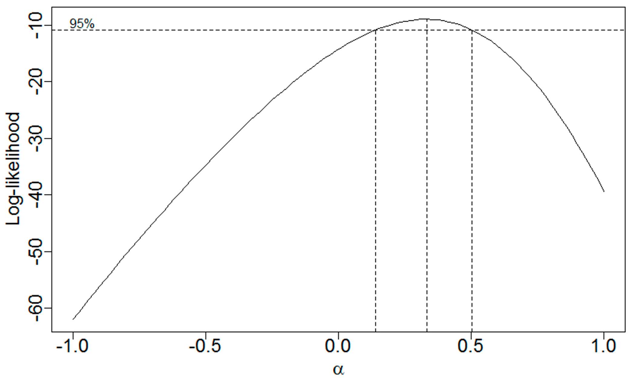
3.2.2. Dependent Variable Transformation

The dependent variable transformation was carried out according to the Box-Cox transformation, i.e., y′ = y^α, where y is the original dependent variable, y’ the transformed variable and α the transformation exponent. The plot in Figure 6, as produced by the R package MASS [85], suggests a square root transformation [83], i.e., y′ = y^0.5, with the following Model 2 to be tested:

Model 2: a_CDOM355^0.5 = b₁ + b₂ × R_rs(667)/R_rs(488) by OLS

(5)

Table 5. Results of the OLS regression of Model 2 on the test data set.

Parameter (Model 2)	Parameter Estimate	Standard Error	t-Value	p
b1	0.42387	0.01403	30.21	<2 × 10−16 *
b2	1.15761	0.05321	21.75	<2 × 10−16 *

* Significant at p = 0.05.

reports the regression results obtained for Model 2 on the test data set. The model fit is shown in Figure 7 along with the experimental data. The adjusted coefficient of determination was 0.8369.

Both the plots of the residuals (not shown) and the studentized Breusch–Pagan test (p = 0.7571) indicate that the problem of heteroscedasticity was solved.

3.2.3. Generalized Least Squares (GLS)

Another way of tackling the problem of heteroscedasticity is to perform a generalized least squares (GLS) regression analysis. In this case, the dependent and independent variables are untransformed, but the variance of the dependent variable is let to vary instead of being considered constant as in the OLS. Model 3 is, therefore, given by

Model 3: a_CDOM355 = b₁ + b₂ × R_rs(667)/R_rs(488)

(6)

with the fitting parameters b_i’s to be estimated by GLS. The fitting results of this model, which were carried out by using the R package “nlme” with a variance structure of the type “varPower()” [86], are shown in

Table 6. Results of the GLS regression Model 3 on the test data.

Parameter (Model 3)	Parameter Estimate	Standard Error	t-Value	p
b1	0.18325	0.01552	11.81	<2 × 10−16 *
b2	1.48088	0.11732	12.62	<2 × 10−16 *

* Significant at p = 0.05.

. Figure 8 shows the experimental data and the model fit. The adjusted coefficient of determination was 0.6325. Comparing the values of intercept b₁ and slope b₂ of Model 1 (Table 4) and Model 2 (Table 6), we can see that they are statistically different. This is unexpected, since heteroscedasticity should not affect the estimate of the regression parameters. Evidently, heteroscedasticity is not the only issue that emerges from the analysis of the residuals plot. In the next section, this problem is analysed more deeply.

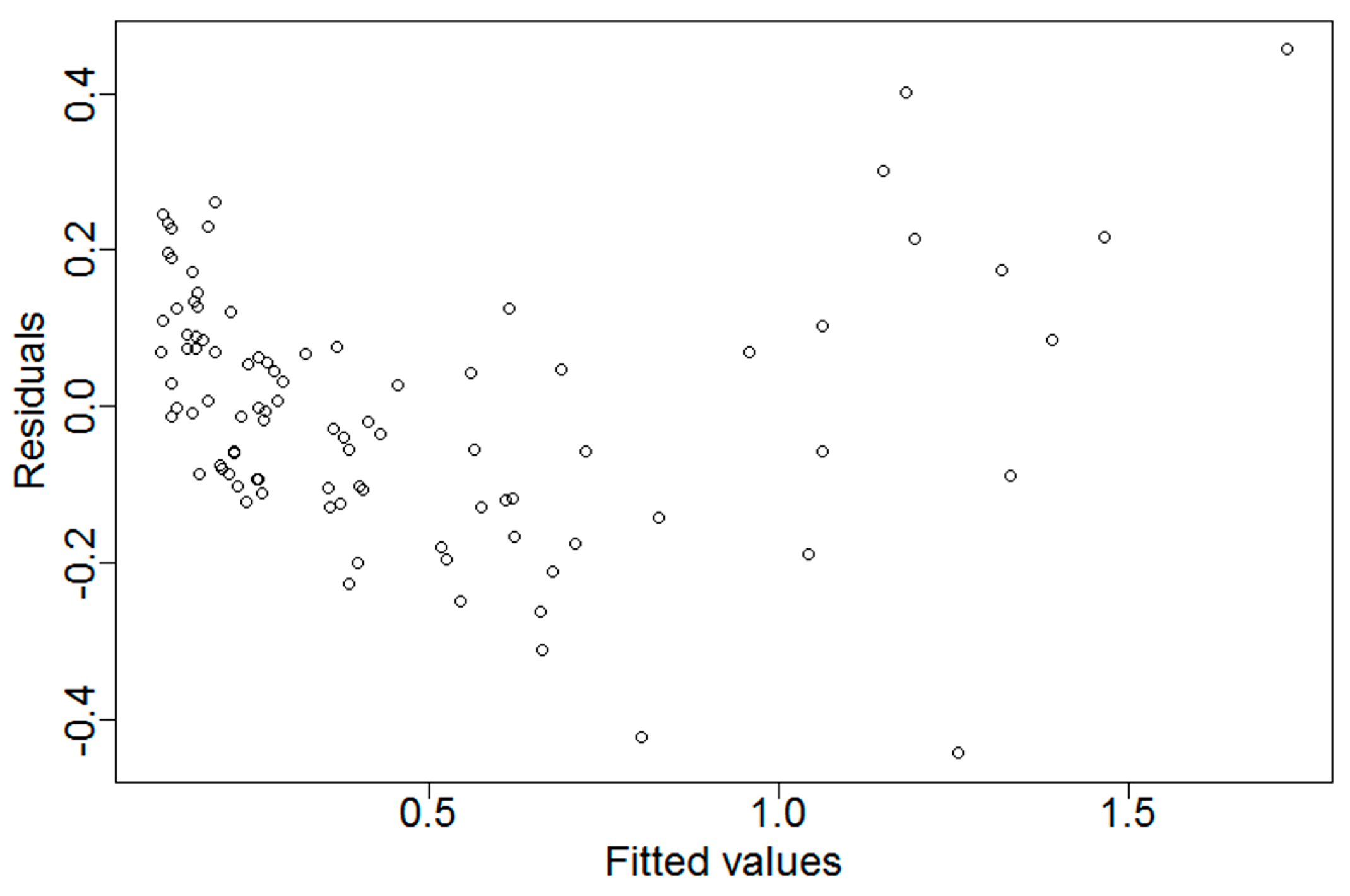
3.2.4. Curvature of the Residuals

As shown in Figure 5, a slight curved trend is present in the residuals of Model 1. This curvature usually implies the presence of higher order terms in the model [87]. In this section, besides the possibility of introducing terms of higher order, also the interaction between independent variables was considered. The detailed steps of this kind of analysis are described in Crawley [88]. According to this procedure, preliminarily to the regression analysis, two explorative investigations should be carried out: (1) a regression tree to see if the model has a complex structure, i.e., there are interaction terms between the independent variables; and (2) a generalized additive model (GAM) analysis to see if high order terms are necessary. Once ascertained the general model, a repeated OLS regression is performed cancelling, each time, the non-significant terms starting from the highest interaction terms. When all the surviving terms are significant, the regression procedure stops. However, if heteroscedasticity is present in the final model diagnostic, the regression procedure must be repeated from the beginning after the transformation of the dependent variable. In our case, the regression tree and the GAM analysis both indicated that we had to start with a model comprising all the main effects, i.e., all the independent band ratios, all the interaction terms and a quadratic term for the band ratio R_rs(667)/R_rs(488). At the end of the regression steps, the studentized Breusch–Pagan test indicated that the dependent variable had to be transformed, also in this case as y′ = y^0.5. Repeating all the regression steps, the final model was the one with the dependent variable transformed as y′ = y^0.5 and with the following lengthy form:

Model 4: a_CDOM355^0.5 = b₁ × R_rs(547)/R_rs(412) + b₂ × R_rs(667)/R_rs(412) + b₃ × R_rs(667)/R_rs(488) + b₄ × R_rs(547)/R_rs(488) + b₅ × [R_rs(547)/R_rs(412)]² + b₆ × [R_rs(667)/R_rs(412)]² + b₇ × [Rrs(667)/Rrs(488)]² + b₈ × [Rrs(547)/Rrs(488)]² + b₉ × Rrs(547)/Rrs(412) × Rrs(667)/Rrs(412) + b₁₀ × Rrs(547)/Rrs(412) × Rrs(667)/Rrs(488) + b₁₁ × Rrs(667)/Rrs(412) × Rrs(667)/Rrs(488)

(7)

The adjusted coefficient of determination R² was 0.9873. The results of the regression analysis carried out by OLS are summarized in

Table 7. Results of the OLS regression of Model 4 on the test data set.

Parameter (Model 4)	Parameter Estimate	Standard Error	t-Value	p
b1	−0.39669	0.07517	−5.277	1.05 × 10−6 *
b2	2.18707	0.74484	2.936	0.004309 *
b3	−5.50891	1.12927	−4.878	5.18 × 10−6 *
b4	1.70642	0.12586	13.55	<2 × 10−16 *
b5	0.06978	0.01424	4.901	4.74 × 10−6 *
b6	3.18145	1.13802	2.796	0.006450 *
b7	13.1729	3.34276	3.941	0.000170 *
b8	−0.74416	0.10134	−7.343	1.37 × 10−10 *
b9	−1.15771	0.27683	−4.182	7.20 × 10−5 *
b10	3.41274	0.61429	5.556	3.34 × 10−7 *
b11	−13.29309	3.88291	−3.423	0.000967 *

* Significant at p = 0.05.

.

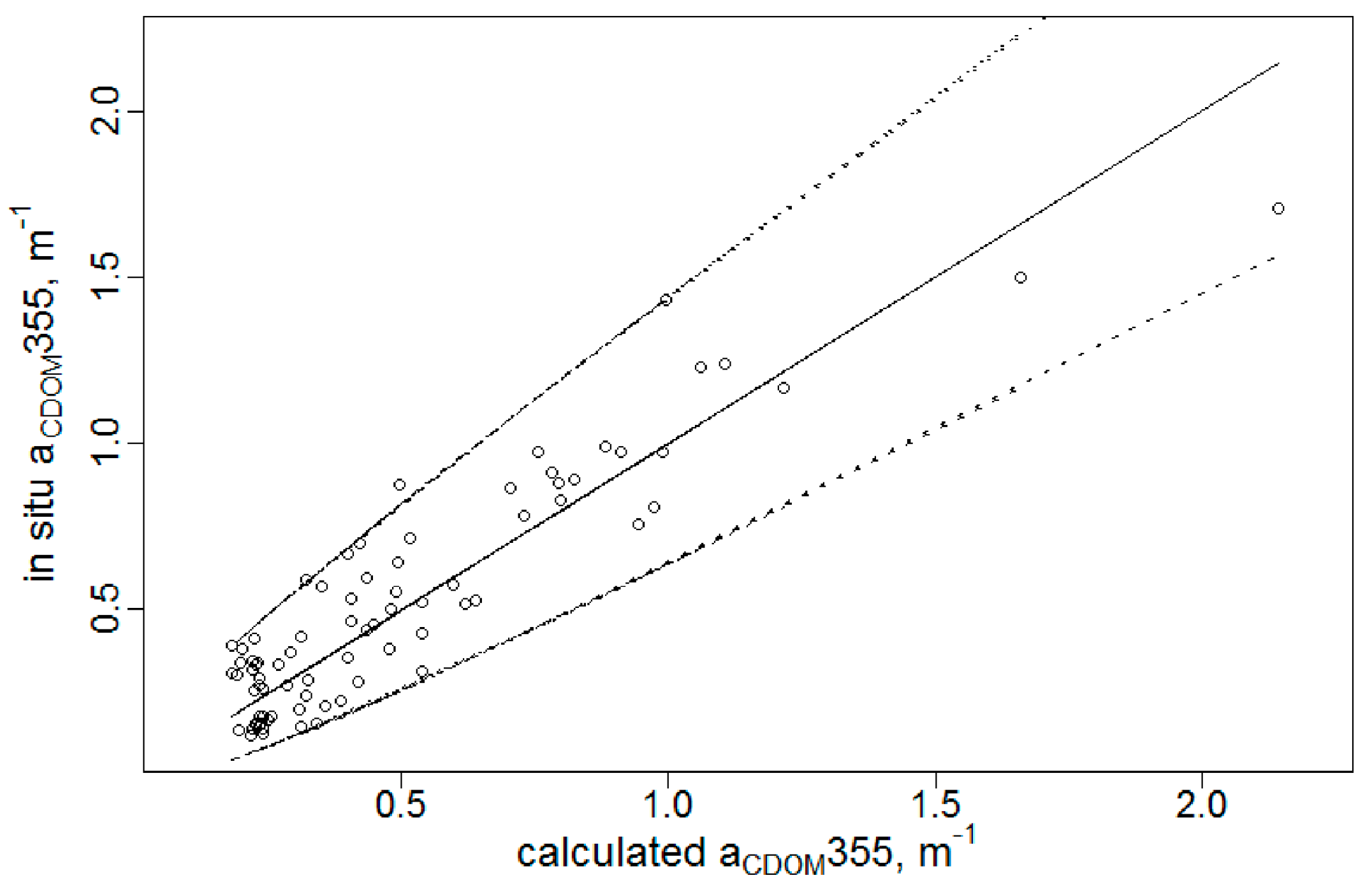
3.2.5. Model Validation

In order to validate the four models tested so far, the calculated values a_CDOM355_c of each model were compared to the in situ values of the validation data a_CDOM355_is (validation data set, 79 observations collected from 2015 to 2016). The calculated a_CDOM355_c were obtained by inserting the appropriate values of the band ratios of the validation data set into the equations of the four fitted models. The accuracy of the four models was then assessed by comparing the calculated values against the in situ values of the validation data set according to following statistical indicators: (a) the adjusted coefficient of determination (adjusted R²) between a_CDOM355_is and a_CDOM355_c; (b) the mean and standard deviation of the APD (APD = 100 × |a_CDOM355_is − a_CDOM355_c|/a_CDOM355_is); and (c) the RMSE between a_CDOM355_is and a_CDOM355_c.

Table 8. Comparison results of the prediction ability of the four models on the validation data set. Three additional models taken from bibliography are also included.

Algorithm	Adjusted R2	APD	RMSE (m−1)
Model 1	0.8426	33 (28) *	0.1421
Model 2	0.8322	31 (24)	0.1482
Model 3	0.8426	35 (31)	0.1496
Model 4	0.5528	72 (65)	0.3344
Mannino et al. [37]	0.5594	28 (23)	0.2580
Del Castillo and Miller [78]	0.0098	74 (71)	0.3541
D’Sa and Miller [76]	0.4122	39 (30)	0.2922

* Mean value (standard deviation).

summarizes the results of the validation. For comparison, we have considered three additional empirical models developed by other authors. When a band of the additional models was not coincident with any of the bands considered for this work, the closest band among those at hand was chosen.

The second column of Table 8 indicates a very good correlation between the calculated and the in situ values for the first three models, with adjusted R² values in the range of 0.832–0.843. The adjusted R² value for Model 4 was far below in spite of its highest fitting of the test data. The good agreement for the first three models must be truly appreciated considering that the validation data were collected more than one year after the test data. According to the APD values, Model 2 has the best prediction accuracy, while Model 4 the lowest one. The best value, 31 for Model 2, is comparable with APD’s found by other authors [39,71] even if Mannino et al. obtained values as low as 18–20 [37]. On the absolute scale, the prediction accuracy was almost comparable for the first three models, as indicated by the RMSE values. With the highest RMSE value, the low prediction capability of Model 4 was confirmed. The performances of the three additional models were quite low and comparable to Model 4, in some cases even worse.

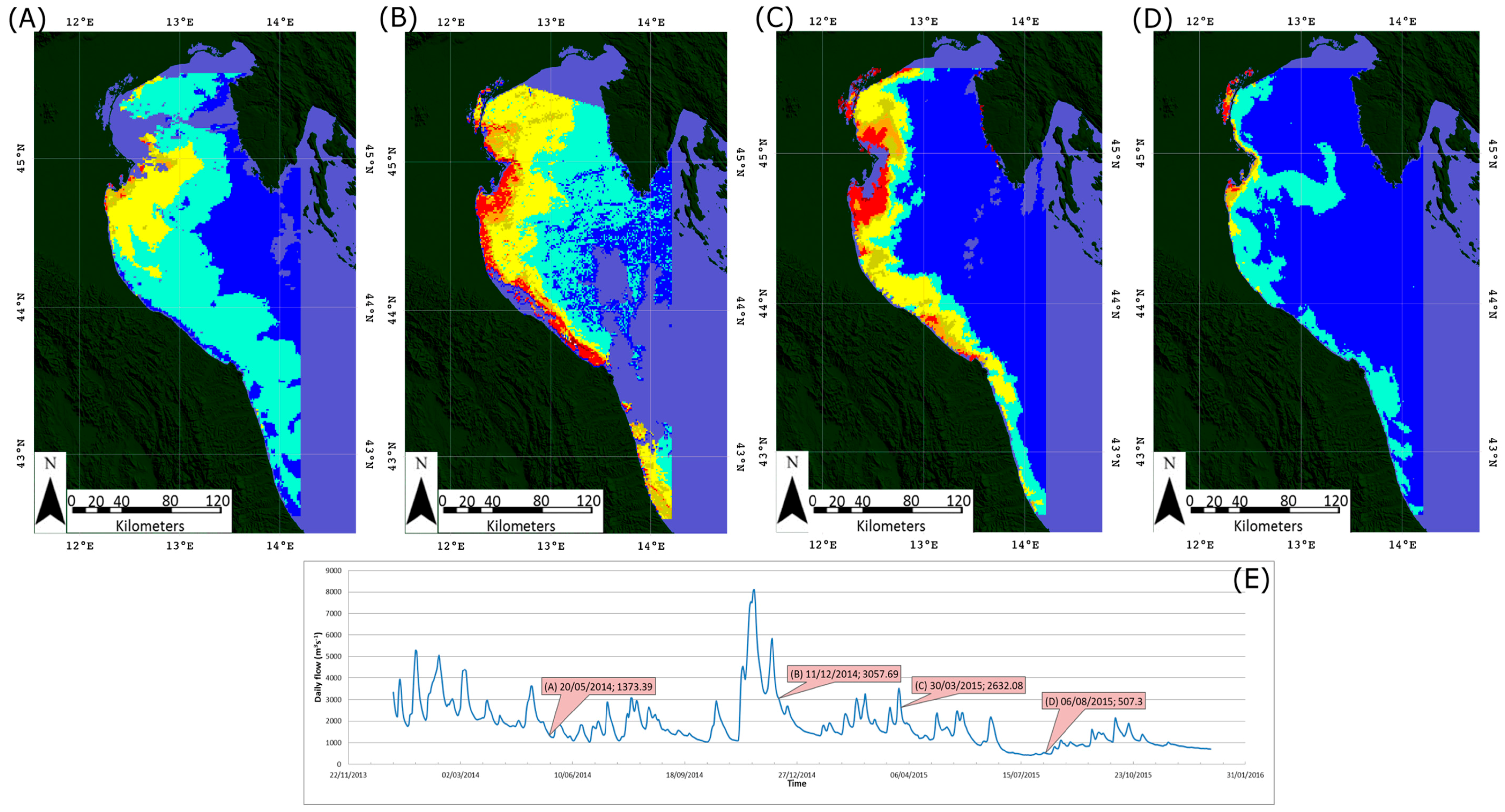
3.3. Application of Satellite-Derived CDOM

In order to verify the ability of Model 2 (i.e., the one with the best prediction accuracy) to capture the dynamic range of CDOM for the test areas, maps of satellite a_CDOM355 were produced for the studied region. The selected days to produce the maps were chosen on the basis of daily flow rate of the Po River [89] and the availability of cloud free MODIS-A R_rs imagery in order to show the distribution of riverine CDOM along the NCWAS. The processed MODIS-A satellite R_rs images, as shown as examples in Figure 9, indicate that the proposed Model 2 algorithm can be confidently applied to generate consistent MODIS-A maps of a_CDOM355. The satellite retrieved CDOM distribution fits quite well based on the field measurements and the processes that affect the distribution of biochemical properties along the NCWAS.

Furthermore, the field measurements as well as optical satellite data demonstrate a decrease in a_CDOM355 from North (Po River mouth) towards South and from nearshore to offshore. Increasing and decreasing of CDOM due to differences in Po River flow rate is a quite evident process (as expected) along the Western coast of the Adriatic Sea.

4. Discussion

According to the above model analysis, the band ratio R_rs(667)/R_rs(488) was the most significant independent variable for the retrieval of a_CDOM355 in the study area of NCWAS, which is characterized by high river discharges. The results confirm that the performance of empirical algorithms in a complex basin, i.e., a basin strongly influenced by freshwater/terrestrial input, can be significantly improved by selecting at least one band with a wavelength greater than 600 nm [34,40,78]. The additional spectral bands in the red or near infrared could be also helpful in better accounting for detritus particles because they are less sensible to the constituents in the seawater column so that the R_rs(667) can be assumed to be mainly invariant as not influenced by detritus particles. On the sea surface at the wavelength of 667 nm the total light absorption is highest for seawater rather than for other constituents in the seawater column so that the R_rs(667) can be assumed to be constant [34]. Moreover, riverine CDOM shows a higher absorption at 488 nm than the chlorophyll [40]. On the other hand, the R_rs(547) nm is mostly driven by particles light scattering that in coastal water could reduce the uncertainty of CDOM retrieval when used as a reference point in band ratios [77]. Furthermore, the NCWAS is well described by many authors to be impacted by particles coming from many rivers [60,61,62,90]. Therefore, we applied the ratio R_rs(667)/R_rs(488) that is more sensitive to changes in CDOM rather than in chlorophyll because, in low salinity waters as in the NCWAS, most of the light attenuation is controlled by CDOM [14,91]. The high river discharges on the NCWAS should therefore imply the use of a band ratio normally used in retrieving algorithms for river-plume waters. In this work, only simple linear models were considered. However, as shown in the Section 3, they proved to be quite effective for modelling the available data. Of the final four algorithms, only Model 2 and Model 4 fulfil the fundamental requirements for a correct linear regression. Considering the prediction capability, from our analysis Model 2 can be indicated as the best algorithm in order to retrieve a_CDOM355 in NCWAS starting from the band ratio R_rs(667)/R_rs(488). The predictions of this model in data collected more than one year after the model fitting showed a very good comparison with the in situ measured data with an adjusted R² value of 0.8322, Table 8. Just for comparison, similar validation analyses for coastal sea waters gave R² values of: 0.37 in the same geographical area for a_CDOM412 [71], 0.61 for a_CDOM443 in the western Canada coastal waters [92], 0.62 for a_CDOM412 in the Gulf of Mexico [91], 0.70 for a_CDOM442 in the North Sea and Western English Channel [32], 0.83 a_CDOM420 in a Finnish lake [93] and 0.96 for a_CDOM355, a_CDOM412 and a_CDOM443 in coastal waters in U.S. Middle Atlantic Bight [37]. To better illustrate the agreement between calculated and measured values, in Figure 10 a graphical comparison between the in situ validation data and the Model 2 calculated data is shown. Figure 10 indicates that the prediction capability of the model seems to be rather good. It is however fair to add that the model performances could be overestimated due to the size of the validation data set, which is not very large, and the limited range of a_CDOM355 values, which roughly spans only one order of magnitude.

Plots of satellite-derived distributions of a_CDOM355 are spatially and temporally consistent with changes in Po River discharges (Figure 9) and the NCWAS. Since terrestrial DOM is the main source of CDOM to estuaries and coastal seas, a_CDOM355 values should generally decrease from the estuary to off-shore. The CDOM maps of Figure 9, moreover, show that the minimum CDOM concentration appears in 2015 only after a long period of reduced Po River flows (daily flow less than 500 m³·s⁻¹), nevertheless determining the distribution of the sediments along the western Adriatic coast. The increase in surface a_CDOM355 corresponds to high river discharge.

As an example, Figure 9b and Figure 11 show how an exceptional Po River discharge, happened in autumn 2014 (mean discharge 10 November–10 December 2014: 5028.2 m³·s⁻¹) spreads high concentrations of riverine CDOM over the NCWAS compared with other periods, reaching the Istrian coast [44]. In particular, Figure 11 shows the CDOM map obtained by applying Model 2 to the R_rs Landsat 8 (30 m/pixel) bands closest to the R_rs(667) and R_rs(488) MODIS bands. In this case, we exceptionally tested the Model 2 equation on the Landsat R_rs imagery, which was besides the severe cloud cover affecting the study area the only available for the day of the maximum Po River discharge between 2014 and 2016 (i.e., 19 November 2014; see plot of Figure 9e). Landsat retrieved CDOM map, because of the higher GSD, moreover, correctly depicts the detrital contribution of all the minor rivers’ discharges occurring in the North and West Adriatic coasts, as well as the Venice Lagoon sub-basins. However, it is important to remark that MODIS R_rs are recursively generated as standard product [68,69], while Landsat R_rs were retrieved by applying the following commonly used R_rs equation using as input Landsat radiance data.

R_rs(λ) = L_tot(λ) − L_surf(λ)/E_d(λ) = L_w(λ)/E_d(λ)

(8)

where L_tot(λ) = L₀(λ) − L↑(λ) is the total spectral radiance signal above the water surface; L_surf(λ) is the contribution to the radiance due to the reflection of the water surface; L_w(λ) is the water leaving spectral radiance; and E_d(λ) = E(λ)cosθ_zτ_↓(λ) is the incident irradiance above the water surface. Once the surface reflection is removed, the R_rs can be considered Lambertian for short variation of the viewing angle around the zenith. In order to estimate and then remove the signal reflected by the water surface (L_surf) we used the Hydrolight 4.3 software that is a radiative transfer numerical model that computes radiance distributions and derived quantities for water bodies [94].

Landsat atmospheric correction and R_rs retrieval are anyhow out of the scope of this study and the use of Landsat data is not an important step for consistency validation of the CDOM algorithm here proposed and validated only for MODIS—A R_rs on the NCWAS coastal areas. In addition, the central wavelengths of the two bands applied for the a_CDOM algorithm (667 nm and 488 nm) from Landsat-8 and MODIS are close, while their bandwidths and SNRs (signal to noise ratio) are different.

The decrease in surface a_CDOM355 towards Southern Adriatic Sea and off-shore during spring 2014 and summer 2015 is consistent with photobleaching due to high solar radiation (both periods; [10,20]) as well as low river discharge (summer period).

5. Conclusions and Future Work

Based on the in situ data collected from several cruises in the North-Central Western Adriatic Sea (Mediterranean Sea) and on the corresponding MODIS ocean colour data, empirical models for the estimation of Coloured Dissolved Organic Matter (CDOM) using sensor data were tested. Data were split into two data sets: a test data set for model fitting (data collected from 2013 to 2015) and a validation data set (data collected from 2015 to 2016) for model assessment. The model set up was based on some statistical indicators: adjusted R², absolute percentage difference (APD) and root mean square error (RMSE).

Following statistical check and diagnostic, four final simple linear models were obtained. Three of them gave very good results in terms of comparison between the calculated and the in situ measured values of the validation data set (adjusted R² in the range 0.83–0.84). On the base of APD and RMSE, the best model resulted to be a simple linear model (Model 2) with the dependent variable transformed according to y′ = y^0.5 and the band ratio R_rs(667)/R_rs(488) as the only independent variable. The use of the R_rs(667) instead of the R_rs(547) as a reference point in band ratio seems to reduce the uncertainty of CDOM retrieval in the NCWAS characterized by high light particles scattering. However, in this view, future work will be dedicated to demonstrate that retrievals are effective even for high particulate concentrations, e.g., by showing their efficacy even for high R_rs(547) conditions and for particularly high river outflows.

The validation methods and processing of MODIS-A data show that Model 2 provides a good retrieval for a_CDOM355 and it is consistent with the spatial and temporal distribution of freshwater discharges along the Western Adriatic Sea.

The spatial and temporal limitations associated with in situ and remote sensing data has introduced some uncertainties. Anyway, the retrieved algorithm (Model 2) is very promising for CDOM mapping in this complex basin and should be considered when applying ocean colour remote sensing data to quantify other ocean constituents (e.g., chlorophyll).

MODIS-A data provision started on 2002 and its quality in terms of bands and Signal to Noise Ratio is going down, therefore, future work will be focused on developing new CDOM algorithms for the recently launched multispectral optical satellite sensors (e.g., Landsat 8 and Sentinel 2 and 3 with a GSD of 30 m) including also VIIRS observations and next generation hyperspectral sensor (e.g., EnMAP and PRISMA with a GSD of 30 m and the VNIR VENµS Superspectral Camera with a GSD of 10 m) and their validation strategy using novel in situ measurements.

References

1. Volpe, G.; Santoleri, R.; Vellucci, V.; Ribera d’Alcala, M.; Marullo, S.; D’Ortenzio, F. The colour of the Mediterranean Sea: Global versus regional bio-optical algorithms evaluation and implication for satellite chlorophyll estimates. Remote Sens. Environ. 2007, 107, 625–638. [Google Scholar] [CrossRef]
2. McClain, C.R. A decade of satellite ocean color observation. Annu. Rev. Mar. Sci. 2009, 1, 19–42. [Google Scholar] [CrossRef] [PubMed]
3. Del Vecchio, R.; Subramaniam, A. Influence of the Amazon River on the surface optical properties of the western tropical North Atlantic Ocean. J. Geophys. Res. 2004, 109, C11001. [Google Scholar] [CrossRef]
4. Pan, X.; Mannino, A.; Russ, M.E.; Hooker, S.B. Remote sensing of the absorption coefficients and chlorophyll a concentration in the U.S. southern Middle Atlantic Bight from SeaWiFS and MODIS-Aqua. J. Geophys. Res. 2008, 113, C11022. [Google Scholar] [CrossRef]
5. Siegel, D.A.; Maritorena, S.; Nelson, N.B.; Hansell, D.A.; Lorenzi-Kayser, M. Global distribution and dynamics of colored dissolved and detrital organic materials. J. Geophys. Res. 2002, 107, C123228. [Google Scholar] [CrossRef]
6. Keith, D.J.; Yoder, J.A.; Freeman, S.A. Spatial and temporal distribution of coloured dissolved organic matter (CDOM) in Narragansett Bay, Rhode Island: Implication for phytoplankton in coastal waters. Estuar. Coast. Shelf Sci. 2002, 55, 705–717. [Google Scholar] [CrossRef]
7. McKee, D.; Cunningham, A.; Jones, K.J. Optical and hydrographic consequences of freshwater run-off during spring phytoplankton growth in a Scottish fjord. J. Plankton Res. 2002, 24, 1163–1171. [Google Scholar] [CrossRef]
8. Bricaud, A.; Morel, A.; Prieur, L. Absorption by dissolved organic matter of the sea (yellow substance) in the UV and visible domains. Limnol. Oceanogr. 1981, 26, 43–53. [Google Scholar] [CrossRef]
9. Nelson, J.R.; Guarda, S. Particulate and dissolved spectral absorption on the continental shelf of the southeastern United States. J. Geophys. Res. 1995, 100, 8715–8732. [Google Scholar] [CrossRef]
10. Coble, P. Marine Optical Biogeochemistry: The Chemistry of Ocean Color. Chem. Rev. 2007, 107, 402–418. [Google Scholar] [CrossRef] [PubMed]
11. Swan, C.M.; Siegel, D.A.; Nelson, N.B.; Carlson, C.A.; Nasir, E. Biogeochemical and hydrographic controls on chromophoric dissolved organic matter distribution in the Pacific Ocean. Deep-Sea Res. I 2009, 56, 2175–2192. [Google Scholar] [CrossRef]
12. Nelson, N.B.; Siegel, D.A.; Carlson, C.A.; Swan, C.M. Tracing global biogeochemical cycles and meridional overturning circulation using chromophoric dissolved organic matter. Geophys. Res Lett. 2010, 37. [Google Scholar] [CrossRef]
13. Stedmon, C.A.; Osburn, C.L.; Gragh, T. Tracing water mass mixing in the Baltic–North Sea transition zone using the optical properties of coloured dissolved organic matter. Estuar. Coast. Shelf Sci. 2010, 87, 156–162. [Google Scholar] [CrossRef]
14. Del Castillo, C.E.; Coble, P.G.; Morell, J.M.; López, J.M.; Corredor, J.E. Analysis of the optical properties of the Orinoco River plume by absorption and fluorescence spectroscopy. Mar. Chem. 1999, 66, 35–51. [Google Scholar] [CrossRef]
15. Del Vecchio, R.; Blough, N.V. Spatial and seasonal distribution of chromophoric dissolved organic matter (CDOM) and dissolved organic carbon (DOC) in the Middle Atlantic Bight. Mar. Chem. 2004, 89, 169–187. [Google Scholar] [CrossRef]
16. Rochelle-Newall, E.J.; Fisher, T.R. Chromophoric dissolved organic matter and dissolved organic carbon in Chesapeake Bay. Mar. Chem. 2002, 77, 23–41. [Google Scholar] [CrossRef]
17. Steinberg, D.K.; Nelson, N.; Carlson, C.A.; Prusak, A.C. Production of chromophoric dissolved organic matter (CDOM) in the open ocean by zooplankton and the colonial cyanobacterium Trichodesmium spp. Mar. Ecol. Prog. Ser. 2004, 267, 45–56. [Google Scholar] [CrossRef]
18. Andrew, A.A.; Del Vecchio, R.; Subramaniam, A.; Blough, N.V. Chromophoric dissolved organic matter (CDOM) in the equatorial Atlantic Ocean: Optical properties and their relation to CDOM structure and source. Mar. Chem. 2013, 148, 33–43. [Google Scholar] [CrossRef]
19. Nelson, N.B.; Siegel, D.A. The global distribution and dynamics of chromophoric dissolved organic matter. Annu. Rev. Mar. Sci. 2013, 5, 447–476. [Google Scholar] [CrossRef] [PubMed]
20. Mopper, K.; Keiber, D.J. Photochemistry and the cycling of carbon, sulfur, nitrogen and phosphorus. In Biogeochemistry of Marine Dissolved Organic Matter; Hansel, D.A., Carlson, C.A., Eds.; Academic Press: San Diego, CA, USA, 2002; pp. 455–507. [Google Scholar]
21. Moran, M.A.; Sheldon, W.M.; Zepp, R.G. Carbon loss and optical property changes during long-term photochemical and biological degradation of estuarine dissolved organic matter. Limnol. Oceangr. 2000, 45, 1254–1264. [Google Scholar] [CrossRef]
22. Boyd, T.J.; Osburn, C.L. Changes in CDOM fluorescence from allochthonous and autochthonous sources during tidal mixing and bacterial degradation in two coastal estuaries. Mar. Chem. 2004, 89, 189–210. [Google Scholar] [CrossRef]
23. Carder, K.L.; Chen, F.R.; Lee, Z.P.; Hawes, S.K.; Kamykowski, D. Semianalytic moderate-resolution imaging spectrometer algorithms for chlorophyll and absorption with bio-optical domains based on nitrate-depletion temperatures. J. Geophys. Res. 1999, 104, 5403–5421. [Google Scholar] [CrossRef]
24. Hoge, F.E.; Wright, C.W.; Lyon, P.E.; Swift, R.N.; Yungel, J.K. Inherent optical properties imagery of the western North Atlantic Ocean: Horizontal spatial variability of the upper mixed layer. J. Geophys. Res. 2001, 106, 31129–31140. [Google Scholar] [CrossRef]
25. Lee, Z.P.; Carder, K.L.; Arnone, R.A. Deriving inherent optical properties from water color: A multiband quasi-analytical algorithm for optically deep waters. Appl. Opt. 2002, 41, 5755–5772. [Google Scholar] [CrossRef] [PubMed]
26. Maritorena, S.; Siegel, D.A.; Peterson, A.R. Optimization of a semianalytical ocean color model for global-scale applications. Appl. Opt. 2002, 41, 2705–2714. [Google Scholar] [CrossRef] [PubMed]
27. Siegel, D.A.; Maritorena, S.; Nelson, N.B.; Behrenfeld, M.J. Independence and interdependencies among global ocean color properties: Reassessing the bio-optical assumption. J. Geophys. Res. 2005, 110, C07011. [Google Scholar] [CrossRef]
28. Siegel, D.A.; Maritorena, S.; Nelson, N.B.; Behrenfeld, M.J.; McClain, C.R. Colored dissolved organic matter and its influence on the satellite-based characterization of the ocean biosphere. Geophys. Res. Lett. 2005, 32, L20605. [Google Scholar] [CrossRef]
29. Doerffer, R.; Schiller, H. The MERIS case 2 water algorithm. Int. J. Remote Sens. 2007, 28, 517–535. [Google Scholar] [CrossRef]
30. Lee, Z.P.; Arnone, R.A.; Hu, C.; Werdell, P.J.; Lubac, B. Uncertainties of optical parameters and their propagations in an analytical ocean color inversion algorithm. Appl. Opt. 2010, 49, 369–381. [Google Scholar] [CrossRef] [PubMed]
31. Bricaud, A.; Ciotti, A.M.; Gentili, B. Spatial-temporal variations in phytoplankton size and colored detrital matter absorption at global and regional scales, as derived from twelve years of SeaWiFS data (1998–2009). Glob. Biogeochem. Cycles 2012, 26, GB1010. [Google Scholar] [CrossRef]
32. Tilstone, G.H.; Peters, S.W.M.; Van Der Woerd, H.J.; Eleveld, M.A.; Ruddick, K.; Schönfeld, W.; Krasemann, H.; Martinez-Vicente, V.; Blondeau-Patissier, D.; Röttgers, R.; et al. Variability in specific-absorption properties and their use in a semianalytical ocean colour algorithm for MERIS in north sea and western English channel coastal waters. Remote Sens. Environ. 2012, 118, 320–338. [Google Scholar] [CrossRef]
33. Werdell, P.J.; Franz, B.A.; Bailey, S.W.; Feldman, G.C.; Boss, E.; Brando, V.E.; Dowell, M.; Hirata, T.; Lavender, S.J.; Lee, Z.; et al. Generalized ocean color inversion model for retrieving marine inherent optical properties. Appl. Opt. 2013, 52, 2019–2037. [Google Scholar] [CrossRef] [PubMed]
34. Aurin, D.A.; Dierssen, H.M. Advantages and limitations of ocean color remote sensing in CDOM-dominated, mineral-rich coastal and estuarine waters. Remote Sens. Environ. 2012, 125, 181–197. [Google Scholar] [CrossRef]
35. Dong, Q.; Shang, S.; Lee, Z. An algorithm to retrieve absorption coefficient of chromophoric dissolved organic matter from ocean color. Remote Sens. Environ. 2013, 128, 259–267. [Google Scholar] [CrossRef]
36. Matsuoka, A.; Hooker, S.B.; Bricaud, A.; Gentili, B.; Babin, M. Estimating absorption coefficients of colored dissolved organic matter (CDOM) using a semi-analytical algorithm for southern Beaufort Seawaters: Application to deriving concentrations of dissolved organic carbon from space. Biogeosciences 2013, 10, 917–927. [Google Scholar] [CrossRef]
37. Mannino, A.; Russ, M.E.; Hooker, S.B. Algorithm development and validation for satellite-derived distributions of DOC and CDOM in the U.S. Middle Atlantic Bight. J. Geophys. Res. 2008, 113, C07051. [Google Scholar] [CrossRef]
38. Fichot, C.G.; Kaiser, K.; Hooker, S.B.; Amon, R.M.W.; Babin, M.; Belanger, S.; Walker, S.A.; Benner, R. Pan-Arctic distributions of continental runoff in the Arctic Ocean. Sci. Rep. 2013, 3, 1053. [Google Scholar] [CrossRef] [PubMed]
39. Mannino, A.; Novak, M.G.; Hooker, S.B.; Hyde, K.; Aurin, D. Algorithm development and validation of CDOM properties for estuarine and continental shelf waters along the northeastern U.S. coast. Remote Sens. Environ. 2014, 152, 576–602. [Google Scholar] [CrossRef]
40. Zhu, W.; Yu, Q.; Tian, Y.Q.; Becker, B.L.; Zheng, T.; Carrick, H. An assessment of remote sensing for colored dissolved organic matter in complex freshwater environments. Remote Sens. Environ. 2014, 140, 766–778. [Google Scholar] [CrossRef]
41. Raicich, F. On the fresh water balance of the Adriatic coast. J. Mar. Syst. 1996, 9, 305–319. [Google Scholar] [CrossRef]
42. Marini, M.; Fornasiero, P.; Artegiani, A. Variations of Hydrochemical Features in the Coastal Waters of Monte Conero: 1982–1990. Mar. Ecol. 2002, 23, 258–271. [Google Scholar] [CrossRef]
43. Campanelli, A.; Fornasiero, P.; Marini, M. Physical and Chemical characterization of water column in the Piceno coastal area (Adriatic Sea). Fresenius Environ. Bull. 2004, 13, 430–435. [Google Scholar]
44. Campanelli, A.; Grilli, F.; Paschini, E.; Marini, M. The influence of an exceptional Po River flood on the physical and chemical oceanographic properties of the Adriatic Sea. Dyn. Atmos. Oceans 2011, 52, 284–297. [Google Scholar] [CrossRef]
45. Giani, M.; Djakovac, T.; Degobbis, D.; Cozzi, S.; Solidoro, C.; Umani, S.F. Recent changes in the marine ecosystems of the northern Adriatic Sea. Estuar. Coast. Shelf Sci. 2012, 115, 1–13. [Google Scholar] [CrossRef]
46. Degobbis, D.; Precali, R.; Ivančić, I.; Smodlaka, N.; Fuks, D.; Kveder, S. Long-term changes in the northern Adriatic ecosystem related to anthropogenic eutrophication. J. Environ. Pollut. 2000, 13, 495–533. [Google Scholar] [CrossRef]
47. Marini, M.; Jones, B.H.; Campanelli, A.; Grilli, F.; Lee, C.M. Seasonal variability and Po River plume influence on biochemical properties along western Adriatic coast. J. Geophys. Res. 2008, 113, C05S90. [Google Scholar] [CrossRef]
48. Berto, D.; Giani, M.; Savelli, F.; Centanni, E.; Ferrari, C.R.; Pavoni, B. Winter to spring variations of chromophoric dissolved organic matter in a temperate estuary (Po River, northern Adriatic Sea). Mar. Environ. Res. 2010, 70, 73–81. [Google Scholar] [CrossRef] [PubMed]
49. Cozzi, S.; Giani, M. River water and nutrient discharges in the Northern Adriatic Sea: Current importance and long term changes. Cont. Shelf Res. 2011, 31, 1881–1893. [Google Scholar] [CrossRef]
50. Poulain, P.M.; Raicich, F. Forcings. In Physical Oceanography of the Adriatic Sea; Cushman-Roisin, B., Gacic, M., Poulain, P.M., Artegiani, A., Eds.; Kluwer Academic Publishers: Dordrecht, The Netherlands, 2001; pp. 45–65. [Google Scholar]
51. Zore-Armanda, M.; Gaćić, M. Effects of Bora on the circulation in the North Adriatic. Ann. Geophys. 1987, 5B, 93–102. [Google Scholar]
52. Artegiani, A.; Bregant, D.; Paschini, E.; Pinardi, N.; Raicich, F.; Russo, A. The Adriatic Sea general circulation. Part I. Air-sea interactions and water mass structure. J. Phys. Oceanogr. 1997, 27, 1492–1514. [Google Scholar] [CrossRef]
53. Artegiani, A.; Bregant, D.; Paschini, E.; Pinardi, N.; Raicich, F.; Russo, A. The Adriatic Sea general circulation. Part II: Baroclinic Circulation Structure. J. Phys. Oceanogr. 1997, 27, 1515–1532. [Google Scholar]
54. Boldrin, A.; Carniel, S.; Giani, M.; Marini, M.; Bernardi Aubry, F.; Campanelli, A.; Grilli, F.; Russo, A. Effects of bora wind on physical and biogeochemical properties of stratified waters in the northern Adriatic. J. Geophys. Res. 2009, 114, C08S92. [Google Scholar] [CrossRef]
55. Poulain, P.M.; Cushman-Roisin, B. Circulation. In Physical Oceanography of the Adriatic Sea; Cushman-Roisin, B., Gačič, M., Poulain, P.M., Artegiani, A., Eds.; Kluwier Academic Publisher: Dordrecht, The Netherlands, 2001; pp. 67–109. [Google Scholar]
56. Orlić, M.; Gačič, M.; La Violette, P.E. The currents and circulation of the Adriatic Sea. Oceanol. Acta 1992, 15, 109–124. [Google Scholar]
57. Kourafalou, V.H. Process studies on the Po River plume, north Adriatic Sea. J. Geophys. Res. 1999, 104, 29963–29985. [Google Scholar] [CrossRef]
58. Kourafalou, V.H. River plume development in semi-enclosed Mediterranean regions: North Adriatic Sea and Northwestern Aegean Sea. J. Mar. Syst. 2001, 30, 181–205. [Google Scholar] [CrossRef]
59. Jeffries, M.A.; Lee, C.M. A climatology of the northern Adriatic Sea’s response to Bora and river forcing. J. Geophys. Res. 2007, 112, 1–18. [Google Scholar] [CrossRef]
60. Sangiorgi, F.; Donders, T.H. Reconstructing 150 years of eutrophication in the north-western Adriatic Sea (Italy) using dinoflagellate cysts, pollen and spores. Estuar. Coast. Shelf Sci. 2004, 60, 69–79. [Google Scholar] [CrossRef]
61. Socal, G.; Acri, F.; Bastianini, M.; Bernardi Aubry, F.; Bianchi, F.; Cassin, D.; Coppola, J.; De Lazzari, A.; Bandelj, V.; Cossarini, G.; et al. Hydrological and biogeochemical features of the Northern Adriatic Sea in the period 2003–2006. Mar. Ecol. 2008, 29, 449–468. [Google Scholar] [CrossRef]
62. Marini, M.; Campanelli, A.; Sanxhaku, M.; Kljajić, Z.; Betti, M.; Grilli, F. Late spring characterization of different coastal areas of the Adriatic Sea. Acta Adriat. 2015, 56, 27–46. [Google Scholar]
63. Specchiulli, A.; Bignami, F.; Marini, M.; Fabbrocini, A.; Scirocco, T.; Campanelli, A.; Penna, P.; Santucci, A.; D’Adamo, R. The role of forcing agents on biogeochemical variability along the southwestern Adriatic coast: The Gulf of Manfredonia case study. Estuar. Coast. Shelf Sci. 2016, 183, 136–149. [Google Scholar] [CrossRef]
64. United Nations Educational, Scientific, and Cultural Organization (UNESCO). The Acquisition, Calibration and Analysis of CTD Data; A Report of SCOR WG 51; United Nations Educational, Scientific, and Cultural Organization: Paris, France, 1988; pp. 1–59. [Google Scholar]
65. Mitchell, B.G.; Kahru, M.; Wieland, J.; Stramska, M. Determination of spectral absorption coefficient of particles, dissolved material and phytoplankton for discrete water samples. In Ocean Optics Protocols for Satellite Ocean Colour Sensor Validation; NASA/TM-2003-211621/Rev4-Volume IV; Fargion, G.S., Mueller, J.L., McClain, C.R., Eds.; NASA Goddard Space Flight Center: Greenbelt, MD, USA, 2003; pp. 39–64. [Google Scholar]
66. Vignudelli, S.; Santinelli, C.; Murru, E.; Nainnicini, L.; Seritti, A. Distributions of dissolved organic carbon (DOC) and chromophoric dissolved organic matter (CDOM) in coastal of the northern Tyrrhenian Sea (Italy). Estuar. Coast. Shelf Sci. 2004, 60, 133–149. [Google Scholar] [CrossRef]
67. Copernicus Marine Environment Monitoring Service (CMEMS) Online Catalogue. Available online: http://marine.copernicus.eu/services-portfolio/access-to-products/ (accessed on 10 October 2016).
68. Volpe, G.; Colella, S.; Forneris, V.; Tronconi, C.; Santoleri, R. The Mediterranean Ocean Colour Observing System—System development and product validation. Ocean Sci. 2012, 8, 869–883. [Google Scholar] [CrossRef]
69. Santoleri, R.; Volpe, G.; Marullo, S.; Buongiorno Nardelli, B. Open Waters Optical Remote Sensing of the Mediterranean Sea. In Remote Sensing of the European Seas; Barale, V., Gade, M., Eds.; Springer: Berlin/Heidelberg, Germany, 2008; pp. 103–116. [Google Scholar]
70. Mobley, C.D. Estimation of the remote-sensing reflectance from above-surface measurements. Appl. Opt. 1999, 38, 7442–7455. [Google Scholar] [CrossRef] [PubMed]
71. D’Alimonte, D.; Zibordi, G.; Berthon, J.-B.; Canuti, E.; Kajiyama, T. Performance and applicability of bio-optical algorithms in different European seas. Remote Sens. Environ. 2012, 124, 402–412. [Google Scholar] [CrossRef]
72. Braga, F.; Giardino, C.; Bassani, C.; Matta, E.; Candiani, G.; Strombeck, N.; Adamo, M.; Bresciani, M. Assessing water quality in the northern Adriatic Sea from HICO (TM) data. Remote Sens. Lett. 2013, 4, 1028–1037. [Google Scholar] [CrossRef]
73. Kajiyama, T.; D’Alimonte, D.; Zibordi, G. Regional algorithms for European Seas: A case study based on MERIS data. IEEE Geosci. Remote Sens. 2013, 10, 283–287. [Google Scholar] [CrossRef]
74. Brando, V.E.; Braga, F.; Zaggia, L.; Giardino, C.; Bresciani, M.; Matta, E.; Bellafiore, D.; Ferrarin, C.; Maicu, F.; Benetazzo, A.; et al. High-resolution satellite turbidity and sea surface temperature observations of river plume interactions during a significant flood event. Ocean Sci. 2015, 11, 909–920. [Google Scholar] [CrossRef]
75. Sathyendranath, S. Remote Sensing of Ocean Colour in Coastal, and Other Optically-Complex Waters; Report Number 3; International Ocean-Colour Coordinating Group (IOCCG): Dartmouth, NS, Canada, 2003; pp. 1–140. [Google Scholar]
76. D’Sa, E.J.; Miller, R.L. Bio-optical properties in waters influenced by the Mississippi River during low flow conditions. Remote Sens. Environ. 2003, 84, 538–549. [Google Scholar] [CrossRef]
77. Belanger, S.; Babin, M.; Larouche, P. An empirical ocean color algorithm for estimating the contribution of chromophoric dissolved organic matter to total light absorption in optically complex waters. J. Geophys. Res. 2008, 113, C04027. [Google Scholar] [CrossRef]
78. Del Castillo, C.E.; Miller, R.L. On the use of ocean color remote sensing to measure the transport of dissolved organic carbon by the Mississippi River Plume. Remote Sens. Environ. 2008, 112, 836–844. [Google Scholar] [CrossRef]
79. Tiwari, S.P.; Shanmugam, P. An optical model for the remote sensing of coloured dissolved organic matter in coastal/ocean waters. Estuar. Coast. Shelf Sci. 2011, 93, 396–402. [Google Scholar] [CrossRef]
80. R Core Team. R: A Language and Environment for Statistical Computing; R Foundation for Statistical Computing: Vienna, Austria, 2016; Available online: https://www.R-project.org/ (accessed on 22 June 2016).
81. Graybill, F.A.; Iyer, H.K. Regression Analysis: Concepts and Applications; Duxbuty Press: Belmont, TN, USA, 1994; p. 3978. [Google Scholar]
82. Wooldridge, J.M. Heteroscedasticity. In Introductory Econometrics, 6th ed.; Cengage Learning: Boston, MA, USA, 2016; pp. 240–252. [Google Scholar]
83. Draper, N.R.; Smith, H. Applied Regression Analysis, 3rd ed.; John Wiley and Sons: New York, NY, USA, 1998; pp. 280–282. [Google Scholar]
84. Zuur, A.F.; Ieno, E.N.; Walker, N.J.; Saveliev, A.A.; Smith, G.M. Mixed Effects Models and Extensions in Ecology with R; Springer: New York, NY, USA, 2009; pp. 74–75. [Google Scholar]
85. Venables, W.N.; Ripley, B.D. Modern Applied Statistics with S, 4th ed.; Springer: New York, NY, USA, 2002; p. 171. [Google Scholar]
86. Pinheiro, J.; Bates, D.; DebRoy, S.; Sarkar, D.; R Core Team. NLME: Linear and Nonlinear Mixed Effects Models. R Package Version 3.1-128. 2016. Available online: http://CRAN.R-project.org/package=nlme (accessed on 18 October 2016).
87. Christensen, R. Plane Answers to Complex Questions: The Theory of Linear Models, 4th ed.; Springer: New York, NY, USA, 2011; pp. 368–370. [Google Scholar]
88. Crawley, M.J. Statistics: An Introduction Using R, 2nd ed.; John Wiley and Sons: Chichester, UK, 2015; pp. 193–202. [Google Scholar]
89. Arpa Emilia Romagna-Idro-Meteo-Clima. Available online: https://www.arpae.it/sim/ (accessed on 16 January 2016).
90. Harris, C.K.; Sherwood, C.R.; Signell, R.P.; Bever, A.J.; Warner, J.C. Sediment dispersal in the northwestern Adriatic Sea. J. Geophys. Res. 2008, 113, C11S03. [Google Scholar] [CrossRef]
91. D’Sa, E.J.; Miller, R.L.; Del Castillo, C. Bio-optical properties and ocean color algorithms for coastal waters influenced by the Mississippi River during a cold front. Appl. Opt. 2006, 45, 7410–7428. [Google Scholar] [CrossRef] [PubMed]
92. Komick, N.M.; Costa, M.P.F.; Gower, J. Bio-optical algorithm evaluation for MODIS for western Canada coastal waters: An exploratory approach using in situ reflectance. Remote Sens. Environ. 2009, 113, 794–804. [Google Scholar] [CrossRef]
93. Kutsera, T.; Piersona, D.C.; Kalliob, K.Y.; Reinarta, A.; Sobek, S. Mapping lake CDOM by satellite remote sensing. Remote Sens. Environ. 2005, 94, 535–540. [Google Scholar] [CrossRef]
94. Mobley, C.D.; Sundman, L.K. HydroLight 5.2-EcoLight 5.2 Technical Documentation (2013); Sequoia Scientific, Inc.: Bellevue, WA, USA, 2013; Available online: http://www.oceanopticsbook.info/view/references/publications (accessed on 15 October 2016).
Figure 1. Study area. In the upper pictures, the blue dotted box indicates Zone A, the green dotted box Zone B and the yellow dotted box Zone C (see text). In the top left picture, stations pertaining to the test data set are indicated by blue dots, in the top right picture the red dots indicate stations pertaining to the validation data set. Many stations were sampled more than once. In the lower picture, the red box indicates the location of the study area in the Mediterranean basin.
Remotesensing 09 00180 g001
Figure 2. (A) Overview of MODIS Rrs imagery (R: 547 nm; G: 488 nm; B: 443 nm) with the Rrs spectra relative to the oceanographic cruises stations acquired in the Ancona coastal area (Italy) on 22 July 2015 shown in inset (B) as coloured dots (with the relative station number). Eastings and Northings are in geographic coordinates (latitude/longitude). (C) Rrs spectra of the eleven measurement stations shown in (B) and represented with the same colour and number of the dots.
Remotesensing 09 00180 g002
Figure 3. Relationship between aCDOM355 and salinity (S) from in situ observations. The symbols represents the three areas of the Western Adriatic Sea, see text. The solid line is a regression line.
Remotesensing 09 00180 g003
Figure 4. Plot of the in situ aCDOM355 values versus the in situ band ratio Rrs(667)/Rrs(488) of the test data set. The solid and dashed lines are the OLS fitted Model 1 and the 95% confidence interval, respectively.
Remotesensing 09 00180 g004
Figure 5. Plot of the residuals of Model 1 versus fitted values. Note the spread increase of the residual values with the increase of the fitted values.
Remotesensing 09 00180 g005
Figure 6. Plot of the log-likelihood function as a function of λ for the variable transformation y′ = yα.
Remotesensing 09 00180 g006
Figure 7. Plot of the in situ aCDOM3550.5 values versus the in situ band ratio Rrs(667)/Rrs(488) of the test data set. The solid and dashed lines are the OLS fitted Model 2 and the 95% confidence interval, respectively.
Remotesensing 09 00180 g007
Figure 8. Plot of the in situ aCDOM355 values versus the in situ band ratio Rrs(667)/Rrs(488) of the test data set. The solid and dashed lines are the GLS fitted Model 3 and the 95% confidence interval, respectively.
Remotesensing 09 00180 g008
Figure 9. Satellite-derived aCDOM355 maps obtained using MODIS-A Rrs computed using the Model 2 equation (aCDOM3550.5 = b1 + b2 × Rrs(667)/Rrs(488)) for the days: (A) 20 May 2014; (B) 11 December 2014; (C) 30 March 2015; and (D) 6 August 2015. The calculated maps matches pretty well the flow rates of the Po River (E). CDOM maps are overlaid (only for visualization purposes) on ASTER GDEM World Wide Elevation data (1 arc-second of spatial resolution) where dark green colour depicts land and the blue-violet colour the sea (in our case, no-data values due to the clouds).
Remotesensing 09 00180 g009
Figure 10. Plot of the in situ aCDOM355 values versus the aCDOM355 values calculated according to Model 2. All data are from the validation data set. The solid line corresponds to the one-to-one relationship and the dashed lines are the 95% prediction intervals of Model 2.
Remotesensing 09 00180 g010
Figure 11. CDOM (m−1) map retrieved by applying Model 2 equation to the Landsat 8 Rrs acquired on the NCWAS on 19 November 2016. CDOM map is overlaid (only for visualization purposes) on ASTER GDEM World Wide Elelvation data (1 arc-second of spatial resolution) where dark green colour depicts land and the light grey colour the sea (in our case no-data values due to the clouds).
Remotesensing 09 00180 g011