Directional Spreading Function of the Gravity-Capillary Wave Spectrum Derived from Radar Observations

Abstract

Directional spreading function of the gravity-capillary wave spectrum can provide the high-wavenumber wave energy distribution among different directions on the sea surface. The existing directional spreading functions have been mainly developed for the low-wavenumber gravity wave with buoy data. In this paper, we use radar observations to derive the directional spreading function of the gravity-capillary wave spectrum, which is expressed as the second-order Fourier series expansion. So far the standard form of the second-order harmonic coefficient has not been proposed to correctly unify the gravity and gravity-capillary wave. Our strategy is to introduce a correcting term to replace the inaccurate gravity-capillary spectral component in Elfouhaily’s directional spreading function. The second-order harmonic coefficient at L, C and Ku band calculated by the radar observation is used to fit the correcting term to obtain one at the full gravity-capillary wave region. According to our proposed the directional spreading function, there is a spectral region between the gravity and gravity-capillary range where it signifies the negative upwind–crosswind asymmetry at low and moderate speed range. And this is not reflected by the previous models, but has been confirmed by radar observations. The Root Mean Square Difference (RMSD) of the proposed second-order harmonic coefficient versus the radar-observed one at L, C band Ku band is 0.0438, 0.0263 and 0.0382, respectively. The overall bias and RMSD are −0.0029 and 0.0433 for the whole second-order harmonic coefficient range, respectively. The result verifies the accuracy of the proposed directional spreading function at L, C band Ku band.

1. Introduction

The gravity-capillary wave plays an important role in air-sea interaction because it affects the mass, momentum and energy flux through the air-sea interface. The wind-induced turbulence transfers wind energy from the atmosphere to the gravity-capillary wave by the friction at the interface, and then because the phase speed of the gravity-capillary wave is less than one of the gravity waves, its energy is pillaged by the gravity wave and wind wave will grow [1,2]. The energy propagation is colinear with gravity crests propagation in absence of currents and internal gravity waves. The directional spectrum is used to describe the gravity-capillary waves, which can give the wave energy distribution among different directions on the sea surface. There are two main ways to observe the azimuthal behavior of the directional spectrum: in situ measurement and remote sensing measurement.

Buoy and its array provided two main types of directional spreading functions of ocean wave spectrum. The cosine-shape spreading function was first proposed by Longuet-Higgines et al. [3] according to the motion of a flotation buoy. Mitsuyasu et al. [4] estimated the spreading parameter of the cosine-shape function using a cloverleaf buoy data. Hasselmann et al. [5] improved the cosine-shape functions using wave data collected by pitch-and-roll buoys. The sech-shape spreading function was advanced by Donelan et al. [6] using data collected from a 14-element wave gauge array because they found that the distribution of wave energy in the direction transverse to the main wave direction behaved like a hyperbolic secant. The above-mentioned directional spreading functions measured by buoy are suitable for the gravity wave spectrum. However, the wavelength of the gravity-capillary wave is too short for buoy and its array to measure the azimuthal behavior of the gravity-capillary wave.

Radar is the important method to measure the gravity-capillary wave spectrum due to the Bragg resonance scattering between electromagnetic waves and gravity-capillary waves [7,8,9]. Apel [10], Caudal et al. [11] and Liu et al. [12] extended the sech-shape spreading function to the gravity-capillary domain using radar data. However, the sech-shape spreading function cannot explain the angular scattering behavior of radar data due to its noncentrosymmetric property. Guissard [13] pointed out that the directional spreading function of gravity-capillary wave spectrum should contain only even harmonics if expressed as a Fourier series. And then it was also applied to a directional spectrum by Elfouhaily et al. [14] and Hwang et al. [15]. Unfortunately, when these directional spreading functions are used to demonstrate scattering properties of the sea surface, there are obvious differences between theoretical calculations and radar observations. For example, the L-band negative upwind-crosswind asymmetry [16,17,18] of backscatter at low wind speeds is not explained by the existing directional spreading functions.

The radar observation is related to the directional spectrum by sea surface backscatter model, such as the Two-Scale Model (TSM). However, the double integrals in TSM are very inconvenient to calculate the directional spreading function. For the VV polarization, the solutions of Small-Perturbation Method (SPM) are approximately equal to the TSM solutions in intermediate incidence angles. Therefore, the SPM is used to relate the directional spectrum to the GMFs at VV polarization in intermediate incidence angles. The new directional spreading function at the full gravity-capillary wave region is derived from the L-, C- and Ku-band one calculated by the SPM. This paper is organized as follows: Section 2 describes the L-, C- and Ku-band GMFs. The detail of methodology is given in Section 3. Section 4 validate the directional spreading function by radar observation from SMAP SAR, METOP-A ASCAT and QuikSCAT SeaWinds-1. The whole paper is discussed and concluded in Section 5 and Section 6, respectively.

2. Data Description

In this paper, the L-, C- and Ku-band geophysical model functions (GMFs), which empirically describe the backscattering properties of sea surface, are chosen to serve as a proxy of radar observations to derive a new directional spreading function of the gravity-capillary wave spectrum. The combination of the L, C and Ku bands provide a good coverage of the gravity-capillary wave spectrum for the wavenumber ranging from 25 to 500 rad/m. The following derivation is based on L-band GMF [18], C-band CMOD5 GMF [19] and Ku-band NSCAT2 GMF [20]. The L-band GMF and CMOD5 GMF express the NRCSs as second-order cosine harmonic functions of the radar-observed azimuthal angle with the analytical functions [21]. The NSCAT2 GMF is given as the lookup table with respect to the NRCS, the polarization, the 10-m-height wind speed, the relative wind direction and the incidence angle.

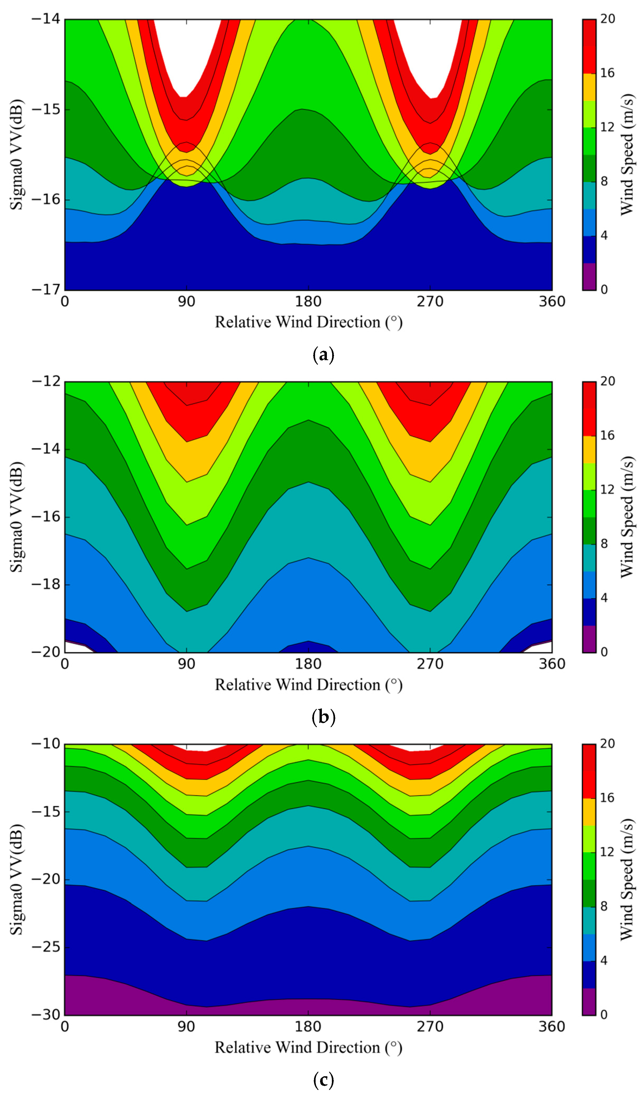
Figure 1 shows the contour plots of SMAP SAR GMF, CMOD5 GMF and NSCAT2 GMF in 40° incidence angles. The contour line of each wind speed is symmetric around the wind direction. At C and Ku band, the maxima of the contour line occur in the upwind (0°) and downwind (180°) directions and minima in the crosswind (90° or 270°) directions. However, the contour lines of low wind speeds overlap ones of moderate and high wind speeds at L band, which is obviously different from C- and Ku-band pattern. This is not explained by the existing directional spreading functions.

3. Methodology

The directional spreading function of the gravity-capillary wave spectrum is related to the radar observation through sea surface backscatter model. We first introduce the directional wave spectrum and propose a basic form of directional spreading function. And then TSM and SPM, which are two basic kinds of sea surface backscatter model, are described and compared. It is generally known that TSM is more suitable for a realistic sea surface due to introduce the double integrals to describe the sea surface tilting effect. However, the double integrals in TSM are very inconvenient to be used to calculate the directional spreading function with radar observations. Fortunately, the solutions of SPM are approximately equal to the TSM solutions in intermediate incidence angles at VV polarization. Finally, we derive the directional spreading function from SPM and calculate its parameters with L-, C- and Ku-band GMFs.

3.1. Basic Form of Directional Spreading Function

The directional wave spectrum can provide the directional distribution of ocean wave energy on the sea surface. With the increase of the quality and quantity of available data, more and more directional wave spectrums have been proposed [22,23]. In most cases the directional wave spectrum $\mathsf{\Psi }\left(k,\varphi \right)$ can be described as a function of both the wave wavenumber and the wave direction relative to the wind as follows:

$$\mathsf{\Psi }\left(k,\varphi \right)=\mathsf{\phi }\left(k\right)·\mathrm{D}\left(k,\varphi \right)$$

(1)

where $k$ is the wave wavenumber, $\varphi$ is the wave direction relative to the wind, $\mathsf{\phi }\left(k\right)$ is the omnidirectional wave spectrum and $\mathrm{D}\left(k,\varphi \right)$ is the directional spreading function defined as:

$$\mathrm{D}\left(k,\varphi \right)=\frac{\mathsf{\Psi }\left(k,\varphi \right)}{{{\displaystyle \int }}_0^{2\pi }\mathsf{\Psi }\left(k,\varphi \right)d\varphi }$$

(2)

If the directional wave spectrum is expressed as a Fourier series, the directional spreading function should contain only even harmonics:

$$\mathrm{D}\left(k,\varphi \right)=\frac{1}{2\pi }[1+{\displaystyle \sum }_{n=1}^{\infty }{\mathrm{a}}_{2n}\cos \left(2n\varphi \right)]$$

(3)

where ${\mathrm{a}}_{2n}$ is the coefficient of even harmonics. In fact the Fourier series expansion is usually truncated to second order [10]:

$$\mathrm{D}\left(k,\varphi \right)=\frac{1}{2\pi }[1+\Delta \left(k\right)\cos \left(2\varphi \right)]$$

(4)

where $\Delta \left(k\right)$ is the second-order harmonic coefficient and the function of both the wavenumber and the wind speed. Unfortunately, up till now the shape of the directional spreading function has been a controversial issue, and the standard form of $\Delta \left(k\right)$ has not been given to correctly unify the gravity and gravity-capillary wave [11]. Here, the form of the directional spreading function from Elfouhaily’s spectrum is used and $\Delta \left(k\right)$ is expressed as:

$$\Delta \left(k\right)=\tanh \{a_0+a_p{\left(c/c_p\right)}^{2.5}+a_m{\left(c_m/c\right)}^{2.5}\}$$

(5)

where $a_0$ and $a_p$ are both constants, $a_m$ is the function of $u^{*}/c_m$, $c$ is the phase speed, $c_p$ is the phase speed of the dominant long wave and $u^{*}$ is the friction velocity at the sea surface. $a_p{\left(c/c_p\right)}^{2.5}$ and $a_m{\left(c_m/c\right)}^{2.5}$ in Equation (5) are related to the directionality of the gravity wave and the gravity-capillary wave, respectively. However, Elfouhaily’s spectrum cannot correctly reflect the directionality of the gravity-capillary wave because radar data is excluded from its development. A correcting term is introduced to replace the gravity-capillary spectral component in the directional spreading function of Elfouhaily’s spectrum:

$$\Delta \left(k\right)=\tanh \{a_p{\left(c/c_p\right)}^{2.5}+\delta \left(k, U_{10}\right)\}$$

(6)

where $a_p$ is equal to 4, $U_{10}$ is the 10-m-height wind speed and $\delta$ is a correction factor which is a function of wavenumber and wind speed.

3.2. Comparison and Selection of Sea Surface Backscatter Model

Sea surface backscatter model can describe the relation between radar observation and directional wave spectrum. The SPM and TSM, which are two basic approaches to calculate ocean-surface scattering, are suitable for the small-scale surface and the tilted small-scale surface, respectively.

3.2.1. Small-Perturbation Method

According to electromagnetic scattering perturbation theory, the Normalized Radar Cross Section (NRCS) of the gravity-capillary wave surface without regard to the tilting effect can be calculated by the first-order SPM [24]:

$${\mathsf{\sigma }}_{0pq}\left(\theta \right)=16\pi k_R^4{\cos }^4\theta {\left|g_{pq}\left(\theta \right)\right|}^2\mathsf{\Psi }\left(2k_R\sin \theta ,\varphi \right)$$

(7)

where ${\mathsf{\sigma }}_0$ is the NRCS, the indices $p$ and $q$ represent transmitting and receiving polarizations, respectively; $k_R$ is the radar wavenumber, $k_R=2\pi /\lambda$, $\lambda$ is the radar wavelength; $\theta$ is the incidence angle; $g_{pq}\left(\theta \right)$ is the first-order scattering coefficient.

3.2.2. Two-Scale Model

In fact, the gravity-capillary waves are tilted by the gravity waves of sea surface. The tilting effect modifies the incidence angle $\theta$ referenced to a horizontal surface as the local angle ${\theta }_i$. Accounting for the sea surface tilting effect, the NRCS is calculated by TSM [24]:

$${\mathsf{\sigma }}_{0pq}\left(\theta \right)={{\displaystyle \int }}_{-\infty }^{\infty }{{\displaystyle \int }}_{-\cot \theta }^{\infty }{\mathsf{\sigma }}_{0pq}\left({\theta }_i\right)P_{\theta }\left(Z_x^{\prime },Z_y^{\prime }\right)d{Z}_{x}d{Z}_y$$

(8)

where $P_{\theta }\left(Z_x^{\prime },Z_y^{\prime }\right)$ is the slope probability density of the gravity wave as viewed at an incidence angle $\theta$. $Z_x$ and $Z_y$ are the slope components for upwind and crosswind, respectively. $Z_x^{\prime }$ and $Z_y^{\prime }$ are expressed as:

$$Z_x^{\prime }=Z_x\cos \varphi +Z_y\sin \varphi$$

(9)

$$Z_y^{\prime }=Z_y\cos \varphi -Z_x\sin \varphi$$

(10)

The relation between the slope probability density function $P_{\theta }\left(Z_x^{\prime },Z_y^{\prime }\right)$ and the function $P\left(Z_x^{\prime },Z_y^{\prime }\right)$ defined by Cox and Munk [25] is:

$$P_{\theta }\left(Z_x^{\prime },Z_y^{\prime }\right)=\left(1+Z_x\tan \theta \right)P\left(Z_x^{\prime },Z_y^{\prime }\right)$$

(11)

The form of $P\left(Z_x^{\prime },Z_y^{\prime }\right)$ is a Gram-Charlier series [25,26]:

$$P\left(Z_x^{\prime },Z_y^{\prime }\right)=\frac{F\left(Z_x^{\prime },Z_y^{\prime }\right)}{2\pi S_u{S}_c}\exp [-\frac{{Z_x^{\prime }}^2}{2{S_u}^2}-\frac{{Z_y^{\prime }}^2}{2{S_c}^2}]$$

(12)

where

$$F\left(Z_x^{\prime },Z_y^{\prime }\right)=1-\frac{C_{21}}{2}\left(\frac{{Z_y^{\prime }}^2}{{S_c}^2}-1\right)\frac{Z_x^{\prime }}{S_u}-\frac{C_{03}}{6}\left(\frac{{Z_x^{\prime }}^2}{{S_u}^3}-\frac{3Z_x^{\prime }}{S_u}\right)+\frac{C_{40}}{24}\left(\frac{{Z_y^{\prime }}^4}{{S_c}^4}-6\frac{{Z_y^{\prime }}^2}{{S_c}^2}+3\right)+\frac{C_{22}}{4}\left(\frac{{Z_y^{\prime }}^2}{{S_c}^2}-1\right)\left(\frac{{Z_x^{\prime }}^2}{{S_u}^2}-1\right)+\frac{C_{04}}{24}\left(\frac{{Z_x^{\prime }}^4}{{S_u}^4}-6\frac{{Z_x^{\prime }}^2}{{S_u}^2}+3\right)$$

(13)

where $C_{40}=0.4$, $C_{22}=0.12$, $C_{04}=0.23$, $C_{21}=0.01-0.0086U$, ${S_u}^2=0.005+0.78\times {10}^{-3}U$, $C_{03}=0.04-0.033U$, ${S_c}^2=0.003+0.84\times {10}^{-3}U$.

TSM is more suitable for a realistic sea surface than SPM because accurately expressing the sea surface tilting effect with the double integrals. But the double integrals bring the difficulty for directly calculating the directional spreading function from TSM. In order to simplify the derivation and calculation of directional spreading function, we find in which case the solutions of SPM are approximately equal to ones of TSM by comparing radar backscatters calculated by SPM and TSM in the following section.

3.2.3. Comparison of SPM and TSM

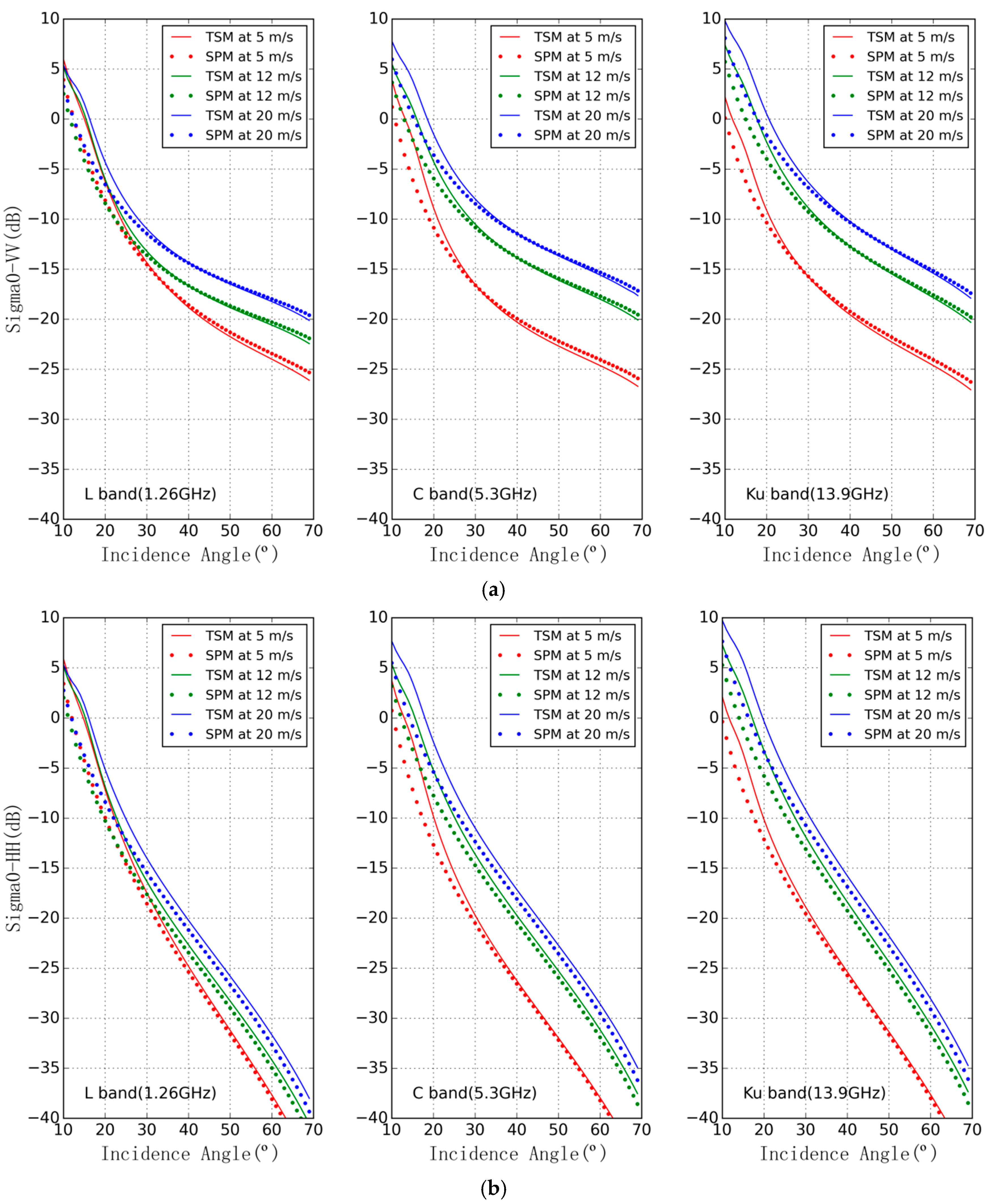
Figure 2 shows VV- and HH-polarization NRCS at 5, 12 and 20 m/s wind speeds, which is calculated by SPM and TSM at L-, C- and Ku-band radar frequencies using Elfouhaily’s omnidirectional spectrum. For HH polarization, there is an evident disagreement of NRCS calculated by SPM and TSM, especially for high wind speed. This is because the gravity-capillary waves are riding on the gravity waves and are thus tilted with respect to the horizontal. For VV polarization, within the range of about 35°–40° incidence angles, there are a very good agreement between the SPM and TSM solutions. It means that the tilting effect from the gravity waves cannot significantly modify the VV-polarization NRCS and the SPM solutions are approximately equal to the TSM solutions within 35°–40° incidence angles.

3.3. Derivation and Calculation of Directional Spreading Function

Wright [27] demonstrated that NRCS calculated by TSM compare favorably with measurements. However, double integrals in TSM (Equation (6)) are very inconvenient to derive the directional spreading function of the gravity-capillary wave spectrum. Fortunately, within 35°–40° incidence angles, the SPM solutions are very close to the TSM solutions at VV polarization. That means the VV-polarization NRCS calculated by Equation (7) is equal to Equation (8). Therefore Equation (7) can be used to retrieve the directional spreading function of the gravity-capillary wave spectrum at VV polarization within 35°–40° incidence angles.

According to Equation (7), the directional spreading function is written as:

$$\mathrm{D}\left(k_B,\varphi \right)=\frac{{\mathsf{\sigma }}_{0vv}{\tan }^4\theta }{\pi k_B^4{\left|g_{vv}\left(\theta \right)\right|}^2\mathsf{\phi }\left(k_B\right)}$$

(14)

where $k_B$ is the wavenumber of the Bragg resonance ocean wave component and related to the radar wavenumber by $k_B=2k_R\sin \theta$, ${\mathsf{\sigma }}_{0vv}$ represents VV-polarization NRCS and is measured by radar. An empirical functional relationship between the VV-polarization NRCS ${\mathsf{\sigma }}_{0vv}$, the 10-m-height wind speed $U_{10}$, the relative wind direction $\varphi$ (the radar azimuth angle with respect to the wind direction) and the incidence angle $\theta$ is generally expressed as:

$${\mathsf{\sigma }}_{0vv}=A_0\left(U_{10},\theta \right)\left(1+A_1\left(U_{10},\theta \right)\cos \varphi +A_2\left(U_{10},\theta \right)\cos 2\varphi \right)$$

(15)

where the $A_1$ term describes the upwind-downwind difference of NRCS. The difference is weak and cannot be attributed to the contribution of ocean wave spectrum [13]. We do not discuss the upwind-downwind difference in this paper. The $A_2$ term describes the upwind-crosswind asymmetry of NRCS and is calculated by:

$$A_2\left(U_{10},\theta \right)=\frac{{\mathsf{\sigma }}_{0vv}^{upwind}+{\mathsf{\sigma }}_{0vv}^{downwind}-2{\mathsf{\sigma }}_{0vv}^{crosswind}}{{\mathsf{\sigma }}_{0vv}^{upwind}+{\mathsf{\sigma }}_{0vv}^{downwind}+2{\mathsf{\sigma }}_{0vv}^{crosswind}}$$

(16)

where ${\mathsf{\sigma }}_{0vv}^{upwind}$, ${\mathsf{\sigma }}_{0vv}^{downwind}$ and ${\mathsf{\sigma }}_{0vv}^{crosswind}$ are the VV-polarization NRCS along the upwind (0°), downwind (180°) and crosswind (90° or 270°) directions, respectively. Because the radar-observed NRCS is proportional to the directional spreading function in Equation (14), the $A_2$ term can be analogous to the second-order harmonic coefficient $\Delta \left(k\right)$ in the directional spreading function of the gravity-capillary wave. Therefore, the second-order harmonic coefficient $\Delta \left(k\right)$ is expressed as:

$$\Delta \left(k\right)=\frac{{\mathsf{\sigma }}_{0vv}^{upwind}+{\mathsf{\sigma }}_{0vv}^{downwind}-2{\mathsf{\sigma }}_{0vv}^{crosswind}}{{\mathsf{\sigma }}_{0vv}^{upwind}+{\mathsf{\sigma }}_{0vv}^{downwind}+2{\mathsf{\sigma }}_{0vv}^{crosswind}}$$

(17)

Presently, the L-, C- and Ku-band GMFs, which empirically relate the NRCS, the 10-m-height wind speed, the relative wind direction and the incidence angle, are better developed than other frequencies with radar observation. The combination of the L, C and Ku bands provide a good coverage of the gravity-capillary wave spectrum for the wavenumber ranging from 25 to 500 rad/m. These GMFs can provide the ${\mathsf{\sigma }}_{0vv}^{upwind}$, ${\mathsf{\sigma }}_{0vv}^{downwind}$ and ${\mathsf{\sigma }}_{0vv}^{crosswind}$ at the three frequency bands and are used to derive a directional spreading function of the gravity-capillary wave.

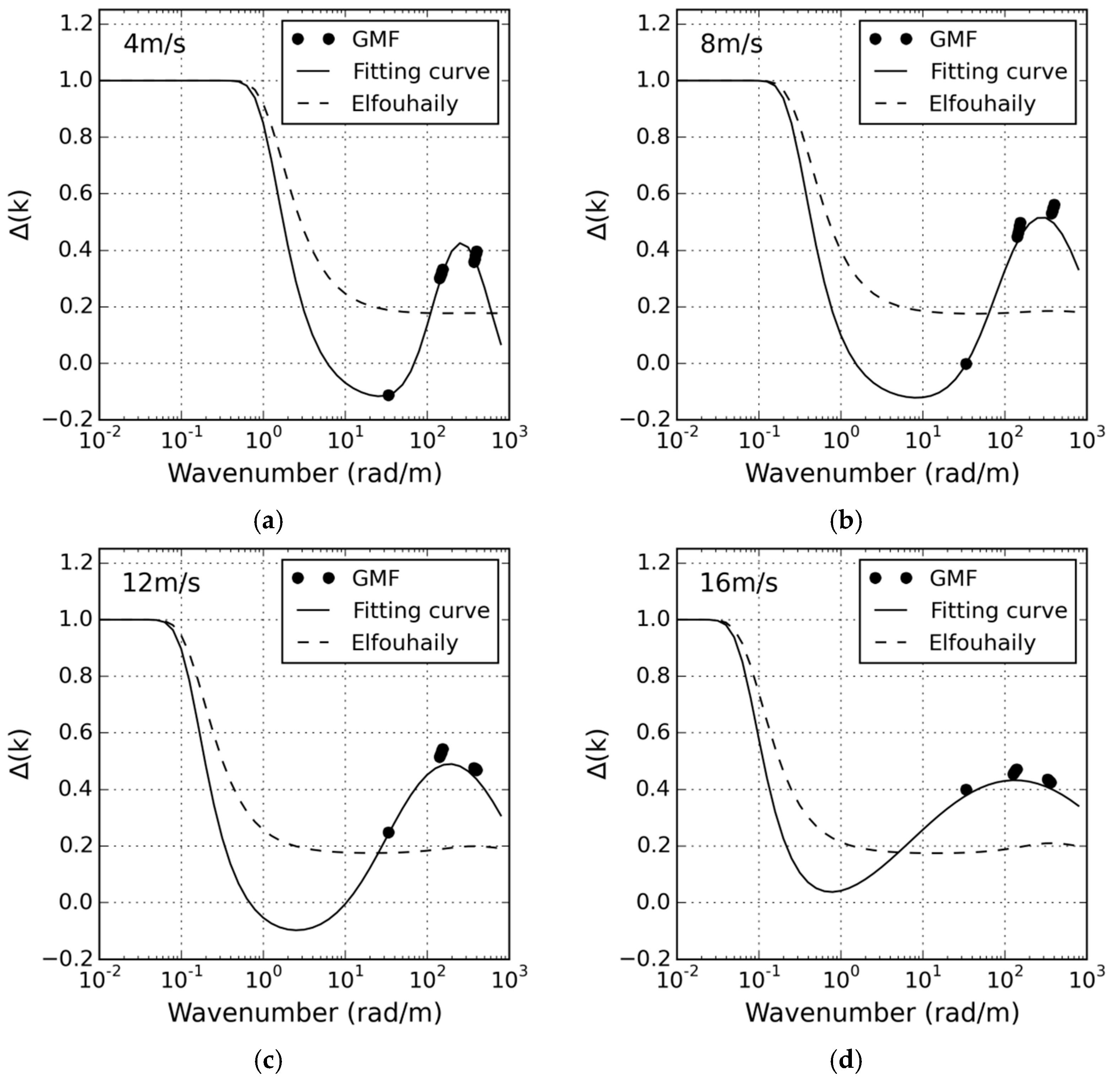
The following calculations are based on the L-band GMF, CMOD5 GMF, and NSCAT2 GMF. Figure 3 shows that the second-order harmonic coefficient $\Delta \left(k\right)$ from L-, C- and Ku-band GMF in 35°–40° incidence angles vary with the wavenumber. The L-band $\Delta \left(k\right)$ is obviously less than the C- and Ku-band ones at all wind speeds, and even is negative at low wind speeds. That indicates that the upwind-crosswind asymmetry of NRCS at L band is weaker than ones at C and Ku band. However, the Elfouhaily’s $\Delta \left(k\right)$ has very little variation in the wavenumber ranging from 10 to 1000 rad/m (contain L, C and Ku band) and is positive at all wind speeds. That cannot explain the obvious variation in L-, C- and Ku-band $\Delta \left(k\right)$ from radar observations, and is inconsistent with the L-band negative value of radar observations at low wind speeds [15]. Therefore a new directional spreading function should be developed to explain these azimuthal behaviors.

According to Equation (17), we use the NRCSs from L-, C- and Ku-band GMF at 35°–40° incidence angle and 2–20 m/s wind speed range to calculate the second-order harmonic coefficient $\Delta \left(k\right)$ at wavenumbers of 30–33, 127–142, 333–374 rad/m. And then the second-order harmonic coefficient $\Delta \left(k\right)$ at the full gravity-capillary wave region is derived by fitting the L-, C- and Ku-band $\Delta \left(k\right)$ to Equation (6) with the Least-Squares-Fitting (LSF) method. $\mathsf{\delta }\left(k,U_{10}\right)$ in Equation (6) is written as:

$$\mathsf{\delta }\left(k,U_{10}\right)={\mathsf{\delta }}_0+{10}^{B_1{K}^2+B_{2}K+B_3}$$

(18)

where ${\delta }_0$ is a constant and equal to −0.1467; $K=lo{g}_{10}\left(k\right)$, $k$ is expressed in radian per meter; $B_1$, $B_2$ and $B_3$ are the regression coefficients and can be derived in each wind-speed bin. The cubic functions of wind speed are used to model $B_1$, $B_2$ and $B_3$ by the LSF method.

$$B_1=p_{13}{U}_{10}^3+p_{12}{U}_{10}^2+p_{11}{U}_{10}+p_{10}$$

(19)

$$B_2=p_{23}{U}_{10}^3+p_{22}{U}_{10}^2+p_{21}{U}_{10}+p_{20}$$

(20)

$$B_3=p_{33}{U}_{10}^3+p_{32}{U}_{10}^2+p_{31}{U}_{10}+p_{30}$$

(21)

where $p_{1i}$, $p_{2i}$ and $p_{3i}$ are the coefficients of the cubic functions and given in

Table 1. The regression coefficients for $B_1$, $B_2$ and $B_3$.

Coefficients	${\mathit{p}}_{\mathit{i}3}$	${\mathit{p}}_{\mathit{i}2}$	${\mathit{p}}_{\mathit{i}1}$	${\mathit{p}}_{\mathit{i}0}$
$B_i\left(i=1\right)$	3.6924 × 10−3	−2.1047 × 10−1	3.9774	−2.5721 × 101
$B_i\left(i=2\right)$	−3.2332 × 10−3	1.8138 × 10−1	−3.3790	2.1479 × 101
$B_i\left(i=3\right)$	7.1639 × 10−4	−3.9639 × 10−2	7.2625 × 10−1	−4.5533

.

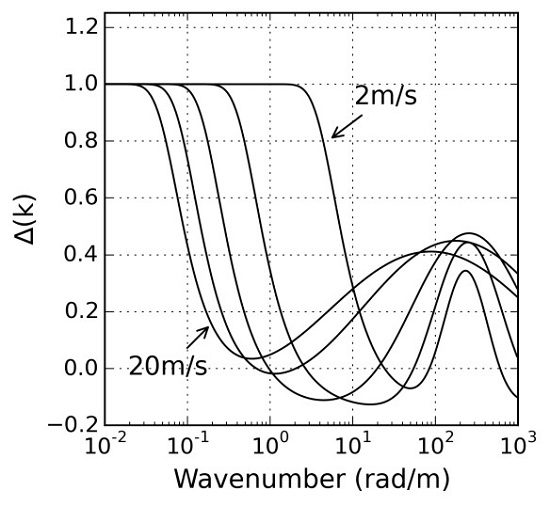
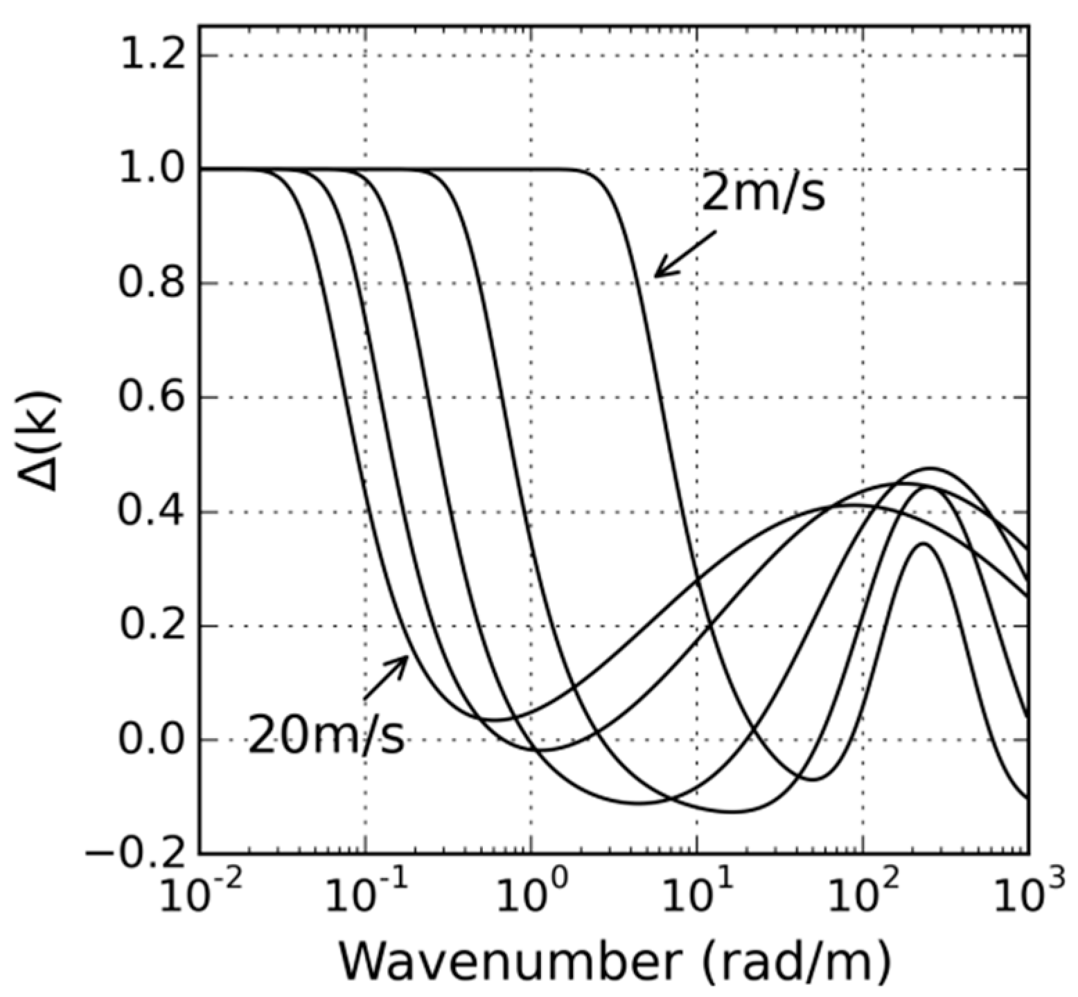
According to Equations (6) and (18)–(21), we plots the proposed second-order harmonic coefficient $\Delta \left(k\right)$ as a function of wavenumber for wind speeds from 2 m/s to 20 m/s with a 4 m/s step in Figure 4. The proposed $\Delta \left(k\right)$ is 1 in the gravity wave region and then decreases with the increasing wavenumber. When the wavenumber is close to the gravity-capillary wave region, the proposed $\Delta \left(k\right)$ drops to the nadir. The nadir is even negative at low and moderate speed range (2–14 m/s). This feature is confirmed by radar observation but is not reflected by the previous models, such as directional spreading functions of Apel [10], Caudal et al. [11] and Elfouhaily et al. [14]. When the wavenumber is in the gravity-capillary wave region, there exists obviously the peak, which will move toward the low wavenumber under the conditions of high wind speeds. The value of peak varies with the wind speed. Its maximum is about 0.4759 and occurs at the wind speed of about 10 m/s and the wavenumber of about 260 rad/m where the gravity-capillary wave spectrum shows the strongest dependence on the direction.

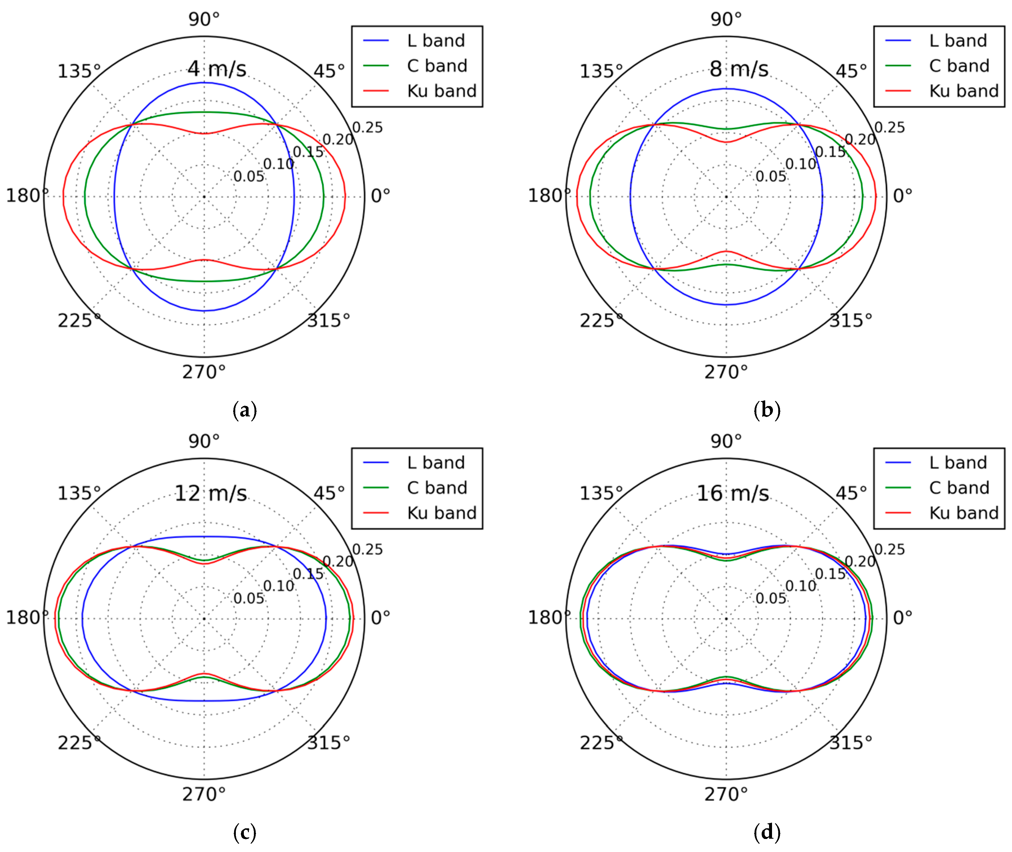
Figure 5 shows the proposed directional spreading function of L, C and Ku band at wind speeds of 4, 8, 12, 16 m/s in polar coordinate. The C- and Ku-band amplitudes at all wind speeds (4, 8, 12 and 16 m/s) and the L-band amplitude at high wind speeds (12 and 16 m/s) along upwind (0°) or downwind (180°) directions are evidently greater than one along crosswind (90° or 270°) directions. In contrast, the L-band amplitude at low and moderate wind speeds (4 and 8 m/s) along upwind (0°) or downwind (180°) directions is less than one along crosswind (90° or 270°) directions, which signifies the negative upwind–crosswind asymmetry. It is consistent with the directional feature observed by Yueh et al. [17], Zhou et al. [18] and Isoguchi et al. [28]. In addition, the difference of the directional spreading function between L, C and Ku band decreases with the increase of wind speed. When the wind speed increases to 16 m/s, the maximum difference is less than 0.02, which means that the directional spreading function of the gravity-capillary wave spectrum has very little variation with the frequency (wavenumber) at high wind speeds.

4. Verification of Directional Spreading Function

The gravity-capillary wave spectrum is not obtained with traditional wave measuring techniques, and therefore it is not feasible to directly verify the proposed directional spreading function of the gravity-capillary wave spectrum with field data at present. Fortunately, the radar backscatter carries the information of the directional wave spectrum due to the Bragg resonance, thus the proposed directional spreading function can be verified by radar observations from the L-band SAR on the SMAP satellite, the C-band ASCAT scatterometer on the METOP-A satellite and the Ku-band SeaWinds-1 scatterometer on the QuikSCAT satellite. SMAP SAR NRCS, simultaneous DMSP F17 SSMI/S wind speed and NCEP wind direction are used to act as the L-band validation data, and its time range is from 18 to 28 April 2015. ASCAT NRCS and wind field are used to act as the C-band validation data, and its time range from 1 to 10 February 2010. SeaWinds-1 NRCS and wind field are used to act as the Ku-band validation data, and its time range is from 1 to 10 January 2008.

According to Equation (4), the accuracy of the directional spreading function is closely related to the second-order harmonic coefficient $\Delta \left(k\right)$, which can be calculated by the VV-polarization NRCS from radar observation along the upwind, downwind and crosswind directions. Therefore, we validate the accuracy of the directional spreading function by comparing the proposed second-order harmonic coefficients and the radar-observed second-order harmonic coefficients.

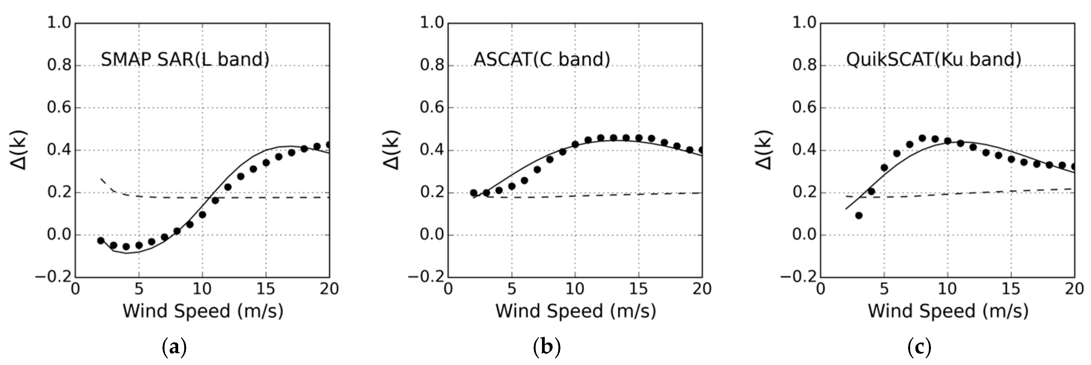
Figure 6 shows the comparisons of the second-order harmonic coefficient $\Delta \left(k\right)$ from the proposed direction spreading function, radar observation and Elfouhaily’s spectrum at L, C and Ku band at 2–20 m/s wind speed range. The incidence angles of L-band data from SMAP SAR and C-band data from ASCAT are both 40°, and one of Ku-band data from SeaWinds-1 is 55°. The proposed $\Delta \left(k\right)$ varies with wind speeds and is basically consistent with one from radar observation. Other than the above two ones, the Elfouhaily’s $\Delta \left(k\right)$, which is about 0.2 and has very little variation with wind speeds especially at C and Ku band, is inconsistent with radar observation. The comparisons between the three second-order harmonic coefficients indicates that the proposed direction spreading function is more consistent with radar observation than Elfouhaily’s spectrum, which is also reflected by the statistics of the comparisons in

Table 2. Statistics of the proposed $\Delta \left(k\right)$ and Elfouhaily’s $\Delta \left(k\right)$ versus the radar-observed $\Delta \left(k\right)$ at 2–20 m/s wind speed range.

$\Delta \left(\mathit{k}\right)$	L Band		C Band		Ku Band
	RMSD	CC	RMSD	CC	RMSD	CC
the proposed $\Delta \left(k\right)$	0.0438	0.9745	0.0263	0.9656	0.0382	0.9009
Elfouhaily’s $\Delta \left(k\right)$	0.2005	−0.3965	0.0909	0.5840	0.0887	−0.0257

.

Table 2 shows the RMSD and CC of the proposed $\Delta \left(k\right)$ and Elfouhaily’s $\Delta \left(k\right)$ versus the radar-observed $\Delta \left(k\right)$ at L, C and Ku band at 2–20 m/s wind speed range. The radar-observed $\Delta \left(k\right)$ acts as sea truth data. The L-band RMSD and CC of the proposed $\Delta \left(k\right)$ is 0.0438 and 0.9745, respectively. The C- and Ku-band RMSDs are reduced to 0.0263 and 0.0382, respectively, and their CCs are reduced to 0.9656 and 0.9009, respectively. Overall, the proposed $\Delta \left(k\right)$ has the high accuracy and is remarkably consistent with radar observation. In addition, it is obvious that the RMSD of Elfouhaily’s $\Delta \left(k\right)$ is greater than one of the proposed $\Delta \left(k\right)$, and its CC is less than one of the proposed $\Delta \left(k\right)$. In other words, the accuracy of the proposed $\Delta \left(k\right)$ is much higher than Elfouhaily’s $\Delta \left(k\right)$ because the development of Elfouhaily’s spectrum does not introduce radar data, which contain the information of the gravity-capillary waves.

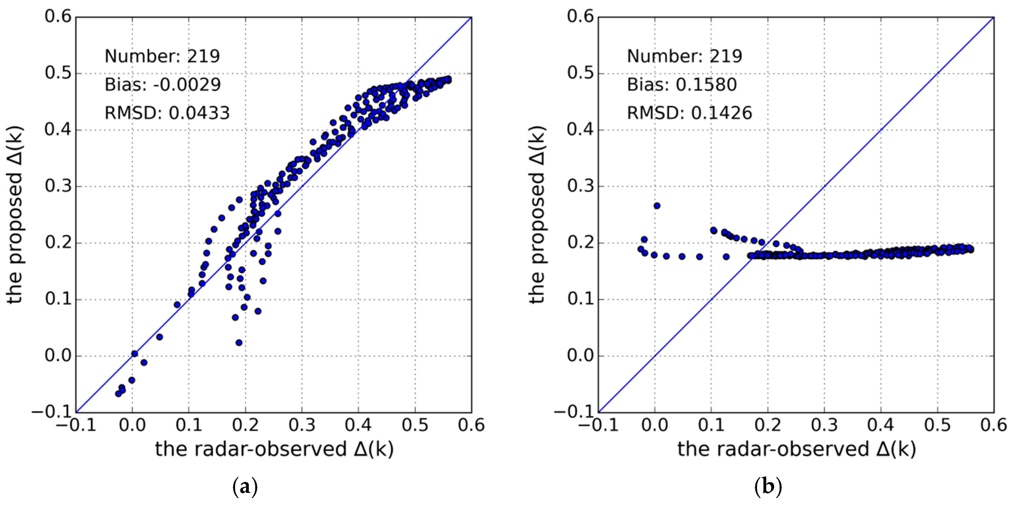
Figure 7 shows the scatterplots of the proposed $\Delta \left(k\right)$ and Elfouhaily’s $\Delta \left(k\right)$ versus the radar-observed $\Delta \left(k\right)$ at L, C and Ku band at 2–20 m/s wind speed range. The incidence angles of L-band data from SMAP SAR and Ku-band data from SeaWinds-1 is 40° and 55°, respectively, and ones of C-band data from ASCAT is from 35° to 45°. The radar-observed $\Delta \left(k\right)$ acts as sea truth data. Figure 7a shows that the proposed $\Delta \left(k\right)$ is basically consistent with radar observation. The bias and RMSD of the proposed versus the radar-observed $\Delta \left(k\right)$ are −0.0029 and 0.0433, respectively. Figure 7b shows that Elfouhaily’s $\Delta \left(k\right)$ is a serious deviation from radar observation and its bias and RMSD are 0.1580 and 0.1426, respectively. Obviously, the proposed $\Delta \left(k\right)$ is more consistent with radar observation than Elfouhaily’s $\Delta \left(k\right)$.

In conclusion, the proposed direction spreading function has the high accuracy and is basically consistent with radar observation on the basis of comparisons and statistics of the second-order harmonic coefficient.

5. Discussion

At present, there is no standard form of the directional spreading function to correctly unify the gravity and gravity-capillary wave. If the directional wave spectrum is expressed as a Fourier series, the cosine-shape spreading function proposed by Longuet-Higgines et al. [3], Mitsuyasu et al. [4], Hasselmann et al. [5], and the sech-shape spreading function proposed by Donelan et al. [6] are all transformed into the hyperbolic tangent form. Due to the natural involvement of the hyperbolic tangent function, the proposed directional spreading function in this paper, which introduces a correcting term to replace the gravity-capillary spectral component in the directional spreading function of Elfouhaily’s spectrum, is a good choice to unify the gravity and gravity-capillary wave. The correcting term is a function of wavenumber and wind speed with twelve adjusted parameters, which are derived from L-, C- and Ku-band radar backscatter. It is noted that the X-band GMF has been developed by Li et al. [29] and Ren et al. [30]. But the upwind-crosswind asymmetry in their GMFs needs to be verified by large amounts of data. Therefore, the better developed L-, C- and Ku-band GMFs are only used to derive and verify the directional spreading function of the gravity-capillary wave spectrum.

6. Conclusions

In this paper, the directional spreading function of the gravity-capillary wave spectrum is expressed as the second-order Fourier series expansion. It is worthwhile to note that no standard form of the second-order harmonic coefficient has been given to correctly unify the gravity and gravity-capillary wave at the present. Our strategy is to introduce a correcting term to replace the inaccurate gravity-capillary spectral component in Elfouhaily’s directional spreading function. And then we derive the correcting term from radar observations.

The Two-Scale Model (TSM) is widely applied to describe the relation between radar observation and directional wave spectrum, but has double integrals to be very inconvenient to study the directional spectrum. Fortunately, the comparison of radar backscatters calculated by Small-Perturbation Method (SPM) and TSM shows that the SPM solutions are approximately equal to the TSM solutions for VV polarization within 35°–40° incidence angles. So we use the SPM to relate radar observations at VV polarization within intermediate incidence angles to the directional wave spectrum.

The radar-observed Normalized Radar Cross Section (NRCS) is proportional to the directional spreading function in radar backscatter model of SPM. So the upwind-crosswind asymmetry of NRCS is analogous to the second-order harmonic coefficient in the directional spreading function. The second-order harmonic coefficient at wavenumbers of 30–33, 127–142, 333–374 rad/m calculated by the NRCS is used to fit the correcting term to obtain one at the full gravity-capillary wave region by the Least-Squares-Fitting (LSF) method. According to the proposed second-order harmonic coefficient, we find that there is the obvious peak at the gravity-capillary wave region, which varies with the wind speed. In addition, there exist the negative values at low and moderate wind speeds in proposed second-order harmonic coefficient, which is different from the previous model but has been confirmed by the L-band radar observation. The Root Mean Square Difference (RMSD) of the proposed second-order harmonic coefficient versus the L-, C- and Ku-band radar-observed one from SMAP SAR, ASCAT and SeaWinds-1 are 0.0438, 0.0263 and 0.0382, respectively. The L-, C- and Ku-band Correlation Coefficient (CC) is 0.9745, 0.9656 and 0.9009, respectively. The overall bias and RMSD are −0.0029 and 0.0433 for the whole second-order harmonic coefficient range, respectively. This means that the proposed second-order harmonic coefficient in the paper has the high accuracy and is consistent with radar observation at L, C and Ku band.

This paper verifies the proposed second-order harmonic coefficient with L-, C- and Ku-band NRCS. It is worthwhile to note that the proposed second-order harmonic coefficient is derived at the full gravity-capillary wave region and the accuracy at other microwave frequency bands needs to be quantitatively verified. With the increase of the quality and quantity of available data at other microwave frequency bands, the future work will be able to further verify and improve it.

References

- Sullivan, P.P.; McWilliams, J.C. Dynamics of winds and currents coupled to surface waves. Annu. Rev. Fluid Mech. 2010, 42, 19–42. [Google Scholar] [CrossRef]
- Long, S. Wind-generated water waves in a wind tunnel: Free surface statistics, wind friction and mean air flow properties. Coast. Eng. 2012, 61, 27–41. [Google Scholar] [CrossRef]
- Longuet-Higgins, M.S.; Cartwright, D.E.; Smith, N.D. Observations of the directional spectrum of sea waves using the motions of a floating buoy. In Ocean Wave Spectra; Prentice-Hall: Upper Saddle River, NJ, USA, 1963; pp. 111–136. [Google Scholar]
- Mitsuyasu, H.; Tasai, F.; Suhara, T.; Mizuno, S.; Ohkusu, M.; Honda, T.; Rikiishi, K. Observation of the directional wave spectra of ocean waves using a cloverleaf buoy. J. Phys. Oceanogr. 1975, 5, 750–760. [Google Scholar] [CrossRef]
- Hasselmann, D.E.; Dunckel, M.; Ewing, J.A. Directional wave spectra observed during JONSWAP 1973. J. Phys. Oceanogr. 1980, 10, 1264–1280. [Google Scholar] [CrossRef]
- Donelan, M.A.; Hamilton, J.; Hui, W.H. Directional spectra of wind-generated waves. Philos. Trans. R. Soc. Lond. 1985, 315, 509–562. [Google Scholar] [CrossRef]
- Shao, W.; Zhang, Z.; Li, X.; Li, H. Ocean wave parameters retrieval from Sentinel-1 SAR imagery. Remote Sens. 2016, 8. [Google Scholar] [CrossRef]
- Shao, W.; Li, X.; Sun, J. Ocean Wave Parameters Retrieval from TerraSAR-X Images Validated against Buoy Measurements and Model Results. Remote Sens. 2015, 7, 12815–12828. [Google Scholar] [CrossRef]
- Li, X.; Pichel, W.; He, M.; Wu, S.; Friedman, K.; Clemente-Colon, P.; Zhao, C. Observation of Hurricane-Generated Ocean Swell Refraction at the Gulf Stream North Wall with the RADARSAT-1 Synthetic Aperture Radar. IEEE Trans. Geosci. Remote Sens. 2002, 40, 2131–2142. [Google Scholar]
- Apel, J.R. An improved model of the ocean surface wave vector spectrum and its effects on radar backscatter. J. Geophys. Res. 1994, 99, 16269–16291. [Google Scholar] [CrossRef]
- Caudal, G.; Hauser, D. Directional spreading function of the sea wave spectrum at short scale, inferred from multifrequency radar observations. J. Geophys. Res. 1996, 101, 16601–16613. [Google Scholar] [CrossRef]
- Liu, Y.G.; Yan, X.H. The wind-induced wave growth rate and the spectrum of the gravity-capillary waves. J. Phys. Oceanogr. 1995, 25, 3196–3218. [Google Scholar] [CrossRef]
- Gutssard, A. Directional spectrum of the sea surface and wind scatterometry. Int. J. Remote Sens. 1993, 14, 1615–1633. [Google Scholar] [CrossRef]
- Elfouhaily, T.; Chapron, B.; Katsaros, K.; Vandemark, D. A unified directional spectrum for long and short wind-driven waves. J. Geophys. Res. 1997, 102, 15781–15796. [Google Scholar] [CrossRef]
- Hwang, P.; Wang, D.W.; Walsh, E.J.; Krabill, W.B.; Swift, R.N. Airborne measurements of the wavenumber spectra of ocean surface waves. Part II: Directional distribution. J. Phys. Oceanogr. 2010, 30, 2768–2787. [Google Scholar] [CrossRef]
- Yueh, S.H.; Tang, W.A.; Fore, G.; Neumann, G.; Hayashi, A.; Freedman, A.; Chaubell, J.; Lagerloef, G.S.E. L-band passive and active microwave geophysical model functions of ocean surface winds and applications to aquarius retrieval. IEEE Trans. Geosci. Remote Sens. 2013, 51, 4619–4632. [Google Scholar] [CrossRef]
- Yueh, S.H.; Tang, W.A.; Fore, G.; Hayashi, A.K.; Song, Y.T.; Lagerloef, G. Aquarius geophysical model function and combined active passive algorithm for ocean surface salinity and wind retrieval. J. Geophys. Res. Oceans 2014, 119, 5360–5379. [Google Scholar] [CrossRef]
- Zhou, X.; Chong, J.S.; Yang, X.F.; Li, W.; Guo, X.X. Ocean Surface Wind Retrieval using SMAP L-Band SAR. IEEE J. Sel. Top. Appl. Earth Obs. Remote Sens. 2017, 10, 65–74. [Google Scholar] [CrossRef]
- Hersbach, H.; Stoffelen, A.; de Haan, S. An improved C-band scatterometer ocean geophysical model function: CMOD5. J. Geophys. Res. 2007, 112. [Google Scholar] [CrossRef]
- Wentz, F.J.; Smith, D.K. A model function for the ocean-normalized radar cross section at 14 GHz derived from NSCAT observations. J. Geophys. Res. 1999, 104, 11499–11514. [Google Scholar] [CrossRef]
- Hwang, P. Ocean Surface Roughness Spectrum in High Wind Condition for Microwave Backscatter and Emission Computations. J. Atmos. Ocean. Technol. 2013, 30, 2168–2188. [Google Scholar] [CrossRef]
- Yurovskaya, M.V.; Dulov, V.A.; Chapron, B.; Kudryavtsev, V.N. Directional short wind wave spectra derived from the sea surface photography. J. Geophys. Res. Oceans 2013, 118, 4380–4394. [Google Scholar] [CrossRef]
- Hwang, P. A note on the ocean surface roughness spectrum. J. Atmos. Ocean. Technol. 2011, 28, 436–443. [Google Scholar] [CrossRef]
- Valenzuela, G.R. Theories for the interaction of electromagnetic and oceanic waves—A review. Bound. Layer Meteorol. 1978, 13, 61–85. [Google Scholar] [CrossRef]
- Cox, C.; Munk, W. Measurement of the roughness of the sea surface from photographs of the sun glitter. J. Opt. Soc. Am. 1954, 44, 838–850. [Google Scholar] [CrossRef]
- Fung, A.K.; Lee, K.K. A Semi-Empirical Sea-Spectrum Model for Scattering Coefficient Estimation. IEEE J. Ocean. Eng. 1982, 7, 166–176. [Google Scholar] [CrossRef]
- Wright, J.W. A new model for sea clutter. IEEE Trans. Antennas Propag. 1968, 16, 217–223. [Google Scholar] [CrossRef]
- Isoguchi, O.; Shimada, M. An L-band ocean geophysical model function derived from PALSAR. IEEE Trans. Geosci. Remote Sens. 2009, 47, 1925–1936. [Google Scholar] [CrossRef]
- Li, X.M.; Lehner, S. Algorithm for Sea Surface Wind Retrieval from TerraSAR-X and TanDEM-X Data. IEEE Trans. Geosci. Remote Sens. 2014, 52, 2928–2939. [Google Scholar] [CrossRef]
- Ren, Y.Z.; Li, X.M.; Zhou, G.Q. Sea Surface Wind Retrievals from SIR-C/X-SAR Data: A Revisit. Remote Sens. 2015, 7, 3548–3564. [Google Scholar] [CrossRef]
Figure 1.
The SMAP SAR GMF (a); CMOD5 GMF (b) and NSCAT2 GMF (c) in 40° incidence angles.
Figure 2.
Comparison of VV- (a) and HH- (b) polarization NRCS calculated by SPM and TSM at L band (1.26 GHz), C band (5.3 GHz) and Ku band (13.9 GHz).
Figure 3.
The second-order harmonic coefficient inferred from the GMFs in 35°–40° incidence angles, Elfouhaily’s spectrum and fitting curves plots as a function of wavenumber at wind speeds of 4 (a); 8 (b); 12 (c); 16 (d) m/s.
Figure 4.
The proposed second-order harmonic coefficient plots as a function of wavenumber for wind speeds from 2 m/s to 20 m/s with a 4 m/s step.
Figure 5.
The L-, C- and Ku-band directional spreading function plots as a function of the wave direction relative to the wind at wind speeds of 4 (a); 8 (b); 12 (c); 16 (d) m/s.
Figure 6.
Comparisons of the from the proposed direction spreading function(solid lines), radar observations (dotted lines) and Elfouhaily’s spectrum (dashed lines) at L (a), C (b) and Ku (c) band at 2–20 m/s wind speed range.
Figure 7.
The radar-observed versus the proposed (a) and Elfouhaily’s (b).