
Evaluation of Remote Sensing Inversion Error for the Above-Ground Biomass of Alpine Meadow Grassland Based on Multi-Source Satellite Data

 ,
,  and
and
Abstract
:
1. Introduction
2. Data and Methods
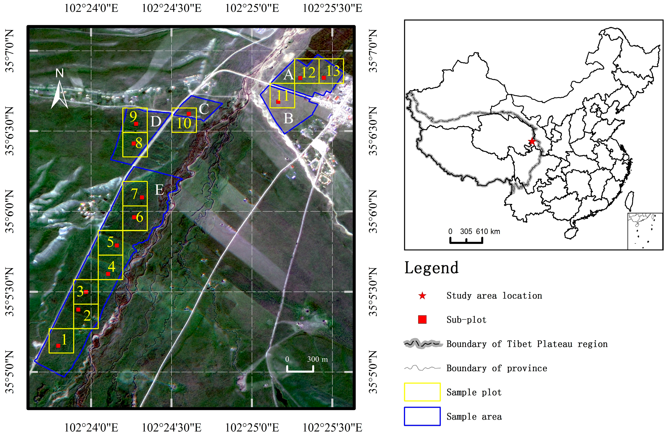
2.1. Study
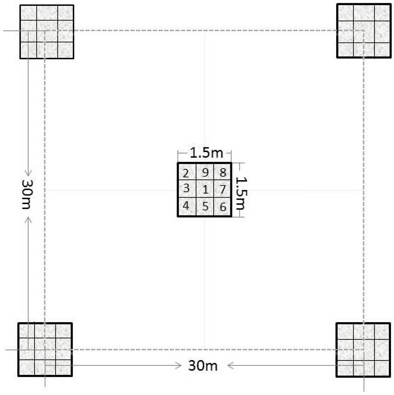
2.2. Sampling Strategy and Data Collection
2.3. Preprocessing of MODIS Vegetation Index Data
2.4. Data Processing of Landsat 8 OLI and HJ-1B CCD and Calculation of the Vegetation Index
2.5. Spectral Data Processing and Accuracy Evaluation of MODIS NDVI
2.6. Construction of Grassland Biomass Monitoring Model and Accuracy Evaluation
3. Results and Analysis
3.1. Statistical Analysis of Ground Observation AGB and the Corresponding Multi-Source Satellite NDVI
3.2. Influence of Different Filtering Methods on MODIS NDVI
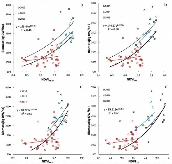
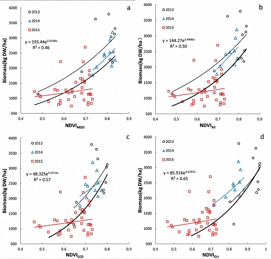
3.3. Grassland Biomass Monitoring Model in the Study Area and Evaluation of Its Accuracy at the Sample Plot Level
4. Discussion
4.1. Influence of Different Remote Sensing Data on the Estimation Error of Grassland Biomass
4.2. Influence of Three Filtering Methods on the Error of Grassland AGB Estimation Based on MODIS NDVI
4.3. Assessment of Previously-Established Biomass Inversion Models Based on the MODIS Vegetation Index over the Tibetan Plateau
4.4. Limitations and Prospects of Remote Sensing Monitoring Biomass
5. Conclusions
- (1)
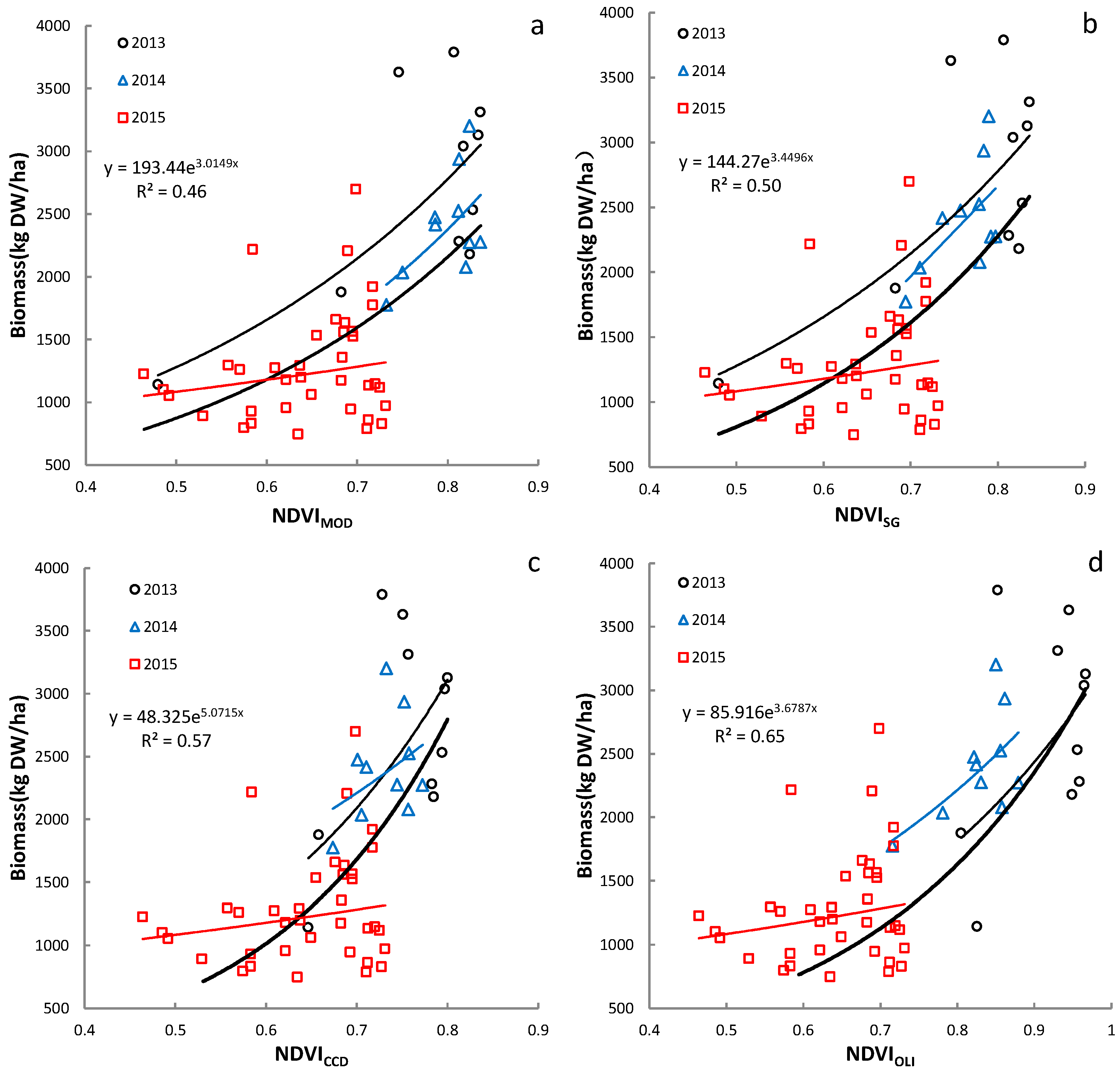
- There is a significant difference in the estimation errors of alpine meadow grassland AGB using remote sensing data from the Chinese HJ-1B CCD, Terra MODIS and Landsat 8 OLI. In this study, the grassland AGB optimum inversion model of the experimental area is the exponential model based on NDVIMOD, NDVIOLI and NDVICCD, but different models show considerable differences in the error of grassland AGB inversion. The errors for the estimation of grassland AGB for the optimum models based on NDVIMOD, NDVICCD and NDVIOLI at the sample plot level are 35.3%, 31.6% and 29.1%, respectively. Their yield per unit area estimations for grassland AGB in the experimental area indicate that the exponential model based on NDVIOLI yielded values closest to the ground-measured value; its estimation error for yield per unit area is the smallest (30.7%). The estimation error for yield per unit area for the experimental area with the optimum AGB inversion model based on NDVIOLI decrease by eight and two percentage points, respectively, compared to the optimum inversion models based on NDVIMOD and NDVICCD.
- (2)
- The filtering and de-noising processing of MOD13Q1 NDVI are key for reducing the AGB inversion error of alpine meadow grassland based on MODIS data. At the sample plot level, the estimation errors of the AGB estimation models based on NDVISG, NDVILO and NDVIGA decreased by 1.40, 1.14 and 1.13 percentage points, respectively, compared to the AGB estimation model based on NDVIMOD. On the study area scale (161.36 ha), the estimation errors for the yield per unit area of grassland AGB based on NDVISG, NDVILO and NDVIGA decreased by 4.48, 0.95 and 0.22, respectively, compared to that based on NDVIMOD.
- (3)
- The feasibility study on previous models (I and II, III and IV and V) developed (on MODIS indices) at broad scales to apply to our small study area suggests that the estimation error of these models is higher than that of the NDVIMOD model constructed in this study by 11.9%–36.4% at the sample plot scale and 5.3%–29.6% at the study area scale. Models V, IV and III based on Xiahe County and Gannan Prefecture do not show considerable difference on the estimation error of AGB, ranging from 47.2%–47.8% at the sample plot level and 44.6%–48.0% of the yield per unit area at the study area level. However, Models I and II based on the Tibetan Plateau scale show much larger estimation error, up to 71.7% and 58.6%, respectively, at the sample plot scale and 68.9% and 48.3% of the yield per unit area at the study area scale.
Acknowledgments
Author Contributions
Conflicts of Interest
References
- Adams, J.M.; Faure, H.; Faure-Denard, L.; McGlade, J.M.; Woodward, F.L. Increases in terrestrial carbon storage from the last glacial maximum to the present. Nature 1990, 348, 711–714. [Google Scholar] [CrossRef]
- White, R.; Murray, S.; Rohweder, M. Pilote Analysis of Global Ecosystems: Grassland Ecosystems; World Resources Institute: Washington, DC, USA, November 2000; Available online: http://earthtrends.wri.org/text/ forests-grasslands-drylands /map-229.htm.
- Scurlock, J.M.O.; Hall, D.O. The global carbon sink: A grassland perspective. Glob. Chang. Biol. 1998, 4, 229–233. [Google Scholar] [CrossRef]
- Feng, X.M.; Zhao, Y.S. Grazing intensity monitoring in Northern China steppe: Integrating CENTURY model and MODIS data. Ecol. Indic. 2011, 11, 175–182. [Google Scholar] [CrossRef]
- Ma, W.H.; Fang, J.Y.; Yang, Y.H.; Mohammat, A. Biomass carbon stocks and their changes in northern China’s grasslands during 1982–2006. Sci. China Life Sci. 2010, 53, 841–850. [Google Scholar] [CrossRef] [PubMed]
- Lauenroth, W.K.; Hunt, H.W.; Swift, D.M.; Singh, J.S. Estimating aboveground net primary production in grasslands—A simulation approach. Ecol. Model. 1986, 33, 297–314. [Google Scholar] [CrossRef]
- Jobbagy, E.G.; Sala, O.E. Controls of Grass and Shrub Aboveground Production in the Patagonian Steppe. Ecol. Appl. 2000, 10, 541–549. [Google Scholar] [CrossRef]
- Soussana, J.F.; Loieau, P.; Vjichard, N.; Ceachia, E.; Balesdent, J.; Chevallier, T.; Arrouays, D. Carbon Cycling and Sequestration Opportunities in Temperate Grasslands. Soil Use Manag. 2004, 20, 219–230. [Google Scholar] [CrossRef]
- Hopkins, A. Relevance and functionality of semi-natural grassland in Europe–status quo and future prospective. In Proceedings of the International Workshop of the Salvere, Raumberg-Gumpenstein, Austria, 26–27 May 2009; pp. 9–14. [Google Scholar]
- Moreau, S.; Bosseno, R.; Gu, X.F.; Baret, F. Assessing the biomass dynamics of Andean bofedal and totora highprotein wetland grasses from NOAA/AVHRR. Remote Sens. Environ. 2003, 85, 516–529. [Google Scholar] [CrossRef]
- Nordberg, M.L.; Evertson, J. Vegetation index differencing and linear regression for change detection in a Swedish mountain range using Landsat TM and ETMt imagery. Land Degrad. Dev. 2004, 16, 139–149. [Google Scholar] [CrossRef]
- Ali, I.; Cawkwell, F.; Dwyer, E.; Barrett, B.; Green, S. Satellite remote sensing of grasslands: From observation to management—A review. J. Plant Ecol. 2016, 9, 649–671. [Google Scholar] [CrossRef]
- Rouse, J.W.; Haas, R.H.; Schell, J.A.; Deering, D.W. Monitoring vegetation systems in the Great Plains with ERTS. In Proceedings of the Third ERTS-1 Symposium, Washington DC, USA, 10–14 December 1973; Fraden, S.C., Marcanti, E.P., Becker, M.A., Eds.; NASA SP-351: Washington, DC, USA, 1973; pp. 309–317. [Google Scholar]
- Tucker, C.J. Red and Photographic Infrared Linear Combinations for Monitoring Vegetation. Remote Sens. Environ. 1979, 8, 127–150. [Google Scholar] [CrossRef]
- Tucker, C.J.; Justice, C.O.; Prince, S.D. Monitoring the grasslands of the Sahel 1984–1985. Int. J. Remote Sens. 1986, 7, 1571–1581. [Google Scholar] [CrossRef]
- Ullah, S.; Si, Y.; Schlerf, M.; Skidmore, A.K.; Shafique, M.; Iqbal, I.A. Estimation of grassland biomass and nitrogen using MERIS data. Int. J. Appl. Earth Obs. Geoinf. 2012, 1, 196–204. [Google Scholar] [CrossRef]
- Li, F.; Zeng, Y.; Li, X.S.; Zhao, Q.J.; Wu, B.F. Remote sensing based monitoring of interannual variations in vegetation activity in China from 1982 to 2009. Sci. China Earth Sci. 2014, 57, 1800–1806. [Google Scholar] [CrossRef]
- Yang, F.; Sun, J.L.; Fang, H.L.; Yao, Z.F.; Zhang, J.H.; Zhu, Y.Q.; Song, K.S.; Wang, Z.M.; Hu, M.G. Comparison of different methods for corn LAI estimation over northeastern China. Int. J. Appl. Earth Obs. Geoinf. 2012, 18, 462–471. [Google Scholar]
- Xu, B.; Yang, X.; Tao, W.; Qin, Z.H.; Liu, H.Q.; Miao, J.M. Remote sensing monitoring upon the grass production in China. Acta Ecol. Sin. 2007, 27, 405–413. [Google Scholar] [CrossRef]
- Li, F.; Zeng, Y.; Luo, J.H.; Ma, R.H.; Wu, B.F. Modeling grassland aboveground biomass using a pure vegetation index. Ecol. Indic. 2016, 62, 279–288. [Google Scholar] [CrossRef]
- Yang, Y.H.; Fang, J.Y.; Pan, Y.D.; Ji, C.J. Aboveground biomass in Tibetan grasslands. J. Arid Environ. 2009, 73, 91–95. [Google Scholar] [CrossRef]
- Xie, Y.; Sha, Z.Y.; Yu, M.; Bai, Y.F.; Zhang, L. A comparison of two models with Landsat data for estimating above ground grassland biomass in Inner Mongolia, China. Ecol. Model. 2009, 220, 1810–1818. [Google Scholar] [CrossRef]
- Chen, J.; Jönsson, P.; Tamura, M.; Gu, Z.H.; Matsushita, B.; Eklundh, L. A simple method for reconstructing a high-quality NDVI time-series data set based on the Savitzky–Golay filter. Remote Sens. Environ. 2004, 91, 332–344. [Google Scholar] [CrossRef]
- Dusseux, P.; Hubert-Moy, L.; Corpetti, T.; Vertès, F. Evaluation of SPOT imagery for the estimation of grassland biomass. Int. J. Appl. Earth Obs. Geoinf. 2015, 38, 72–77. [Google Scholar] [CrossRef]
- Wang, X.P.; Guo, N.; Zhang, K.; Wang, J. Hyperspectral Remote Sensing Estimation Models of Aboveground Biomass in Gannan Rangelands. Procedia Environ. Sci. 2011, 10, 697–702. [Google Scholar]
- Liu, B.K.; Du, Y.E.; Liang, T.G.; Feng, Q.S. Outburst Flooding of the Moraine-Dammed Zhuonai Lake on Tibetan Plateau: Causes and Impacts. IEEE Geosci. Remote Sens. Lett. 2016, 13, 570–574. [Google Scholar] [CrossRef]
- Jia, W.X.; Liu, M.; Yang, Y.H.; He, H.L.; Zhu, X.D.; Yang, F.; Yin, C.; Xiang, W.N. Estimation and uncertainty analyses of grassland biomass in Northern China: Comparison of multiple remote sensing data sources and modeling approaches. Ecol. Indic. 2016, 60, 1031–1040. [Google Scholar] [CrossRef]
- Irons, J.R.; Dwyer, J.L.; Barsi, J.A. The next Landsat satellite: The Landsat Data Continuity Mission. Remote Sens. Environ. 2012, 122, 11–21. [Google Scholar] [CrossRef]
- Geng, L.L.; Ma, M.G.; Wang, X.F.; Yu, W.P.; Jia, S.Z.; Wang, H.B. Comparison of Eight Techniques for Reconstructing Multi-Satellite Sensor Time-Series NDVI Data Sets in the Heihe River Basin, China. Remote Sens. 2014, 6, 2024–2049. [Google Scholar] [CrossRef]
- Feng, Q.S.; Gao, X.H.; Huang, X.D.; Yu, H.; Liang, T.G. Remote sensing dynamic monitoring of grass growth in Qinghai-Tibet plateau from 2001 to 2010. J. Lanzhou Univ. 2011, 47, 75–90. [Google Scholar]
- Cui, X.; Guo, Z.G.; Liang, T.G.; Shen, Y.Y.; Liu, X.Y.; Liu, Y. Classification management for grassland using MODIS data: A case study in the Gannan region, China. Int. J. Remote Sens. 2012, 33, 3156–3175. [Google Scholar] [CrossRef]
- Wang, Y.; Xia, W.T.; Liang, T.G.; Wang, C. Spatial and temporal dynamic changes of net primary product based on MODIS vegetation index in Gannan grassland. Acta Pratacult. Sin. 2010, 19, 201–210. [Google Scholar]
- Bao, H.M. Dynamic Monitoring and Prediction of Aboveground Biomass of Natural Grassland—A Case Study in Xiahe County of Gansu Province. Master’s Thesis, Gansu Agricultural University, Lanzhou, China, 2010. [Google Scholar]
- Porter, T.F.; Chen, C.C.; Long, J.A.; Lawrence, R.L.; Sowell, B.F. Estimating biomass on CRP pastureland: A comparison of remote sensing techniques. Biomass Energy 2014, 66, 268–274. [Google Scholar] [CrossRef]
- Reddersen, B.; Fricke, T.; Wachendorf, M. A multi-sensor approach for predicting biomass of extensively managed Grassland. Comput. Electron. Agric. 2014, 109, 247–260. [Google Scholar] [CrossRef]
- Gao, T.; Yang, X.Y.; Jin, Y.X.; Ma, H.L.; Li, J.Y.; Yu, Q.Y.; Zheng, X. Spatio-Temporal Variation in Vegetation Biomass and Its Relationships with Climate Factors in the Xilingol Grasslands, Northern China. PLoS ONE 2013, 8, e83824. [Google Scholar] [CrossRef] [PubMed]
- Ahamed, T.; Tian, L.; Zhang, Y.; Ting, K.C. A review of remote sensing methods for biomass feedstock production. Biomass Bioenergy 2011, 35, 2455–2469. [Google Scholar] [CrossRef]
- Gitelson, A.A. Wide Dynamic Range Vegetation Index for remote quantification of biophysical characteristics of vegetation. J. Plant Physiol. 2004, 161, 165–173. [Google Scholar] [CrossRef] [PubMed]
- Viña, A.; Henebry, G.M.; Gitelson, A.A. Satellite monitoring of vegetation dynamics: Sensitivity enhancement by the wide dynamic range vegetation index. Geophys. Res. Lett. 2004, 31, 373–394. [Google Scholar] [CrossRef]
- Viña, A.; Gitelson, A.A. New developments in the remote estimation of the fraction of absorbed photosynthetically active radiation in crops. Geophys. Res. Lett. 2005, 32, 195–221. [Google Scholar] [CrossRef]
- Nagol, J.R.; Sexton, J.O.; Kim, D.H.; Anand, A.; Morton, D.; Vermote, E.; Townshend, J.R. Bidirectional effects in Landsat reflectance estimates: Is there a problem to solve? ISPRS J. Photogramm. Remote Sens. 2015, 103, 129–135. [Google Scholar] [CrossRef]
- Zhang, H.K.; Roy, D.P. Landsat 5 Thematic Mapper reflectance and NDVI 27-year time series inconsistencies due to satellite orbit change. Remote Sens. Environ. 2016, 186, 217–233. [Google Scholar] [CrossRef]
- Gao, F.; Jin, Y.; Schaaf, C.B.; Strahler, A.H. Bidirectional NDVI and atmospherically resistant BRDF inversion for vegetation canopy. IEEE Trans. Geosci. Remote Sens. 2002, 40, 1269–1278. [Google Scholar]
- Li, A.; Wang, Q.; Bian, J.; Lei, G. An Improved Physics-Based Model for Topographic Correction of Landsat TM Images. Remote Sens. 2015, 7, 6296–6319. [Google Scholar] [CrossRef]
- Roy, D.P.; Zhang, H.K.; Ju, J.; Gomez-Dansd, J.L.; Lewisd, P.E.; Schaaf, C.B.; Sun, Q.; Li, J.; Huang, H.; Kovalskyy, V. A general method to normalize Landsat reflectance data to nadir BRDF adjusted reflectance. Remote Sens. Environ. 2016, 176, 255–271. [Google Scholar] [CrossRef]
- Jacques, D.C.; Kergoat, L.; Hiernaux, P.; Mougin, E.; Defourny, P. Monitoring dry vegetation masses in semi-arid areas with MODIS SWIR bands. Remote Sens. Environ. 2014, 153, 40–49. [Google Scholar] [CrossRef]
- Liu, M.; Liu, G.H.; Gong, L.; Wang, D.B.; Sun, J. Relationships of biomass with environmental factors in the grassland area of Hulunbuir, China. PLoS ONE 2014, 9, e102344. [Google Scholar] [CrossRef] [PubMed]
- Gao, T.; Xu, B.; Yang, X.C.; Jin, Y.X.; Ma, H.L.; Li, J.Y.; Yu, H.D. Using MODIS time series data to estimate aboveground biomass and its spatio-temporal variation in Inner Mongolia’s grassland between 2001 and 2011. Int. J. Remote Sens. 2013, 34, 7796–7810. [Google Scholar] [CrossRef]
- Li, F.; Jiang, L.; Wang, X.F.; Zhang, X.Q.; Zheng, J.J.; Zhao, Q.J. Estimating grassland aboveground biomass using multitemporal MODIS data in the West Songnen Plain, China. J. Appl. Remote Sens. 2013, 7, 124–131. [Google Scholar] [CrossRef]
- Liang, T.G.; Yang, S.X.; Feng, Q.S.; Liu, B.K.; Zhang, R.P.; Huang, X.D.; Xie, H.J. Multi-factor modeling of above-ground biomass in alpine grassland: A case study in the Three-River Headwaters Region, China. Remote Sens. Environ. 2016, 186, 164–172. [Google Scholar] [CrossRef]
- Diouf, A.A.; Hiernaux, P.; Brandt, M.; Faye, G.; Djaby, B.; Diop, M.B.; Ndione, J.A.; Tvchon, B. Do Agrometeorological Data Improve Optical Satellite-Based Estimations of the Herbaceous Yield in Sahelian Semi-Arid Ecosystems? Remote Sens. 2016, 8, 668. [Google Scholar] [CrossRef]


| Date of MODIS | Measurement Time |
|---|---|
| 2013.08.30–09.14 | 2013.09.12–09.13 |
| 2014.05.26–06.10 | 2014.05.30–05.31 |
| 2014.06.11–06.26 | 2014.06.14–06.16 |
| 2014.06.27–07.12 | 2014.06.28–06.29 |
| 2014.07.13–07.28 | 2014.07.11–07.13 |
| 2014.07.13–07.28 | 2014.07.26–07.28 |
| 2014.08.14–08.29 | 2014.08.14–08.15 |
| 2014.08.30–09.14 | 2014.09.01–09.02 |
| 2014.09.15–09.30 | 2014.09.26–09.28 |
| 2014.10.17–11.01 | 2014.10.20–10.22 |
| 2015.05.10–05.25 | 2015.05.20–05.22 |
| 2015.07.13–07.28 | 2015.07.14–07.15 |
| 2015.07.13–07.28 | 2015.07.24–07.25 |
| 2015.07.29–08.13 | 2015.08.10–08.11 |
| 2015.08.14–08.29 | 2015.08.20–08.23 |
| 2015.08.30–09.14 | 2015.09.11–09.13 |
| 2015.10.01–10.16 | 2015.10.10–10.11 |
| 2015.10.17–11.01 | 2015.10.20–10.22 |
| Date of Satellite Images | Satellite | Sensor Type | Path | Row | Sampling Time |
|---|---|---|---|---|---|
| 2013.08.08 | Landsat8 | OLI | 131 | 36 | 2013.08.06–09 |
| 2013.08.09 | HJ-1B | CCD2 | 12 | 73 | 2013.08.06–09 |
| 2013.07.29–08.13 | MODIS | Terra | 26 | 5 | 2013.08.06–08.09 |
| 2014.07.26 | Landsat8 | OLI | 131 | 36 | 2014.07.27–31 |
| 2014.07.28 | HJ-1B | CCD2 | 13 | 72 | 2014.07.27–31 |
| 2014.07.29–08.13 | MODIS | Terra | 26 | 5 | 2014.07.27–07.31 |
| 2015.07.13 | Landsat8 | OLI | 131 | 36 | 2015.07.11–17 |
| 2015.07.13 | HJ-1B | CCD1 | 20 | 72 | 2015.07.11–17 |
| 2015.07.13–07.28 | MODIS | Terra | 26 | 5 | 2015.07.11–07.17 |
| 2015.08.14 | Landsat8 | OLI | 131 | 36 | 2015.08.10–11 |
| 2015.08.12 | HJ-1B | CCD2 | 16 | 72 | 2015.08.10–11 |
| 2015.07.29–08.13 | MODIS | Terra | 26 | 5 | 2015.08.10–08.11 |
| 2015.09.15 | Landsat8 | OLI | 131 | 36 | 2015.09.14–18 |
| 2015.09.14 | HJ-1B | CCD1 | 19 | 72 | 2015.09.14–18 |
| 2015.09.15–09.30 | MODIS | Terra | 26 | 5 | 2015.09.14–09.18 |
| Index | Statistics | Plot | |||||||||||||
|---|---|---|---|---|---|---|---|---|---|---|---|---|---|---|---|
| E1 | E2 | E3 | E4 | E5 | E6 | E7 | D8 | D9 | C10 | B11 | A12 | A13 | All | ||
| Biomass (103 kg/ha) | Maximum | 2.20 | 2.28 | 2.70 | 2.08 | 2.52 | 2.94 | 3.20 | 2.47 | 1.77 | 2.03 | 2.41 | 3.96 | 2.67 | 3.96 |
| Minimum | 1.12 | 1.15 | 0.83 | 0.86 | 0.79 | 1.13 | 0.97 | 0.94 | 1.18 | 0.95 | 0.93 | 0.83 | 0.75 | 0.75 | |
| Average | 1.77 | 1.89 | 1.86 | 1.29 | 1.48 | 1.71 | 1.75 | 1.82 | 1.51 | 1.37 | 1.44 | 1.68 | 1.28 | 1.81 | |
| Standard deviation | 0.47 | 0.52 | 0.81 | 0.534 | 0.74 | 0.84 | 1.00 | 0.68 | 0.25 | 0.46 | 0.67 | 1.52 | 0.93 | 0.85 | |
| Cv | 0.27 | 0.27 | 0.44 | 0.42 | 0.50 | 0.50 | 0.57 | 0.37 | 0.16 | 0.34 | 0.47 | 0.12 | 0.73 | 0.47 | |
| n | 25 | 25 | 25 | 25 | 25 | 25 | 25 | 25 | 25 | 25 | 25 | 25 | 25 | 325 | |
| HJ-CCD NDVI | Maximum | 0.68 | 0.74 | 0.80 | 0.76 | 0.80 | 0.78 | 0.73 | 0.74 | 0.68 | 0.71 | 0.71 | 0.67 | 0.67 | 0.80 |
| Minimum | 0.57 | 0.64 | 0.67 | 0.62 | 0.68 | 0.64 | 0.65 | 0.65 | 0.62 | 0.58 | 0.57 | 0.53 | 0.51 | 0.51 | |
| Average | 0.65 | 0.71 | 0.75 | 0.67 | 0.73 | 0.72 | 0.70 | 0.70 | 0.65 | 0.64 | 0.64 | 0.61 | 0.59 | 0.68 | |
| Standard deviation | 0.04 | 0.05 | 0.05 | 0.07 | 0.05 | 0.06 | 0.04 | 0.04 | 0.03 | 0.05 | 0.06 | 0.06 | 0.07 | 0.07 | |
| Cv | 0.07 | 0.07 | 0.06 | 0.10 | 0.07 | 0.08 | 0.06 | 0.05 | 0.05 | 0.08 | 0.09 | 0.09 | 0.12 | 0.10 | |
| n | 5 | 5 | 5 | 5 | 5 | 5 | 5 | 5 | 5 | 5 | 5 | 5 | 5 | 65 | |
| Landsat-8 OLI DVI | Maximum | 0.77 | 0.86 | 0.90 | 0.86 | 0.87 | 0.86 | 0.85 | 0.87 | 0.82 | 0.78 | 0.82 | 0.79 | 0.71 | 0.97 |
| Minimum | 0.60 | 0.70 | 0.74 | 0.65 | 0.73 | 0.73 | 0.75 | 0.76 | 0.63 | 0.66 | 0.69 | 0.64 | 0.55 | 0.55 | |
| Average | 0.70 | 0.79 | 0.84 | 0.755 | 0.81 | 0.80 | 0.81 | 0.82 | 0.72 | 0.72 | 0.75 | 0.70 | 0.62 | 0.78 | |
| Standard deviation | 0.07 | 0.07 | 0.07 | 0.10 | 0.06 | 0.06 | 0.05 | 0.05 | 0.08 | 0.06 | 0.06 | 0.07 | 0.07 | 0.10 | |
| Cv | 0.10 | 0.09 | 0.08 | 0.13 | 0.08 | 0.08 | 0.06 | 0.06 | 0.11 | 0.08 | 0.08 | 0.10 | 0.11 | 0.13 | |
| n | 5 | 5 | 5 | 5 | 5 | 5 | 5 | 5 | 5 | 5 | 5 | 5 | 5 | 65 | |
| MOD13Q1 NDVI | Maximum | 0.82 | 0.84 | 0.82 | 0.82 | 0.81 | 0.81 | 0.82 | 0.79 | 0.73 | 0.75 | 0.79 | 0.69 | 0.67 | 0.84 |
| Minimum | 0.66 | 0.69 | 0.68 | 0.65 | 0.61 | 0.64 | 0.64 | 0.58 | 0.62 | 0.46 | 0.49 | 0.49 | 0.44 | 0.44 | |
| Average | 0.73 | 0.74 | 0.73 | 0.72 | 0.70 | 0.71 | 0.72 | 0.69 | 0.68 | 0.60 | 0.60 | 0.57 | 0.58 | 0.69 | |
| Standard deviation | 0.06 | 0.07 | 0.07 | 0.07 | 0.08 | 0.07 | 0.08 | 0.08 | 0.05 | 0.12 | 0.13 | 0.09 | 0.10 | 0.10 | |
| Cv | 0.09 | 0.09 | 0.09 | 0.10 | 0.12 | 0.10 | 0.11 | 0.12 | 0.07 | 0.20 | 0.21 | 0.15 | 0.18 | 0.15 | |
| n | 5 | 5 | 5 | 5 | 5 | 5 | 5 | 5 | 5 | 5 | 5 | 5 | 5 | 65 | |
| Vegetation Index | Index | Plot | |||||||||||||
|---|---|---|---|---|---|---|---|---|---|---|---|---|---|---|---|
| E1 | E2 | E3 | E4 | E5 | E6 | E7 | D8 | DB9 | C10 | B11 | A12 | A13 | Average | ||
| NDVIMOD | RMSE | 0.035 | 0.083 | 0.081 | 0.079 | 0.087 | 0.089 | 0.105 | 0.115 | 0.110 | 0.087 | 0.051 | 0.120 | 0.111 | 0.102 |
| R | 0.83 ** | 0.85 ** | 0.86 ** | 0.83 ** | 0.81 ** | 0.81 ** | 0.78 ** | 0.70 | 0.74 ** | 0.82 ** | 0.87 ** | 0.82 | 0.77 ** | 0.77 ** | |
| NDVIGA | RMSE | 0.029 | 0.078 | 0.077 | 0.062 | 0.077 | 0.070 | 0.087 | 0.094 | 0.094 | 0.079 | 0.051 | 0.113 | 0.107 | 0.091 |
| R | 0.90 ** | 0.89 ** | 0.88 ** | 0.90 ** | 0.86 ** | 0.89 ** | 0.86 ** | 0.82 * | 0.81 ** | 0.86 ** | 0.89 ** | 0.85 ** | 0.79 ** | 0.83 ** | |
| NDVILO | RMSE | 0.028 | 0.078 | 0.076 | 0.062 | 0.077 | 0.072 | 0.088 | 0.095 | 0.095 | 0.080 | 0.050 | 0.112 | 0.107 | 0.091 |
| R | 0.90 ** | 0.89 ** | 0.88 ** | 0.90 ** | 0.86 ** | 0.88 ** | 0.86 ** | 0.81 * | 0.80 ** | 0.86 ** | 0.89 ** | 0.86 ** | 0.78 ** | 0.83 ** | |
| NDVISG | RMSE | 0.028 | 0.079 | 0.080 | 0.060 | 0.075 | 0.070 | 0.085 | 0.093 | 0.095 | 0.078 | 0.051 | 0.098 | 0.107 | 0.090 |
| R | 0.91 ** | 0.88 ** | 0.87 ** | 0.91 ** | 0.87 * | 0.89 ** | 0.86 ** | 0.82 * | 0.81 ** | 0.88 ** | 0.88 ** | 0.91 ** | 0.78 ** | 0.84 ** | |
| Vegetation Index | Model | Accuracy Evaluation | |
|---|---|---|---|
| RMSE (kg/ha) | REE (%) | ||
| NDVIMOD | Linear | 594.5 | 47.8 |
| Exponential | 574.6 | 35.3 | |
| Logarithm | 619.2 | 61.4 | |
| Power | 598.8 | 36.7 | |
| NDVISG | Linear | 573.3 | 45.0 |
| Exponential | 549.7 | 33.9 | |
| Logarithm | 594.6 | 57.7 | |
| Power | 571.4 | 35.0 | |
| NDVILO | Linear | 581.1 | 44.1 |
| Exponential | 560.4 | 34.1 | |
| Logarithm | 602.4 | 53.8 | |
| Power | 582.0 | 35.2 | |
| NDVIGA | Linear | 583.8 | 44.2 |
| Exponential | 562.0 | 34.1 | |
| Logarithm | 605.8 | 53.9 | |
| Power | 585.2 | 35.3 | |
| NDVICCD | Linear | 557.1 | 45.2 |
| Exponential | 548.4 | 31.6 | |
| Logarithm | 567.6 | 74.0 | |
| Power | 552.6 | 32.1 | |
| NDVIOLI | Linear | 516.8 | 33.7 |
| Exponential | 511.6 | 29.1 | |
| Logarithm | 528.9 | 41.2 | |
| Power | 512.1 | 29.4 | |
| Vegetation Index | Parameter Estimation and T Test | Regression Significance Test | |||
|---|---|---|---|---|---|
| Parameter | Estimated Value | T | R2 | F | |
| NDVIMOD | b | 3.0149 | 6.817 ** | 0.46 | 46.478 ** |
| a | 193.442 | 3.229 ** | |||
| NDVISG | b | 3.4496 | 7.400 ** | 0.50 | 54.759 ** |
| a | 144.265 | 3.078 ** | |||
| NDVILO | b | 3.496 | 7.030 ** | 0.47 | 49.413 ** |
| a | 140.404 | 2.888 ** | |||
| NDVIGA | b | 3.487 | 6.889 ** | 0.46 | 47.464 ** |
| a | 141.383 | 2.839 ** | |||
| NDVICCD | b | 5.0715 | 8.581 ** | 0.57 | 73.634 ** |
| a | 48.325 | 2.457 ** | |||
| NDVIOLI | b | 3.6787 | 10.017 ** | 0.65 | 100.341 ** |
| a | 85.916 | 3.427 ** | |||
| Data Type | Vegetation Index | Formula | Yield (AGB) (kg DW/ha) | REE (%) |
|---|---|---|---|---|
| Different remote sensing data | NDVIOLI | y = 85.916e3.6787x | 1518.0 | 30.7 |
| NDVICCD | y = 48.325e5.0715x | 1472.7 | 32.4 | |
| NDVIMOD | y = 193.442e3.0149x | 1431.0 | 39.6 | |
| Different filtering methods | NDVISG | y = 132.146e3.584x | 1564.1 | 34.9 |
| NDVILO | y = 140.404e3.496x | 1422.3 | 38.6 | |
| NDVIGA | y = 141.383e3.478x | 1408.1 | 39.3 |
| Model | Study Area | Area (104 ha) | MODIS | Formula | R2 | Literature |
|---|---|---|---|---|---|---|
| I | Tibetan Plateau | 25,724 | NDVI | y = 225.42 × e4.4368x | 0.75 | [19] |
| II | Tibetan Plateau | 25,724 | NDVI | y = 268.810 × e2.398x | 0.49 | [30] |
| III | The northeast of Tibetan Plateau (Gannan Prefecture) | 380 | EVI | y = 3738.073x1.553 | 0.63 | [31] |
| IV | The northeast of Tibetan Plateau (Gannan Prefecture) | 380 | EVI | y = 5320.7x1.9776 | 0.62 | [32] |
| V | The northwest of Gannan Prefecture | 62.74 | EVI | y = 1719.1x2.2588 | 0.63 | [33] |
| (Xiahe County) |
| Model | Sample Plot Scale | Study Area Scale | |
|---|---|---|---|
| REE (%) | Yield (kg DW/ha) | REE (%) | |
| I | 71.7 | 5748.8 | 68.9 |
| II | 58.6 | 1352.9 | 48.3 |
| III | 47.8 | 1397.8 | 46.2 |
| IV | 47.2 | 1470.8 | 48.0 |
| V | 47.3 | 1551.3 | 44.6 |
© 2017 by the authors. Licensee MDPI, Basel, Switzerland. This article is an open access article distributed under the terms and conditions of the Creative Commons Attribution (CC BY) license (http://creativecommons.org/licenses/by/4.0/).
Share and Cite
Meng, B.; Ge, J.; Liang, T.; Yang, S.; Gao, J.; Feng, Q.; Cui, X.; Huang, X.; Xie, H. Evaluation of Remote Sensing Inversion Error for the Above-Ground Biomass of Alpine Meadow Grassland Based on Multi-Source Satellite Data. Remote Sens. 2017, 9, 372. https://0-doi-org.brum.beds.ac.uk/10.3390/rs9040372
Meng B, Ge J, Liang T, Yang S, Gao J, Feng Q, Cui X, Huang X, Xie H. Evaluation of Remote Sensing Inversion Error for the Above-Ground Biomass of Alpine Meadow Grassland Based on Multi-Source Satellite Data. Remote Sensing. 2017; 9(4):372. https://0-doi-org.brum.beds.ac.uk/10.3390/rs9040372
Chicago/Turabian StyleMeng, Baoping, Jing Ge, Tiangang Liang, Shuxia Yang, Jinglong Gao, Qisheng Feng, Xia Cui, Xiaodong Huang, and Hongjie Xie. 2017. "Evaluation of Remote Sensing Inversion Error for the Above-Ground Biomass of Alpine Meadow Grassland Based on Multi-Source Satellite Data" Remote Sensing 9, no. 4: 372. https://0-doi-org.brum.beds.ac.uk/10.3390/rs9040372