
Examining Spatial Distribution and Dynamic Change of Urban Land Covers in the Brazilian Amazon Using Multitemporal Multisensor High Spatial Resolution Satellite Imagery

 ,
, 
Abstract
:
1. Introduction
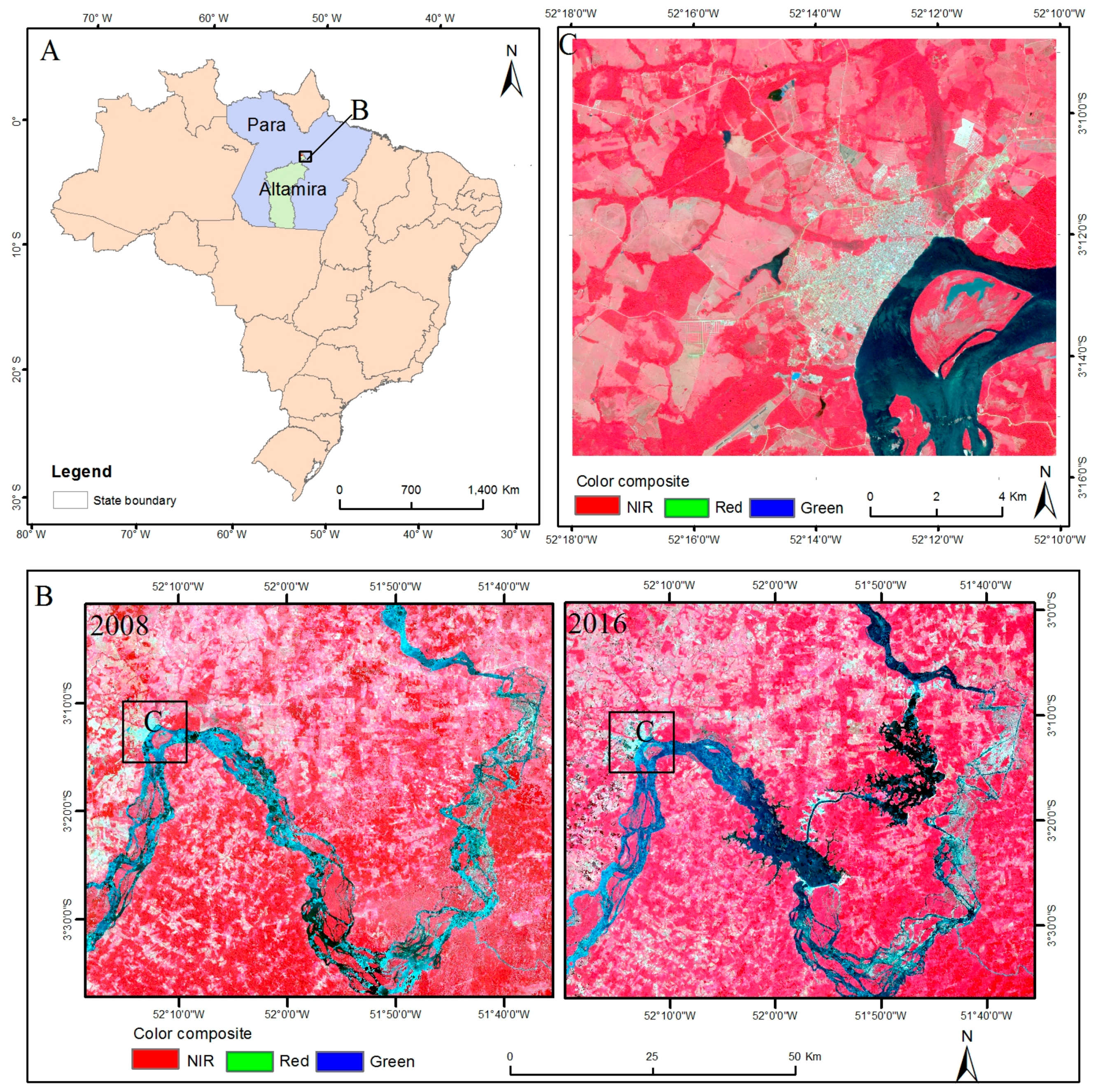
2. Study Area
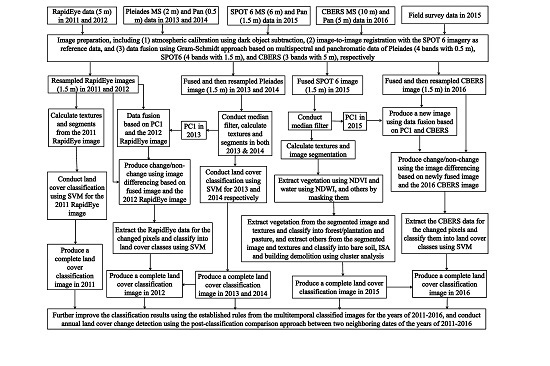
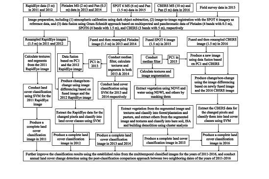
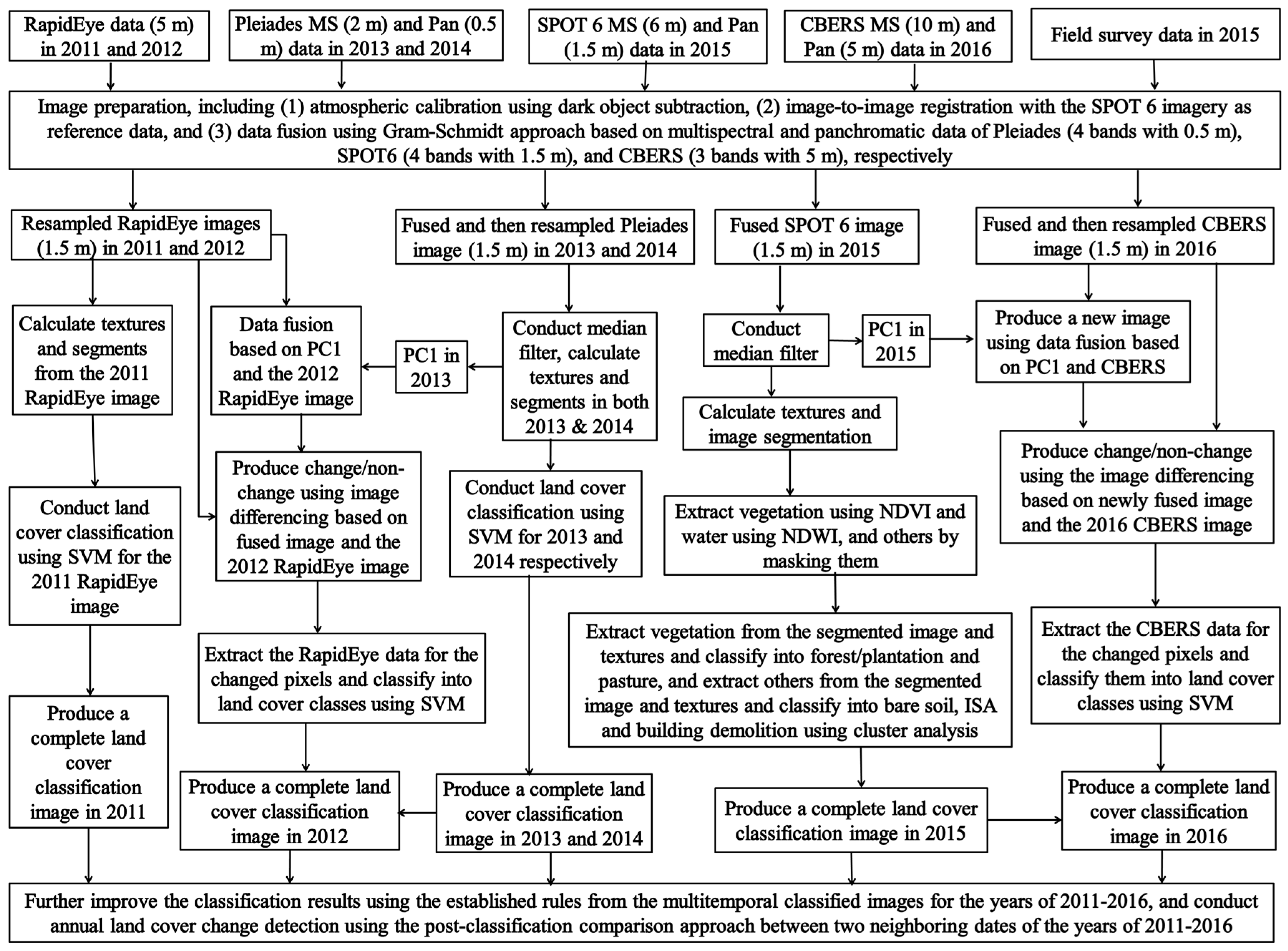
3. Materials and Methods
3.1. Data Collection and Preprocessing
3.2. Urban land-Cover Classification
3.3. Urban Land-Cover Change Detection
3.4. Accuracy Assessment
4. Results
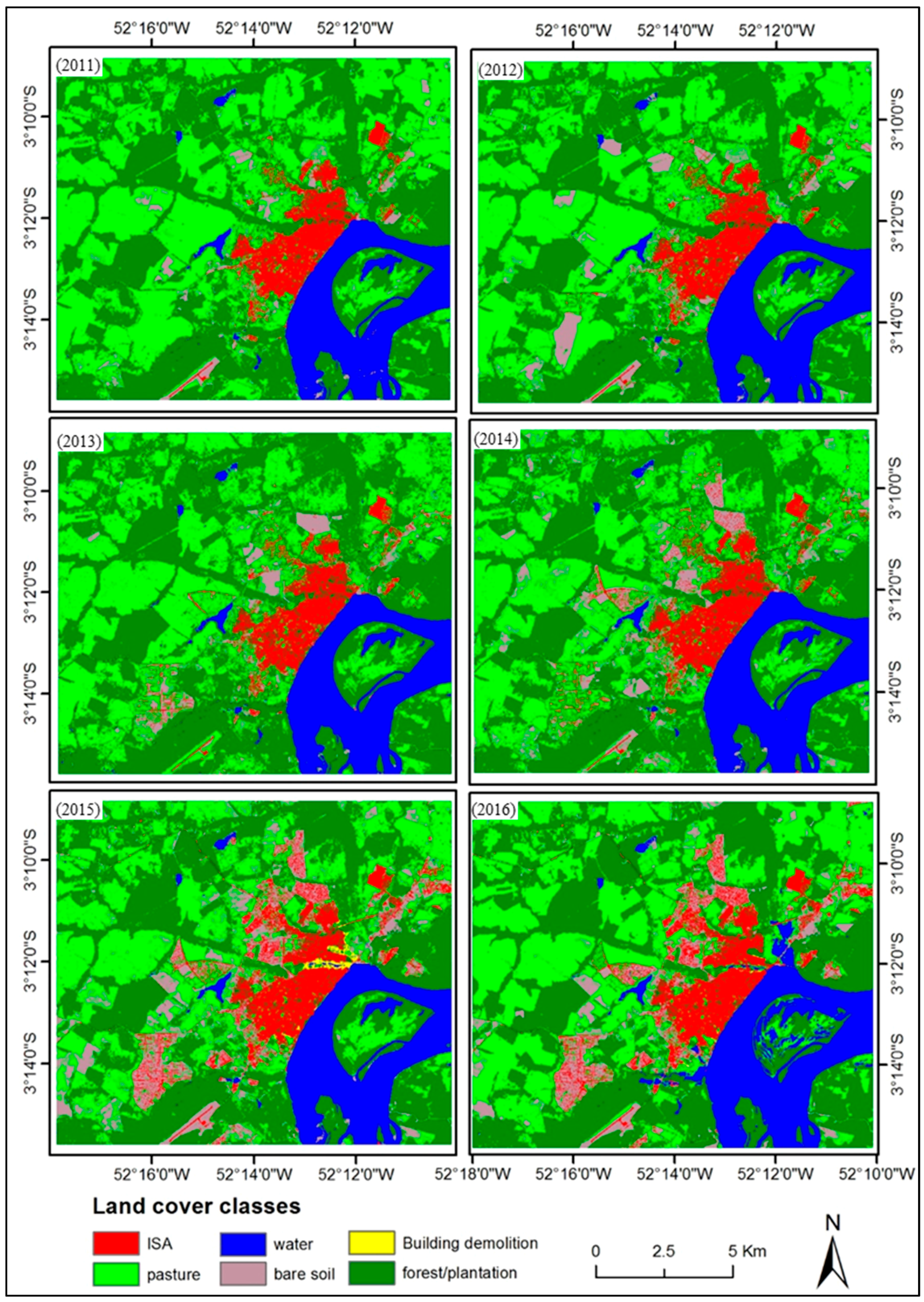
4.1. Analysis of Urban Land-Cover Distribution and Dynamic Changes
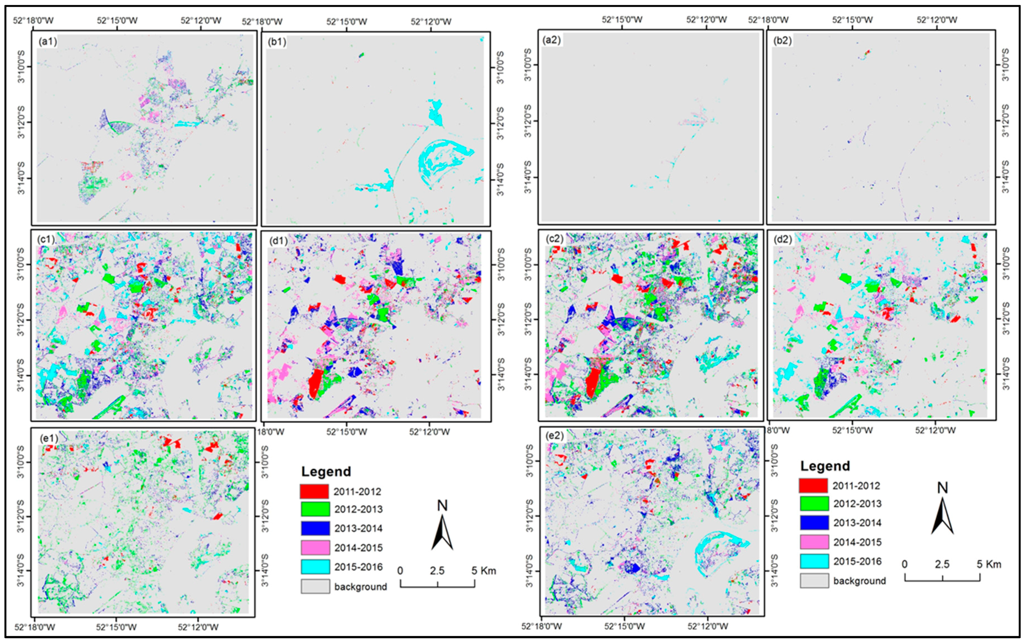
4.2. Analysis of Urban Land-Cover Change Trajectories
4.3. The Impacts of Belo Monte Dam Construction on Altamira’s Urban Land-Cover Change
5. Discussion
6. Conclusions
Acknowledgments
Author Contributions
Conflicts of Interest
References
- Fearnside, P.M. Dams in the Amazon: Belo Monte and Brazil’s Hydroeletric Development of the Xingu River Basin. Environ. Manag. 2006, 38, 16–27. [Google Scholar] [CrossRef] [PubMed]
- Santos, S.M.S.B.M.; Hernandez, F.M. (Eds.) Painel de Especialistas: Análise Crítica do Estudo de Impacto Ambiental do Aproveitamento Hidrelétrico de Belo Monte. Belém, Brazil. 2009. Available online: https://www.internationalrivers.org/sites/default/files/attached-files/belo_monte_pareceres_ibama_online_3.pdf (accessed on 19 April 2017).
- Rosenberg, D.M.; Berkes, F.; Bodaly, R.A.; Hecky, R.E.; Kelly, C.A.; Rudd, J.W.M. Large-scale impacts of hydroelectric development. Environ. Rev. 1997, 5, 27–54. [Google Scholar] [CrossRef]
- Lu, D.; Weng, Q. A survey of image classification methods and techniques for improving classification performance. Int. J. Remote Sens. 2007, 28, 823–870. [Google Scholar] [CrossRef]
- Lu, D.; Batistella, M.; Li, G.; Moran, E.; Hetrick, S.; Freitas, C.; Dutra, L.; Sant’Anna, S.J.S. Land use/cover classification in the Brazilian Amazon using satellite images. Braz. J. Agric. Res. 2012, 47, 1185–1208. [Google Scholar] [CrossRef] [PubMed]
- Zhu, Z.; Woodcock, C.E. Continuous change detection and classification of land cover using all available Landsat data. Remote Sens. Environ. 2014, 144, 152–171. [Google Scholar] [CrossRef]
- Asner, G.P. Cloud cover in Landsat observations of the Brazilian Amazon. Int. J. Remote Sens. 2001, 22, 3855–3862. [Google Scholar] [CrossRef]
- Lu, D.; Hetrick, S.; Moran, E.; Li, G. Application of time series Landsat images to examining land use/cover dynamic change. Photogramm. Eng. Remote Sens. 2012, 78, 747–755. [Google Scholar] [CrossRef]
- Lu, D.; Li, G.; Moran, E. Current situation and needs of change detection techniques. Int. J. Image Data Fusion 2014, 5, 13–38. [Google Scholar] [CrossRef]
- Singh, A. Digital change detection techniques using remotely-sensed data. Int. J. Remote Sens. 1989, 10, 989–1003. [Google Scholar] [CrossRef]
- Hansen, M.C.; Loveland, T.R. A review of large area monitoring of land cover change using Landsat data. Remote Sens. Environ. 2012, 122, 66–74. [Google Scholar] [CrossRef]
- Lu, D.; Li, G.; Moran, E.; Batistella, M.; Freitas, C. Mapping impervious surfaces with the integrated use of Landsat Thematic Mapper and radar data: A case study in an urban-rural landscape in the Brazilian Amazon. ISPRS J. Photogramm. Remote Sens. 2011, 66, 798–808. [Google Scholar] [CrossRef]
- Lu, D.; Moran, E.; Hetrick, S. Detection of impervious surface change with multitemporal Landsat images in an urban-rural frontier. ISPRS J. Photogramm. Remote Sens. 2011, 66, 298–306. [Google Scholar] [CrossRef] [PubMed]
- Lu, D.; Hetrick, S.; Moran, E.; Li, G. Detection of urban expansion in an urban-rural landscape with multitemporal QuickBird images. J. Appl. Remote Sens. 2010, 4, 041880. [Google Scholar] [CrossRef] [PubMed]
- Lu, D.; Hetrick, S.; Moran, E. Land cover classification in a complex urban-rural Landscape with QuickBird imagery. Photogramm. Eng. Remote Sens. 2010, 76, 1159–1168. [Google Scholar] [CrossRef]
- Su, W.; Li, J.; Chen, Y.; Liu, Z.; Zhang, J.; Low, T.M.; Suppiah, I.; Hashim, S.A.M. Textural and local spatial statistics for the object-oriented classification of urban areas using high resolution imagery. Int. J. Remote Sens. 2008, 29, 3105–3117. [Google Scholar] [CrossRef]
- Reis, M.; Dutra, L.V.; Sant’anna, S.; Escada, M. Examining multi-legend change detection in Amazon with pixel and region based methods. Remote Sens. 2017, 9, 77. [Google Scholar] [CrossRef]
- Dos Santos, J.A.; Gosselin, P.H.; Philipp-Foliguet, S.; Torres, R.D.S.; Falcao, A.X. Interactive multiscale classification of high-resolution remote sensing images. IEEE J. Sel. Top. Appl. Earth Obs. Remote Sens. 2013, 6, 2020–2034. [Google Scholar] [CrossRef]
- Myint, S.W.; Gober, P.; Brazel, A.; Grossman-Clarke, S.; Weng, Q. Per-pixel vs. object-based classification of urban land cover extraction using high spatial resolution imagery. Remote Sens. Environ. 2011, 115, 1145–1161. [Google Scholar] [CrossRef]
- Robertson, L.D.; King, D.J. Comparison of pixel- and object-based classification in land cover change mapping. Int. J. Remote Sens. 2011, 32, 1505–1529. [Google Scholar] [CrossRef]
- Gao, Y.; Mas, J.F.; Maathuis, B.H.P.; Zhang, X.; Van Dijk, P.M. Comparison of pixel-based and object-oriented image classification approaches—A case study in a coal fire area, Wuda, Inner Mongolia, China. Int. J. Remote Sens. 2006, 27, 4039–4055. [Google Scholar] [CrossRef]
- Huang, X.; Zhang, L. An SVM ensemble approach combining spectral, structural, and semantic features for the classification of high-resolution remotely sensed imagery. IEEE Trans. Geosci. Remote Sens. 2013, 51, 257–272. [Google Scholar] [CrossRef]
- Demir, B.; Bruzzone, L. Histogram-based attribute profiles for classification of very high resolution remote sensing images. IEEE Trans. Geosci. Remote Sens. 2016, 54, 2096–2107. [Google Scholar] [CrossRef]
- Qian, Y.; Zhou, W.; Yan, J.; Li, W.; Han, L. Comparing machine learning classifiers for object-based land cover classification using very high resolution imagery. Remote Sens. 2014, 7, 153–168. [Google Scholar] [CrossRef]
- Coppin, P.; Jonckheere, I.; Nackaerts, K.; Muys, B.; Lambin, E. Digital change detection methods in ecosystem monitoring: A review. Int. J. Remote Sens. 2004, 25, 1565–1596. [Google Scholar] [CrossRef]
- Hussain, M.; Chen, D.; Cheng, A.; Wei, H.; Stanley, D. Change detection from remotely sensed images: From pixel-based to object-based approaches. ISPRS J. Photogramm. Remote Sens. 2013, 80, 91–106. [Google Scholar] [CrossRef]
- Lu, D.; Mausel, P.; Brondízio, E.; Moran, E. Change detection techniques. Int. J. Remote Sens. 2004, 25, 2365–2407. [Google Scholar] [CrossRef]
- Chen, Y.; Lu, D.; Luo, G.; Huang, J. Detection of vegetation abundance change in the alpine tree line using multitemporal Landsat Thematic Mapper imagery. Int. J. Remote Sens. 2015, 36, 4683–4701. [Google Scholar] [CrossRef]
- Huang, C.; Goward, S.N.; Masek, J.G.; Thomas, N.; Zhu, Z.; Vogelmann, J.E. An automated approach for reconstructing recent forest disturbance history using dense Landsat time series stacks. Remote Sens. Environ. 2010, 114, 183–198. [Google Scholar] [CrossRef]
- Lu, D.; Li, G.; Moran, E.; Hetrick, S. Spatiotemporal analysis of land-use and land-cover change in the Brazilian Amazon. Int. J. Remote Sens. 2013, 34, 5953–5978. [Google Scholar] [CrossRef] [PubMed]
- Calvi, M.F. Fatores de adoção de sistemas agroflorestais por agricultores familiares do município de Medicilândia, Pará. Núcleo de Ciências Agrárias e Desenvolvimento Rural. Dissertação de Mestrado, Universidade Federal do Pará, Belém, Brazil, 2009. (In Portuguese). [Google Scholar]
- Moran, E.F. Developing the Amazon; Indiana University Press: Bloomington, IN, USA, 1981. [Google Scholar]
- PMA. Estimativa da População Urbana de Altamira a Partir do Acesso aos Serviços Médico-Hospitalares; Prefeitura Municipal de Altamira: Altamira, Brazil, 2013. [Google Scholar]
- Leturcq, G. Differences and similarities in impacts of hydroeletric dams between North and South of Brazil. Ambient. Soc. 2016, 19, 265–286. [Google Scholar] [CrossRef]
- ELETROBRÁS. Estudo de Impacto Ambiental—EIA. Relatório de Impacto Ambiental da Usina Hidrelétrica de Belo Monte—RIMA Belo Monte; Eletrobrás: Rio de Janeiro, Brazil, 2009. [Google Scholar]
- Chander, G.; Markham, B.L.; Helder, D.L. Summary of current radiometric calibration coefficients for Landsat MSS, TM, ETM+, and EO-1 ALI sensors. Remote Sens. Environ. 2009, 113, 893–903. [Google Scholar] [CrossRef]
- Chavez, P.S., Jr. Image-based atmospheric corrections: Revisited and improved. Photogramm. Eng. Remote Sens. 1996, 62, 1025–1036. [Google Scholar]
- Pohl, C.; van Genderen, J.L. Multisensor image fusion in remote sensing: Concepts, methods, and applications. Int. J. Remote Sens. 1998, 19, 823–854. [Google Scholar] [CrossRef]
- Zhang, J. Multisource remote sensing data fusion: Status and trends. Int. J. Image Data Fusion 2010, 1, 5–24. [Google Scholar] [CrossRef]
- Lu, D.; Li, G.; Moran, E.; Dutra, L.; Batistella, M. A comparison of multisensor integration methods for land-cover classification in the Brazilian Amazon. GISci. Remote Sens. 2011, 48, 345–370. [Google Scholar] [CrossRef]
- Liu, J.G. Smoothing Filter-based Intensity Modulation: A spectral preserve image fusion technique for improving spatial details. Int. J. Remote Sens. 2000, 21, 3461–3472. [Google Scholar] [CrossRef]
- Karathanassi, V.; Kolokousis, P.; Ioannidou, S. A comparison study on fusion methods using evaluation indicators. Int. J. Remote Sens. 2007, 28, 2309–2341. [Google Scholar] [CrossRef]
- Laben, C.A.; Brower, B.V. Process for Enhancing the Spatial Resolution of Multispectral Imagery Using Pan-Sharpening. U.S. Patent No. 6011875, 4 January 2000. [Google Scholar]
- Haralick, R.M.; Shanmugam, K. Textural features for image classification. IEEE Trans. Syst. Man Cybern. 1973, 3, 610–621. [Google Scholar] [CrossRef]
- Lu, D.; Li, G.; Moran, E.; Dutra, L.; Batistella, M. The roles of textural images in improving land-cover classification in the Brazilian Amazon. Int. J. Remote Sens. 2014, 35, 8188–8207. [Google Scholar] [CrossRef]
- Laurin, G.V.; Liesenberg, V.; Chen, Q.; Guerriero, L.; Del Frate, F.; Bartolini, A.; Coomes, D.; Wilebore, B.; Lindsell, J.; Valentini, R. Optical and SAR sensor synergies for forest and land cover mapping in a tropical site in West Africa. Int. J. Appl. Earth Obs. Geoinf. 2013, 21, 7–16. [Google Scholar] [CrossRef]
- Dey, V.; Zhang, Y.; Zhong, M.; Salehi, B. Image segmentation techniques for urban land cover segmentation of VHR imagery: Recent developments and future prospects. Int. J. Geoinf. 2013, 9, 15–35. [Google Scholar]
- Zhang, L.; Jia, K.; Li, X.; Yuan, Q.; Zhao, X. Multi-scale segmentation approach for object-based land-cover classification using high-resolution imagery. Remote Sens. Lett. 2014, 5, 73–82. [Google Scholar] [CrossRef]
- Li, W.; Saphores, J.D.M.; Gillespie, T.W. A comparison of the economic benefits of urban green spaces estimated with NDVI and with high-resolution land cover data. Landsc. Urban Plan. 2015, 133, 105–117. [Google Scholar] [CrossRef]
- Odindi, J.O.; Mhangara, P. Green spaces trends in the city of Port Elizabeth from 1990 to 2000 using remote sensing. Int. J. Environ. Res. 2012, 6, 653–662. [Google Scholar]
- McFeeters, S.K. The use of the Normalized Difference Water Index (NDWI) in the delineation of open water features. Int. J. Remote Sens. 1996, 17, 1425–1432. [Google Scholar] [CrossRef]
- Thakkar, A.; Desai, V.; Patel, A.; Potdar, M. Land use/land cover classification using remote sensing data and derived indices in a heterogeneous landscape of a khan-kali watershed, Gujarat. Asian J. Geoinf. 2015, 14, 1–12. [Google Scholar]
- Adam, E.; Mutanga, O.; Odindi, J.; Abdel-Rahman, E.M. Land-use/cover classification in a heterogeneous coastal landscape using RapidEye imagery: Evaluating the performance of random forest and support vector machines classifiers. Int. J. Remote Sens. 2014, 35, 3440–3458. [Google Scholar] [CrossRef]
- Banerjee, B.; Bhattacharya, A.; Buddhiraju, K.M. A generic land-cover classification framework for polarimetric SAR images using the optimum Touzi decomposition parameter subset—An insight on mutual information-based feature selection techniques. IEEE J. Sel. Top. Appl. Earth Obs. Remote Sens. 2014, 7, 1167–1176. [Google Scholar] [CrossRef]
- Congalton, R.G.; Green, K. Assessing the Accuracy of Remotely Sensed Data: Principles and Practices, 2nd ed.; CRC Press: Boca Raton, FL, USA, 2008. [Google Scholar]
- Foody, G.M. Status of land cover classification accuracy assessment. Remote Sens. Environ. 2002, 80, 185–201. [Google Scholar] [CrossRef]
- Li, G.; Lu, D.; Moran, E.; Sant’Anna, S.J.S. A comparative analysis of classification algorithms and multiple sensor data for land use/land cover classification in the Brazilian Amazon. J. Appl. Remote Sens. 2012, 6. [Google Scholar] [CrossRef]
- Angelis, C.F.; Freitas, C.D.C.; Valeriano, D.M.; Dutra, L.V. Multitemporal analysis of land use/land cover JERS-1 backscatter in the Brazilian Tropical Rainforest. Int. J. Remote Sens. 2002, 23, 1231–1240. [Google Scholar] [CrossRef]
- Anjos, D.S.; Lu, D.; Dutra, L.V.; Sant’anna, S.J.S. Change detection techniques using multisensor data. In Remotely Sensed Data Characterization, Classification, and Accuracies; Thenkabail, P.S., Ed.; CRC Press: Boca Raton, FL, USA, 2016; pp. 377–397. [Google Scholar]
- Lu, D.; Batistella, M.; Moran, E. Integration of Landsat TM and SPOT HRG images for vegetation change detection in the Brazilian Amazon. Photogramm. Eng. Remote Sens. 2008, 74, 421–430. [Google Scholar] [CrossRef]
- Zhou, W.; Troy, A.; Grove, J.M. Object-based land cover classification and change analysis in the Baltimore metropolitan area using multi-temporal high resolution remote sensing data. Sensors 2008, 8, 1613–1636. [Google Scholar] [CrossRef] [PubMed]
- Chen, G.; Hay, G.J.; Carvalho, L.M.T.; Wulder, M.A. Object-based change detection. Int. J. Remote Sens. 2012, 33, 4434–4457. [Google Scholar] [CrossRef]
- Zeng, Y.; Zhang, J.; van Genderen, J.L.; Zhang, Y. Image fusion for land cover change detection. Int. J. Image Data Fusion 2010, 1, 193–215. [Google Scholar] [CrossRef]
- Chen, D.; Stow, D.A.; Gong, P. Examining the effect of spatial resolution and texture window size on classification accuracy: An urban environment case. Int. J. Remote Sens. 2004, 25, 2177–2192. [Google Scholar] [CrossRef]


| RapidEye | Pleiades | SPOT 6 | CBERS | |
|---|---|---|---|---|
| Spectral bands | 440–510 nm (B) 520–590 nm (G) 630–685 nm (R) 690–730 nm (R Edge) 760–850 nm (NIR) | 480–830 nm (Pan) 430–550 nm (B) 490–610 nm (G) 600–720 nm (R) 750–950 nm(NIR) | 450–745 nm (Pan) 450–525 nm (B) 530–590 nm (G) 625–695 nm (R) 760–890 nm (NIR) | 510–850 nm (Pan) 520–590 nm (G) 630–690 nm (R) 770–890 nm (NIR) |
| Spatial resolution | Ground sampling distance (nadir): 6.5 m Pixel size: 5 m | Pan: 0.5 m MS (B, G, R, NIR): 2.0 m | Pan: 1.5 m MS (B, G, R, NIR): 6.0 m | Pan: 5 m MS (G, R, NIR): 10 m |
| Image acquisition date | 28 July 2011 1 August 2012 | 13 July 2013 18 July 2014 | 19 August 2015 | 3 July 2016 |
| Year | Type | Reference Data | Overall Accuracy | ||||||||||
|---|---|---|---|---|---|---|---|---|---|---|---|---|---|
| ISA | BD | W | PA | BS | F/PL | CT | RT | UA | PA | ||||
| Classified data | 2011 | ISA | 15 | 0 | 0 | 1 | 2 | 2 | 20 | 17 | 75.0 | 88.2 | OA = 90.0%; KC = 0.85 |
| BD | 0 | 0 | 0 | 0 | 0 | 0 | 0 | 0 | 0 | 0 | |||
| W | 0 | 0 | 32 | 0 | 0 | 0 | 32 | 32 | 100.0 | 100.0 | |||
| PA | 2 | 0 | 0 | 112 | 0 | 12 | 126 | 124 | 88.9 | 90.3 | |||
| BS | 0 | 0 | 0 | 7 | 9 | 0 | 16 | 11 | 56.3 | 81.8 | |||
| F/PL | 0 | 0 | 0 | 4 | 0 | 102 | 106 | 116 | 96.2 | 87.9 | |||
| 2012 | ISA | 16 | 0 | 0 | 0 | 1 | 0 | 17 | 17 | 94.1 | 94.1 | OA = 90.7%; KC = 0.86 | |
| BD | 0 | 0 | 0 | 0 | 0 | 0 | 0 | 0 | 0 | 0 | |||
| W | 0 | 0 | 32 | 0 | 0 | 0 | 32 | 32 | 100.0 | 100.0 | |||
| PA | 0 | 0 | 0 | 98 | 1 | 10 | 109 | 109 | 89.9 | 89.9 | |||
| BS | 1 | 0 | 0 | 4 | 14 | 4 | 23 | 16 | 60.9 | 87.5 | |||
| F/PL | 0 | 0 | 0 | 7 | 0 | 112 | 119 | 126 | 94.1 | 88.9 | |||
| 2013 | ISA | 17 | 0 | 0 | 0 | 1 | 0 | 18 | 18 | 94.4 | 94.4 | OA = 91.7%; KC = 0.88 | |
| BD | 0 | 0 | 0 | 0 | 0 | 0 | 0 | 0 | 0 | 0 | |||
| W | 0 | 0 | 33 | 0 | 0 | 0 | 33 | 33 | 100.0 | 100.0 | |||
| PA | 0 | 0 | 0 | 94 | 1 | 13 | 108 | 103 | 87.0 | 91.3 | |||
| BS | 1 | 0 | 0 | 2 | 12 | 0 | 15 | 14 | 80.0 | 85.7 | |||
| F/PL | 0 | 0 | 0 | 7 | 0 | 119 | 126 | 132 | 94.4 | 90.2 | |||
| 2014 | ISA | 19 | 0 | 0 | 2 | 0 | 0 | 21 | 20 | 90.5 | 95.0 | OA = 91.3%; KC = 0.88 | |
| BD | 0 | 0 | 0 | 0 | 0 | 0 | 0 | 0 | 0 | 0 | |||
| W | 0 | 0 | 31 | 0 | 0 | 0 | 31 | 32 | 100.0 | 96.9 | |||
| PA | 0 | 0 | 0 | 87 | 5 | 6 | 98 | 99 | 88.8 | 87.9 | |||
| BS | 1 | 0 | 0 | 1 | 21 | 1 | 24 | 26 | 87.5 | 80.8 | |||
| F/PL | 0 | 0 | 1 | 9 | 0 | 116 | 126 | 123 | 92.1 | 94.3 | |||
| 2015 | ISA | 23 | 0 | 0 | 0 | 0 | 1 | 24 | 24 | 95.8 | 95.8 | OA = 92.3%; KC = 0.90 | |
| BD | 0 | 6 | 0 | 0 | 0 | 0 | 6 | 6 | 100.0 | 100.0 | |||
| W | 0 | 0 | 32 | 0 | 0 | 0 | 32 | 32 | 100.0 | 100.0 | |||
| PA | 1 | 0 | 0 | 75 | 2 | 6 | 83 | 87 | 90.4 | 86.2 | |||
| BS | 0 | 0 | 0 | 1 | 33 | 1 | 35 | 35 | 94.3 | 94.3 | |||
| F/PL | 0 | 0 | 0 | 11 | 1 | 108 | 120 | 116 | 90.0 | 93.1 | |||
| 2016 | ISA | 20 | 0 | 0 | 0 | 0 | 1 | 21 | 25 | 95.2 | 80.0 | OA = 91.3%; KC = 0.88 | |
| BD | 0 | 3 | 0 | 0 | 0 | 0 | 3 | 4 | 100.0 | 75.0 | |||
| W | 0 | 0 | 36 | 0 | 1 | 0 | 37 | 36 | 97.3 | 100.0 | |||
| PA | 5 | 1 | 0 | 84 | 2 | 4 | 96 | 96 | 87.5 | 87.5 | |||
| BS | 0 | 0 | 0 | 3 | 24 | 0 | 27 | 27 | 88.9 | 88.9 | |||
| F/PL | 0 | 0 | 0 | 9 | 0 | 107 | 116 | 112 | 92.2 | 95.5 | |||
| Area (km2) of Each Land Cover in Various Years | ||||||
|---|---|---|---|---|---|---|
| Land Cover | 2011 | 2012 | 2013 | 2014 | 2015 | 2016 |
| ISA | 10.45 | 10.58 | 10.98 | 12.54 | 14.79 | 15.33 |
| W | 19.34 | 19.43 | 19.71 | 19.38 | 19.47 | 23.65 |
| PA | 68.45 | 63.88 | 60.87 | 57.62 | 52.27 | 57.22 |
| BS | 6.55 | 9.88 | 8.28 | 15.51 | 21.03 | 14.55 |
| F/PL | 73.15 | 74.15 | 78.09 | 72.88 | 69.76 | 67.1 |
| BD | 0.61 | 0.09 | ||||
| Percent (%) of Each Land Cover Accounting for Total Area | ||||||
| Land Cover | 2011 | 2012 | 2013 | 2014 | 2015 | 2016 |
| ISA | 5.87 | 5.95 | 6.17 | 7.05 | 8.31 | 8.62 |
| W | 10.87 | 10.92 | 11.08 | 10.89 | 10.94 | 13.29 |
| PA | 38.47 | 35.9 | 34.21 | 32.38 | 29.38 | 32.16 |
| BS | 3.68 | 5.55 | 4.65 | 8.72 | 11.82 | 8.18 |
| F/PL | 41.11 | 41.68 | 43.89 | 40.96 | 39.21 | 37.71 |
| BD | 0.34 | 0.05 | ||||
| Type | 2011–2016 (km2) | Changed Area (km2) of Land Covers in One-Year Periods | ||||
|---|---|---|---|---|---|---|
| 2011–2012 | 2012–2013 | 2013–2014 | 2014–2015 | 2015–2016 | ||
| ISA | 4.88 | 0.13 | 0.40 | 1.56 | 2.25 | 0.54 |
| W | 4.31 | 0.09 | 0.28 | −0.33 | 0.09 | 4.18 |
| PA | −11.23 | −4.57 | −3.01 | −3.25 | −5.35 | 4.95 |
| BS | 8.00 | 3.33 | −1.60 | 7.23 | 5.52 | −6.48 |
| F/PL | −6.05 | 1.00 | 3.94 | −5.21 | −3.12 | −2.66 |
| BD | 0.09 | 0.61 | −0.52 | |||
| Type | 2011–2016 (%) | Percent (%) of Each Changed Land Cover Accounting for Total Changed Area | ||||
| 2011–2012 | 2012–2013 | 2013–2014 | 2014–2015 | 2015–2016 | ||
| ISA | 14.12 | 1.43 | 4.33 | 8.87 | 13.28 | 2.79 |
| W | 12.47 | 0.99 | 3.03 | 1.88 | 0.53 | 21.62 |
| PA | −32.49 | −50.11 | −32.61 | −18.49 | −31.58 | 25.61 |
| BS | 23.15 | 36.51 | −17.33 | 41.13 | 32.59 | −33.52 |
| F/PL | −17.51 | 10.96 | 42.69 | −29.64 | −18.42 | −13.76 |
| BD | 0.26 | 3.60 | −2.69 | |||
| Land-Cover Change Trajectories | 2011–2016 | 2011–2012 | 2012–2013 | 2013–2014 | 2014–2015 | 2015–2016 | |
|---|---|---|---|---|---|---|---|
| ISA change | PA-ISA | 4.00 | 0.33 | 1.09 | 1.70 | 0.48 | 0.11 |
| BS-ISA | 0.63 | 0.09 | 0.51 | 0.39 | 1.09 | 0.43 | |
| Non(PA, BS)-ISA | 1.56 | 0 | 0.01 | 0.02 | 0.01 | 0.19 | |
| Gain | 6.19 | 0.42 | 1.61 | 2.11 | 1.58 | 0.73 | |
| ISA-BD | 0.09 | 0 | 0.00 | 0.00 | 0.61 | 0.09 | |
| ISA-Non(BD) | 0.79 | 0.01 | 0.02 | 0 | 0.03 | 0.12 | |
| Loss | 0.88 | 0.01 | 0.02 | 0 | 0.64 | 0.21 | |
| Water change | BS-W | 0.57 | 0.10 | 0.12 | 0 | 0.02 | 0.58 |
| Non(BS)-W | 3.89 | 0.05 | 0.13 | 0.06 | 0.03 | 3.62 | |
| Gain | 4.46 | 0.15 | 0.25 | 0.06 | 0.05 | 4.20 | |
| W-BS | 0.02 | 0.04 | 0.01 | 0.14 | 0.03 | 0.01 | |
| W-Non(BS) | 0.07 | 0.01 | 0.06 | 0.12 | 0.06 | 0.01 | |
| Loss | 0.09 | 0.05 | 0.07 | 0.26 | 0.09 | 0.02 | |
| Pasture change | BS-PA | 2.32 | 1.28 | 5.53 | 2.6 | 4.58 | 6.41 |
| F/PL-PA | 5.56 | 1.10 | 4.01 | 7.55 | 3.67 | 1.99 | |
| Non(BS, F/PL)-PA | 0.39 | 0.01 | 0.05 | 0.10 | 0.05 | 0.31 | |
| Gain | 8.27 | 2.39 | 9.59 | 10.25 | 8.30 | 8.71 | |
| PA-BS | 10.54 | 4.70 | 4.40 | 8.27 | 11.57 | 0.82 | |
| PA-F/PL | 3.54 | 1.67 | 7.71 | 4.10 | 1.60 | 1.45 | |
| PA-Non(BS, F/PL) | 1.45 | 0.37 | 1.20 | 1.76 | 0.48 | 1.68 | |
| Loss | 15.53 | 6.74 | 13.31 | 14.13 | 13.65 | 3.95 | |
| Bare soil change | PA-BS | 10.54 | 4.70 | 4.40 | 8.27 | 11.57 | 0.82 |
| Non(PA)-BS | 1.52 | 0.19 | 0.42 | 1.88 | 0.13 | 0.26 | |
| Gain | 12.06 | 4.89 | 4.82 | 10.15 | 11.70 | 1.08 | |
| BS-PA | 2.32 | 1.28 | 5.53 | 2.60 | 4.58 | 6.41 | |
| BS-F/PL | 0.39 | 0.42 | 0.50 | 0.22 | 0.38 | 0.09 | |
| BS-Non(PA, F/PL) | 1.20 | 0.19 | 0.63 | 0.39 | 1.11 | 1.01 | |
| Loss | 3.91 | 1.89 | 6.66 | 3.21 | 6.07 | 7.51 | |
| Forest/plantation change | PA-F/PL | 3.54 | 1.67 | 7.71 | 4.10 | 1.60 | 1.45 |
| Non(PA)-F/PL | 0.39 | 0.42 | 0.50 | 0.22 | 0.38 | 0.09 | |
| Gain | 3.93 | 2.09 | 8.21 | 4.32 | 1.98 | 1.54 | |
| F/PL-PA | 5.56 | 1.10 | 4.01 | 7.55 | 3.67 | 1.99 | |
| F/PL-Non(PA) | 5.04 | 0.15 | 0.41 | 1.74 | 0.10 | 2.23 | |
| Loss | 10.60 | 1.25 | 4.42 | 9.29 | 3.77 | 4.22 | |
| Type | Area (km2) | Annual Average Changed Area (km2/Year) | Annual Average Changed Area Rate (%) | |||||||
|---|---|---|---|---|---|---|---|---|---|---|
| 1991 | 2000 | 2011 | 2016 | 2000–1991 | 2011–2000 | 2016–2011 | 2000–1991 | 2011–2000 | 2016–2011 | |
| FP | 80.10 | 82.19 | 73.21 | 67.07 | 0.23 | −0.82 | −1.23 | 0.29 | −0.99 | −1.68 |
| PA | 65.99 | 63.17 | 65.83 | 57.40 | −0.31 | 0.24 | −1.69 | −0.47 | 0.38 | −2.56 |
| ISA | 12.11 | 12.72 | 13.13 | 15.38 | 0.07 | 0.04 | 0.45 | 0.56 | 0.29 | 3.43 |
| Water | 19.91 | 20.02 | 19.32 | 23.61 | 0.01 | −0.06 | 0.86 | 0.06 | −0.32 | 4.44 |
| Number of Persons | Annual Average Population Growth (Person/Year) | Annual Average Population Growth Rate (%) | ||||||||
| 1991 | 2000 | 2010 | 2012 | 2000–1991 | 2010–2000 | 2012–2010 | 2000–1991 | 2010–2000 | 2012–2010 | |
| Pop | 50,145 | 62,285 | 77,195 | 150,000 | 1349 | 1491 | 36,403 | 2.69 | 2.39 | 47.16 |
| Change Trajectories | Average Annual Changed Area (km2) | ||
|---|---|---|---|
| 1991–2000 | 2000–2011 | 2011–2016 | |
| Forest/plantation to Pasture | 1.92 | 1.94 | 1.11 |
| Forest/plantation to Bare soil | 0.24 | ||
| Forest/plantation to Water | 0.45 | ||
| Forest/plantation to ISA | 0.06 | 0.08 | 0.31 |
| Pasture to ISA | 0.12 | 0.13 | 0.46 |
© 2017 by the authors. Licensee MDPI, Basel, Switzerland. This article is an open access article distributed under the terms and conditions of the Creative Commons Attribution (CC BY) license (http://creativecommons.org/licenses/by/4.0/).
Share and Cite
Feng, Y.; Lu, D.; Moran, E.F.; Dutra, L.V.; Calvi, M.F.; De Oliveira, M.A.F. Examining Spatial Distribution and Dynamic Change of Urban Land Covers in the Brazilian Amazon Using Multitemporal Multisensor High Spatial Resolution Satellite Imagery. Remote Sens. 2017, 9, 381. https://0-doi-org.brum.beds.ac.uk/10.3390/rs9040381
Feng Y, Lu D, Moran EF, Dutra LV, Calvi MF, De Oliveira MAF. Examining Spatial Distribution and Dynamic Change of Urban Land Covers in the Brazilian Amazon Using Multitemporal Multisensor High Spatial Resolution Satellite Imagery. Remote Sensing. 2017; 9(4):381. https://0-doi-org.brum.beds.ac.uk/10.3390/rs9040381
Chicago/Turabian StyleFeng, Yunyun, Dengsheng Lu, Emilio F. Moran, Luciano Vieira Dutra, Miquéias Freitas Calvi, and Maria Antonia Falcão De Oliveira. 2017. "Examining Spatial Distribution and Dynamic Change of Urban Land Covers in the Brazilian Amazon Using Multitemporal Multisensor High Spatial Resolution Satellite Imagery" Remote Sensing 9, no. 4: 381. https://0-doi-org.brum.beds.ac.uk/10.3390/rs9040381