Article

Extrapolating Forest Canopy Fuel Properties in the California Rim Fire by Combining Airborne LiDAR and Landsat OLI Data

1
Centre for Landscape and Climate Research, Department of Geography, University of Leicester, Leicester LE1 7RH, UK
2
Jet Propulsion Laboratory (JPL), California Institute of Technology, Pasadena, CA 91109, USA
3
The Climate Corporation, 201 Third Street, Suite 1100, San Francisco, CA 94103, USA
4
Center for Spatial Technologies and Remote Sensing (CSTARS), University of California Davis, Davis, CA 95618, USA
5
Region 5 Remote Sensing Lab, McClellan, USDA Forest Service, Vallejo, CA 95652, USA
6
National Centre for Earth Observation, University of Leicester, Leicester LE1 7RH, UK
*
Author to whom correspondence should be addressed.
Submission received: 8 March 2017 / Revised: 11 April 2017 / Accepted: 19 April 2017 / Published: 22 April 2017

Abstract

:
Accurate, spatially explicit information about forest canopy fuel properties is essential for ecosystem management strategies for reducing the severity of forest fires. Airborne LiDAR technology has demonstrated its ability to accurately map canopy fuels. However, its geographical and temporal coverage is limited, thus making it difficult to characterize fuel properties over large regions before catastrophic events occur. This study presents a two-step methodology for integrating post-fire airborne LiDAR and pre-fire Landsat OLI (Operational Land Imager) data to estimate important pre-fire canopy fuel properties for crown fire spread, namely canopy fuel load (CFL), canopy cover (CC), and canopy bulk density (CBD). This study focused on a fire prone area affected by the large 2013 Rim fire in the Sierra Nevada Mountains, California, USA. First, LiDAR data was used to estimate CFL, CC, and CBD across an unburned 2 km buffer with similar structural characteristics to the burned area. Second, the LiDAR-based canopy fuel properties were extrapolated over the whole area using Landsat OLI data, which yielded an R2 of 0.8, 0.79, and 0.64 and RMSE of 3.76 Mg·ha−1, 0.09, and 0.02 kg·m−3 for CFL, CC, and CBD, respectively. The uncertainty of the estimates was estimated for each pixel using a bootstrapping approach, and the 95% confidence intervals are reported. The proposed methodology provides a detailed spatial estimation of forest canopy fuel properties along with their uncertainty that can be readily integrated into fire behavior and fire effects models. The methodology could be also integrated into the LANDFIRE program to improve the information on canopy fuels.

Graphical Abstract

1. Introduction

Forest fuels, the organic matter available for fire ignition and combustion, are an essential component of fire management activities [1]. Accurate, spatially explicit information on forest fuels is required by fire behavior and effects models used in fire management decision support systems, such as BehavePlus Fire Modeling System, FlamMAP, or First Order Fire Effects Model (FOFEM).
Fire suppression policies adopted during the last century and demographic factors like rural abandonment have led to fuel accumulation and spatial homogenization of forest fuels that can unintentionally foster extreme fire events exceeding the recovery capacity of the ecosystems and reducing their resilience [2]. Moreover, these megafires can adversely change fundamental processes of energy exchange, water fluxes, and nutrient and carbon cycling [3]. Although historically rare, megafires are becoming more frequent worldwide, regardless of socio-economic and ecological conditions or fuel types [3]. Climate change projections indicate their frequency and intensity are expected to further increase as a result of longer and drier fire seasons [4].
Canopy fuels are particularly important in assessing fire risk because they represent the fuel layer supporting crown fire spread. Crown fires are more difficult to control than surface fires due to the increase in the rate of spread, intensity, and spotting, and their effects are more severe and lasting than surface fires [5]. Fuel properties commonly accepted to control crown fire spread are canopy cover (CC), canopy fuel load (CFL), and canopy bulk density (CBD) [6]. Canopy cover is defined as the proportion (0%–1% or 0%–100%) of the forest floor that is covered by the vertical projection of the tree crowns. This parameter characterizes the horizontal continuity of canopy fuels which affects the development and propagation of crown fires. CFL refers to the amount of fuel that is potentially available for combustion, expressed in kg·m−2 or Mg·ha−1. It can be represented by the foliage biomass [7,8,9] or by foliage plus the biomass of lichens, moss, and the proportion of small branches that would be consumed in the flaming front [5,7]. CBD, the mass of available canopy fuel per unit canopy volume (kg·m−3) that can burn in a crown fire, describes the density of the available canopy fuel in the stand and determines the critical spread rate needed to sustain an active crown fire [5].
Remote sensing technology, particularly LiDAR, can provide accurate spatio-temporal characterizations of forest canopy fuels due to their sensitivity to forest structure. LiDAR data collected from terrestrial, airborne and satellite sensors have already been successfully used to characterize canopy fuels [10,11,12,13]. For instance, CC has been accurately estimated using airborne LiDAR data in a wide range of ecosystems [14,15]. CFL has also been successfully estimated from metrics derived from the height distribution of the returns [12,13,16] given the correlation between vegetation height and biomass. Since CBD is essentially a three-dimensional (3D) variable that requires a description of the horizontal and vertical distributions of fuel through the canopy, the measurements of vegetation structure provided by LiDAR have proven to be the most suitable to estimate CBD [8,11,12,17]. A further description of the use of LiDAR technology to characterize forest fuels can be found in Gajardo et al. [18].
Most of the research on canopy fuel characterization with LiDAR data has been carried out using airborne sensors focusing on fine spatial scales and small geographical extents; however, information on forest fuels is required at multiple spatial scales in order to develop appropriate fire management decision-making activities [1]. In addition, the temporal coverage with airborne sensors is limited by cost of acquisition, which hampers the analysis of fuel dynamics. García et al. [11] demonstrated the capability of the ICESat/GLAS spaceborne LiDAR sensor to estimate canopy fuel properties. In the next few years, two spaceborne LiDAR missions are planned: the ICESat-2/ATLAS [19] and the Global Ecosystem Dynamics Investigation (GEDI) [20]. These multi-beam profilers will provide a dense sampling of the Earth’s terrestrial ecosystems, but they will not provide continuous coverage. Therefore, in order to provide large-scale estimates of canopy fuel properties from satellite LiDAR sensors or to extrapolate airborne LiDAR based estimates over larger geographical extents, it is necessary to develop methods for the integration of LiDAR and satellite sensors that provide better spatial coverage and temporal repeat frequency. In recent years, several studies have evaluated the use of multispectral and radar data to spatially extrapolate some biophysical variables estimated from LiDAR [21,22,23]. However, their potential to extrapolate LiDAR-based canopy fuel properties has not been evaluated.
Passive optical sensors, particularly Landsat, have been commonly used to estimate canopy fuel properties. They generally rely on empirical relationships between field estimates and the spectral information provided by the sensors [24,25]. The main limitation of passive sensors to characterize fuels is their limited sensitivity to vegetation height and vertical distribution. Therefore, while these studies successfully estimated CC, poorer results were obtained for CBD.
This research aimed at establishing a novel method for estimating important canopy fuel properties to characterize fire behavior and fire effects by integrating post-fire LiDAR and pre-fire Landsat OLI (hereafter termed Landsat) data. The specific objectives were to (1) estimate CFL, CC, and CBD from LiDAR data over unburned areas, (2) extrapolate these LiDAR-based estimates over the entire burned area based on a statistical approach using a Landsat image acquired shortly before the fire, (3) quantify the uncertainty associated with each pixel, and (4) evaluate the relationship between the variables estimated and the burn severity.

2. Materials and Methods
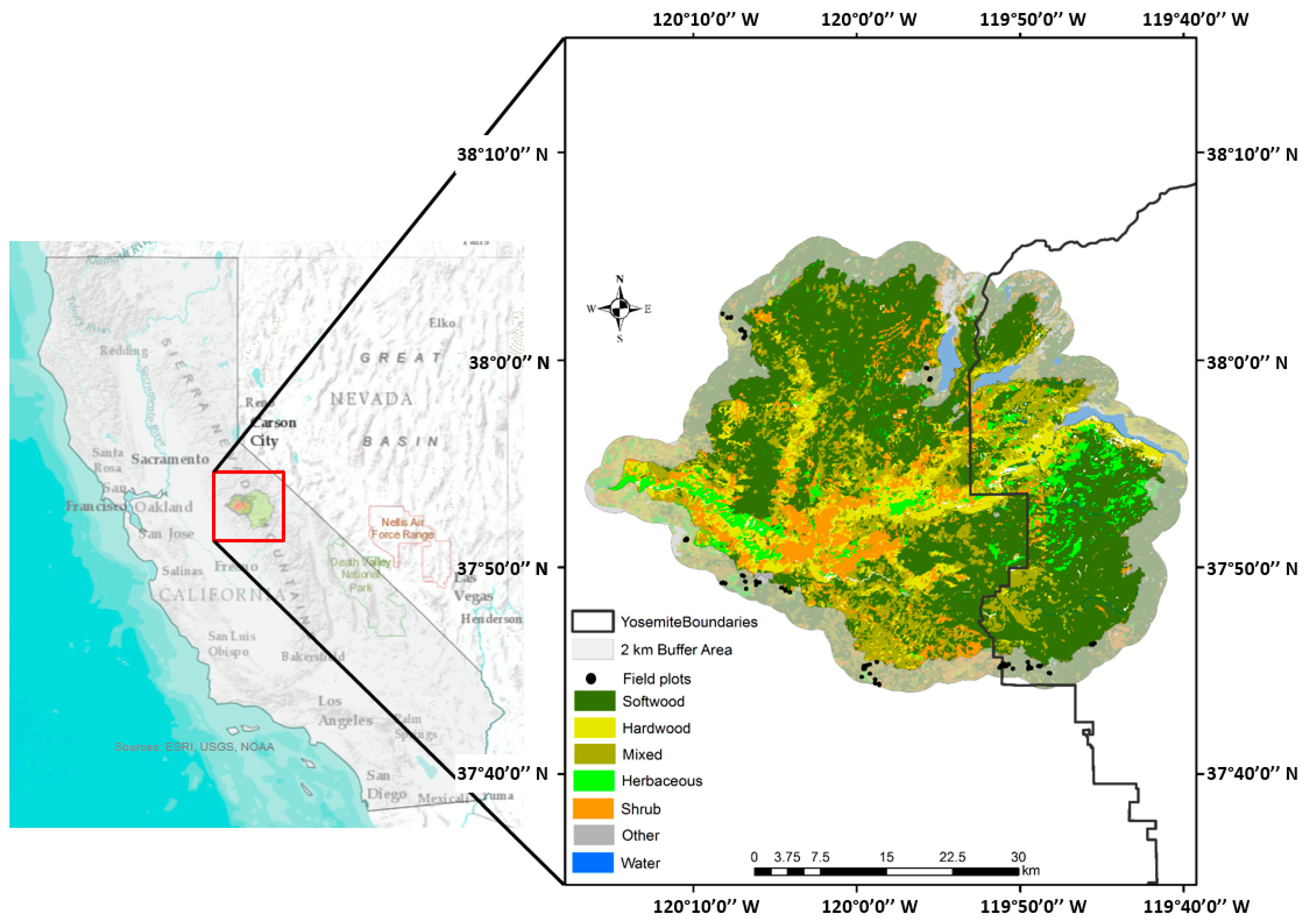
2.1. Study Area

The study site comprises the footprint of the 2013 Rim fire in the Sierra Nevada Mountains, California, that burned more than 104,000 ha over the Stanislaus National Forest and Yosemite National Park (Figure 1). The area presents rough topography with elevations ranging from 60 to 2400 m and slopes of up to 90%. The fire burned through a mosaic of vegetation types that vary with elevation, which included low-elevation grasslands, chaparral and foothill-oak woodland savanna habitat, mixed conifer-broadleaf forests dominated by pines in the lower montane zone, and mixed conifer forests in higher elevation areas dominated by firs. A more detailed description of the study site can be found in Casas et al. [26].

2.2. Field Data

Field data were collected in November 2014, one year after the LiDAR data acquisition. The time gap between the field and the airborne campaign was short enough to avoid the effects of vegetation growth in the canopy fuel estimates over the undisturbed vegetation, which was especially low due to the ongoing drought. Sixty-five circular plots of 0.09 ha area (equivalent to the Landsat pixel resolution) were distributed across the 2-km buffer zone around the fire perimeter. The plots were located following a stratified random sampling scheme using a Landsat-based pre-fire vegetation map provided by the US Forest Service. The strata were defined by vegetation type (coniferous, deciduous, and mixed forests) and diameter classes (12.7–25.2 cm; 25.2–50.6 cm; 50.6–76 cm and >76 cm). In addition, accessibility constraints were considered in the plot selection. The center of each plot was positioned using a differential GPS. Differential corrections were then applied using the closest fixed antenna yielding horizontal accuracy better than 0.5 m. These plots were the reference data to calibrate and validate the models based on LiDAR data. For each tree with diameter at breast height (DBH) greater than 10 cm, the species were identified and recorded, and the DBH was measured.
Crown fuel load was computed as the foliage biomass (FB), which was obtained using the National Biomass Estimator Library (NBEL) developed by the Forest Management Service Center (FMSC). The NBEL synthesizes published biomass equations for the US and also unpublished equations developed by FMSC, which are stored, along with their associated metadata, in a SQLite database [27]. The equations used to estimate FB were functions of DBH and the tree height. The latter was estimated from the measured DBH using equations compiled by [28].

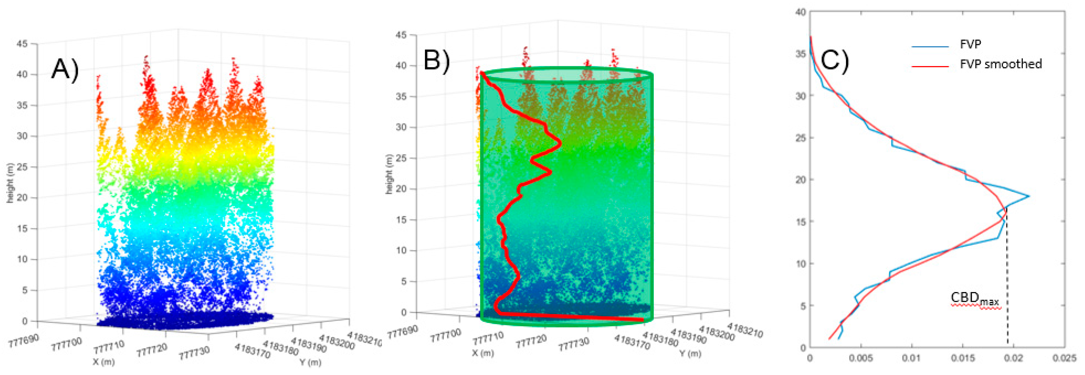
2.3. LiDAR Data and Processing

The LiDAR data used in this study were collected on November 2013 by the National Center for Airborne Laser Mapping (NCALM) using an Optech Gemini Airborne Laser Terrain Mapper (ALTM) instrument that recorded up to four returns per pulse along with their intensity. The site was flown at a mean elevation of 2200 m above sea level, with a maximum scan angle of ±14° and a nominal 50% overlap between flight lines, resulting in an average point density of approximately 20 points·m−2. The vendor provided the classified point cloud in binary LAS 1.4 format, as well as a 1-m digital elevation model (DEM) that was used to normalize the height of each return. Additionally, the DEM provided with the LiDAR data was resampled to 30 m using the average of all pixels included within the 30-m cell, and the slope and aspect were computed for each pixel. Subsequently, a set of metrics (Table 1) were derived from the height distribution of canopy returns (by applying a height threshold of 2 m) to describe the canopy structure and distribution of fuels within it. These metrics have been found to be related to different canopy fuel properties [8,13,16].
In addition to the height information, the intensity values of each LiDAR return were also used after normalizing them to a standard range [29]. This correction eliminates the effect of path length variations on the intensity of the returns, mainly caused by the rough topography of the area. Next, a set of metrics (Table 1) previously used to estimate aboveground biomass were computed [29]. Canopy cover was estimated as the ratio of the canopy energy to the total energy [14,29]. Typically, a correction factor of 2 is applied to the intensity of the ground returns to account for the differences in reflectance between canopy and ground at the wavelength of the LiDAR system [15,30]. However soil type or the presence of duff and litter affect this correction factor significantly, thus making it site-dependent. The accurate correction factor was not available for this study site and therefore it was not applied.
Additionally, the canopy reflection sum (CRS) [31] and the density-weighted canopy reflection sum (DWCRS) were computed [29], which accounts for the point density variation throughout the study site resulting from topography or scan angle.
Finally, pseudo-waveforms from the LiDAR returns were constructed for each plot [32,33] and the height of the median energy (HOME), the height/median ratio (HTRT) [34], the mean canopy height (MCH), and the quadratic mean canopy height (QMCH) were computed from the canopy height profile (CHP) [35]. Moreover, the coefficient of variation of the CHP and the area under the canopy wave were computed to describe the amount of canopy material and its vertical heterogeneity [33,36].

2.4. Landsat Data and Processing

A cloud-free orthorectified Landsat reflectance image (path/row: 043/034), acquired on 30 July 2013 was selected to estimate the canopy fuel properties. The image downloaded from the USGS Earth Explorer web site (http://earthexplorer.usgs.gov/; accessed on 21 August 2015) had been processed using the Landsat Ecosystem Disturbance Adaptive Processing System (LEDAPS) atmospheric correction (Masek et al., 2006). Radiometric calibration of the images involved (1) transformation of digital number values to at-sensor radiance based on published calibration coefficients, (2) correction to Top-Of-Atmosphere (TOA) reflectance, and (3) atmospheric correction using the 6S radiative transfer model. Further description of the methodology can be found in Masek et al. [37].
To ensure appropriate spatial alignment between the different datasets used, the Landsat image was co-registered with the LiDAR intensity image using ground control points (n = 31) and a linear transformation model, yielding an RMSE = 0.55 pixels.
In addition to the Landsat spectral bands B2-B7, the vegetation signal was enhanced by computing the Normalized Difference Vegetation Index (NDVI) [38], the Normalized Difference Infrared Index (NDII) [39], the Enhanced Vegetation Index (EVI) [40], and the Visible Atmospherically Resistant Index (VARI) [41]. The Tasseled Cap Transformation (TCT) was also calculated [42] using the coefficients derived by Baig et al. [43] and then the Tasseled Cap Angle (TCA) and Tasseled Cap Distance (TCD) [44] were computed from the TCT Greenness and Brightness components. These components are informative for describing forest structure [45,46,47,48]. TCA is responsive to vegetation cover and its gradient, and TCD is related to vegetation composition and structure [49]. Table 2 provides detailed information about the spectral metrics computed from the Landsat data.
Finally, the Landsat-based pre-fire vegetation map provided by the US Forest Service was reclassified into three vegetation types: conifers, deciduous, and mixed forest. These auxiliary layers were used in subsequent statistical analyses.

2.5. Canopy Fuel Properties Estimation from LiDAR Data

This study considered fuel load as the foliage biomass, computed using a non-linear regularized Least-Squares Support Vector Machine (LS-SVM) as implemented in the LS-SVMlab Toolbox developed by De Brabanter et al. [50] for Matlab [51]. This approach attempts to find the optimal loss function by solving a set of linear equations as an approximation for the quadratic programming problem, reducing the high computational burden associated with solving the quadratic programming problem. As usual with SVM-based techniques, non-linear modeling was achieved via the so-called “kernel trick,” using a Gaussian radial basis function (RBF) kernel. The RBF kernel is controlled by its bandwidth (h) and regularization parameter (γ) that defines the contribution of the training data error in the loss function to be minimized. These two parameters were calculated by a commonly used grid search with a five-fold cross validation.
Given the large number of metrics derived from the LiDAR data, feature selection becomes an important task, not only for processing time reasons but also for generalization performance and interpretability reasons [52]. Therefore, this study performed feature selection using three different methods including a stepwise regression approach, an evolutionary algorithm, and an expert knowledge based model. The latter method selected only two variables that potentially described the 3D structural characteristics of the canopy, namely H50 and AUCW. Further details on the feature selection and the LS-SVM approach used to estimate CFL can be found in García et al. [53].
The data from the field campaign were used to calibrate and validate the SVR model based on the features (metrics) derived from the LiDAR data. Approximately 70% of the plots were used for model calibration and 30% for independent validation.
CBD was estimated following García et al. [11]. In short, the relative canopy height profile was computed from the pseudo-waveforms generated for each plot and the previously estimated CFL was proportionally distributed through it, obtaining a canopy fuel vertical profile (FVP). The FVP was subsequently smoothed by applying a 3-m running-mean filter, and the maximum of the smoothed FVP was accepted as the CBD estimate. Figure 2 describes the method.
Finally, CC was estimated as the ratio of the number of canopy to all returns within a given area. All types of returns (first, last, and intermediate) were used in these computations.

2.6. Canopy Fuel Properties Extrapolation Using Landsat Data

Extrapolation of canopy fuel properties to the inner part of the burned area, prior to the occurrence of the megafire, was based on features derived from the Landsat image, using the LS-SVM approach. LiDAR-based canopy fuel properties were used as reference data. A random selection of >500 plots (pixels) was carried out based on the histograms of the LiDAR-derived fuel properties to ensure that full range of canopy fuel values was sampled. Approximately 60% of the sample was used for calibration and the remaining 40% was used as independent sample for validation purposes.
Feature selection was limited to a stepwise regression approach due to the unfeasibility of applying the evolutionary algorithm over this large dataset, as well as the lack of a priori knowledge of what spectral variables were related to the CFL, as these variables are not directly related to foliage biomass [53]. After applying stepwise regression using all Landsat metrics, the correlation between the selected variables was evaluated, and whenever a pair of variables showed the absolute value of the correlation coefficient >0.7 we selected the one more strongly correlated with the dependent variable.

2.7. Model Performance and Error Assessment

The performance of the SVR models was evaluated using the coefficient of determination (R2), the adjusted coefficient of determination (R2-adj), the root mean square error (RMSE), and the relative root mean square error (RRMSE). The extrapolation of the canopy fuel properties to the entire study area was based on a two-step regression approach: first, LiDAR-based estimates were obtained for each canopy fuel property, and second, a LiDAR-Landsat model was fitted to map the canopy fuel properties over the whole study area. The errors in each model, denoted by RMSELiDAR and RMSELandsat, respectively, propagated to the final estimates. Therefore, to calculate the overall error (variance) of the two-step canopy fuel estimators (i.e., σ2model) we assumed the error of the individual steps to be independent, which leads to σ2model = RMSE2LiDAR + RMSE2Landsat. A comprehensive analysis of error propagation would require considering other sources of error, such as remote sensing measurement error, sensor noise, or field measurement error. However, information on other sources of error was not available for this study, and thus these components of the error were considered negligibly small compared to the error due to modeling.
In the case of the CFL, LiDAR-based estimates were evaluated against our field-based CFL estimates. As for the CBD, we could not estimate it from the field measurements. However, several studies have found no statistically significant differences between LiDAR-derived and field-based canopy profiles [13,54,55]. Therefore, we assumed that the error of the derivation of the FVP was negligible, and thus the main source of error for CBD computation from LiDAR data resulted from the estimation of CFL. Likewise, although CC was not measured in the field, numerous previous studies have demonstrated that CC can be accurately estimated from LiDAR data. For example, Morsdorf et al. [15] reported an RMSE of 0.18 using only first returns; Hopkinson and Chasmer [14] also reported a mean error less than 0.2 in CC estimation from LiDAR data across multiple ecozones. Using these values as reference for the LiDAR-based CC estimates and an uncertainty of 18% was assumed. With regards the second step, all Landsat-based canopy fuel properties were validated against the LiDAR-based estimates.
Furthermore, the 95% confidence interval for each predicted variable was computed for each pixel using a bootstrapping pairs approach with 500 samples. Resampling techniques such as bootstrapping can be used to estimate confidence intervals as well as the variance or the standard error (square root of the variance) of the estimator and are well suited for non-parametric model approaches [56,57,58].

3. Results

3.1. Estimation of Canopy Fuel Properties from LiDAR Data

Table 3 shows the results of the SVR models developed to estimate CFL using the metrics selected by each of the feature selection algorithms. The models based on the metrics selected by stepwise regression and the genetic algorithms showed overfitting issues when applied to the independent validation datasets, with a decrease of R2 by 21% and 54% and an increase of RRMSE by 27% and 30% , respectively. The expert knowledge-based SVR model showed higher stability over the training and validation data, ensuring its applicability and generalization. This model yielded an R2 of 0.87 and 0.81, and an RRMSE of 30.4% and 33.68% for the calibration and the validation datasets, respectively. Therefore, this model was used to generate the LiDAR-based CFL map for the study area. Figure 3 shows the scatter plot of the LiDAR against the field estimates of CFL. CC and CBD were not validated against field data since these variables were not measured in the field. Nevertheless, the accuracy of the estimation for these variables from LiDAR data is sufficient to be used as reference data for the Landsat estimates, as demonstrated in other studies [14,15,59].

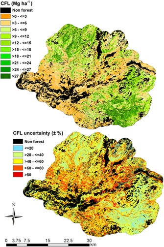
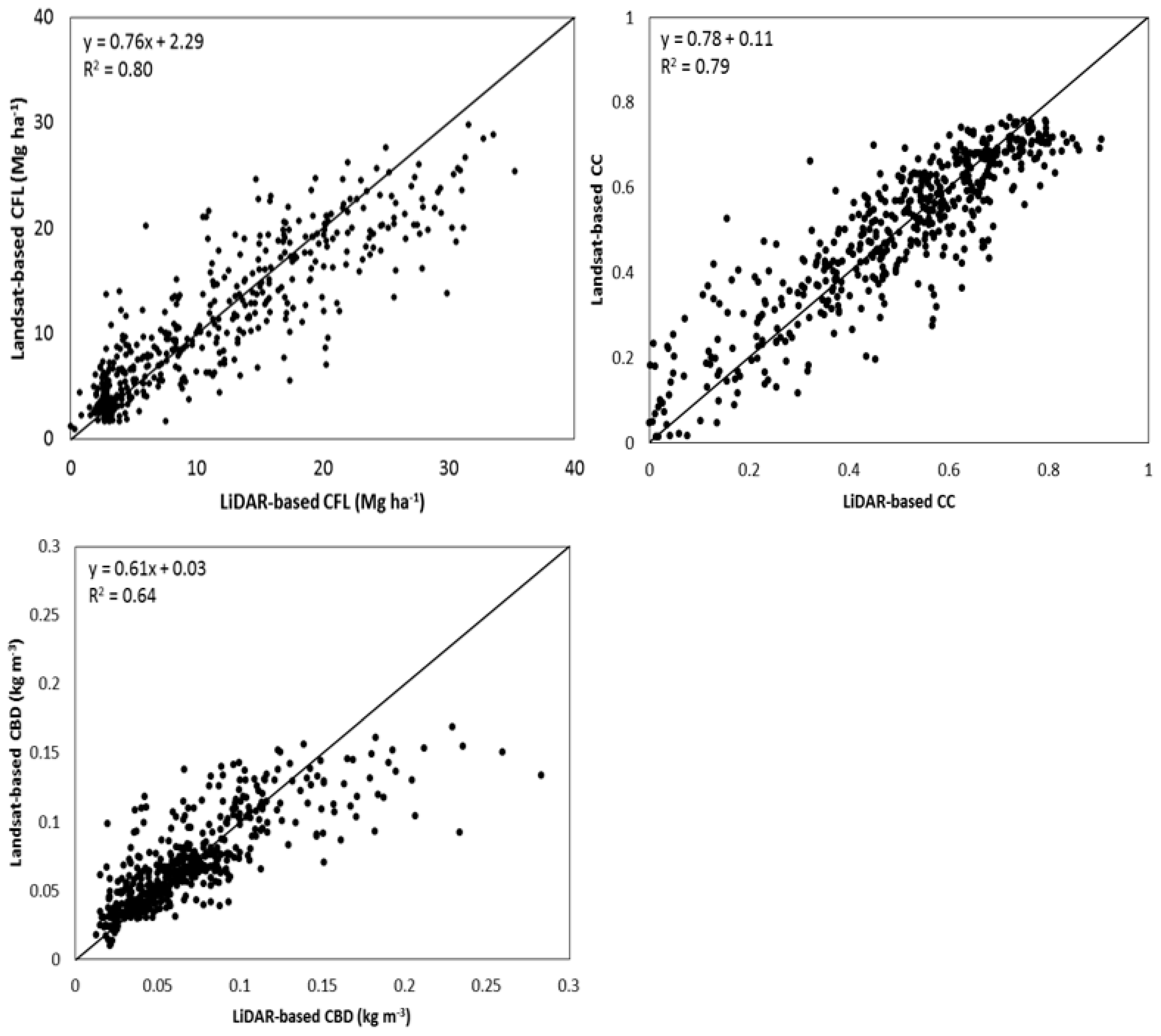
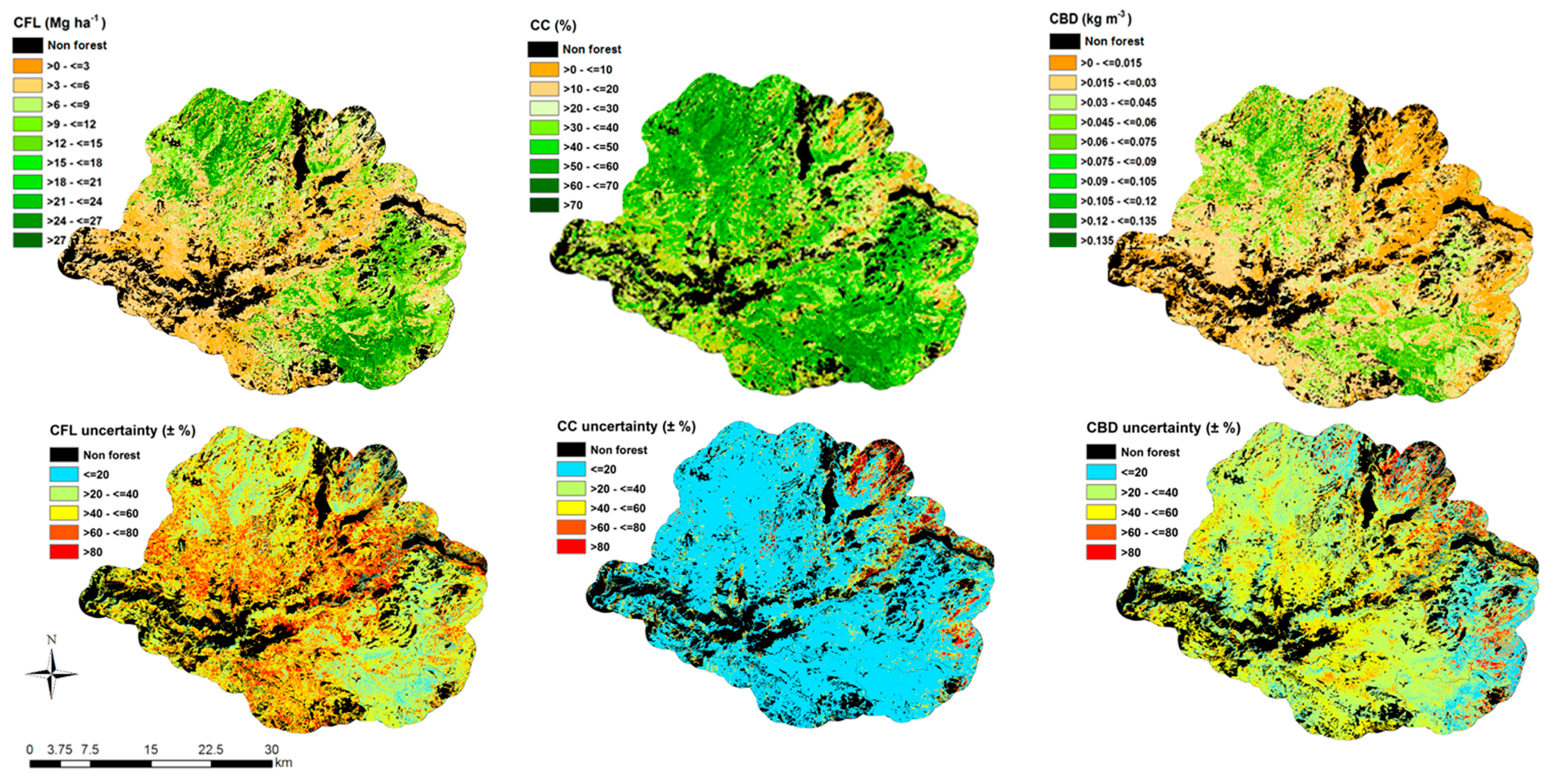
3.2. Canopy Fuel Properties Estimation from Landsat Data

The final model selected to estimate CFL included the Landsat OLI reflectance bands 2–6, the NDII, and the elevation and slope derived from the DEM. The model used to estimate CC was based only on the shortwave infrared (band 6), and the model selected to estimate CBD included the brightness and wetness components of the TCT as well as the elevation obtained from the DEM. Table 4 shows the performance of the SVR models used to extrapolate the canopy fuel properties using Landsat data. Figure 4 shows the scatter plots of the Landsat-based versus the LiDAR-based estimates, and the spatial distribution of the extrapolated canopy fuel properties is shown in Figure 5 (top row).
CFL and CC were estimated with similar accuracy and CBD was the variable estimated with the lowest accuracy. In general, low values were overestimated and high values were underestimated, especially for CBD, for which saturation of values above 0.15 kg·m−3 was observed.

3.3. Uncertainties of the Estimates

The combined uncertainty of the estimates was computed using the RMSE of the models developed at each step (Section 2.7) using the complete reference dataset, i.e., the 65 plots for the LiDAR model and the 514 pixels for the Landsat model. This resulted in an overall RRMSE of 47.64% for CFL, 26.24% for CC, and 46.73% for CBD.
Figure 5 (bottom row) shows the uncertainty of the extrapolated canopy fuel properties. Different patterns are observed among the variables. CC showed the lowest uncertainty with most of the area having values < 20%. The largest uncertainties corresponded to low CC values, some of which had estimated CC values < 10%. For CFL and CBD, similar patterns are observed, with the largest uncertainty values primarily occurring in areas of low CFL and CBD, respectively. However, larger uncertainty was observed for CFL than for CBD.

3.4. Relation between Canopy Fuel Properties and Burn Severity

This study explored the impact of the estimated canopy fuel properties on the fire effects by computing the correlation between each of them and the differenced normalized burn ratio (ΔNBR) used to estimate the burn severity [60]. To untangle the influence of the canopy fuel properties at different burned severities, the ΔNBR index was grouped into the three burn severity levels of the severity map provided by the US Forest Service.
All canopy fuel properties showed a moderate correlation with the ΔNBR index within each burn severity level except for the low severity (Table 5). The strength of the correlation increased with the level of burn severity. With regards the correlation of each variable with ΔNBR, CC had the strongest correlation, followed by CBD and CFL.

4. Discussion

4.1. Canopy Fuel Properties Estimation from LiDAR Data

The two automatic feature selection algorithms yielded models for CFL estimation that showed overfitting problems, particularly the evolutionary algorithm. Overfitted models have lower generalization capability (predictive power) and thus can produce unreliable results when applied to data that were not used for training. The model based on expert knowledge feature selection used variables that provided a description of the canopy height (H50) and the amount of canopy material within the plot (AUCW). AUCW was strongly correlated with the canopy cover (r = 0.95, p < 0.001), thus also providing information about the horizontal distribution of the vegetation. This model showed similar performance for the calibration and validation datasets and therefore, no overfitting issues.
This study did not evaluate the accuracy of our LiDAR-based CC estimates against field estimates since no measurements were collected during our field campaign. Nevertheless, LiDAR technology has been convincingly demonstrated to provide direct, physically based, and accurate canopy cover measurement, on its own [14,15]. Furthermore, validation of CC from LiDAR data is usually based on estimates from hemispherical photographs (HP), which are subject to uncertainties due to illumination conditions during photo acquisition and processing (filtering, thresholding, zenith angle range used in the CC estimation, etc.). These factors, if not carefully addressed, might produce large errors. Therefore, the reference CC data to validate Landsat OLI estimates can be derived from LiDAR over much larger areas than using field methods, thus allowing the benefits of large samples for modeling.
It was assumed that the error of the LiDAR-based CBD estimates mainly resulted from the CFL model error. This assumption is supported by other studies showing no statistically significant differences between canopy profiles derived from LiDAR data and those from the field [54,55]. Although the canopy profiles were derived from pseudo-waveforms, the very high point density of LiDAR data (20 points m−2) guaranteed having more than the minimum number of returns necessary to derive acceptable pseudo-waveforms [33]. Furthermore, the LiDAR-based canopy profiles provided a more realistic representation of the canopy fuel distribution than the one that would be obtained by using limited field measurements and describing the shape of the crown using a cylindrical or conical shape as commonly done.

4.2. Canopy Fuel Properties Estimation from Landsat Data

Although passive sensors are less sensitive to structure than active sensors, it is possible to relate the spectral information to structural characteristics of the forest [61]. Thus, the correlation between the spectral information contained in the Landsat bands and structural properties of the canopy, including biomass and CC, have been demonstrated over different forest types [48,62]. The models used to estimate the canopy fuel properties also included the NDII as well as the brightness and wetness components of the TCT. Spectral indices including the shortwave infrared have been proved to have higher sensitivity to high LAI values [63,64], whereas TCT components have shown their suitability to infer information on stand age and forest structure [45,46,48], particularly for mature and old growth stands.
The three canopy variables were estimated accurately, with R2 ranging from 0.66 (CBD) to 0.85 (CFL) and RRMSE ranging from 18.88% (CC) to 36.71% (CBD) for the calibration datasets. CBD was the variable for which the model performed the worst, as was expected given the limited capability of multispectral sensors to represent the vertical distribution of the canopy fuels. However, the CBD estimates showed better accuracy than those obtained in other studies using passive multispectral data. For instance, Falkowski et al. [24] reported R2 from 0.06 to 0.47 and RMSE from 0.0485 to 0.052 kg·m−3 using ASTER data. A higher R2 of 0.60 was reported by Erdody and Moskal [65] using aerial imagery. Based on Landsat data, R2 between 0.33 and 0.55 has been reported by Palaiologou et al. [25] and Pierce et al. [66], respectively. With regards to CFL, this study was also able to obtain better accuracy than previously reported. Thus, Erdody and Moskal [65] obtained R2 = 0.67, although the relatively poor spectral information of their data (green, red and near infrared) and the fact that no ancillary data was used has to be born in mind.
Out of the three canopy variables estimated, CC is the one that is usually estimated with the highest accuracy using passive data. R2 of 0.68 and 0.67 were reported for Landsat data by Palaiologou et al. [25] and Pierce et al. [66], respectively. Better results were reported for ASTER by Falkowski et al. [24], with R2 from 0.08 to 0.77 and RMSE from 16.56% to 32.35%.
The higher accuracy for estimating canopy fuel properties in our results could stem from the use of different modeling approaches, differences in the spatial and spectral information of the data used, as well as the different reference data used to validate the results. Whereas the published studies discussed above were generally based on multiple linear regressions, this study used an SVR, a non-parametric approach that can better capture complex non-linear relationships between the dependent and the explanatory variables [59]. In addition, spectral indices were used based on bands sensitive to the water content, which are more sensitive to high LAI and biomass values, thus reducing the saturation effect. Pierce et al. [66] used a non-parametric random forest approach with similar variables to the ones we used here. The higher uncertainties of their estimates could result from the difference between the plot size (500 m2) and the area covered by a Landsat pixel (900 m2), as well as the different type of reference data used to validate the results. They used hemispherical photographs, while for this study LiDAR-based estimates were used.

4.3. Uncertainty Analyses

The final errors of our estimates, after the error propagation of our two-step approach, were RMSECBD = 0.033 kg·m−3 (RRMSECBD = 46.73%); RMSECFL = 4.82 Mg·ha−1 (RRMSECFL = 47.64%); RMSECC = 0.20 (RRMSECC = 26.24%). Despite the high combined high error obtained for CFL and CBD, the accuracy of these results is better than those reported by other studies. This study did not account for possible errors in the allometric equations and thus made an implicit assumption that the field estimates are ground truth. This assumption is common to other studies, but more efforts should be devoted in the future to account for this source of error in order to fully characterize the uncertainty of the canopy fuel products.
This study also assumed that the errors in CBD estimates resulted only from the estimation of CFL. This assumption is supported by other studies showing no statistically significant differences between field-based and LiDAR-based canopy profiles and the very high point density used, which allowed a detailed description of the vertical distribution of the fuels from the derived pseudo-waveforms. Moreover, validation of this variable is challenging due to the difficulty in measuring CBD in the field, with no standardized field methods and based on numerous assumptions of crown shape and distributions of the fuel load through the crown. In the case of CC, accuracy values from the literature were used for the LiDAR-based estimates, which were based on the comparison of LiDAR estimates with HP. Although HP is a well-established method to indirectly measure CC, illumination conditions during the acquisition and the processing of the photographs, can significantly affect the results. In addition, uncertainties about the area covered by the photographs remain. Therefore, further efforts are needed to fully characterize the accuracy of the canopy fuel products, which in some cases would need refinement or development of new field methods. Terrestrial LiDAR systems have a proven capability for characterizing canopy fuels [10,67], offering great potential as reference data for airborne and satellite product validation.
A bootstrapping pairs approach was used to derive the uncertainty for each estimated fuel property at the pixel level. The larger uncertainties were observed for lower canopy fuel properties values, probably due to the higher within pixel heterogeneity of those pixels as a result of canopy gaps and soil effects on the spectral signal. Canopy cover was the least uncertainty variable since passive sensors can provide accurate characterization of the horizontal distribution of the canopy material. CBD showed a clear saturation effect over 0.15 kg·m−3 due to the lower sensitivity of passive sensors to the three dimensional arrangement of canopy elements, particularly for dense canopies.

4.4. Relation between Canopy Fuel Properties and Burn Severity

The three canopy fuel properties showed moderate correlation with the ΔNBR index at moderate and high burn severity levels. At low burn severity levels, CC and CBD did not correlate with burn severity and CFL presented a moderately negative correlation. This lack of correlation was expected since tree crowns are not affected at low burn severity areas. CC was the variable with the strongest correlation with ΔNBR, followed by CBD. Graham et al. [68] indicated the importance of reducing the amount of fuel as well as its vertical and horizontal continuity for reducing fire severity. The results support this statement, although they suggest that the horizontal distribution of the canopy fuels is the most important variable determining burn severity. Nevertheless, the limited capability of Landsat-based severity measures to capture actual damage caused by fire to the understory and midstory vegetation in low and moderate severity areas [69] could bias the conclusions of this study, since CC is measured more accurately by passive sensors.
The weakest correlation found for CFL can be explained by the fact that burn severity is a measure of the relative fire damage, which can be the same for areas with different fuel loads. Our results provide insights into the effect of canopy fuel properties on burn severity. However, other factors affecting fire behavior such as fuel moisture or weather conditions should be considered in future studies in order to reach more definitive conclusions. Furthermore, this study only considered canopy fuel properties whereas the ΔNBR will also be affected by understory vegetation, particularly over more open areas.

5. Conclusions

This research demonstrated how LiDAR-based canopy fuel properties can be extrapolated to larger regions using Landsat data. The method, which relies on a two-step approach, exploits the ability of LiDAR data to estimate canopy fuel properties with high accuracy (step 1) and the larger spatial coverage and higher acquisition frequency of satellite data to accurately extrapolate the canopy fuel properties over larger areas (step 2). In addition, the uncertainty of the estimates was provided at the pixel level.
The proposed method to characterize forest canopy fuels is particularly relevant in two ways for the Landscape Fire and Resource Management Planning Tools (LANDFIRE) program, which provides canopy fuel properties at 30 m resolution based on Landsat data. First, it proves how airborne LiDAR data can be integrated with Landsat data to extrapolate accurate LiDAR-based canopy fuel properties to provide improved continuous spatial information on canopy fuel properties over large regions. Second, this extrapolation is based on Landsat data, which is the basic data source used by the LANDFIRE program. Thus, airborne LiDAR data samples collected for instance by local agencies or NASA’s G-LiHT could be used along with the Landsat archive data to characterize canopy fuels regionally.
These results show improved performance against other studies based on Landsat data alone. This is of considerable importance since the results of fire behavior and fire effect models depend on the quality of the fuel products used as inputs. Moreover, improved, spatially explicit information on canopy fuels is critical to making fire management and mitigation more effective and improving ecosystem resiliency.
This paper also investigated the relation between burn severity and three important canopy fuel properties, suggesting that the horizontal distribution of the canopy fuels had a higher effect on burn severity than its vertical distribution.

Acknowledgments

This research was carried out within the ambit of the project “Multi-sensor remote sensing study of California’s Rim Fire to inform post-fire ecosystem restoration and effective prevention of future catastrophic wildfires” funded by USDA Forest Service, as the main sponsor, and the University of California Davis under Cost Share Agreement 10-IA-11130400-009. Mariano Garcia is supported by the Marie Curie International Outgoing Fellowship within the Seventh European Community Framework Programme (ForeStMap-3D Forest Structure Monitoring and Mapping, Project Reference: 629376). The contents on this paper reflect only the authors’ views and not the views of the European Commission. This study was partially funded by the Natural Environment Research Council’s support for the National Centre for Earth Observation. H. Balzter was supported by the Royal Society Wolfson Research Merit Award, 2011/R3 and the NERC National Centre for Earth Observation. The research was carried out at the Jet Propulsion Laboratory, California Institute of Technology, under a contract with the National Aeronautics and Space Administration. The authors greatly appreciate the help of Mitzi Thornley and the Science Division Yosemite National Park for the permission to conduct research in Yosemite National Park (YOSE-00653/YOSE-2014-SCI-0124). Comments from Dr. Riaño are highly appreciated.

Author Contributions

M.G., S.S., S.U., A.K., and H.B. designed the research and drafted the manuscript. M.G., A.K., S.L.U., A.C., and C.R. designed the field work. M.G. processed and analyzed the data. All authors read and approved the final manuscript.

Conflicts of Interest

The authors declare no conflict of interest. Airborne LiDAR and field data collection was founded by USDA Forest Service, as the main sponsor, and the University of California Davis under Cost Share Agreement 10-IA-11130400-009.

References

  1. Keane, R.E.; Burgan, R.; van Wagtendonk, J. Mapping wildland fuels for fire management across multiple scales: Integrating remote sensing, GIS, and biophysical modeling. Int. J. Wildland Fire 2001, 10, 301–319. [Google Scholar] [CrossRef]
  2. Stephens, S.; Agee, J.K.; Fulé, P.; North, M.; Romme, W.; Swetnam, T.; Turner, M.G. Managing Forests and Fire in Changing Climates. Science 2013, 342, 41–42. [Google Scholar] [CrossRef] [PubMed]
  3. Williams, J.; Albright, D.; Hoffmann, A.A.; Eritsov, A.; Moore, P.F.; Mendes de Morais, J.C.; Leonard, M.; Miguel-Ayanz, J.S.; Xanthopoulos, G.; van Lierop, P. Findings and Implications from a Coarse-Scale Global Assessment of Recent Selected Mega-Fires. In Proceedings of the 5th International Wildland Fire Conference, Sun City, South Africa, 9–13 May 2011. [Google Scholar]
  4. Attiwill, P.; Binkley, D. Exploring the mega-fire reality: A “Forest Ecology and Management” conference. For. Ecol. Manag. 2013, 294, 1–3. [Google Scholar] [CrossRef]
  5. Scott, J.H.; Reinhardt, E.D. Assessing Crown Fire Potential by Linking Models of Surface and Crown Fire Behavior; Research Paper RMRS-RP-29; USDA Forest Service, Rocky Mountain Research Station: Fort Collins, CO, USA, 2001. [Google Scholar]
  6. Cruz, M.G.; Alexander, M.E.; Wakimoto, R.H. Assessing canopy fuel stratum characteristics in crown fire prone fuel types of western North America. Int. J. Wildland Fire 2003, 12, 39–50. [Google Scholar] [CrossRef]
  7. Keane, R.E.; Reinhardt, E.D.; Scott, J.; Gray, K.; Reardon, J. Estimating forest canopy bulk density using six indirect methods. Can. J. For. Res. 2005, 35, 724–739. [Google Scholar] [CrossRef]
  8. Riaño, D.; Meier, E.; Allgöwer, B.; Chuvieco, E.; Ustin, S.L. Modeling airborne laser scanning data for the spatial generation of critical forest parameters in fire behavior modeling. Remote Sens. Environ. 2003, 86, 177–186. [Google Scholar] [CrossRef]
  9. Van Wagner, C.E. Conditions for the start and spread of crown fire. Can. J. For. Res. 1977, 7, 23–34. [Google Scholar] [CrossRef]
  10. García, M.; Danson, F.M.; Riano, D.; Chuvieco, E.; Ramirez, F.A.; Bandugula, V. Terrestrial laser scanning to estimate plot-level forest canopy fuel properties. Int. J. Appl. Earth Obs. Geoinform. 2011, 13, 636–645. [Google Scholar] [CrossRef]
  11. García, M.; Popescu, S.; Riaño, D.; Zhao, K.; Neuenschwander, A.; Agca, M.; Chuvieco, E. Characterization of canopy fuels using ICESat/GLAS data. Remote Sens. Environ. 2012, 123, 81–89. [Google Scholar] [CrossRef]
  12. Riano, D.; Chuvieco, E.; Condés, S.; González-Matesanz, J.; Ustin, S.L. Generation of crown bulk density for Pinus sylvestris L. from lidar. Remote Sens. Environ. 2004, 92, 345–352. [Google Scholar] [CrossRef]
  13. Skowronski, N.S.; Clark, K.L.; Duveneck, M.; Hom, J. Three-dimensional canopy fuel loading predicted using upward and downward sensing LiDAR systems. Remote Sens. Environ. 2011, 115, 703–714. [Google Scholar] [CrossRef]
  14. Hopkinson, C.; Chasmer, L. Testing LiDAR models of fractional cover across multiple forest ecozones. Remote Sens. Environ. 2009, 113, 275–288. [Google Scholar] [CrossRef]
  15. Morsdorf, F.; Kötz, B.; Meier, E.; Itten, K.I.; Allgöwer, B. Estimation of LAI and fractional cover from small footprint airborne laser scanning data based on gap fraction. Remote Sens. Environ. 2006, 104, 50–61. [Google Scholar] [CrossRef]
  16. Andersen, H.E.; McGaughey, R.J.; Reutebuch, S.E. Estimating forest canopy fuel parameters using LIDAR data. Remote Sens. Environ. 2005, 94, 441–449. [Google Scholar] [CrossRef]
  17. Hall, S.A.; Burke, I.C.; Box, D.O.; Kaufmann, M.R.; Stoker, J.M. Estimating stand structure using discrete-return lidar: An example from low density, fire prone ponderosa pine forests. For. Ecol. Manag. 2005, 208, 189–209. [Google Scholar] [CrossRef]
  18. Gajardo, J.; García, M.; Riaño, D. Applications of Airborne Laser Scanning in forest fuel assessment and fire prevention. In Forestry Applications of Airborne Laser Scanning Concepts and Case Studies; Maltamo, M., Naesset, E., Vauhkonen, J., Eds.; Springer: Dordrecht, The Netherlands, 2014. [Google Scholar]
  19. Gwenzi, D.; Lefsky, M.A.; Suchdeo, V.P.; Harding, D.J. Prospects of the ICESat-2 laser altimetry mission for savanna ecosystem structural studies based on airborne simulation data. ISPRS J. Photogramm. Remote Sens. 2016, 118, 68–82. [Google Scholar] [CrossRef]
  20. Dubayah, R.; Goetz, S.J.; Blair, J.B.; Fatoyinbo, T.E.; Hansen, M.; Healey, S.P.; Hofton, M.A.; Hurtt, G.C.; Kellner, J.; Luthcke, S.B.; et al. The Global Ecosystem Dynamics Investigation (GEDI) Lidar. AGU Fall Meet. Abstr. 2014, 1, 7. Available online: https://agu.confex.com/agu/fm14/meetingapp.cgi/Paper/26237 (accessed on 10 January 2017).
  21. Maselli, F.; Chiesi, M.; Montaghi, A.; Pranzini, E. Use of ETM+ images to extend stem volume estimates obtained from LiDAR data. ISPRS J. Photogramm. Remote Sens. 2011, 66, 662–671. [Google Scholar] [CrossRef]
  22. Saatchi, S.S.; Harris, N.L.; Brown, S.; Lefsky, M.; Mitchard, E.T.; Salas, W.; Zutta, B.R.; Buermann, W.; Lewis, S.L.; Hagen, S.; et al. Benchmark map of forest carbon stocks in tropical regions across three continents. Proc. Natl. Acad. Sci. USA 2011, 108, 9899–9904. [Google Scholar] [CrossRef] [PubMed]
  23. Wulder, M.A.; White, J.C.; Nelson, R.F.; Næsset, E.; Ørka, H.O.; Coops, N.C.; Hilker, T.; Bater, C.W.; Gobakken, T. Lidar sampling for large-area forest characterization: A review. Remote Sens. Environ. 2012, 121, 196–209. [Google Scholar] [CrossRef]
  24. Falkowski, M.J.; Gessler, P.E.; Morgan, P.; Hudak, A.T.; Smith, A.M. Characterizing and mapping forest fire fuels using ASTER imagery and gradient modeling. For. Ecol. Manag. 2005, 217, 129–146. [Google Scholar] [CrossRef]
  25. Palaiologou, P.; Kalabokidis, K.; Kyriakidis, P. Forest mapping by geoinformatics for landscape fire behaviour modelling in coastal forests, Greece. Int. J. Remote Sens. 2013, 34, 4466–4490. [Google Scholar] [CrossRef]
  26. Casas, Á.; García, M.; Siegel, R.B.; Koltunov, A.; Ramírez, C.; Ustin, S. Burned forest characterization at single-tree level with airborne laser scanning for assessing wildlife habitat. Remote Sens. Environ. 2016, 175, 231–241. [Google Scholar] [CrossRef]
  27. Wang, Y.F. National Biomass Estimator Library; Forest Management Service Center: Fort Collins, CO, USA, 2014. [Google Scholar]
  28. Keyser, C.E.; Dixon, G.E. Western Sierra Nevada (WS) Variant Overview Forest Vegetation Simulator; Forest Management Service Center: Fort Collins, CO, USA, 2012; p. 58. [Google Scholar]
  29. García, M.; Riaño, D.; Chuvieco, E.; Danson, F.M. Estimating biomass carbon stocks for a Mediterranean forest in Spain using height and intensity LiDAR data. Remote Sens. Environ. 2010, 114, 816–830. [Google Scholar] [CrossRef]
  30. Lefsky, M.A.; Harding, D.; Cohen, W.B.; Parker, G.; Shugart, H.H. Surface Lidar Remote Sensing of Basal Area and Biomass in Deciduous Forests of Eastern Maryland, USA. Remote Sens. Environ. 1999, 67, 83–98. [Google Scholar] [CrossRef]
  31. Means, J.E.; Acker, S.A.; Harding, D.J.; Blair, J.B.; Lefsky, M.A.; Cohen, W.B.; Harmon, M.E.; McKee, W.A. Use of Large-Footprint Scanning Airborne Lidar To Estimate Forest Stand Characteristics in the Western Cascades of Oregon. Remote Sens. Environ. 1999, 67, 298–308. [Google Scholar] [CrossRef]
  32. Blair, J.B.; Hofton, M.A. Modeling laser altimeter return waveforms over complex vegetation using high-resolution elevation data. Geophys. Res. Lett. 1999, 26, 2509–2512. [Google Scholar] [CrossRef]
  33. Muss, J.D.; Mladenoff, D.J.; Townsend, P.A. A pseudo-waveform technique to assess forest structure using discrete lidar data. Remote Sens. Environ. 2011, 115, 824–835. [Google Scholar] [CrossRef]
  34. Drake, J.B.; Dubayah, R.O.; Knox, R.G.; Clark, D.B.; Blair, J.B. Sensitivity of large-footprint lidar to canopy structure and biomass in a neotropical rainforest. Remote Sens. Environ. 2002, 81, 378–392. [Google Scholar] [CrossRef]
  35. Lefsky, M.A.; Cohen, W.B.; Acker, S.A.; Parker, G.G.; Spies, T.A.; Harding, D. Lidar Remote Sensing of the Canopy Structure and Biophysical Properties of Douglas-Fir Western Hemlock Forests. Remote Sens. Environ. 1999, 70, 339–361. [Google Scholar] [CrossRef]
  36. Bouvier, M.; Durrieu, S.; Fournier, R.A.; Renaud, J.P. Generalizing predictive models of forest inventory attributes using an area-based approach with airborne LiDAR data. Remote Sens. Environ. 2015, 156, 322–334. [Google Scholar] [CrossRef]
  37. Masek, J.G.; Vermote, E.F.; Saleous, N.E.; Wolfe, R.; Hall, F.G.; Huemmrich, K.F.; Gao, F.; Kutler, J.; Lim, T.K. A Landsat surface reflectance dataset for North America, 1990–2000. IEEE Geosci. Remote Sens. Lett. 2006, 3, 68–72. [Google Scholar] [CrossRef]
  38. Tucker, C.J. Red and photographic infrared linear combinations for monitoring vegetation. Remote Sens. Environ. 1979, 8, 127–150. [Google Scholar] [CrossRef]
  39. Hunt, R.E.; Rock, B.N. Detection of changes in leaf water content using near- and middle-infrared reflectances. Remote Sens. Environ. 1989, 30, 43–54. [Google Scholar]
  40. Huete, A.; Didan, K.; Miura, T.; Rodriguez, E.P.; Gao, X.; Ferreira, L.G. Overview of the radiometric and biophysical performance of the MODIS vegetation indices. Remote Sens. Environ. 2002, 83, 195–213. [Google Scholar] [CrossRef]
  41. Gitelson, A.A.; Kaufman, Y.J.; Stark, R.; Rundquist, D. Novel algorithms for remote estimation of vegetation fraction. Remote Sens. Environ. 2002, 80, 76–87. [Google Scholar] [CrossRef]
  42. Kauth, R.J.; Thomas, G.S. The tasseled cap—A graphic description of the spectral temporal development of agricultural crops as seen by Landsat. Proceding of the Symposium on Machine Processing of Remotely Sensed Data, West Lafayette, IN, USA, 29 June–1 July 1976; pp. 47–51. [Google Scholar]
  43. Baig, M.H.A.; Zhang, L.; Shuai, T.; Tong, Q. Derivation of a tasselled cap transformation based on Landsat 8 at-satellite reflectance. Remote Sens. Lett. 2014, 5, 423–431. [Google Scholar] [CrossRef]
  44. Powell, S.L.; Cohen, W.B.; Healey, S.P.; Kennedy, R.E.; Moisen, G.G.; Pierce, K.B.; Ohmann, J.L. Quantification of live aboveground forest biomass dynamics with Landsat time-series and field inventory data: A comparison of empirical modeling approaches. Remote Sens. Environ. 2010, 114, 1053–1068. [Google Scholar] [CrossRef]
  45. Cohen, W.B.; Spies, T.A.; Fiorella, M. Estimating the age and structure of forests in a multi-ownership landscape of western Oregon, U.S.A. Int. J. Remote Sens. 1995, 16, 721–746. [Google Scholar] [CrossRef]
  46. Hansen, M.J.; Franklin, S.E.; Woudsma, C.; Peterson, M. Forest Structure Classification in the North Columbia Mountains Using the Landsat TM Tasseled Cap Wetness Component. Can. J. Remote Sens. 2001, 27, 20–32. [Google Scholar] [CrossRef]
  47. Pascual, C.; Garcia-Abril, A.; Cohen, W.B.; Martin-Fernandez, S. Relationship between LiDAR-derived forest canopy height and Landsat images. Int. J. Remote Sens. 2010, 31, 1261–1280. [Google Scholar] [CrossRef]
  48. Wulder, M.A.; Skakun, R.S.; Kurz, W.A.; White, J.C. Estimating time since forest harvest using segmented Landsat ETM+ imagery. Remote Sens. Environ. 2004, 93, 179–187. [Google Scholar] [CrossRef]
  49. Pflugmacher, D.; Cohen, W.B.; Kennedy, R.E.; Yang, Z. Using Landsat-derived disturbance and recovery history and lidar to map forest biomass dynamics. Remote Sens. Environ. 2014, 151, 124–137. [Google Scholar] [CrossRef]
  50. De Brabanter, K.; Karsmakers, P.; Ojeda, F.; Alzate, C.; de Brabanter, J.; Pelckmans, K.; de Moor, B.; Vandewalle, J.; Suykens, J.A.K. LS-SVMlab Toolbox User’s Guide Version 1.8; Katholieke Universiteit Leuven: Leuven, Belgium, 2011; Available online: http://www.esat.kuleuven.be/sista/lssvmlab/downloads/tutorialv1_8.pdf (accessed on 10 March 2017).
  51. Matlab. The Mathworks Inc.: Natick, MA, USA, 2010. Available online: https://uk.mathworks.com/products/matlab.html (accessed on 10 March 2017).
  52. Weston, J.; Mukherjee, S.; Chapelle, O.; Pontil, M.; Poggio, T.; Vapnik, V. Feature selection for SVMS. Adv. Neural Inf. Process. Syst. 2000, 13, 668–674. [Google Scholar]
  53. Garcia, M.; Saatchi, S.; Casas, A.; Koltunov, A.; Ustin, S.; Ramirez, C.; Garcia-Gutierrez, J.; Balzter, H. Quantifying biomass consumption and carbon release from the California Rim fire by integrating airborne LiDAR and Landsat OLI data. J. Geophys. Res. Biogeosci. 2017, 122, 340–353. [Google Scholar] [CrossRef] [PubMed]
  54. Fieber, K.D.; Davenport, I.J.; Tanase, M.A.; Ferryman, J.M.; Gurney, R.J.; Becerra, V.M.; Walker, J.P.; Hacker, J.M. Validation of Canopy Height Profile methodology for small-footprint full-waveform airborne LiDAR data in a discontinuous canopy environment. ISPRS J. Photogramm. Remote Sens. 2015, 104, 144–157. [Google Scholar] [CrossRef]
  55. Harding, D.J.; Lefsky, M.A.; Parker, G.G.; Blair, J.B. Laser altimeter canopy height profiles: Methods and validation for closed-canopy, broadleaf forests. Remote Sens. Environ. 2001, 76, 283–297. [Google Scholar] [CrossRef]
  56. McRoberts, R.E.; Magnussen, S.; Tomppo, E.O.; Chirici, G. Parametric, bootstrap, and jackknife variance estimators for the k-Nearest Neighbors technique with illustrations using forest inventory and satellite image data. Remote Sens. Environ. 2011, 115, 3165–3174. [Google Scholar] [CrossRef]
  57. Montesano, P.M.; Nelson, R.F.; Dubayah, R.O.; Sun, G.; Cook, B.D.; Ranson, K.J.R.; Næsset, E.; Kharuk, V. The uncertainty of biomass estimates from LiDAR and SAR across a boreal forest structure gradient. Remote Sens. Environ. 2014, 154, 398–407. [Google Scholar] [CrossRef]
  58. Sun, G.; Ranson, K.J.; Guo, Z.; Zhang, Z. Forest biomass mapping from lidar and radar synergies. Remote Sens. Environ. 2011, 115, 2906–2916. [Google Scholar] [CrossRef]
  59. Zhao, K.; Popescu, S.; Meng, X.; Pang, Y.; Agca, M. Characterizing forest canopy structure with lidar composite metrics and machine learning. Remote Sens. Environ. 2011, 115, 1978–1996. [Google Scholar] [CrossRef]
  60. Cocke, A.E.; Fulé, P.Z.; Crouse, J.E. Comparison of burn severity assessments using Differenced Normalized Burn Ratio and ground data. Int. J. Wildland Fire 2005, 14, 189–198. [Google Scholar] [CrossRef]
  61. Huesca, M.; Garcia, M.; Roth, K.L.; Casas, A.; Ustin, S.L. Canopy structural attributes derived from AVIRIS imaging spectroscopy data in a mixed broadleaf/conifer forest. Remote Sens. Environ. 2016, 182, 208–226. [Google Scholar] [CrossRef]
  62. Jakubauskas, M.E.; Price, K.P. Empirical relationships between structural and spectral factors of Yellowstone Lodgepole Pine forests. Photogramm. Eng. Remote Sens. 1997, 63, 1375–1381. [Google Scholar]
  63. Lu, D.; Mausel, P.; Brondızio, E.; Moran, E. Relationships between forest stand parameters and Landsat TM spectral responses in the Brazilian Amazon Basin. For. Ecol. Manag. 2004, 198, 149–167. [Google Scholar] [CrossRef]
  64. Roberts, D.A.; Ustin, S.L.; Ogunjemiyo, S.; Greenberg, J.; Dobrowski, S.Z.; Chen, J.; Hinckley, T.M. Spectral and Structural Measures of Northwest Forest Vegetation at Leaf to Landscape Scales. Ecosystems 2004, 7, 545–562. [Google Scholar] [CrossRef]
  65. Erdody, T.L.; Moskal, L.M. Fusion of LiDAR and imagery for estimating forest canopy fuels. Remote Sens. Environ. 2010, 114, 725–737. [Google Scholar] [CrossRef]
  66. Pierce, A.D.; Farris, C.A.; Taylor, A.H. Use of random forests for modeling and mapping forest canopy fuels for fire behavior analysis in Lassen Volcanic National Park, California, USA. For. Ecol. Manag. 2012, 279, 77–89. [Google Scholar] [CrossRef]
  67. Loudermilk, E.L.; Hiers, J.K.; O’Brien, J.J.; Mitchell, R.J.; Singhania, A.; Fernandez, J.C.; Cropper, W.P.; Slatton, K.C. Ground-based LIDAR: A novel approach to quantify fine-scale fuelbed characteristics. Int. J. Wildland Fire 2009, 18, 676–685. [Google Scholar] [CrossRef]
  68. Graham, R.T.; McCaffrey, S.; Jain, T.B. Science Basis for Changing Forest Structure to Modify Wildfire Behavior and Severity; Technical Report; USDA Forest Service, Rocky Mountain Research Station: Washington, DC, USA, 2004. [Google Scholar]
  69. Miller, J.D.; Quayle, B. Calibration and validation of inmediate post-fire satellite-derived data to three severity metrics. Fire Ecol. 2015, 11, 12–30. [Google Scholar] [CrossRef]
Figure 1. Study area comprising the footprint of the Rim fire in the Sierra Nevada Mountains, CA.
Remotesensing 09 00394 g001
Figure 2. Schematic representation of the method used to estimate canopy bulk density (CBD) from the airborne LiDAR data. (A) LiDAR point cloud of a 0.09 ha plot; (B) Vertical distribution of canopy elements derived from the LiDAR pseudo-waveform; (C) Derivation of the fuel vertical profile from LiDAR data and estimation of CBD using the maximum of the smoothed FVP.
Remotesensing 09 00394 g002
Figure 3. Scatter plot of LiDAR-based versus field-based CFL estimates. The solid line represents the 1:1 line.
Remotesensing 09 00394 g003
Figure 4. Scatter plots of LiDAR-based versus Landsat OLI canopy fuel properties. Left, canopy fuel load; center, canopy cover; right, canopy bulk density. The solid line represents the 1:1 line.
Remotesensing 09 00394 g004
Figure 5. Spatial distribution of the Landsat-based extrapolated canopy fuel properties and the associated uncertainties. Left, canopy fuel load; center, canopy cover; right, canopy bulk density.
Remotesensing 09 00394 g005
Table 1. LiDAR metrics derived from the height and intensity distributions of the returns.
HeightLabelIntensityLabelPseudo-WaveformLabel
25th PercentileH2525th Percentile intensityI25Height of Median EnergyHOME
50th PercentileH5050th Percentile intensityI50Height to median ratioHTRT
75th PercentileH7575th Percentile intensityI75Mean Canopy HeightMCH
90th PercentileH9090th Percentile intensityI90Quadratic Mean Canopy HeightQMCH
99th PercentileH9999th Percentile intensityI99Coefficient of Variation of the CHPCVCHP
Mean heightMean_hMean intensityMean_iArea Under Canopy WaveformAUCW
Standard deviationStd_hStandard deviation intensityStd_i
Canopy depthCD_hCoefficient of VariationCV_i
KurtosisKurt_hRange of intensitiesRange_i
SkewnessSkew_hSkewnessSkew_i
Coefficient of VariationCV_hKurtosisKurt_i
99th–50th percentileH99-H50Canopy CoverCC_i
99th–25th percentileH99-H25% of intensity accumulated at H25%Int_H25
90th–50th percentileH90-H50% of intensity accumulated at H50%Int_H50
90th–25th percentileH90-H25% of intensity accumulated at H75%Int_H75
Canopy CoverCC_h% of intensity accumulated at H90%Int_H90
% of intensity accumulated at H99%Int_H99
Canopy Reflection SumCRS
Density Weighted Canopy Reflection SumDWCRS
Table 2. Spectral indices and band transformations applied to the Landsat OLI imagery.
Spectral IndexFormulationParameters
NDVI = ( ρ N I R ρ R ρ N I R + ρ R ) ρR: Reflectance in the red spectral region
ρNIR: Reflectance in the near infrared spectral region
ρSWIR: Reflectance in the shortwave infrared spectral region (either 1 or 2, which are in the 1.7–1.9 µm or 2.1–2.5 µm region, respectively
G: Gain factor. Value = 2.5
C1 & C2: Coefficients of the aerosol resistance term. Values = 6 & 7.5, respectively
L: Soil-adjustment factor. Value = 1
ρB: Reflectance in the blue spectral region
ρG: Reflectance in the green spectral region
TCG: Tasseled Cap Greenness
TCB: Tasseled Cap Brightness
NDII = ( ρ N I R ρ S W I R ρ N I R + ρ S W I R )
EVI = G ( ρ N I R ρ R ρ N I R + C 1 × ρ R C 2 × ρ B + L )
VARI = ( ρ G ρ R ρ G + ρ R ρ B )
(TCA) = arctan ( T C G T C B )
(TCD) = T C B 2 + T C G 2
ΔNBR ** N B R p r e f i r e N B R p o s t f i r e
where NBR* is computed as: ( ρ N I R ρ S W I R 2 ρ N I R + ρ S W I R 2 )
* NBR: Normalized Burn Ratio; ** ΔNBR: Differenced Normalized Burn Ratio.
Table 3. Features selected and SVR-model accuracies obtained by each feature selection algorithm to estimate canopy fuel load (CFL). The first line corresponds to the calibration dataset, the second line corresponds to the validation dataset, and the third line (in bold) correspond the accuracy for the combined datasets.
Feature SelectionSelected VariablesR2R2-adjRMSE (Mg·ha−1)RRMSE (%)
StepwiseH50Std_iCCi 0.960.961.6817.02
0.750.704.3444.52
0.910.892.3724.17
EvolutionaryAUCWRange_i%Int_H75Veg Type0.720.694.4144.54
0.18−0.057.2774.53
0.580.505.1552.34
Expert KnowledgeAUCWH50 0.870.863.0130.40
0.810.793.2833.68
0.850.843.0831.25
Table 4. Features selected and SVR-model accuracies obtained for each fuel property. The first line corresponds to the calibration dataset, the second line corresponds to the validation dataset, and the third line (in bold) correspond the accuracy for the combined datasets. For CFL the RMSE is expressed in Mg·ha−1 and for CBD is kg·m−3. CC is expressed as proportion.
VariableMetrics SelectedR2R2-adjRMSERRMSE (%)
CFLB2–B6, NDII, Elevation, Slope0.850.853.2431.04
0.720.714.4341.80
0.800.793.7235.37
CCB60.790.790.0918.88
0.780.780.1019.40
0.790.790.0919.09
CBDBrightness, Wetness, Elevation0.660.650.0336.71
0.600.600.0337.23
0.640.630.0336.92
Table 5. Correlation between ΔNBR grouped into low, moderate, and high levels and the canopy fuel properties derived at each spatial resolution.
Burn Severity LevelCFLCCCBD
Correlation
low−0.140.040.01
moderate0.130.340.24
high0.260.590.31

