
Simulated Imagery Rendering Workflow for UAS-Based Photogrammetric 3D Reconstruction Accuracy Assessments


School of Civil and Construction Engineering, Oregon State University, 101 Kearney Hall, 1491 SW Campus Way, Corvallis, OR 97331, USA
*
Author to whom correspondence should be addressed.
Remote Sens. 2017, 9(4), 396; https://0-doi-org.brum.beds.ac.uk/10.3390/rs9040396
Submission received: 13 March 2017
/
Revised: 17 April 2017
/
Accepted: 19 April 2017
/
Published: 22 April 2017
Abstract
:Structure from motion (SfM) and MultiView Stereo (MVS) algorithms are increasingly being applied to imagery from unmanned aircraft systems (UAS) to generate point cloud data for various surveying and mapping applications. To date, the options for assessing the spatial accuracy of the SfM-MVS point clouds have primarily been limited to empirical accuracy assessments, which involve comparisons against reference data sets, which are both independent and of higher accuracy than the data they are being used to test. The acquisition of these reference data sets can be expensive, time consuming, and logistically challenging. Furthermore, these experiments are also almost always unable to be perfectly replicated and can contain numerous confounding variables, such as sun angle, cloud cover, wind, movement of objects in the scene, and camera thermal noise, to name a few. The combination of these factors leads to a situation in which robust, repeatable experiments are cost prohibitive, and the experiment results are frequently site-specific and condition-specific. Here, we present a workflow to render computer generated imagery using a virtual environment which can mimic the independent variables that would be experienced in a real-world UAS imagery acquisition scenario. The resultant modular workflow utilizes Blender, an open source computer graphics software, for the generation of photogrammetrically-accurate imagery suitable for SfM processing, with explicit control of camera interior orientation, exterior orientation, texture of objects in the scene, placement of objects in the scene, and ground control point (GCP) accuracy. The challenges and steps required to validate the photogrammetric accuracy of computer generated imagery are discussed, and an example experiment assessing accuracy of an SfM derived point cloud from imagery rendered using a computer graphics workflow is presented. The proposed workflow shows promise as a useful tool for sensitivity analysis and SfM-MVS experimentation.
1. Introduction
Efficient acquisition of high-resolution, high-accuracy 3D point clouds has traditionally required either terrestrial, mobile, or airborne LiDAR. However, advances in structure from motion (SfM) and MultiView Stereo (MVS) algorithms have enabled the generation of image-based point cloud products that are often reported to be comparable in density and accuracy to LiDAR data [1,2]. Development of SfM algorithms for 3D reconstruction of geometry within the computer vision community began approximately four decades ago [3,4], and conventional photogrammetric techniques can be traced back to the mid-1800s or earlier [5]. However, modern, commercial SfM-MVS software packages have only relatively recently begun to be utilized operationally for surveying applications, leveraging advances in camera hardware, unmanned aircraft systems (UAS), computer processing power, and ongoing algorithm development.
The 3D reconstruction methods used in most commercial software consist of an SfM algorithm first to solve for camera exterior and interior orientations, followed by an MVS algorithm to increase the density of the point cloud. Unordered photographs are input into the software, and a keypoint detection algorithm, such as scale invariant feature transform (SIFT) [6], is used to detect keypoints and keypoint correspondences between images using a keypoint descriptor. A bundle adjustment is performed to minimize the errors in the correspondences. In addition to solving for camera interior and exterior orientation, the SfM algorithm also generates a sparse point cloud. Without any additional information, the coordinate system is arbitrary in translation and rotation and has inaccurate scale. To further constrain the problem and develop a georectified point cloud, ground control points (GCPs) and/or initial camera positions (e.g., from GNSS) are introduced to constrain the solution. The number of parameters to be solved for can also be reduced by inputting a camera calibration file; however, without camera positions or GCP coordinates, the camera calibration file will only help resolve the scale of the point cloud coordinate system, and not the absolute translation and rotation. The input GCPs can be used to transform the point coordinates to a real-world coordinate system via a Helmert transformation (also known as a seven-parameter or 3D conformal transformation) after the point cloud is generated [7], or using a commercial software proprietary method to “optimize” rectification. The latter method is vendor-proprietary, and, hence, the mathematical details of the transformation are unknown; however, it is generally reported to produce more accurate results than the Helmert transformation. The interior orientation and exterior orientation for each image are used as the input to the MVS algorithm, which generates a denser point cloud.
Some of the common MVS algorithms generate more correspondences by utilizing a search along the epipolar line between corresponding images, leveraging the known interior and exterior orientations of each camera. For this reason, the accuracy of the MVS algorithm is highly dependent on the accuracy of the parameters calculated with the SfM algorithm. A detailed explanation of the various MVS algorithms can be found in Furukawa and Hernández [8], who also note that each of these algorithms assumes that the scene is rigid with constant Lambertian surfaces, and that deviations from these assumptions will affect the accuracy.
Research into SfM and MVS in the geomatics community is currently focused on both the accuracy and potential applications of commercial SfM and MVS software packages, such as Agisoft Photoscan Pro and Pix4D [9]. It has been shown that the accuracy of SfM-MVS can vary greatly depending on a number of factors [10,11], which, in turn, vary across different experiments [7]. In particular, the accuracy of SfM is adversely affected by: poor image overlap, inadequate modeling of lens distortion, poor GCP distribution, inaccurate GCP or camera positions, poor image resolution, blurry imagery, noisy imagery, varying sun shadows, moving objects in the scene, user error in manually selecting image coordinates of GCPs, a low number of images, or a low number of GCPs [10]. Due to the large number of variables involved, addressing the questions of if/how/when SfM-MVS derived point clouds might replace LiDAR as an alternative surveying tool, without sacrificing accuracy, remains an active area of research [12,13,14].
The most common methodology for assessing the use cases and accuracy of SfM-MVS derived products is to collect imagery in the field using a UAS and, after processing in SfM-MVS software, to compare the point clouds against reference data collected concurrently with terrestrial LiDAR, RTK GNSS, or a total station survey. Numerous studies have been performed to quantify the accuracy of the SfM-MVS algorithms in a variety of environments [14,15], including shallow braided rivers [16], beaches [17], and forests [11]. Experimentation utilizing simulated keypoints and assessing the SfM accuracy was used to demonstrate an ambiguity between point cloud “dome” effect and the K1 coefficient in the Brown distortion model [18]. A few datasets have been acquired in a lab environment, using a robotic arm to accurately move a camera and a light structure camera to collect reference data for a variety of objects of varying textures [19,20]. While this approach works well for testing the underlying algorithms, especially MVS, more application-based experiments performed by the surveying community have demonstrated how on larger scenes with less dense control data the error propagates nonlinearly. Generally, the most common and robust method has been to compare the SfM-MVS derived point cloud to a ground truth terrestrial LiDAR survey [21,22].
Despite the widespread use of field surveys for empirically assessing the accuracy of point clouds generated from UAS imagery using SfM-MVS software, there are a number of limitations of this general approach. The extensive field surveys required to gather the reference data are generally expensive and time consuming, and they can also be logistically-challenging and perhaps even dangerous in remote locations or alongside roadways. Additionally, if it is required to test different imagery acquisition parameters (e.g., different cameras, focal lengths, flying heights, exposure settings, etc.), then multiple flights may be needed, increasing the potential for confounding variables (e.g., changing weather conditions and moving objects in the scene) to creep into the experiment.
The use of independent, field-surveyed check points may also lead to an overly-optimistic accuracy assessment when the points used are easily photo-identifiable targets (e.g., checkerboards, or conventional “iron cross” patterns). These targets are generally detected as very accurate keypoints in the SfM processing, and using them as check points will tend to indicate a much better accuracy than if naturally-occurring points in the scene were used instead. In this case, the error reported from independent GCPs may not be indicative of the accuracy of the entire scene. The quality and uniqueness of detected keypoints in an image and on an object is called “texture.” The lack of texture of a scene has been shown to have one of the largest impacts on the accuracy of SfM-MVS point cloud [13,14,17,20].
We propose an open-source computer graphics based workflow to alleviate the aforementioned issues with assessing the accuracy of point clouds generated from UAS imagery using SfM-MVS software. The basic idea of the approach is to simulate various scenes and maintain full control over the ground-truth and the camera parameters. This workflow, referred to by the project team as the simUAS (simulated UAS) image rendering workflow, allows researchers to perform more robust experiments to assess the feasibility and accuracy of SfM-MVS in various applications. Ground control points, check points and other features are placed virtually in the scene with coordinate accuracies limited only by the numerical precision achievable with the computer hardware and software used. Textures throughout the scene can also be modified, as desired. Camera parameters and other scene properties can also be modified, and new image data sets (with all other independent variables perfectly controlled) can then be generated at the push of a button. The output imagery can then be processed using any desired SfM-MVS software and the resultant point cloud compared to the true surface (where, in this case, “true” and “known” are not misnomers, as they generally are when referring to field-surveyed data with its own uncertainty), and any errors can be attributed to the parameters and parameter uncertainties input by the user.
Computer Graphics for Remote Sensing Analysis
The field of computer graphics emerged in the 1960s and has evolved to encompass numerous fields from medical imaging and scientific visualization, aircraft flight simulators, and movie and video game special effects [23]. The software that turns a simulated scene with various geometries, material properties, and lighting into an image or sequence of images is called a render engine. While there are numerous render engines available using many different algorithms, they all follow a basic workflow, or computer graphics pipeline.
First, a 3D scene is generated using vertices, faces, and edges. For most photo-realistic rendering, meshes are generated using an array of either triangular surfaces or quadrilateral surfaces to create objects. Material properties are applied to each of the individual surfaces to determine the color of the object. Most software allows for the user to set diffuse, specular, and ambient light coefficients, as well as their associated colors to specify how light will interact with the surface. The coefficient specifies how much diffuse, specular, and ambient light is reflected off the surface of the object, while the color specifies the amount of visible red, green, and blue light that is reflected from the surface. The material color properties are only associated with each plane in the mesh, so for highly-detailed coloring of objects, many small faces can be utilized. The more efficient method of creating detailed colors on an object without increasing the complexity of the surface of the object is to add a “texture” to the object. A texture can consist of geometric patterns or other complex vector based patterns, but in this experimentation a texture is an image which is overlaid on the mesh in a process called u-v mapping. In this process, each vertex is assigned coordinates in image space in units of texels, which are synonymous with pixels but renamed to emphasize the fact that they correspond to a texture and not a rendered image. It is also possible to generate more complex textures by overlaying multiple image textures on the same object and blending them together by setting a transparent “alpha” level for each image. The render engine interpolates the texel coordinates across the surface when the scene is rendered. For interpolated subpixel coordinates, the color value is either interpolated linearly or the nearest pixel value is used. (The computer graphics definition of a “texture” object is not to be confused with the SfM-photogrammetry definition of texture, which relates to the level of detail and unique, photo-identifiable features in an image.)
Once a scene is populated with objects and their associated material and texture properties, light sources and shading algorithms must be applied to the scene. The simplest method is to set an object material as “shadeless,” which eliminates any interaction with light sources and will render each surface based on the material property and texture with the exact RGB values that were input. The more complex and photorealistic method is to place one or more light sources in the scene. Each light source can be set to simulate different patterns and angles of light rays with various levels of intensity and range based intensity falloff. Most render engines also contain shadow algorithms which enable the calculation of occlusions from various light sources. Once a scene is created with light sources and shading parameters set, simulated cameras are placed to create the origin for renders of the scene. The camera translation, rotation, sensor size, focal length, and principal point are input, and a pinhole camera model is used. The rendering algorithm generates a 2D image of the scene using the camera position and all the material properties of the objects. The method, accuracy (especially lighting), and performance of generating this 2D depiction of the scene are where most render engines differ.
There are many different rendering methodologies, but the one chosen for this research is Blender Internal Render Engine, which is a rasterization based engine. The algorithm determines which parts of the scene are visible to the camera, and performs basic light interactions to assign a color to the pixel samples. This algorithm is fast, although it is unable to perform some of the more advanced rendering features such as global illumination and true motion blur. A more detailed description of shader algorithms which are used to generate these detailed scenes can be found in [24].
The use of synthetic remote sensing datasets to test and validate remote sensing algorithms is not a new concept. A simulated imagery dataset using Terragen 3 was used validate an optimized flight plan methodology for UAS 3D reconstructions [25]. Numerous studies have been performed using the Rochester Institute of Technology’s Digital Imaging and Remote Sensing Image Generation (DIRSIG) using for various active and passive sensors. DIRSIG has been used to generate an image dataset for SfM-MVS processing to test an algorithm to automate identification of voids in three-dimensional point clouds [26] and assess SfM accuracy using long range imagery [27]. While DIRSIG generates radiometrically- and geometrically-accurate imagery, it is currently not available to the public. Considerations in selecting the renderer used in this work included a desire to use publicly-available and open-source software, to the extent possible.
2. Materials and Methods
The use and validation of a computer graphics based methodology to render imagery for SfM analysis is presented in this paper. First, a series of tests are presented that should be performed to ensure that a render engine is generating photogrammetrically-accurate imagery. The results of these tests for the Blender Internal Render Engine are presented and provide validation that the render engine is sufficiently accurate for testing SfM-MVS software. An example use case experiment is then presented, in which the effect of the Agisoft Photoscan “Dense Reconstruction Quality” setting on point cloud accuracy is presented utilizing the Blender Internal Render Engine. A few results from the example experiment are presented to demonstrate the potential of the methodology to perform sensitivity analyses. The results suggest that higher dense reconstruction quality settings result in a point cloud which is more accurate and contains more points. Interestingly, the results also show that a lower dense reconstruction quality setting will sometimes generate points in a region where there is a data gap in a point cloud generated with a higher reconstruction quality setting.
2.1. Render Accuracy Validation
There are many different open source and commercial render engines available to generate imagery of simulated scenes, but before using a render engine to analyze surface reconstructions, a series of validation experiments should be performed to ensure that the render engine is generating imagery as expected. Validation experiments are performed to ensure accurate rendering; ideally, any errors introduced in the rendering process should be negligible in comparison to those being assessed in the experiment. While this work uses the Blender Internal Render Engine, it is important to note that this validation methodology could be applied to any render engine. It should be also noted that our focus in this study is on geometric accuracy, so procedures to validate the radiometric accuracy and fidelity are beyond the current scope. (It is reasonable to consider radiometric and geometric accuracy to be independent, as SfM keypoints are detected based on image texture gradients, which are relatively invariant to radiometry.) For this experimentation methodology, it is more important for the object diffuse texture and colors to remain constant from various viewing angles. The authors recognize the render engine could also be validated by rigorously analyzing (or developing new) render engine source code, but that would conflict with the research goals of making the general procedures applicable to as wide a range of users and software packages as possible.
2.2. Photogrammetric Projection Accuracy
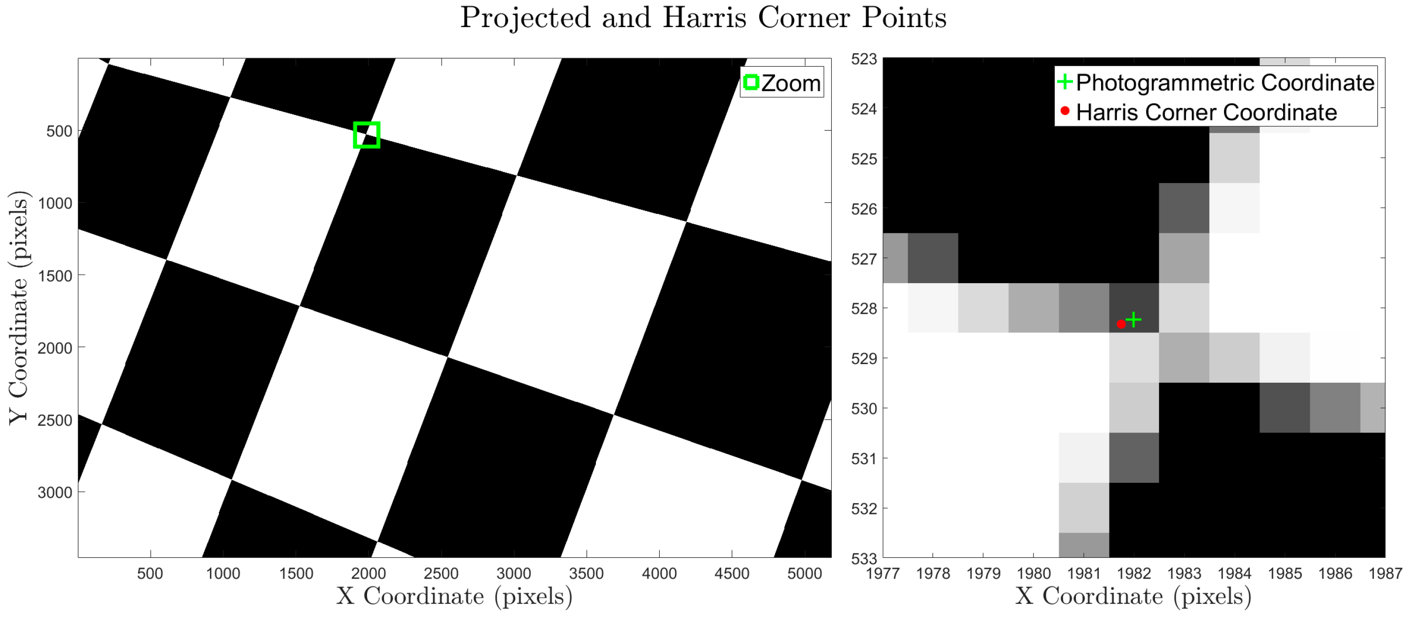
The first validation experiment was designed to ensure that the camera interior and exterior orientation were set accurately using a pinhole camera model. The pinhole camera model represents an ideal test case and is commonly the output from render engines. While Vertex Shaders algorithms can be programmed and implemented into a Computer Graphics workflow to accurately simulate lens distortion, the programming and implementation of this method is time consuming and can be confusing for someone not familiar with computer graphics. A pinhole camera model was used for this experiment to validate the photogrammetric accuracy of the Blender Render Engine. This initial experiment was performed by creating a simple scene consisting of a 1000 m3 cube with a 10 × 10 black-and-white checkerboard pattern on each wall, as depicted in Figure 1. The corner of each checkerboard was defined to have known 3D world coordinates. A series of images was rendered using various camera rotations, translations, focal lengths, sensor sizes, and principal point coordinates. To ensure that the images were rendered correctly, the coordinates of the checkerboard corners were calculated from the rendered imagery using a corner feature detector and compared to the expected coordinates of the targets using photogrammetric equations. The differences between the image-derived coordinates and the photogrammetric equation derived coordinates should have a mean of 0 in both dimensions, and a subpixel variance on the order of the accuracy of the image corner feature detector.
To validate the photogrammetric projection accuracy of the Blender Internal Render Engine using this experiment, a 1000 m3 cube was placed with the centroid at the coordinate system origin. Five hundred images were rendered using five different interior orientations and random exterior orientations throughout the inside of the cube. These parameters were input using the Blender Python API, with the ranges of each input parameter shown in Table 1. The accuracy of the imagery was first assessed qualitatively by plotting the photogrammetrically-calculated points on the imagery in MATLAB (e.g., green plus symbol in Figure 1, right). Once the rough accuracy was confirmed, a nearest neighbor was used to develop correspondences between the Harris corner coordinates and the photogrammetric equation derived coordinates. The mean and variance of the differences between the correspondences in each experiment are shown in Table 2.
Although the bias and standard deviation were quite small, it was of interest to go a step further and determine the extent to which the small errors were attributable to the Harris corner detector, rather than the render engine. To this end, an additional test was performed using 1000 simulated checkerboard patterns, generated with random rotations, translations, and skew to create a synthetic image dataset. The known coordinates of the corners were compared to the coordinates calculated with the Harris Corner feature detector, producing the results shown in Table 3. The variance from synthetic imagery dataset was found to account for approximately 75% of the variance in the Blender simulations. The remaining ~0.07-pixel variance could be attributed to mixed pixels in the Blender simulation, antialiasing effects in the Blender simulation, or simply an amount of variability that was not fully encompassed with the various affine transformations that were applied to the synthetic imagery. For this experimentation, this level of accuracy was deemed acceptable, as errors being investigated are likely to be at least an order of magnitude larger.
2.3. Point Spread Function
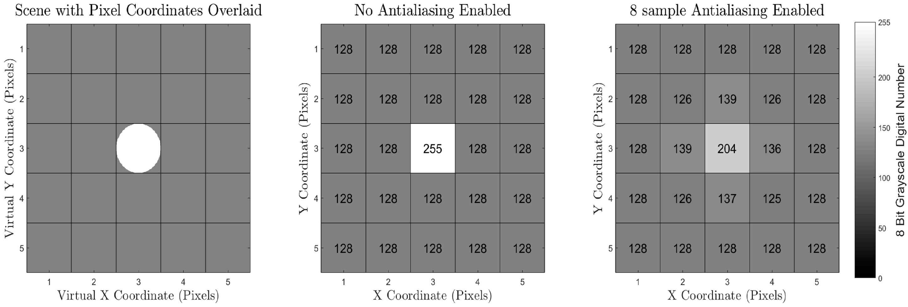
The second validation experiment was designed to ensure that no unintended blurring was applied to the rendered image. (Later, purposefully-introduced motion and lens blur will be discussed.) Ideally, the point spread function (PSF) of the renderer would be a unit impulse, indicating no unintended blurring. The test for this condition was performed by simulating a white circular plane placed at a distance and size such that it existed in only one pixel. The rendered image of this object should not be blurred into surrounding, background pixels. This test is of particular importance when antialiasing is performed, as the super-sampling pattern and filter used to combine the samples can sometimes create a blurring effect. For example, the default antialiasing in Blender uses a “distributed jitter” pattern and the Mitchel–Netravali filter [28], which uses super-sampled values from neighboring pixels to calculate a pixel value. This effect can be seen in Figure 2, where the intensity of the white plane has influenced all eight of the neighboring pixels, even though the plane should only be visible in one pixel. While the photographic inaccuracy for this example is minimal, larger errors resulting from different filters could propagate into the resultant SfM derived point cloud, especially when fine-scale textures with high gradients are used.
To perform this test using the Blender Internal Render Engine, a sensor and scene were set up such that the geometry of the circular plane was only captured with one pixel in the render of a 5 × 5 pixel image. The logic of this experiment was that any other pixels containing values different than the background digital number of 128 indicated a potential blurring artifact of the rendering. Rendered imagery is shown with and without antialiasing in Figure 2. The antialiasing used the default settings for the Blender Internal Render Engine (8 Samples, Mitchell–Netravali filter). The rendered image with no antialiasing was found to contain no blurring of the image, while the antialiased image contained a slight amount of blurring. Note that the theoretical pixel value should be ~227 (based on the proportion of the grey center pixel filled by the white circle in the leftmost subfigure), and neither sampling methodology perfectly represents the scene. The antialiased imagery super-samples the scene and renders a smoother, more photorealistic imagery, and was deemed to be suitable for purposes of this work.
2.4. Texture Resolution
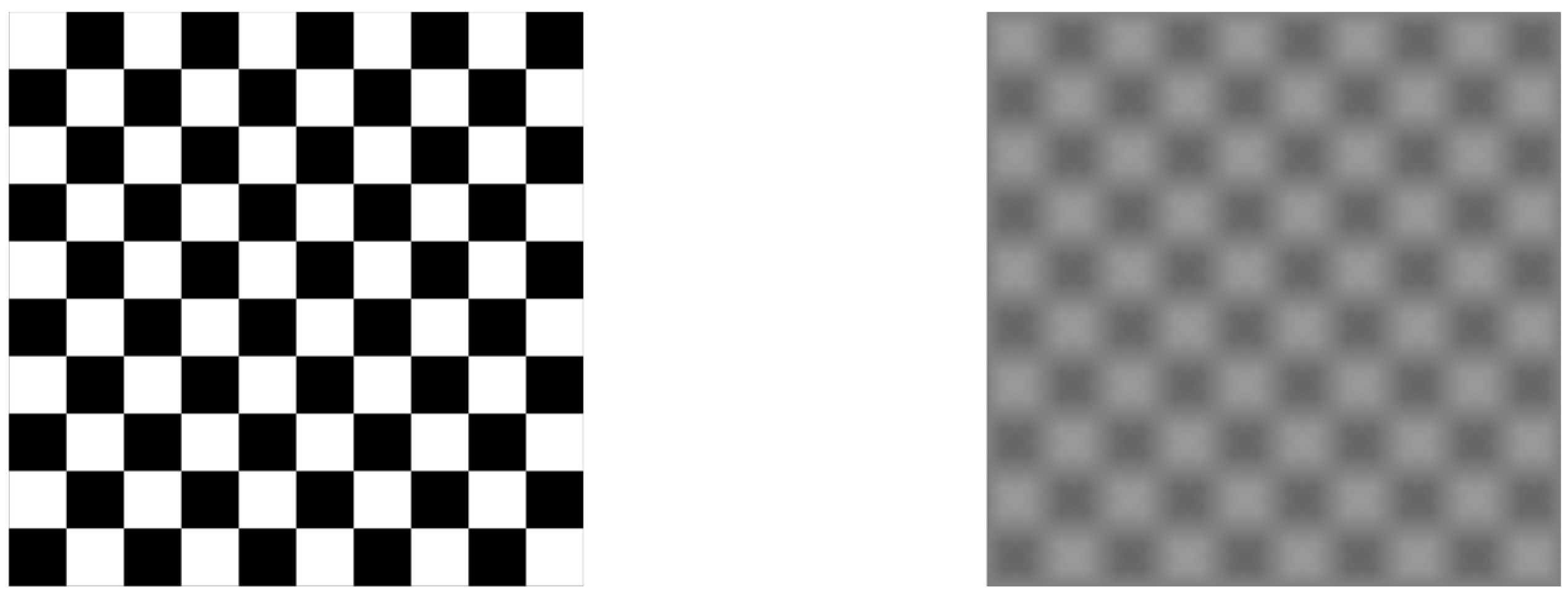
The final validation experiment ensured that any textures applied to the objects in the scene were applied in a manner which maintained the resolution of the imagery without compression or subsampling. This validation experiment was performed by applying a texture on a flat plane and rendering an image containing a small number of the texture pixels. The image was then visually assessed to verify that the desired number of pixels were in the frame and that no smoothing was applied. When rendering textures in computer graphics, there is an option to perform interpolation, yielding a smoother texture. This is sometimes desired to create more realistic scenes. An example of a texture with and without interpolation is shown in Figure 3.
To validate the texture resolution of the Blender Internal Render Engine, a black-and-white checkerboard pattern in which each checkerboard square was 1 × 1 texel was applied to a flat plane, such that each texel represented a 10 cm × 10 cm square. An image was rendered using a focal length and sensor size such that each texel was captured by 100 × 100 pixels, as shown in Figure 3 with and without interpolation. The rendered images were qualitatively observed, and it was determined that the rendering had not subsampled or compressed the texture image.
2.5. Use Case Demonstration
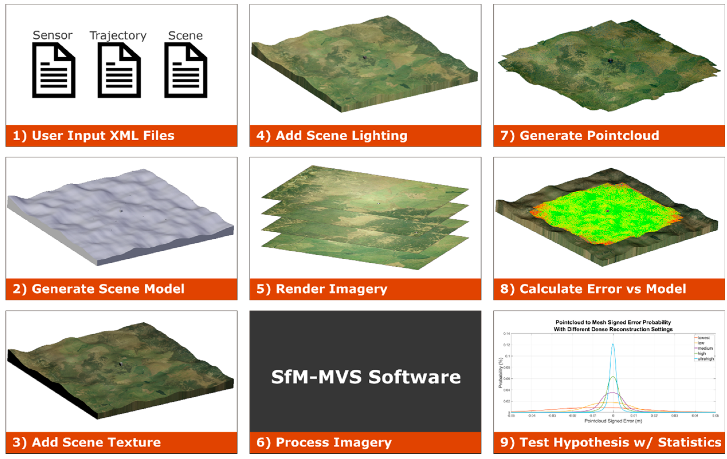
An example experiment was designed as a proof-of-concept to demonstrate the usefulness of the simUAS simulated imagery rendering workflow for testing the effect of various independent variables on SfM accuracy. This experiment was specifically designed to observe how the dense reconstruction quality setting in Agisoft Photoscan Pro [29] affects the dense point cloud accuracy and to test the statement made in the user manual that a higher dense accuracy setting produces more accurate results [30]. The scene, texture, lighting, camera, and camera positions were selected with the intention of simulating a common UAS flight scenario. These parameters were input using a custom XML schema and the Blender Python API. The simUAS processing and analysis workflow is shown in Figure 4. The computer used to render and process the data for this experiment was a Windows 7 Desktop PC with an Intel Xeon CPU (E5-1603 @ 2.80 GHz), GeForce GTX 980 graphics card (4 Gb), and 32 Gb of RAM.
2.6. Use Case Experiment Design
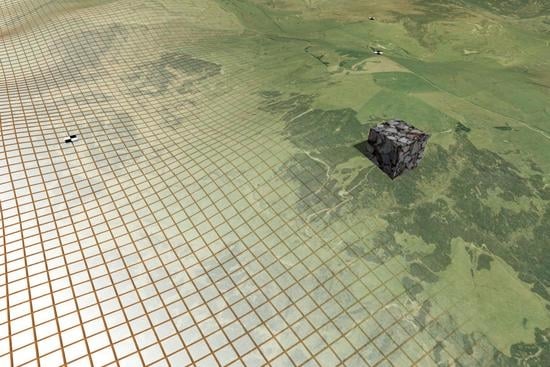
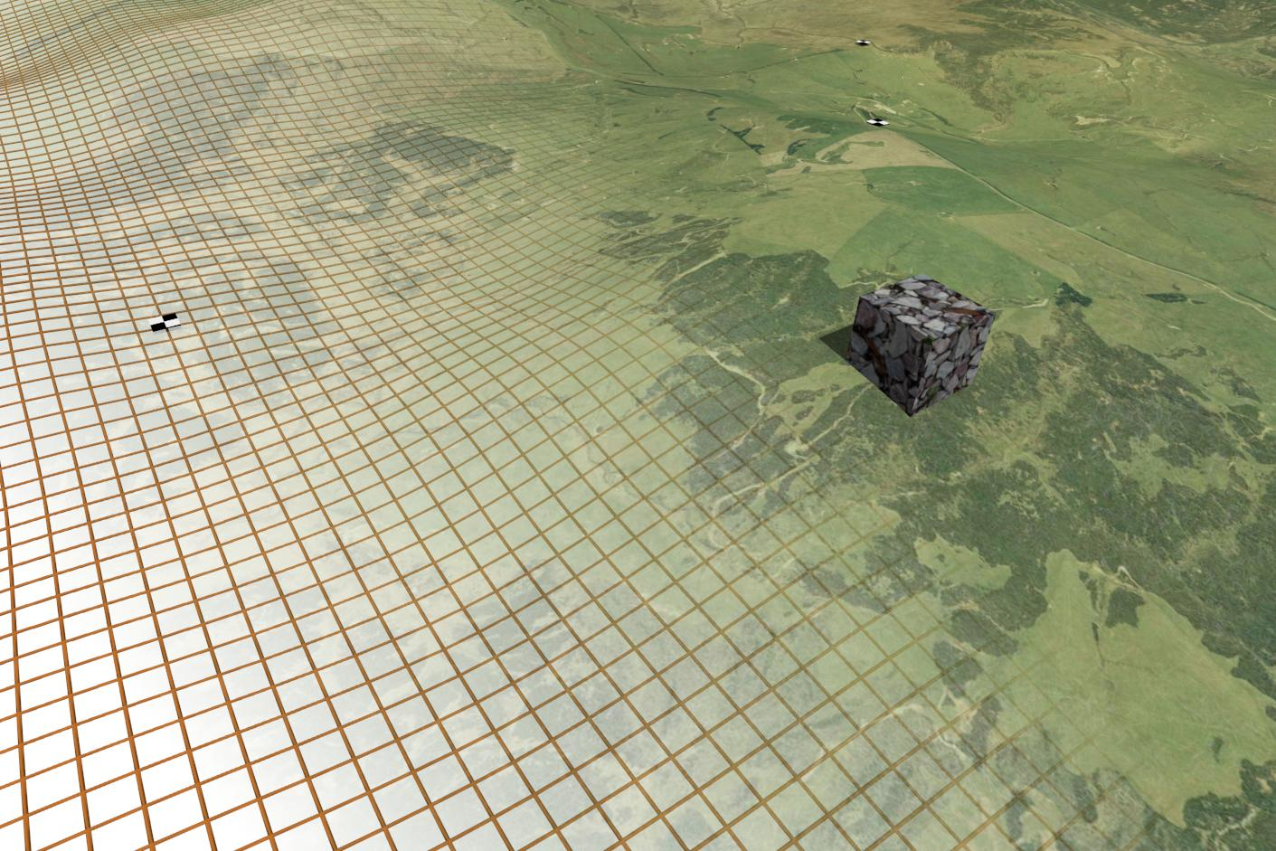
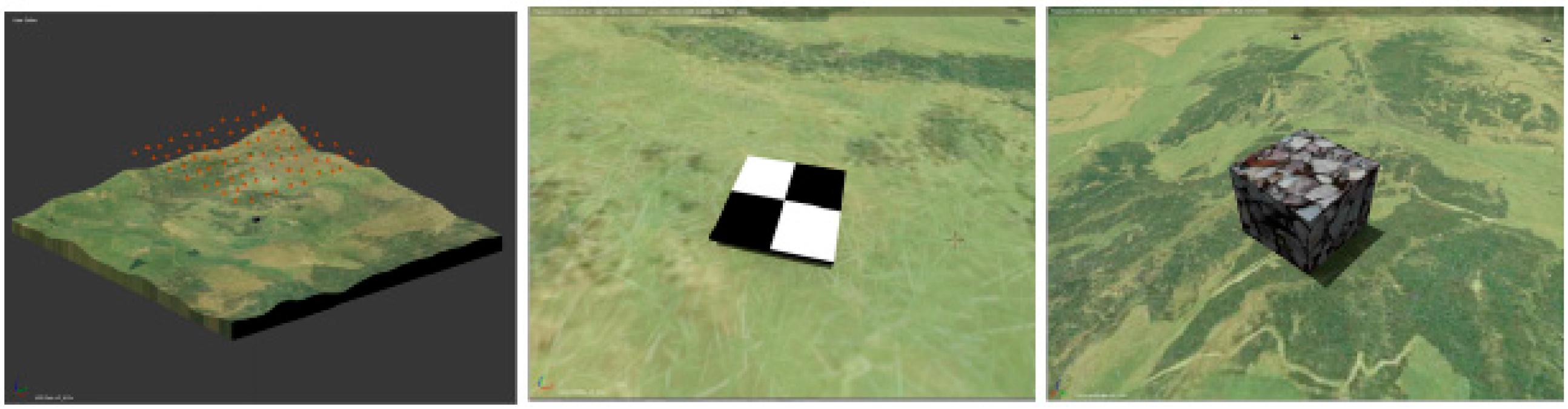
A 200 m × 200 m square mesh was generated to simulate a topography with rolling hills using a 1 m grid. A large (27 m3) cube was placed in the center of the scene to test surface reconstruction accuracy on regions with sharp corners and edges. Ten 1 m × 1 m × 0.05 m square, checkerboard pattern GCPs were distributed evenly throughout the scene 0.25 m above the ground surface. The materials of all objects in the scene were modeled as perfect Lambertian surfaces. The topographic surface was textured using a combination of two textures. The first texture was a 7200 × 7200 pixel aerial image [31] for an effective texel footprint with a linear dimension of 2.78 cm. The second texture was a 3456 × 3456 pixel image of grass was tiled ten times in both the x and the y dimensions for an effective repeating image pattern 34,560 × 34,560 pixels, and a texel footprint with a linear dimension of 0.58 cm on the topography. The image of grass was taken with a DSLR camera (Canon T5i) and manually edited to create a seamless texture for tiling with no edge effects between tiles. The aerial image and grass texture were merged together by setting the grass texture with an alpha of 0.15 and the aerial image layered beneath it with an alpha value of 1. The cube was textured using a 3456 × 3456 pixel seamless image of rocks that was derived from a DSLR (Canon T5i) image taken by the authors. This resulted in an effective texel footprint with a linear dimension of 0.35 cm on the cube. Each of the textures was set so that the coloring on the scene was interpolated between texels and there were no unrealistic edge effects. The texel footprint of each of the materials is set to a value less than the GSD, which, as described below, is 1.00 cm. Oblique images of each object in the scene are shown in Figure 5.
The scene was illuminated using a “Sun” style of lamp in Blender, where all the light rays are parallel to one another. The light was initially directed at nadir, and the angle was linearly interpolated to a 30-degree rotation about the x-axis for the final image. This varying sun angle simulates the slight movement of shadows, as is experienced in a real world data acquisition. If desired, further control over the illumination settings within the render engine could be achieved using the “color management” settings. Regions that are shadowed from the sun in the Blender Internal Render Engine receive no light; hence to more realistically model ambient light within the scene and improve texture in shadowed regions, an ambient light source was added. These settings generated a scene with adequate lighting on all objects in the scene. (For a test in which illumination is one of the primary variables investigated, additional refinement of the illumination parameters in this step is recommended.)
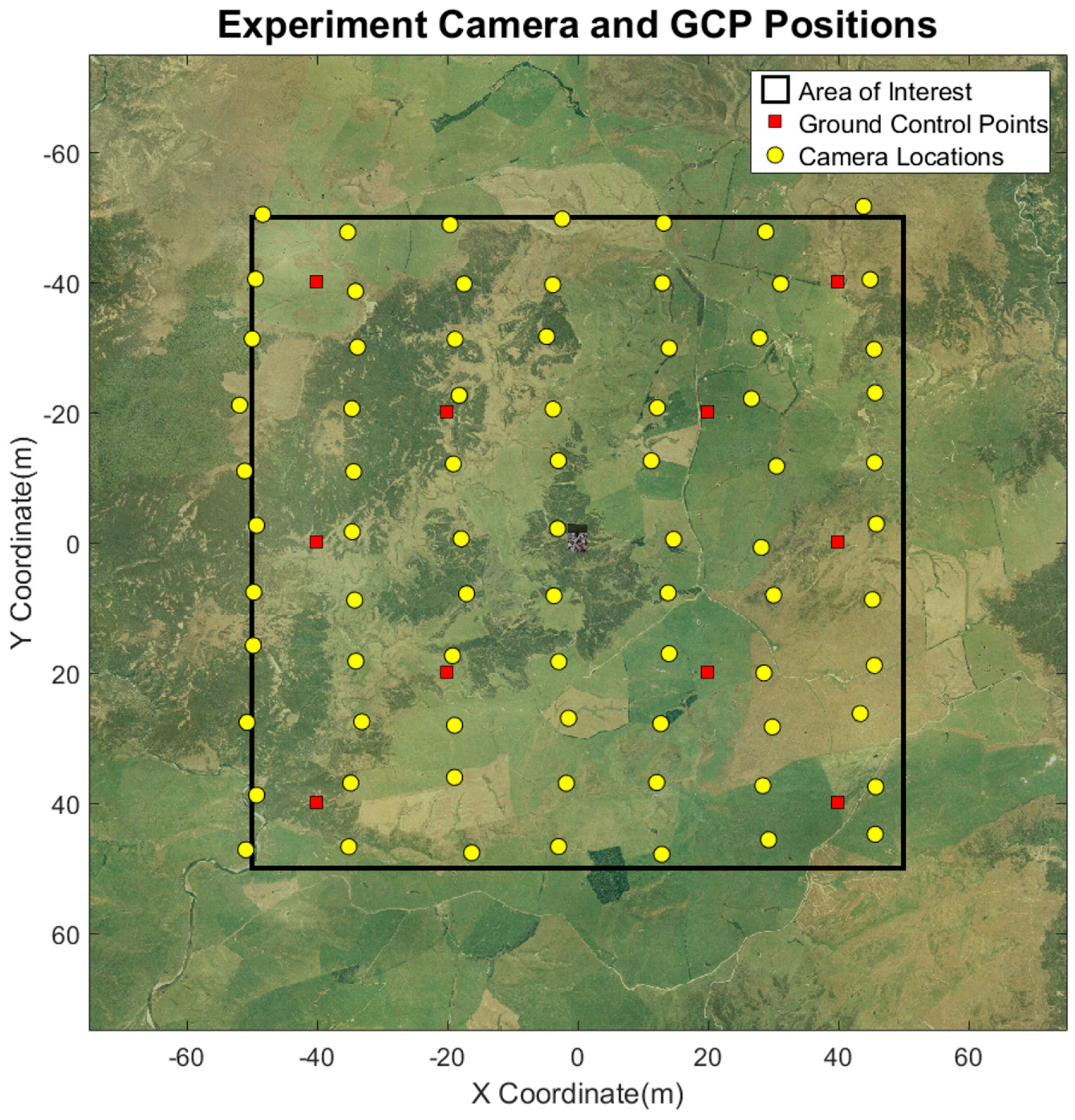
A camera was created in Blender with parameters meant to emulate a Sony A5000 camera with a 16-mm lens and 5456 × 3632 (20 Mp) pixel sensor. This particular camera was chosen, as it is a popular choice for UAS imagery acquisition. An array of simulated camera stations was placed on a flight path to create a ground sampling distance (GSD) of 1.00 cm and an overlap and sidelap of 75% each. To remove imaging on the edge of the simulated topographic surface, the inner 100 m × 100 m of the topography was selected as the area of interest (AOI). The trajectory consisted of 77 simulated camera stations distributed across 7 flight lines with nadir looking imagery, as shown in Figure 6. To generate imagery that was more representative of a real-world scenario with a UAS, white Gaussian noise (σ = 1 m) was added to the camera translation in each of the three dimensions to simulate uncertainty in the true UAS trajectory due to UAS navigation GPS uncertainty. This uncertainty was added to the actual position of the simulated camera when the image was rendered, and was accounted for in the reported trajectory used in SfM processing. White Gaussian noise (σ = 2°) was also added to the camera rotation about each of the three axes to simulate a UAS which does not always take perfectly nadir imagery. Imagery was then rendered using Blender Internal Render Engine with the default eight-sample antialiasing enabled. The processing to render the imagery took 2 h and 50 min on the workstation described earlier.
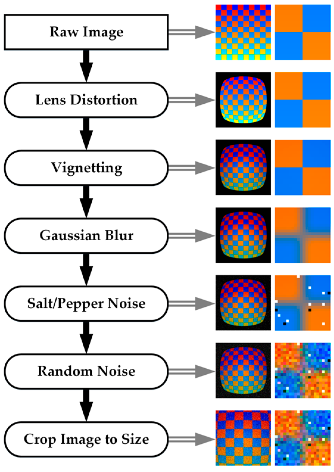
The imagery output from Blender, rendered using a pinhole camera model, was post-processed in MATLAB to simulate various camera and lens effects. These effects generate imagery that is more representative real world imagery, and can have a significant effect on the quality of the SfM and MVS pointcloud accuracy. Nonlinear brown distortion was first applied by shifting the original pixel coordinates using Equations (1)–(3) [32], and reinterpolating the image intensity values onto a rectilinear grid. Vignetting (Equation (4)), Gaussian blur, salt-and-pepper noise, and Gaussian noise, were then applied to the imagery. To accurately apply fisheye distortion and Gaussian blur, the imagery was rendered at a larger sensor size than the desired output sensor size, and then cropped after the filtering was applied. A flowchart depicting the postprocessing steps is shown in Figure 7. The constants used in this post-processing are shown in Table 4. The post-processing of imagery in MATLAB took 50 min.
2.7. Use Case Processing Methodology
The resultant imagery was processed using the commercial software Agisoft Photoscan Pro using the settings shown in Table 5. The dataset was processed by inputting the position of the cameras, the position of the GCPs, and the camera calibration file. Additionally, the pixel coordinates of the GCPs, which are traditionally clicked by the user with varying degrees of accuracy, were calculated using photogrammetric equations and input into the program. A nonlinear adjustment was performed using the “optimize” button, and the reported total RMSE for the GCPs was 0.38 mm. It is important to note that we purposefully eliminated additional sources of uncertainty that exist in field-based studies, such as uncertainties in the surveyed points, the GPS reported UAS position, the manual digitization of pixel coordinates for GCPs, and in the calculation of the camera calibration, in order to isolate the specific variable being investigated.
A dense reconstruction was performed using the “aggressive” filtering and each of the quality settings available in Photoscan (lowest, low, medium, high, and highest) to generate five different point clouds. According to the Photoscan documentation, the higher is the quality setting, the more “detailed and accurate” is the generated geometry. The limiting factor is the time and CPU processing power required to process large datasets. Ultrahigh becomes quickly unattainable to users without purpose-built CPUs and GPUs with a large amount of RAM. The processing time and number of points for each point cloud are shown in Table 6. A more detailed discussion of the accuracy of each pointcloud is included in Section 3.
Each of the dense point clouds was processed using CloudCompare [33] and compared to the ground truth blender mesh using the CloudCompare “point to plane” tool. This tool calculates the signed distance of every point in the point cloud to the nearest surface on the mesh, using the surface normal to determine the sign of the error. Each point cloud was then exported and analyzed in MATLAB to determine how the dense reconstruction quality setting affects the point cloud error.
3. Use Case Results
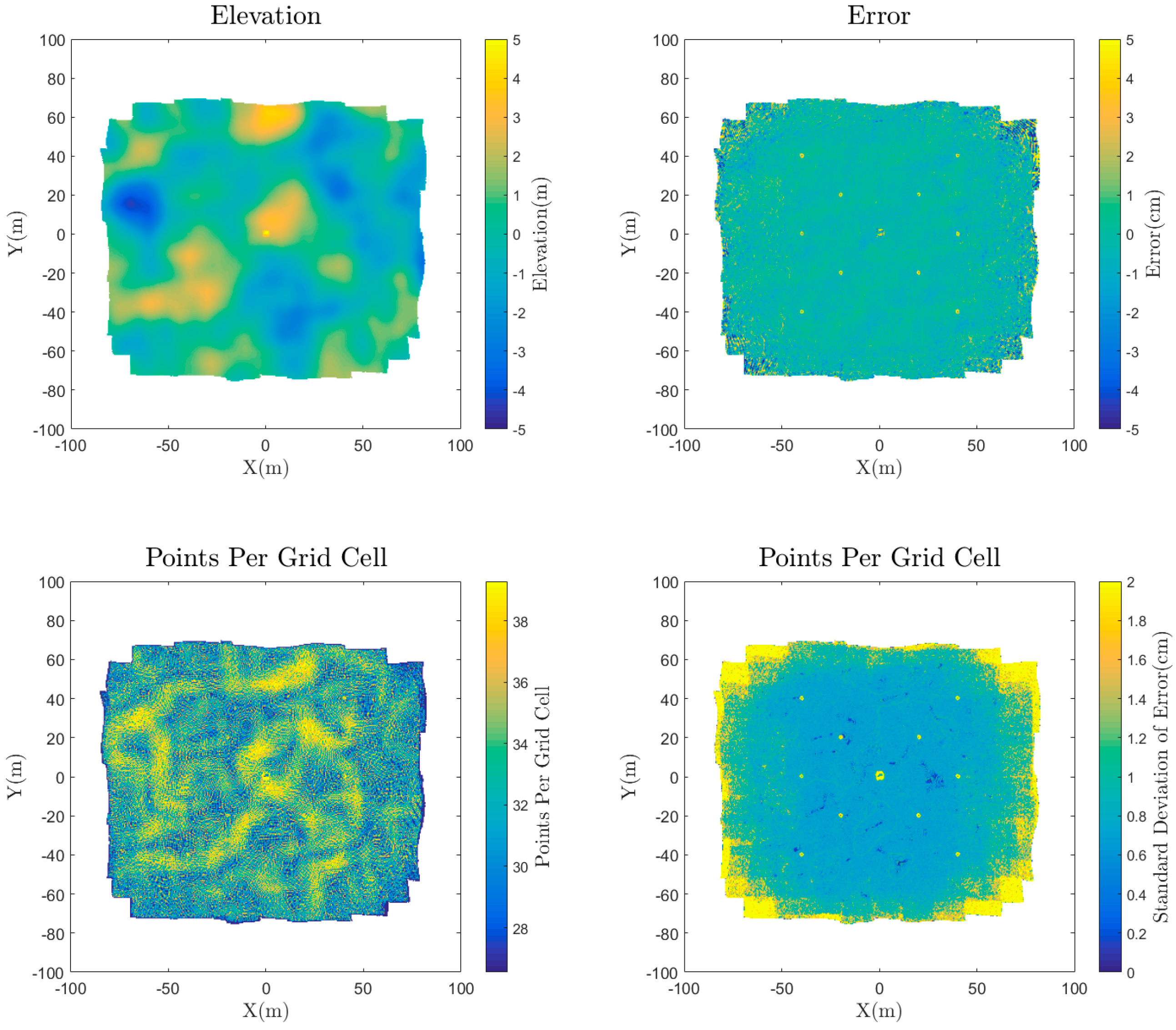
The error was first visualized spatially for each reconstruction by gridding the point cloud elevation and error using a binning gridding algorithm, where the value of each grid cell is calculated as a mean of all the points located horizontally within that grid cell. The number of points and standard deviation of points in each grid cell were also visualized. The results for the medium quality dense reconstruction are shown in Figure 8. These plots are useful to begin to explore the spatial variability in both the density and the errors in the data. One initial observation for this dataset is that there is a larger standard deviation of error at the edges of the point cloud outside the extents of the AOI. This is due to the poor viewing geometry at the edges of the scene, and suggests that in practice these data points outside of the AOI should be either discarded or used cautiously.
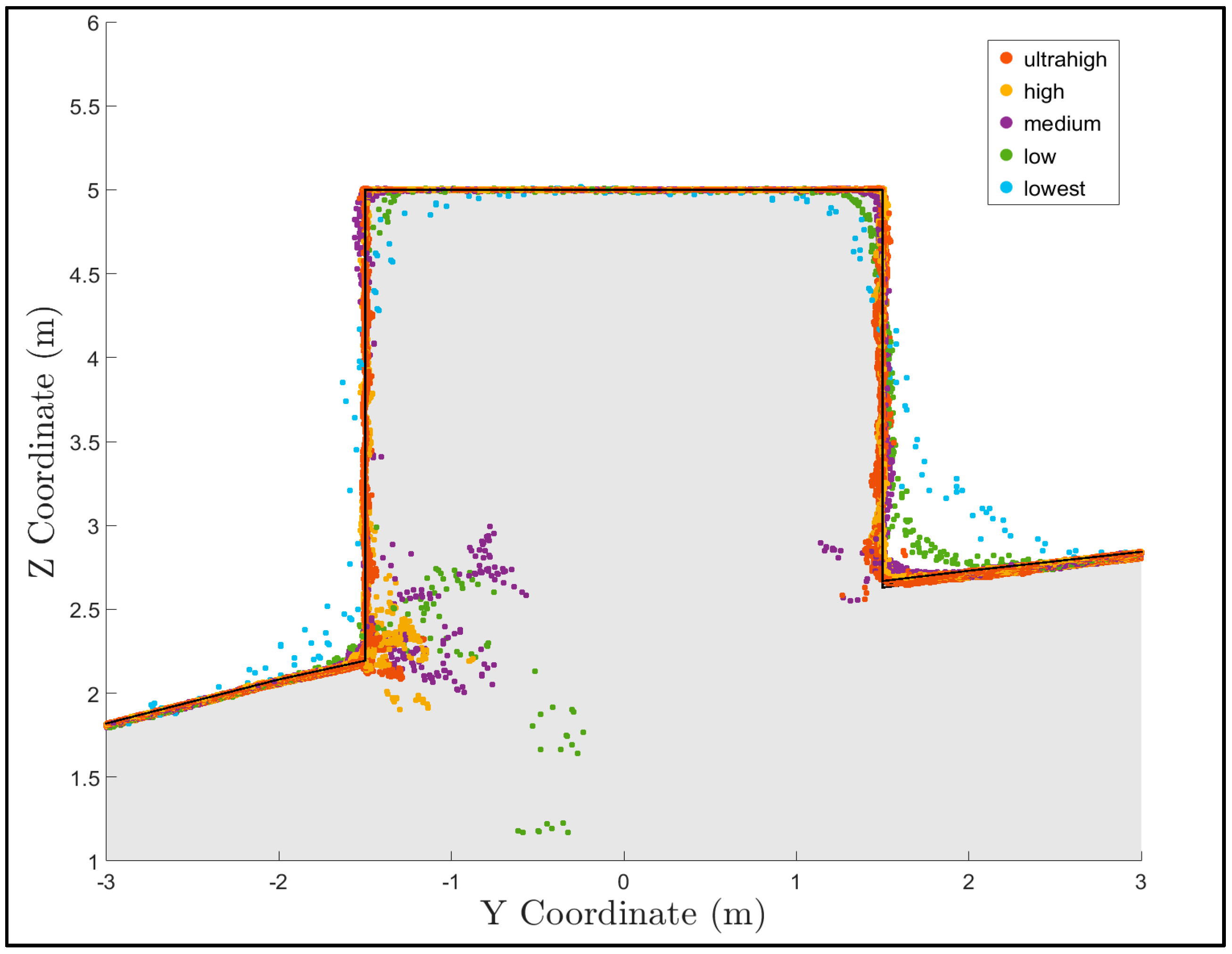
To qualitatively observe the effect of different quality dense reconstructions, a plot showing the true surface and the points from each construction in a 0.5-meter-wide section of the 27 m3 box is shown in Figure 9. Notice that the accuracy of each point cloud at the sharp corners of the box improves as the quality of the reconstruction increases, which is consistent with the Agisoft Photoscan Pro manual [30]. This observation suggests that higher quality dense reconstruction settings will increase accuracy in regions with sharp corners.
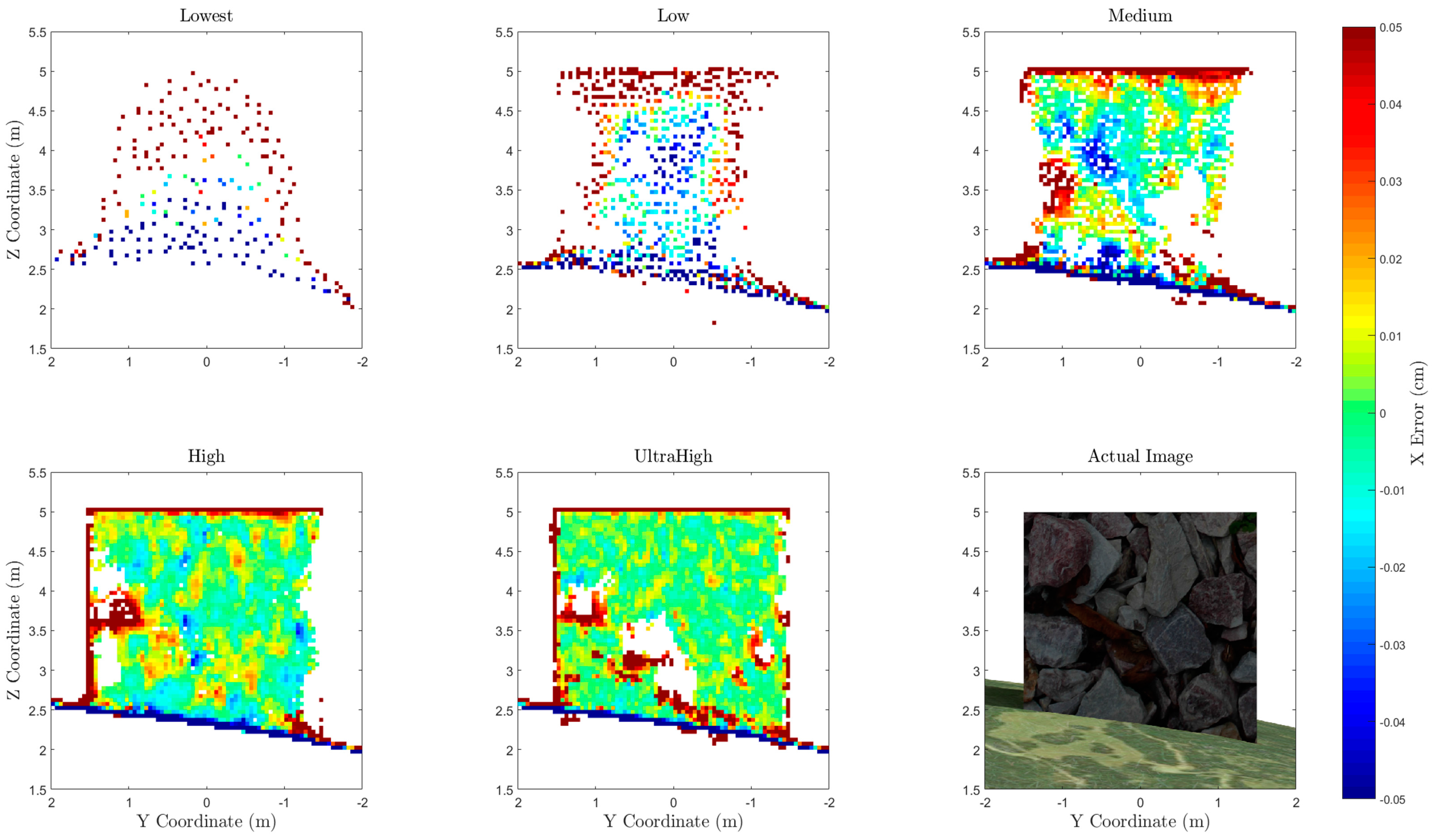
A visualization of the horizontal error of points along one side of the box is shown in Figure 10. All points within 0.25 m horizontally of the face of the box were compared to the true x coordinate of the box face and gridded at 0.05-m resolution. This 1D error calculation along the x dimension shows how well the face of the box is captured in the point cloud. Note that errors along the edge of the box and along the ground surface should be ignored, as these grid bins on the edge represent areas where the average coordinate will not be equal to the coordinate of the side of the box, even in an ideal case. The regions that are white indicate an absence of data points. The size and location of these data gaps varies between each point cloud. For example, the high-quality setting point cloud contains points in the lower center of the cube, while the ultra-high does not. While the data gap in the ultra-high appears to be correlated to a region of low texture on the actual image, further research is required to definitively determine the cause.
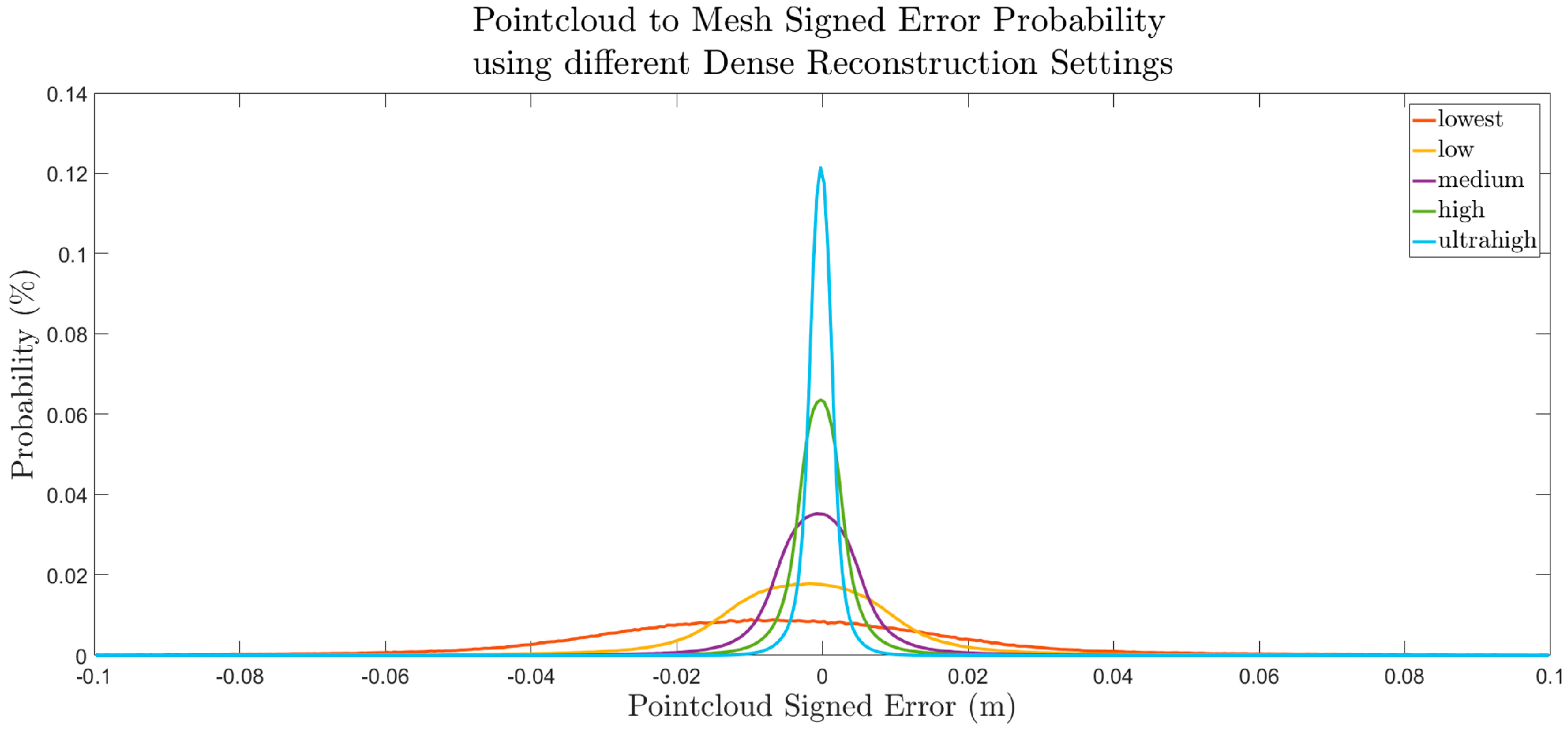
A more quantitative, statistical assessment was performed to assess the error throughout the entire scene by calculating a histogram for the distribution of error in each point cloud, as shown in Figure 11. These distributions bolster the conclusion derived from the box profile plot, which is that higher quality dense reconstruction settings yield more accurate results than a lower quality reconstruction. While the accuracy of the GCPs, as provided in Agisoft Photoscan, averaged 0.38 mm (RMSE), the standard deviations of the points from the dense reconstruction ranged from 2.6 mm to 32.3 mm, as shown in Table 6. This observation indicates that the GCP accuracy table is insufficient as a metric to depict the accuracy of the resultant dense point cloud. While these conclusions suggest general trends, further experimentation is required for error distributions to be generalized. The magnitude of the error was likely influenced by the varying sun angle, image noise, image blur, and image vignetting, which were introduced to model the simulated camera more realistically. These variables could be isolated individually in future experimentation.
4. Discussion
The use case demonstration provides just one example of the type of rigorous analysis that can be obtained by utilizing the simUAS image rendering workflow. It is important to note that the results of this experiment are closely coupled to the texture and topography of the scene. Future work will vary these independent variables to assess their effect on point cloud accuracy.
The first conclusion from this example experiment is that the error and standard deviation of error are larger for points outside of the area of interest, which in this experiment was −50 m to 50 m in both the x and y directions. This is shown in the spatial error plot in Figure 8. The cause of this error is the poor viewing geometry for imaging these points, where they are only seen at a few camera stations and, even then, only at oblique angles. In practice, these points should be included in the final data product with caution, as it is shown here that the errors can be significantly greater than those within the AOI.
The second conclusion from this example experiment is that a “higher” quality dense point cloud reconstruction setting results in a more accurate point cloud, as shown qualitatively in Figure 9 and Figure 10, and quantitatively in Figure 11. The quality settings in Photoscan determine the amount of downsampling of the imagery that should occur before performing the reconstruction algorithm. The downsampling of the imagery removes some of the finer texture details in the imagery, and therefore reduces the quality of the keypoint matching. The authors recommend using the “highest” quality dense reconstruction setting that the computer processing the dataset can handle. However, if there are noticeable data gaps in the point cloud, one should consider processing the point cloud on a lower dense reconstruction setting and merging the point clouds. For this experiment, a relatively small number of 20 Mp images (77) were used to create the dense point cloud, which took almost 12 hours for the highest point cloud setting. The resultant point cloud for this setting also contained 186 million points, which caused some point cloud data viewers and processing to fail, due to memory issues. For this reason, ultra-high may not be a viable solution for all experiments.
The third conclusion is that the RMSE of the GCP control network as shown in Agisoft Photoscan Pro is insufficient to characterize the accuracy of the resultant dense point cloud. In this extremely idealized experiment, where the GCP positions, pixel coordinates of GCPs, camera positions, and camera calibration were all input precisely, the GCP control network 3D RMSE reported by Agisoft Photoscan was 0.38 mm. The smallest standard deviation, which occurred using the “ultra-high” quality setting, was 2.6 mm and the largest standard deviation, using the “lowest” setting, was 32.3 mm, as shown in Table 6. Further experimentation is needed to determine the relationship between the Photoscan reported GCP total RMSE and the computed RMSE of the dense point cloud. The image rendering workflow developed in this research is well suited to perform this experimentation, which is currently being considered as one of a number of planned follow-on studies.
Methodology Implications
This methodology generates photogrammetrically-accurate imagery rendered using a pinhole camera model of a scene with various textures and lighting, which is then processed to assess SfM point cloud accuracy. The rendered imagery can be processed to add noise, blur, nonlinear distortion, and other effects to generate imagery more representative of that from a real-world scenario prior to SfM processing. The accuracy of the camera trajectory, GCP position, camera calibration, and GCP pixel coordinates in each image can also be systematically adjusted to simulate uncertainty in a real-world scenario. The ability to adjust these parameters enables a user to perform a sensitivity analysis with numerous independent variables.
While this methodology enables the user to perform repeatable, accurate experiments without the need for time-consuming fieldwork, there are currently some limitations in the experiment methodology when utilizing the Blender Internal Render Engine. First, the internal render engine does not handle global illumination, and therefore light interactions between objects are not modeled. A second limitation of the lighting schema is that the radiometric accuracy has not been independently validated. There are a few methods within the render engine which effect the “color management” of the resultant imagery. For this experiment, these settings were left at the default settings, providing imagery that was not over- or underexposed. While the lighting in the scene using the Blender Internal Render Engine does not perfectly replicate physics-based lighting, the absolute color of each surface of an object is constant and perfectly Lambertian. The keypoint detection and SfM algorithms utilize gradients in colors and the absolute colors of the scene, and the accuracy of the methodology should not be effected by the imperfect lighting; however, it is recommended that this be rigorously investigated in future research.
Another source of inaccuracy in the Blender Internal Render Engine methodology is that the methodology to convert the scene to pixel values relies on an integration over a finite number of subpixel super-sampling ray calculations. This deviates from a real-world camera where the pixel value is a result of an integration over all available light. The Blender Internal Render Engine uses the term “antialiasing” to describe a super-sampling methodology for each pixel, which can super-sample up to 16 samples per pixel. This small, finite number of samples per pixel can induce a small amount of inaccuracy when mixed pixels are present. These inaccuracies, though, are small enough to be deemed negligible for most experiments which are expected to be undertaken using the workflow presented here.
However, another potential source of uncertainty induced into the system is the use of repeating textures to generate a scene. In the use case provided earlier, the grass texture was repeated 10 times in both the x and y directions. This repeating pattern was overlaid onto another image, to create different image color gradients in an attempt to generate unique texture features without requiring an extremely large image as the texture. Despite this effort, it is possible that keypoint detection and matching algorithms could generate false positives which may bias the result if not removed or detected as outliers. This phenomenon could also occur in a real-world scenario, where manmade structures often exhibit a repeating pattern of similar shapes and colors. In this experiment, this effect was not observed, but if the scene is not generated carefully, these repeating textures could induce a significant amount of inaccuracy in the SfM processing step.
5. Conclusions
This study has demonstrated a new workflow leveraging the Blender Internal Render Engine, an open-source computer graphics render engine, to generate simulated UAS imagery data sets for rendered scenes, suitable for input into SfM-MVS software. The output point clouds can be compared against ground truth (which is truly the “truth,” in this case, as GCPs, check points and other features have been synthetically placed in the scene with exact coordinates) to perform accuracy assessments. By purposefully and systematically varying different input parameters, including modeled camera parameters (e.g., focal length and resolution), modeled acquisition parameters (e.g., flying height and exposure rate), environmental parameters (e.g., solar illumination angle), and processing parameters (e.g., reconstruction settings), sensitivity analyses can be performed by assessing the change in accuracy as a function of change in each of these parameters. In this way, hundreds of experiments on UAS imagery processed in SfM-MVS software can be performed in the office, without the need for extensive, costly field surveys. An additional advantage of the simUAS image rendering approach is that it avoids confounding variables (e.g., variable wind and solar illumination, as well as moving objects in the scene), which can complicate accuracy assessments performed with real-world imagery.
In this paper, one example of a use case was presented, in which we examined the effects of the Agisoft Photoscan reconstruction quality setting (lowest, low, medium, high, and highest) on resultant point cloud accuracy using a simulated UAS imagery data set with a camera model emulating a Sony A5000. It was shown that the RMSE of the resultant point clouds does, in fact, depend strongly on the reconstruction quality setting. An additional finding was that the data points outside of the AOI should be either discarded or used with caution, as the accuracy of those points is higher than that of the point cloud within the AOI. While these results are informative (if, perhaps, not entirely unexpected), it is important to note that this is just one of a virtually limitless number of experiments that can be run using the workflow presented here. The project team is currently planning to use the simUAS workflow to examine point cloud accuracy achievable with new sensor types, and also to conduct accuracy assessments of shallow bathymetric points in SfM-MVS point clouds generated from UAS imagery.
Additional topics for future work include investigating the radiometric fidelity of the simulated imagery, and further assessing the impacts of texture and topography in the simulated scenes. More advanced post-processing effects will be explored, including local random variability from the Brown distortion model and lens aberration (spherical and chromatic). Alternative render engines will also be investigated for feasibility, using the validation methodology described here. As SfM-MVS algorithms are continually being improved, it is also of interest to use this methodology to test new SfM-MVS software packages, both commercial and open source. Another extension of the current work would include using the procedure presented here to simulate imagery acquired not only from UAS, but also vehicles, boats, or handheld cameras. It is anticipated that these procedures will prove increasingly beneficial with the continued expansion of SfM-MVS algorithms into new fields.
Acknowledgments
Funding for this project (including open access publication) was provided internally by the School of Civil and Construction Engineering at Oregon State University. A portion of the first author’s time was supported by Grant Number G14AP00002 from the Department of the Interior, United States Geological Survey to AmericaView. The contents of this publication are solely the responsibility of the authors; the views and conclusions contained in this document are those of the authors and should not be interpreted as representing the opinions or policies of the U.S. Government. Mention of trade names or commercial products does not constitute their endorsement by the U.S. Government.
Author Contributions
R.K.S. conceived of and coded the simUAS workflow. C.E.P. supervised the research and participated in experiment design and analysis of results. Both authors contributed to writing the paper.
Conflicts of Interest
The authors declare no conflict of interest.
References
- Westoby, M.J.; Brasington, J.; Glasser, N.F.; Hambrey, M.J.; Reynolds, J.M. “Structure-from-Motion” photogrammetry: A low-cost, effective tool for geoscience applications. Geomorphology 2012, 179, 300–314. [Google Scholar] [CrossRef]
- Fonstad, M.A.; Dietrich, J.T.; Courville, B.C.; Jensen, J.L.; Carbonneau, P.E. Topographic structure from motion: A new development in photogrammetric measurement. Earth Surf. Process. Landforms 2013, 38, 421–430. [Google Scholar] [CrossRef]
- Ullman, S. The Interpretation of Visual Motion; MIT Press: Cambridge, MA, USA, 1979. [Google Scholar]
- Ullman, S. The Interpretation of Structure from Motion. Proc. R. Soc. B Biol. Sci. 1979, 203, 405–426. [Google Scholar] [CrossRef]
- Wolf, P.R.; Dewitt, B.A. Elements of Photogrammetry: With Applications in GIS; McGraw-Hill: New York, NY, USA, 2000. [Google Scholar]
- Lowe, D.G. Distinctive image features from scale invariant keypoints. Int. J. Comput. Vis. 2004, 60, 91–110. [Google Scholar] [CrossRef]
- Clapuyt, F.; Vanacker, V.; Van Oost, K. Reproducibility of UAV-based earth topography reconstructions based on Structure-from-Motion algorithms. Geomorphology 2015, 260, 4–15. [Google Scholar] [CrossRef]
- Furukawa, Y.; Hernández, C. Multi-View Stereo: A Tutorial. Available online: http://0-dx-doi-org.brum.beds.ac.uk/10.1561/0600000052 (accessed on 20 April 2017).
- Eltner, A.; Kaiser, A.; Castillo, C.; Rock, G.; Neugirg, F.; Abellán, A. Image-based surface reconstruction in geomorphometry-merits, limits and developments. Earth Surf. Dyn. 2016, 4, 359–389. [Google Scholar] [CrossRef]
- Smith, M.W.; Vericat, D. From experimental plots to experimental landscapes: Topography, erosion and deposition in sub-humid badlands from Structure-from-Motion photogrammetry. Earth Surf. Process. Landforms 2015, 40, 1656–1671. [Google Scholar] [CrossRef]
- Dandois, J.P.; Olano, M.; Ellis, E.C. Optimal altitude, overlap, and weather conditions for computer vision uav estimates of forest structure. Remote Sens. 2015, 7, 13895–13920. [Google Scholar] [CrossRef]
- Colomina, I.; Molina, P. Unmanned aerial systems for photogrammetry and remote sensing: A review. ISPRS J. Photogramm. Remote Sens. 2014, 92, 79–97. [Google Scholar] [CrossRef]
- Micheletti, N.; Chandler, J.H.; Lane, S.N. Investigating the geomorphological potential of freely available and accessible structure-from-motion photogrammetry using a smartphone. Earth Surf. Process. Landforms 2015, 40, 473–486. [Google Scholar] [CrossRef]
- Naumann, M.; Geist, M.; Bill, R.; Niemeyer, F.; Grenzdörffer, G.J. Accuracy Comparison of Digital Surface Models Created by Unmanned Aerial Systems Imagery and Terrestrial Laser Scanner. In Proceedings of the International Archives of the Photogrammetry, Remote Sensing and Spatial Information Sciences, Rostock, Germany, 4–6 September 2013. [Google Scholar]
- Pajares, G. Overview and current status of remote sensing applications based on unmanned aerial vehicles (UAVs). Photogramm. Eng. Remote Sens. 2015, 81, 281–329. [Google Scholar] [CrossRef]
- Javernick, L.; Brasington, J.; Caruso, B. Modeling the topography of shallow braided rivers using Structure-from-Motion photogrammetry. Geomorphology 2014, 213, 166–182. [Google Scholar] [CrossRef]
- Harwin, S.; Lucieer, A. Assessing the accuracy of georeferenced point clouds produced via multi-view stereopsis from Unmanned Aerial Vehicle (UAV) imagery. Remote Sens. 2012, 4, 1573–1599. [Google Scholar] [CrossRef]
- James, M.R.; Robson, S. Mitigating systematic error in topographic models derived from UAV and ground-based image networks. Earth Surf. Process. Landforms 2014, 39, 1413–1420. [Google Scholar] [CrossRef]
- Seitz, S.M.; Curless, B.; Diebel, J.; Scharstein, D.; Szeliski, R. A comparison and evaluation of multi-view stereo reconstruction algorithms. In Proceedings of the IEEE Computer Society Conference on Computer Vision and Pattern Recognition, New York, NY, USA, 17–22 June 2006. [Google Scholar]
- Jensen, R.; Dahl, A.; Vogiatzis, G.; Tola, E.; Aanaes, H. Large scale multi-view stereopsis evaluation. In Proceedings of the IEEE Computer Society Conference on Computer Vision and Pattern Recognition, Columbus, OH, USA, 23–28 June 2014. [Google Scholar]
- Espositoa, S.; Fallavollitaa, P.; Wahbehb, W.; Nardinocchic, C.; Balsia, M. Performance evaluation of UAV photogrammetric 3D reconstruction. In Proceedings of the IEEE Geoscience and Remote Sensing Symposium, Quebec, QC, Canada, 13–18 July 2014. [Google Scholar]
- Hugenholtz, C.H.; Whitehead, K.; Brown, O.W.; Barchyn, T.E.; Moorman, B.J.; LeClair, A.; Riddell, K.; Hamilton, T. Geomorphological mapping with a small unmanned aircraft system (sUAS): Feature detection and accuracy assessment of a photogrammetrically-derived digital terrain model. Geomorphology 2013, 194, 16–24. [Google Scholar] [CrossRef]
- Angel, E. Interactive Computer Graphics; Addison-Wesley Longman, Inc.: Boston, MA, USA, 2007. [Google Scholar]
- Cunningham, S.; Bailey, M. Graphics Shaders: Theory and Practice; CRC Press: Boca Raton, FL, USA, 2016. [Google Scholar]
- Martin, R.; Rojas, I.; Franke, K.; Hedengren, J. Evolutionary View Planning for Optimized UAV Terrain Modeling in a Simulated Environment. Remote Sens. 2015, 8. [Google Scholar] [CrossRef]
- Salvaggio, K.N.; Salvaggio, C. Automated identification of voids in three-dimensional point clouds. Available online: http://proceedings.spiedigitallibrary.org/proceeding.aspx?articleid=1742464 (accessed on 20 April 2017).
- Nilosek, D.; Walvoord, D.J.; Salvaggio, C. Assessing geoaccuracy of structure from motion point clouds from long-range image collections. Opt. Eng. 2014, 53. [Google Scholar] [CrossRef]
- Blender Documentation: Anti-Aliasing. Available online: https://docs.blender.org/manual/ko/dev/render/blender_render/settings/antialiasing.html (accessed on 3 April 2017).
- AgiSoft, LLC. Agisoft Photoscan Pro (1.2.6). Available online: http://www.agisoft.com/downloads/installer/ (accessed on 22 August 2016).
- AgiSoft, LLC. Agisoft PhotoScan User Manual: Professional Edition, Version 1.2. Available online: http://www.agisoft.com/downloads/user-manuals/ (accessed on 1 January 2017).
- Land Information New Zealand (LINZ). Available online: http://www.linz.govt.nz/topography/aerial-images/nztm-geo/bj36 (accessed on 1 January 2017).
- Brown, D. Decentering Distortion of Lenses. Photom. Eng. 1966, 32, 444–462. [Google Scholar]
- CloudCompare (version 2.8). Available online: http://www.cloudcompare.org/ (accessed on 1 January 2017).
Figure 1.
A cube with a 10 × 10 checkerboard pattern on each wall is used to validate the photogrammetric accuracy of the Blender Internal Render Engine.
Figure 1.
A cube with a 10 × 10 checkerboard pattern on each wall is used to validate the photogrammetric accuracy of the Blender Internal Render Engine.

Figure 2.
A circular plane was placed so it was encompassed by the viewing volume of only the central pixel (left) to examine the effect of antialiasing on the rendered image quality. A 5 × 5 pixel image was rendered with no antialiasing (middle) and with eight sample antialiasing (right).
Figure 2.
A circular plane was placed so it was encompassed by the viewing volume of only the central pixel (left) to examine the effect of antialiasing on the rendered image quality. A 5 × 5 pixel image was rendered with no antialiasing (middle) and with eight sample antialiasing (right).

Figure 3.
Each black and white square in the checkerboard (left) represents one texel in the texture applied to the image with no interpolation. This same texture is rendered with interpolation (right) to demonstrate the effect. The leftmost rendered image demonstrates that the final texture that is rendered contains the full resolution of the desired texture, and that the Blender Internal Renderer is not artificially downsampling the texture.

Figure 4.
Pictorial representation of the simUAS (simulated UAS) imagery rendering workflow. Note: The SfM-MVS step is shown as a “black box” to highlight the fact that the procedure can be implemented using any SfM-MVS software, including proprietary commercial software.
Figure 4.
Pictorial representation of the simUAS (simulated UAS) imagery rendering workflow. Note: The SfM-MVS step is shown as a “black box” to highlight the fact that the procedure can be implemented using any SfM-MVS software, including proprietary commercial software.

Figure 5.
The scene was generated in Blender to represent a hilly topography (left) with 10 GCPs (center), distributed throughout the scene and a 3 m cube placed in the center (right).
Figure 5.
The scene was generated in Blender to represent a hilly topography (left) with 10 GCPs (center), distributed throughout the scene and a 3 m cube placed in the center (right).

Figure 6.
A flight plan and GCP distribution was generated to simulate common UAS experiment design in the real world. The camera trajectory was designed for a GSD of 1.00 cm and a sidelap and overlap of 75% each.
Figure 6.
A flight plan and GCP distribution was generated to simulate common UAS experiment design in the real world. The camera trajectory was designed for a GSD of 1.00 cm and a sidelap and overlap of 75% each.

Figure 7.
The imagery from Blender, rendered using a pinhole camera model, is postprocessed to introduce lens and camera effects. The magnitudes of the postprocessing effects are set high in this example to clearly demonstrate the effect of each. The full size image (left) and a close up image (right) are both shown in order to depict both the large and small scale effects.

Figure 8.
The elevation, error, number of points, and standard deviation of error are gridded to 0.5 m grid cells using a binning gridding algorithm and visualized.
Figure 8.
The elevation, error, number of points, and standard deviation of error are gridded to 0.5 m grid cells using a binning gridding algorithm and visualized.

Figure 9.
A 50 cm wide section of the point cloud containing a box (3 m cube) is shown with the dense reconstruction point clouds overlaid to demonstrate the effect of point cloud dense reconstruction quality on accuracy near sharp edges.
Figure 9.
A 50 cm wide section of the point cloud containing a box (3 m cube) is shown with the dense reconstruction point clouds overlaid to demonstrate the effect of point cloud dense reconstruction quality on accuracy near sharp edges.

Figure 10.
The points along the side of a vertical plane on a box were isolated and the error perpendicular to the plane of the box were visualized for each dense reconstruction setting, with white regions indicating no point cloud data. Notice that the region with data gaps in the point cloud from the ultra-high setting corresponds to the region of the plane with low image texture, as shown in the lower right plot.

Figure 11.
The signed error probability distribution for each of the calculated dense point clouds clearly indicates the increase in accuracy (decrease in variance) for increasing dense reconstruction setting.
Figure 11.
The signed error probability distribution for each of the calculated dense point clouds clearly indicates the increase in accuracy (decrease in variance) for increasing dense reconstruction setting.


Table 1.
The positions and orientations of the cameras used to render the imagery were uniformly distributed using parameters to capture a wide distribution of look angles and positions within the box. Note that the translation was kept greater than one meter away from the edge of the box on all sides.
| Parameter | Minimum | Maximum | Units |
|---|---|---|---|
| Translation X, Y, Z | −4 | 4 | m |
| Rotation θ, Φ | 0 | 360 | degrees |
| Rotation ω | 0 | 180 | degrees |
Table 2.
The differences between the positions of the corners, as detected with the Harris Corner algorithm, and the expected position of the corners from the photogrammetric collinearity equations were computed to ensure that the rendering algorithm was working as expected. Note that the mean and variance of the differences between the expected and detected corner are sub pixel for each simulation, which suggests that the Blender Internal Renderer generates photogrammetrically accurate imagery.
| Parameter | Units | Simulation Number | Summary | ||||
|---|---|---|---|---|---|---|---|
| 1 | 2 | 3 | 4 | 5 | |||
| hFOV | degrees | 22.9 | 57.9 | 72.6 | 73.8 | 93.5 | n/a |
| Focal Length | mm | 55 | 4.1 | 16 | 4.11 | 2.9 | n/a |
| Sensor Width | mm | 22.3 | 4.54 | 23.5 | 6.17 | 6.17 | n/a |
| Horizontal | (pixels) | 5184 | 3264 | 5456 | 4608 | 4000 | n/a |
| Vertical | pixels | 3456 | 2448 | 3632 | 3456 | 3000 | n/a |
| Correspondences | unitless | 462 | 3538 | 4093 | 4491 | 7493 | 20077 |
| μΔX | pixels | −0.0163 | 0.0050 | 0.0016 | −0.0036 | 0.0033 | −0.0020 |
| μΔY | pixels | 0.0035 | 0.0078 | 0.0116 | 0.0041 | 0.0081 | 0.0070 |
| σΔX | pixels | 0.2923 | 0.3025 | 0.2554 | 0.2941 | 0.2823 | 0.2853 |
| σΔY | pixels | 0.2876 | 0.2786 | 0.2674 | 0.2655 | 0.2945 | 0.2787 |
| RMSEΔX | pixels | 0.2925 | 0.3025 | 0.2554 | 0.2941 | 0.2823 | 0.2854 |
| RMSEΔY | pixels | 0.2873 | 0.2787 | 0.2676 | 0.2655 | 0.2946 | 0.2787 |
Table 3.
A series of checkerboard patterns are generated and then warped in MATLAB using an affine transform before extracting the Harris corner point in order to determine the accuracy of the Harris corner point detection algorithm. The results indicate that the Harris corner detector accounts for approximately 75% of the variance shown in Table 2.
| Correspondences | μΔX | μΔY | σΔX | σΔY | RMSEΔX | RMSEΔY | |
|---|---|---|---|---|---|---|---|
| Blender Simulations | 20077 | −0.0020 | 0.0070 | 0.2853 | 0.2787 | 0.2854 | 0.2787 |
| Synthetic Warped | 390204 | −0.0012 | 0.0075 | 0.2149 | 0.2176 | 0.2149 | 0.2177 |
| Difference | n/a | −0.0008 | −0.0005 | 0.0704 | 0.0611 | 0.0705 | 0.0610 |
| Percent Explained | n/a | 60% | 107% | 75% | 78% | 75% | 78% |
Table 4.
The initial imagery from Blender was rendered using a pinhole camera model. The output imagery was then postprocessed to add nonlinear lens distortion, salt and pepper noise, Gaussian blur, Gaussian Noise, and vignetting. The parameters listed here were applied for this example experiment.
Table 4.
The initial imagery from Blender was rendered using a pinhole camera model. The output imagery was then postprocessed to add nonlinear lens distortion, salt and pepper noise, Gaussian blur, Gaussian Noise, and vignetting. The parameters listed here were applied for this example experiment.
| Parameter | Value | Units |
|---|---|---|
| Distortion K1 | −0.06 | pixels2 |
| Distortion K2 | −0.03 | Pixels4 |
| Distortion K3 | −0.002 | Pixels6 |
| Distortion K4 | 0 | Pixels8 |
| Distortion P1 | −0.001 | Pixels2 |
| Distortion P2 | −0.001 | Pixels2 |
| Vignetting v1 | 10 | pixels |
| Vignetting v2 | 0.2 | unitless |
| Vignetting v3 | 0 | Pixels−1 |
| Salt Noise Probability | 0.01 | % Chance of Occurrence |
| Pepper Noise Probability | 0.01 | % Chance of Occurrence |
| Gaussian Noise Mean | 0 | Digital Number |
| Gaussian Noise Variance | 0.02 | Digital Number |
| Gaussian Blur Sigma | 1 | pixels |
Table 5.
The Agisoft Photoscan processing parameters were intended to generate the highest accuracy point cloud possible with the simulated imagery dataset. The camera accuracy and marker accuracy parameters are much smaller than would be used for real-world imagery, as we purposefully eliminated additional uncertainty sources to isolate the variable of interest.
| Processing Parameter | Value/Setting | Units |
|---|---|---|
| Align Photos | High | N/A |
| Max tiepoints | 40,000 | N/A |
| Max keypoints | 4000 | N/A |
| Pair Preselection | Disabled | N/A |
| Input Camera Calibration | yes | N/A |
| Lock Camera Calibration | yes | N/A |
| Input GCP targets | yes | N/A |
| Input GCP pixel coordinates | yes | N/A |
| Input Image Positions | yes | N/A |
| Camera Accuracy | 0.005 | m |
| Camera Accuracy (degrees) | 2 (not used) | degrees |
| Marker Accuracy | 0.005 | m |
| Scale Bar Accuracy | 0.001 (not used) | m |
| Marker Accuracy | 0.01 | pixel |
| Tie Point Accuracy | 1 | pixel |
Table 6.
The processing time for each point cloud increased drastically as the dense reconstruction quality setting increased. The image scaling field represents the scaling of the imagery that was performed prior to the MVS algorithm being run, per the Agisoft Photoscan documentation.
Table 6.
The processing time for each point cloud increased drastically as the dense reconstruction quality setting increased. The image scaling field represents the scaling of the imagery that was performed prior to the MVS algorithm being run, per the Agisoft Photoscan documentation.
| Pointcloud | Processing Time (HH:MM) | Total Points | με | σε | RMSEε | Image Scaling |
|---|---|---|---|---|---|---|
| sparse | 0:36 | 22,214 | −0.0001 | 0.0028 | 0.0028 | 100.0% |
| dense lowest | 0:03 | 716,331 | −0.0066 | 0.0323 | 0.0330 | 0.4% |
| dense low | 0:09 | 2,886,971 | −0.0020 | 0.0154 | 0.0156 | 1.6% |
| dense medium | 0:30 | 11,587,504 | −0.0005 | 0.0077 | 0.0077 | 6.3% |
| dense high | 2:19 | 46,465,218 | −0.0002 | 0.0044 | 0.0044 | 25.0% |
| dense ultrahigh | 11:54 | 186,313,448 | −0.0002 | 0.0026 | 0.0026 | 100.0% |
© 2017 by the authors. Licensee MDPI, Basel, Switzerland. This article is an open access article distributed under the terms and conditions of the Creative Commons Attribution (CC BY) license (http://creativecommons.org/licenses/by/4.0/).
Share and Cite
MDPI and ACS Style
Slocum, R.K.; Parrish, C.E. Simulated Imagery Rendering Workflow for UAS-Based Photogrammetric 3D Reconstruction Accuracy Assessments. Remote Sens. 2017, 9, 396. https://0-doi-org.brum.beds.ac.uk/10.3390/rs9040396
AMA Style
Slocum RK, Parrish CE. Simulated Imagery Rendering Workflow for UAS-Based Photogrammetric 3D Reconstruction Accuracy Assessments. Remote Sensing. 2017; 9(4):396. https://0-doi-org.brum.beds.ac.uk/10.3390/rs9040396
Chicago/Turabian StyleSlocum, Richard K., and Christopher E. Parrish. 2017. "Simulated Imagery Rendering Workflow for UAS-Based Photogrammetric 3D Reconstruction Accuracy Assessments" Remote Sensing 9, no. 4: 396. https://0-doi-org.brum.beds.ac.uk/10.3390/rs9040396
Note that from the first issue of 2016, this journal uses article numbers instead of page numbers. See further details here.