
Automatic Color Correction for Multisource Remote Sensing Images with Wasserstein CNN


1
School of Electronic, Electrical and Communication Engineering, University of Chinese Academy of Sciences, Huairou District, Beijing 101408, China
2
Institute of Electronics, Chinese Academy of Sciences, Beijing 100190, China
3
Key Laboratory of Geo-spatial Information Processing and Application System Technology, Beijing 100190, China
*
Author to whom correspondence should be addressed.
Remote Sens. 2017, 9(5), 483; https://0-doi-org.brum.beds.ac.uk/10.3390/rs9050483
Submission received: 19 March 2017
/
Revised: 8 May 2017
/
Accepted: 12 May 2017
/
Published: 15 May 2017
(This article belongs to the Special Issue Learning to Understand Remote Sensing Images)
Abstract
:In this paper a non-parametric model based on Wasserstein CNN is proposed for color correction. It is suitable for large-scale remote sensing image preprocessing from multiple sources under various viewing conditions, including illumination variances, atmosphere disturbances, and sensor and aspect angles. Color correction aims to alter the color palette of an input image to a standard reference which does not suffer from the mentioned disturbances. Most of current methods highly depend on the similarity between the inputs and the references, with respect to both the contents and the conditions, such as illumination and atmosphere condition. Segmentation is usually necessary to alleviate the color leakage effect on the edges. Different from the previous studies, the proposed method matches the color distribution of the input dataset with the references in a probabilistic optimal transportation framework. Multi-scale features are extracted from the intermediate layers of the lightweight CNN model and are utilized to infer the undisturbed distribution. The Wasserstein distance is utilized to calculate the cost function to measure the discrepancy between two color distributions. The advantage of the method is that no registration or segmentation processes are needed, benefiting from the local texture processing potential of the CNN models. Experimental results demonstrate that the proposed method is effective when the input and reference images are of different sources, resolutions, and under different illumination and atmosphere conditions.

1. Introduction
Large-scale remote sensing content providers aggregate remote sensing imagery from different platforms, providing a vast geographical coverage with a range of spatial and temporal resolutions. One of the challenges is that the color correction task becomes more complicated due to the wide difference in viewing angles, platform characteristics, and light and atmosphere conditions (see Figure 1). For further processing purposes, it is often desired to perform color correction to the images. Histogram matching [1,2] is a cheap way to address this when a reference image with no color errors is available that shares the same coverage of land and reflectance distribution.
To gain a deeper insight, first we would like to place histogram matching in a broader context as the simplest form of color matching [3]. These methods try to match the color distribution of the input images to a reference, also known as color transferring. They can either work by matching low order statistics [3,4,5] or by transferring the exact distribution [6,7,8]. Matching the low order statistics is sensitive to the color space selected [9]. The performances of both methods are highly related to the similarity between the contents of the input and the reference. Picking an appropriate reference requires manual intervention and may become the bottle neck for processing. A drawback of such methods is that the colors on the edges of the targets would be mixed up [10,11,12]. Methods exploiting the spatial information were proposed to migrate the problem, but segmentation, spatial matching, and alignment are required [13,14]. Matching the exact distribution is not sensitive to the color space selection, but has to work in an iterative fashion [8]. Both the segmentation and the iteration increase the computation burden and are not suitable for online viewing and querying. For video and stereo cases, extra information from the correlation between frames can be exploited to achieve better color harmony [15,16]. The holography method is introduced into color transfer to eliminate the artifacts [17]. Manifold learning is an interesting framework to find the similarity between the pixels, so that the output color can be more natural and it can suppress the color leakage as well [18]. Another perspective to comprehend the problem is image-to-image translation. Convolutional neural networks have proven to be successful for such applications [19], for example, the auto colorization of grayscale images [20,21]. Recently, deep learning shows its potential and power in hyper-spectral image understanding applications [22].
Unfortunately, for large-scale applications, it is too strict a requirement that the whole reflectance distribution should be the same between the reference image and the ones to be processed. As a result, such reference histograms are usually not available and have greatly restricted the applications of these sample-based color matching methods. In [23] the authors choose a color correction plan that minimizes the color discrepancy between it and both the input image and the reference image. This is a good solution in stitching applications. However, the purpose of this paper is to eliminate the errors raised by atmosphere, light, etc., so that the result can be further employed in ground reflectance retrieval or atmosphere parameters retrieval. We hope that the output is as close as possible to the reference images, rather than modifying the ground truth values as in [23]. Since it is usually infeasible to find such a reference, a natural question is, can we develop a universal function which can automatically determine the references directly according to the input images? Once this function is obtained, we can combine it with simple histogram matching or other color transfer methods into a very powerful algorithm. In this paper, a Wasserstein CNN model is built to infer the reference histograms for remote sensing image color correction applications. The model is completely data driven, and no registration or segmentation is needed in both the training phase and the inferring phase. Besides, as will be explained in Section 2, the input and the reference can be of different scales and sources. In Section 2, the details of the proposed method are elaborated in an optimal transporting framework [24,25]. In Section 3, the experiments are conducted to validate the feasibility of the proposed method, in which images from the GF1 and GF2 satellites are used as the input and the reference datasets accordingly. Section 4 comprises the discussions and comparisons with other color matching (correcting) methods. And finally, Section 5 gives the conclusion and points out our future works.
2. Materials and Methods
2.1. Analysis
Given an input image and a reference image with channels, an automatic color matching algorithm aims to alter the color palette of to that of , the reference. Some of the algorithms require that the reference image is known, which are called sample-based methods. Of course an ideal algorithm should work without knowing . The matching can be operated either in the -dimensional color space at once, or in each dimension separately [8,26]. The influence of the light and the atmosphere conditions and other factors can be included into a function that acts on the grayscale value of the pixel located at . Under such circumstances, the problem is converted to learning an inverse transfer function that maps the grayscale values of the input image back to that of the reference image , where denotes the location of the target pixel inside .
When the input image is divided into patches that each possess a relatively small geographical coverage, the spatial variance of the color discrepancy inside each patch is usually small enough to be neglected. Thus should be the same with as long as and share the same grayscale values. Let and be the grayscale values of the pixels located at in and accordingly, and can be rewritten as , because the color discrepancy function is not related to the location of the pixel but only to its value. The three assumptions of the transformation from the input images to the reference images are made as follows, and some properties which should satisfy can be derived from them.
Assumption 1:
Assumption 1 suggests that when two pixels in have the same grayscale value, so do the corresponding pixels in . This assumption is straight forward since in general cases the cameras are well calibrated and the inhomogeneity of light and atmosphere is usually small within a small geographical coverage. It is true that when severe sensor errors occur this assumption may not hold, however that is not the focus of this paper.
Assumption 2:
Assumption 2 indicates that when two pixels in have the same grayscale, so are their corresponding pixels in . The assumption is based on the fact that the pixel value the sensor recorded is not related to its context or location, but only to its raw physical intensity.
Assumption 3:
Assumption 3 implies that the transformation is order preserving, or a brighter pixel in should also be brighter in , and vice versa.
According to the above assumptions, we expect the transfer function f to possess the following properties.
Property 1:
Property 2:
, or is order-preserving
Property 3:
Consider that even when two pixels inside and share the same grayscale values, the corrected values can still be different according to their ground truth values in the references. Property 3 is to say that should be content related. In other words, for different input images, the transfer function values should be different to maintain the content consistency. To better explain the point, consider that two input images having different contents, the grassland and the lake so to speak, happen to be of similar color distributions. The pixel in the lake should be darker and the other pixel in the grassland should be brighter in the corresponding reference images. If is only related to the grayscale values while discarding the input images (the contexts of the pixels), this cannot be done because similar pixels in different input images have to be mapped to similar output levels.
An issue to take into account is whether the raw image or its histogram of the input and reference images should be made use of for the matching. Table 1 lists all possible cases, each of which will be discussed.
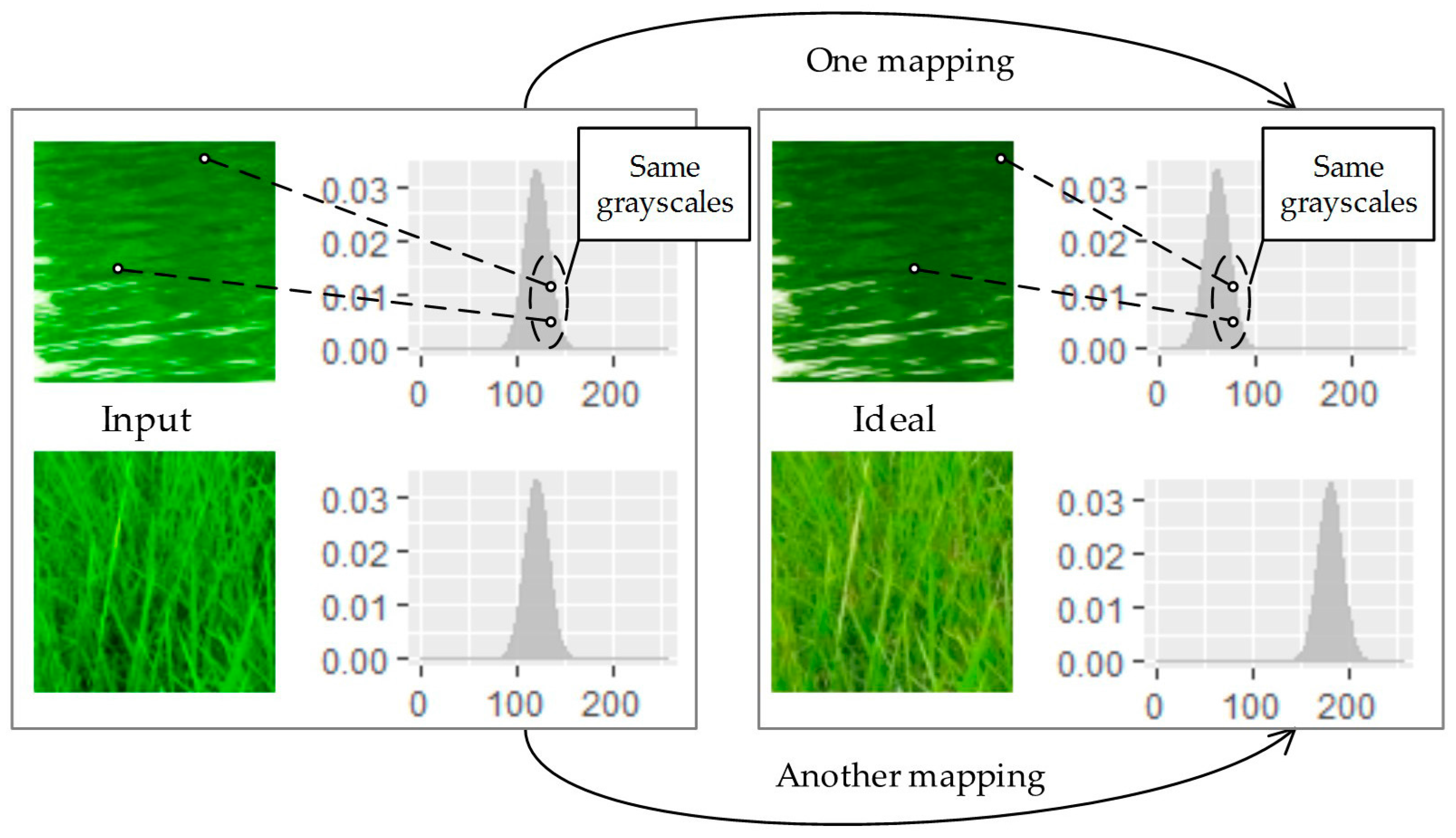
Scheme A is the case when both the input and reference are histograms, and this is essentially histogram matching. Many previous studies employ this scheme for simplicity, for example, histogram matching and low order statistics matching in various color spaces. Since histograms do not contain the content information, the corresponding histogram matching is not content related. Concretely speaking, two pixels that belong to two regions with different contents but with the same grayscale fall into the same bin of the histogram, and have to be assigned to the same grayscale value in the output image, which does not meet Property 3. In order for one distribution with different contexts to be correctly matched to different corresponding distributions, we cannot enclose different transformations in one unified mapping (see Figure 2). This should not be appropriate for large scale datasets that demand a high degree of automation.
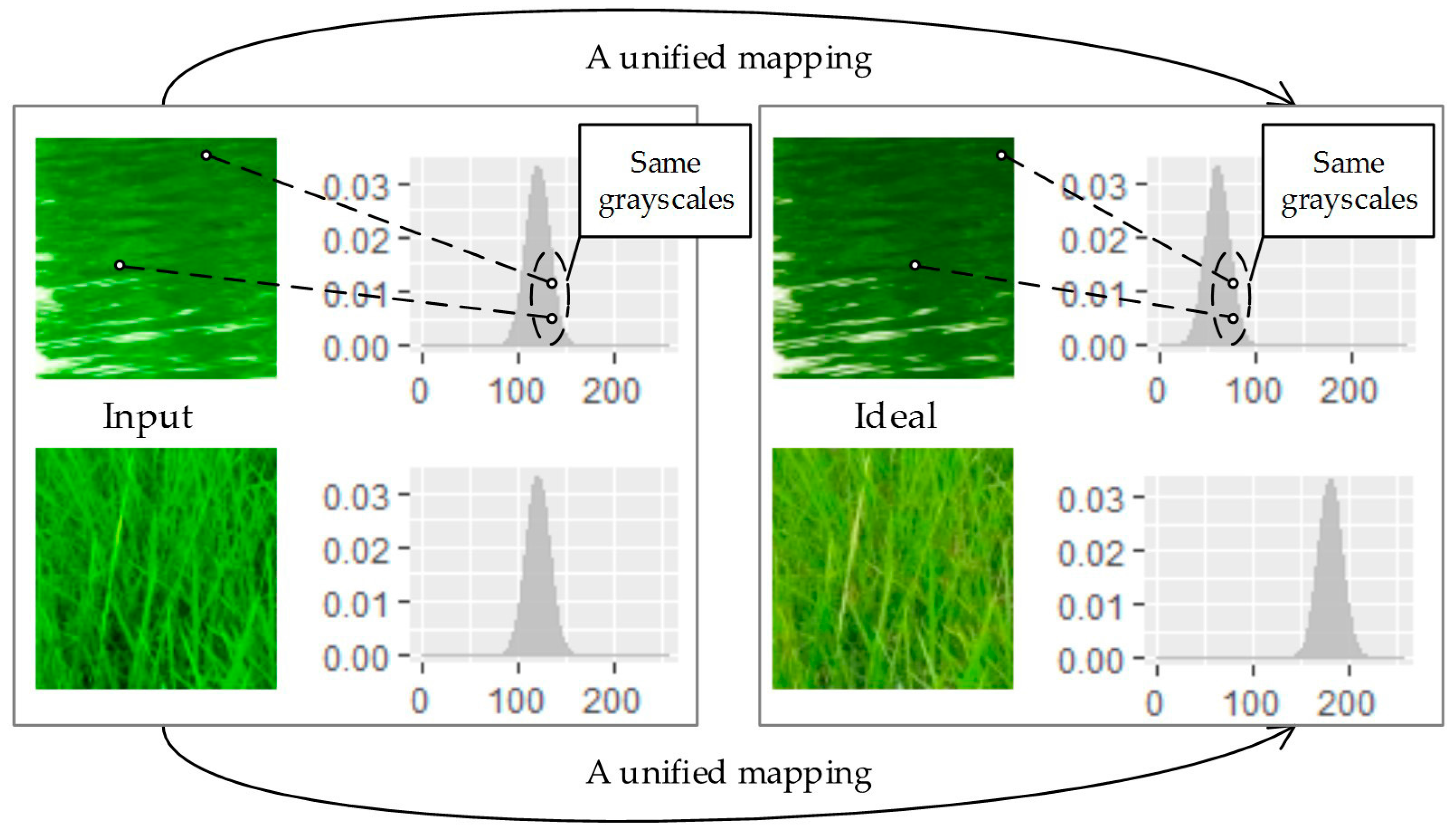
Scheme B corresponds to the case where both the input and output are images, which is usually referred to as image to image translation. The image certainly contains much more information than its histogram, thus providing a possibility that the mapping is content related. Although Property 3 can be satisfied, this scheme emphasizes the content of the image, and the consequence is that the pixels with same grayscales may be mapped to different grayscales as their contexts could be different, and in this case Property 1 is violated (see Figure 3).
Scheme C is the case where the input is an image and the output is a histogram. As mentioned above, scheme A does not satisfy Property 3 because the context of the image is not used, while scheme B violates Property 1. Mapping one image to another, with constraints that the pixels with the same grayscales also have the same grayscale values in the output, is essentially a grayscale to grayscale transforming process. Under such circumstances, the output of scheme B is always equivalent to that of scheme C. Since scheme C automatically possesses Properties 1 and 3, the task has been now converted to devise the algorithm so that it possesses Property 2 as well (see Figure 4). The task is addressed under an optimal transporting framework, which will be elaborated in Section 2.2.
The scheme of type D corresponds to the case where the input is the histogram and the output is the image. Since it is nearly impossible to determine a transformation mapping of a histogram to an image, we do not take this case into consideration.
2.2. Optimal Transporting Perspective of View
Denote u and v as the input and the reference color distributions, then is a mapping that transforms u to v. The total cost of can be defined as [25,26,27]:
where is the cost of transporting one unit of mass from x to y, and is the joint probability measure of , having u and v as its marginal distributions. Again, indicates the number of color channels and is the collection of every feasible .
Finding the transformation that minimizes the total cost is known as the Monge’s optimal transportation problem, or the MK problem. The solution to the problem is the gradient of some convex function [25,27,28]:
Specifically in one dimensional cases, this statement is equivalent to monotonicity, as consequence meets Property 2.
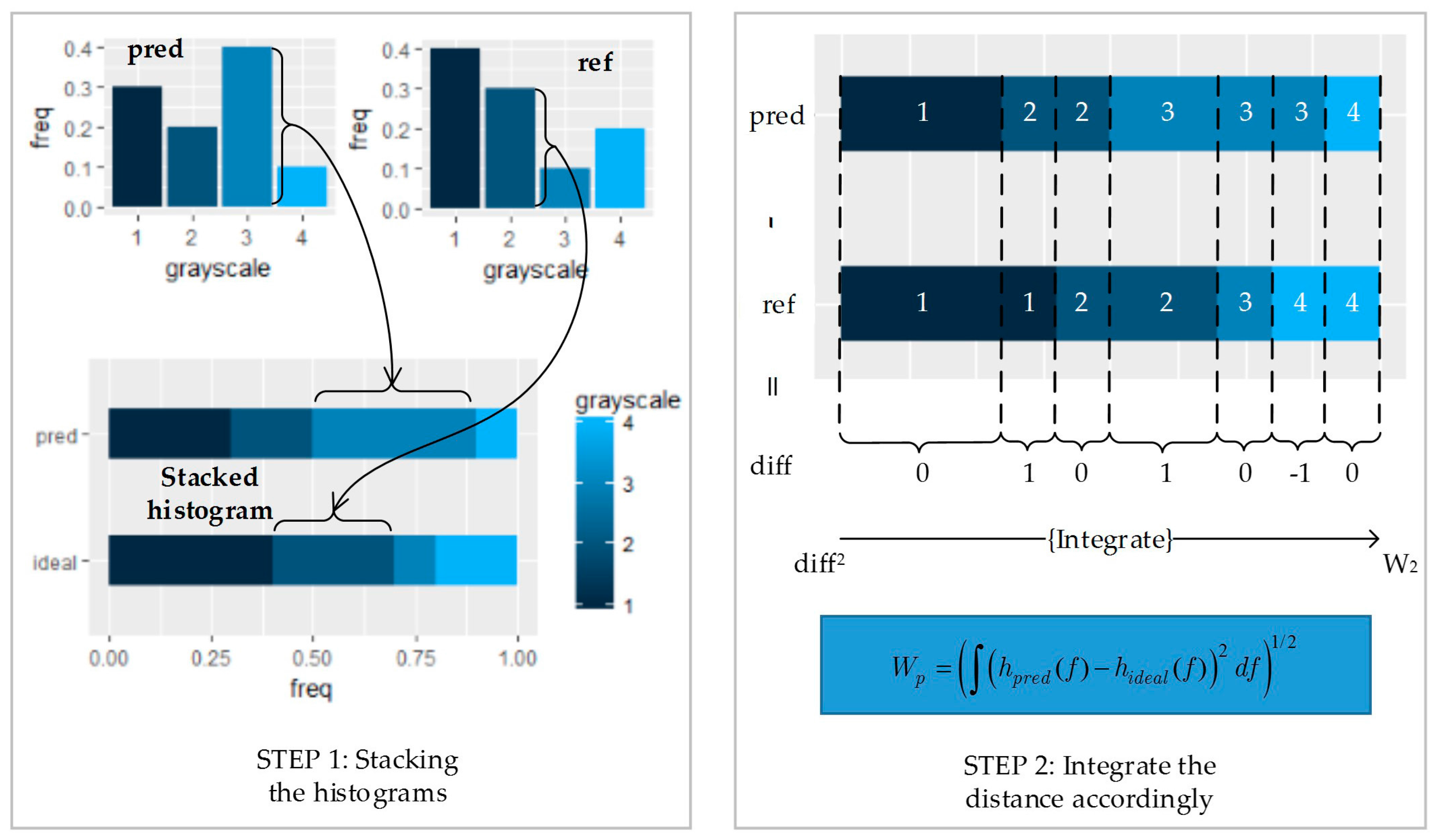
For high dimensional problems, the solution of the MK problem is intractable. In this paper, the distributions of the channels are matched separately. The Wasserstein distance between the inferred values and the ideal values can be calculated in the following way: first sort the pixels on a 1-D axis, and then calculate the distance between each pair of inferred pixels and the ideal pixels accordingly. This is equivalent to using a stacked histogram (see Figure 5). The Wasserstein distance when p equals 2 can be formulated as:
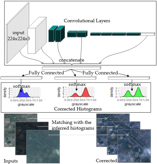
2.3. The Model Structure
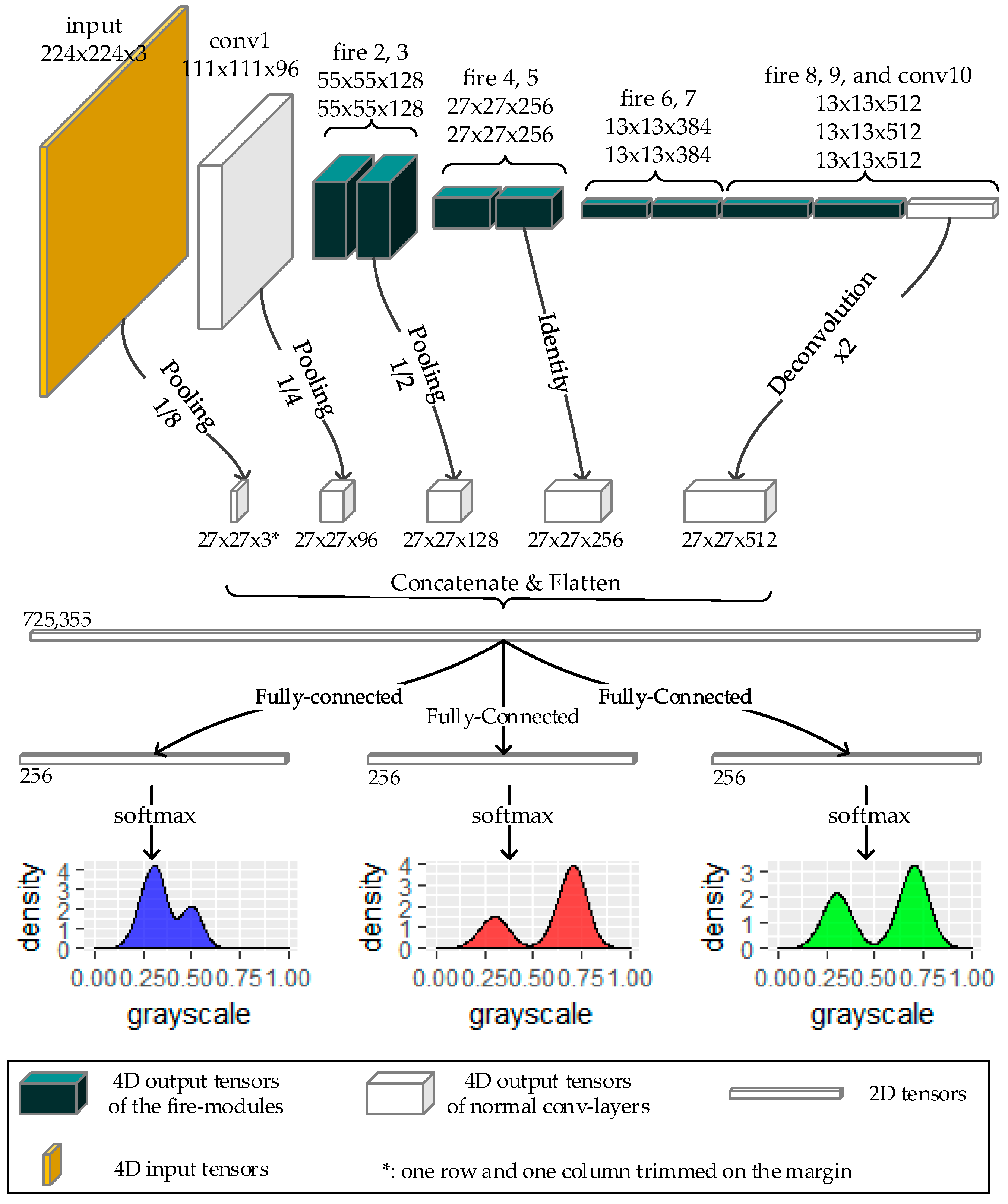
The transformation can be fitted by a CNN model, where the Wasserstein distance plays the role of the loss function. To reduce the memory and computation burden, we used a modified version of Squeeze-net v1.1 [29] (see Figure 6 and Figure 7). In this section we will first introduce the basic modules and then go on to state the major modifications.
2.3.1. Basic Modules
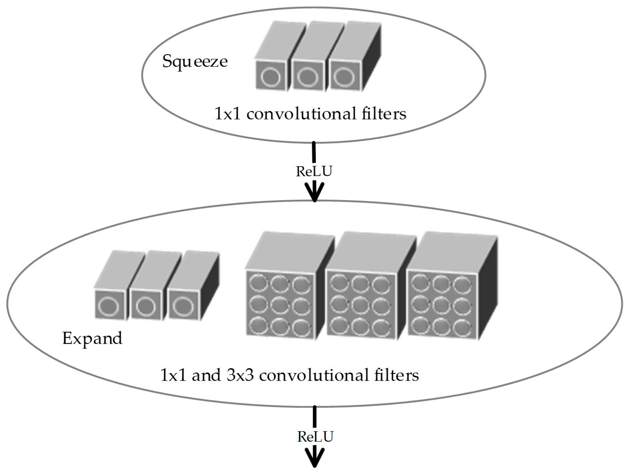
The Squeeze-net is a light-weight convolutional neural network. The basic modules of the squeeze-net are called the “fire” modules [29], and each consists of two convolution layers, the “squeeze” layer and the “expand” layer. The kernels in the “squeeze” layers are all of 1 × 1 sizes to maximally lessen the parameters inside the model and reduce the computational burden. Two types of kernels, 1 × 1 and 3 × 3 filters, comprise the “expand” layer. The “fire” modules prove to be computationally efficient, and also make the network less likely to be over fitted, as it “squeezes” the amount of parameters to a much smaller scale. In our experiment, the final global average pooling layer and the softmax layer of the squeeze-net was removed, and the rest of the parts were used to extract the features from the raw input images.
2.3.2. The Multi-Scale Concatenation and the Histogram Predictors
As stated in Section 2.3.1, we used a modified version of Squeeze-net to extract features from the input images. The layers at different levels in the CNN model extract features at different scales, and each level has its own characteristics. In general, the former layers in the CNN model are more associated with the raw pixels, while the latter ones are more meaningful in semantic senses [30,31]. Besides, the scales of the former feature maps are also different from the latter ones.
To utilize the information from different scales and semantic levels, we used a concatenating structure. In order for the feature maps to be concatenated, average pooling and deconvolution operations were applied to resize them to a unified shape (27 × 27). All the padding modes in the pooling layers were “valid”, so that the residual parts which could not fill up the pooling kernel were discarded. The strides and kernel sizes within each pooling layer were the same. All the resized shapes were 27 × 27, except for the input, whose output was 28 × 28. Its last row and column were trimmed in order to be consistent with the other tensors to be concatenated. The concatenated feature maps were then flattened into a 2-dimensional tensor of 725,355 length, and then was fed into three fully-connected layers separately, one for each channel (blue, green, and red). The fully-connected layer was then attached by a softmax head each to infer the corrected color distribution.
2.4. Data Augmentation
Data augmentation was performed on the original inputs to avoid over fitting as well as to enclose more patterns of color discrepancy into the model. The augmentation operations include:
- Random cropping: A patch of 227 × 227 is cropped at a random position from each 256 × 256 sample. It is worth noting that this implies that no registration is needed in the training process.
- Random flipping: Each sample in the input batch is randomly horizontally and vertically flipped by a chance of 50%.
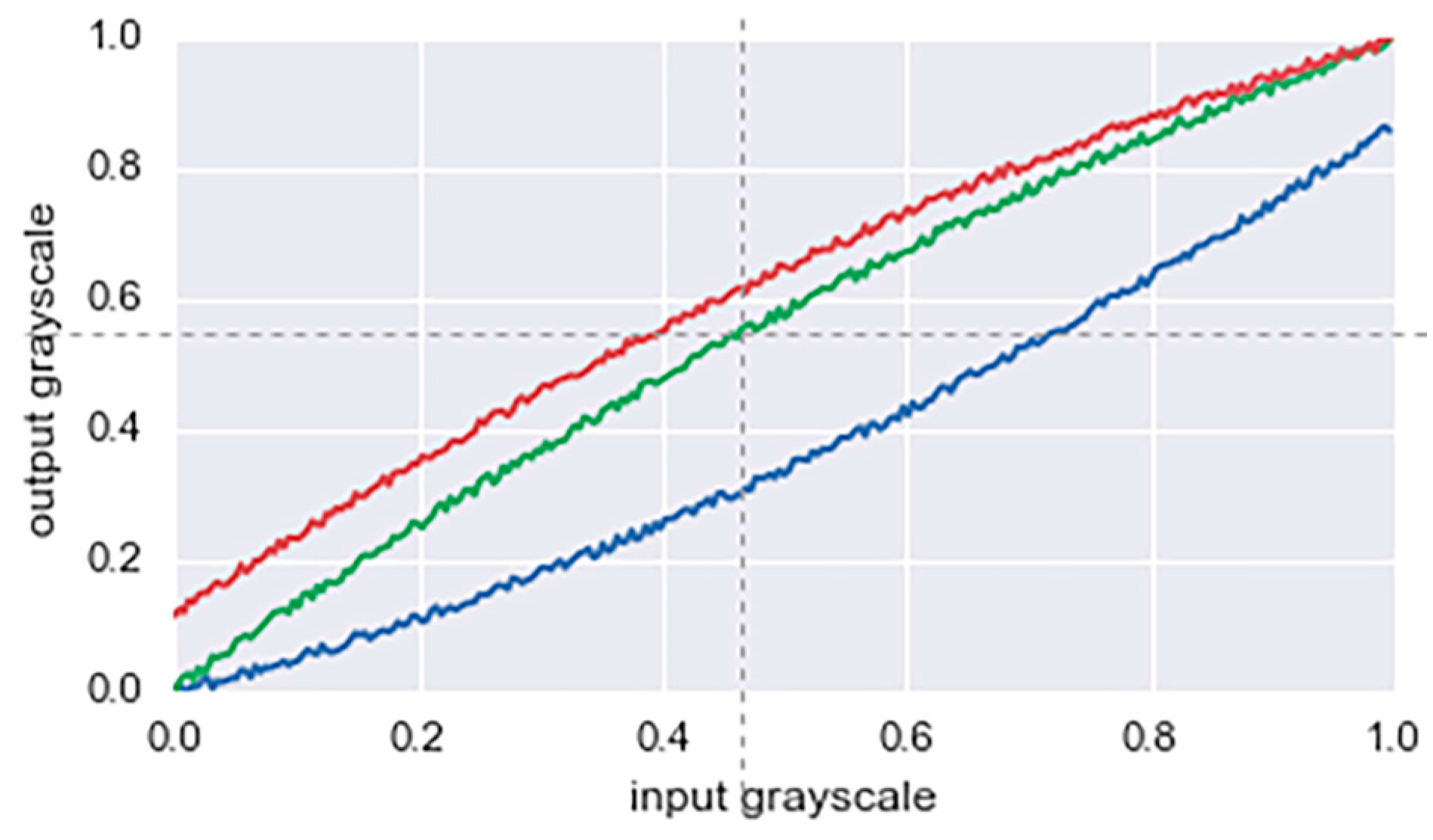
- Random color augmentation: The brightness, saturation, and gamma values of the input color are randomly shifted. Small perturbations are added to each color channel. Figure 8 shows an example of such transformation of the color distribution.
2.5. Algorithm Flow Chart
The entire model can be trained in an end-to-end fashion with the gradient descent algorithm, as displayed in Algorithm 1 ( Algorithm flow of the training process).
| Algorithm 1. Training Process of the Automatic Color Matching WCNN, Our Proposed Algorithm. |
| Notations: , the parameters in the WCNN model; , the gradients w.r.t. ; , the predicted color distribution; , the reference color distribution; , the Wasserstein loss. Required constants: , the learning rate; m, the batch size. Required initial values: , the initial parameters. 1: while has not converged do 2: Sample a batch from the input data 3: Sample a batch from the reference data 4: Apply random augmentation to 5: ← 6: ← 7: end while |
3. Results
We had our algorithm evaluated with satellite images from GF1 and GF2 that cover the same areas. The GF2 images were chosen as the reference. The parameters of the data are listed in Table 2.
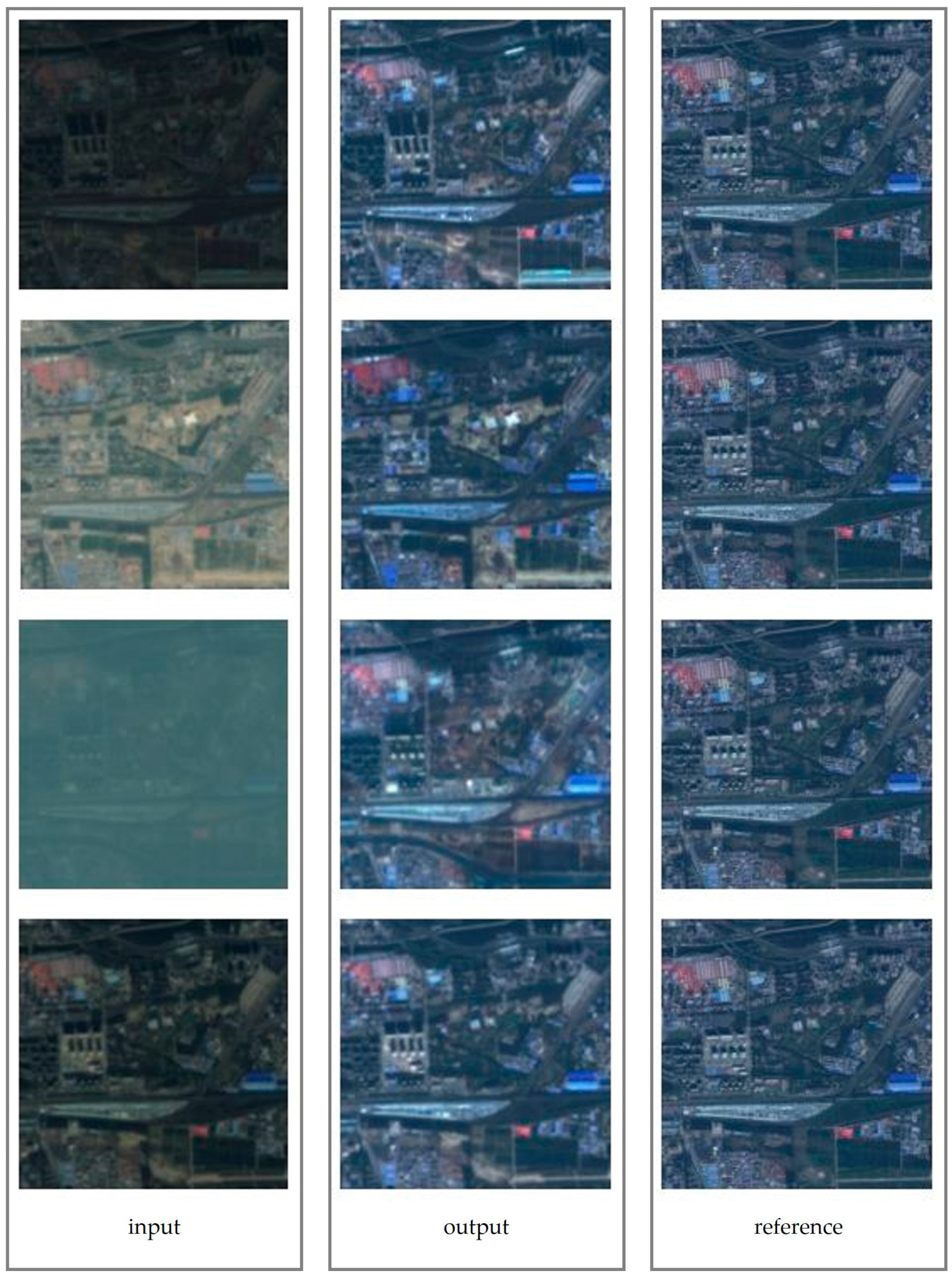
The direct outputs of WCNN are the inferred distributions (or histograms, see Figure 9) based on the contents of the input images. The corrected images are obtained by histogram matching (see Figure 10). The reference images are only used in the training process and are unnecessary in practical applications, as the purpose of the WCNN model is to generate the reference histogram when there are no available ones. It is worth noting that the patches were only roughly sliced according to the longitude and the latitude information within the GeoTIFF files, so registration was not necessary, and neither was pre-segmentation.
4. Discussion
4.1. Comparison between KL Divergence and Wasserstein Distance
As has been mentioned in Section 2.2, the Wasserstein distance is a natural choice to represent the difference between two color distributions. The Kullback–Leibler divergence (also known as KL divergence) is another commonly used measure (but not a metric) in such circumstances. The definition of KL divergence [27] is:
and the definition of 2-Wasserstein distance is:
Consider two simple distributions, and , as shown in Figure 11. The Kullback–Leibler divergence should be:
And the Wasserstein distance is:
Because both the Wasserstein metric and the KL divergence are fully differentiable, there is no difference in the back-propagation pipeline between the two losses. From the above discussion, however, we could see that the Wasserstein distance is more numerically stable compared to the KL divergence.
4.2. Connection and Comparison with Other Color Matching Methods
Histogram matching can be regarded as the simplest case of color matching. It is widely used in seamless mosaic workflows. The method requires that a reference image is selected for each input, which certainly puts restriction on the applications with large scale datasets. Wasserstein CNN is able to directly predict the corrected color distribution, and the histogram matching is the final step in the workflow of our proposed method (but not the only choice, other sample-based color matching methods would also do).
Matching low order statistics faces similar problems. Its performance is closely related to the similarity between the input images and the reference images. To handle low similarity cases, the images may have to be segmented and the color needs to be transferred part to part. Besides, for images with complex contents, color leakage on the edges could be a problem, and the image quality will degrade. Considering these restrictions, such methods may not be appropriate for automatic color matching in remote sensing applications. Matching the exact distribution is more precise than just matching the low order statistics, but is also more complex and computationally expensive. To match two non-Gaussian distributions, iterative approaches have to be exploited, as there are no closed-form solutions [8]. The Wasserstein CNN method is non-iterative, and is more suitable for large scale processing.
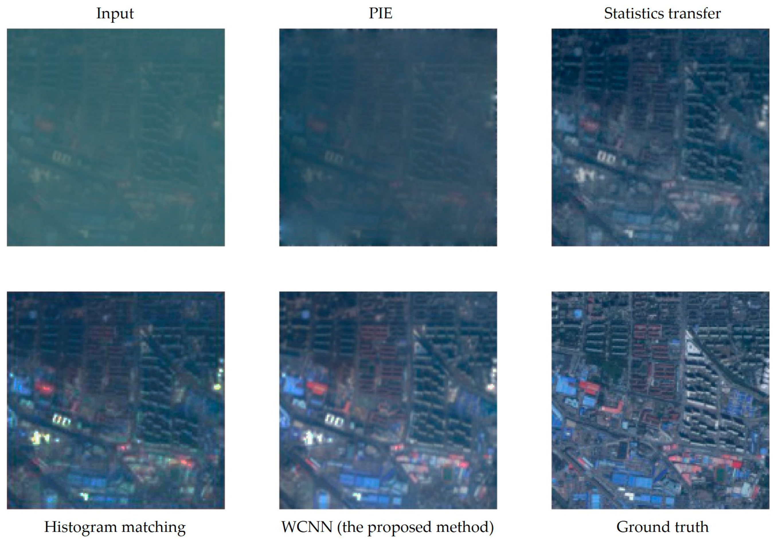
Poisson image editing (PIE) is another well-known color matching method. Rather than directly matching the color distributions, the PIE method tries to preserve the gradients of the input image and matches the pixel values on the border to those in the reference image. The problem is equivalent to solving a Poisson equation. However, in our case, this idea might not be very appropriate, because the gradients between the input image and the reference image can be very different, especially when the atmosphere visibility is low (see the PIE result in Figure 12).
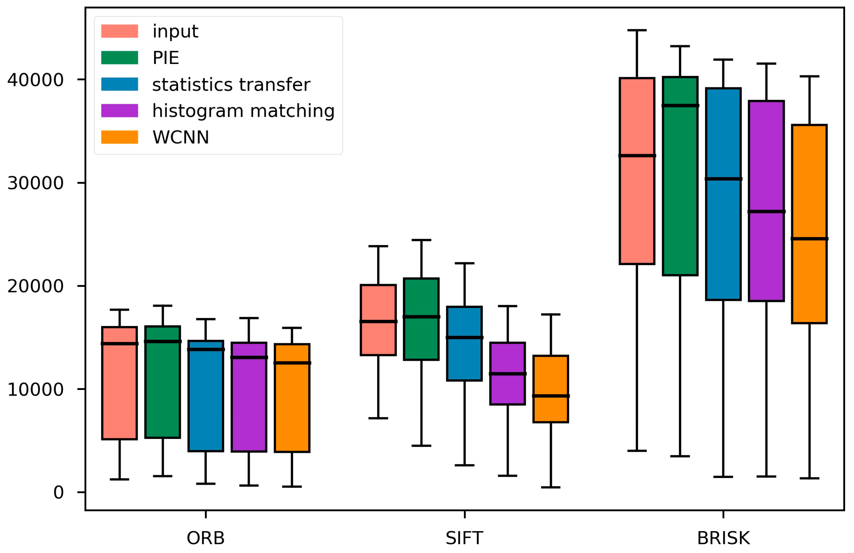
Comparisons between the color matching methods are displayed in Figure 12. The ground truth was not included in the training set, as it was supposed as an unknown in the color matching problem. Because the PIE, statistics transferring, and the histogram matching methods are all sample-based, an image must be selected from the training set to act as the reference. However, all that the WCNN model needs is the input image, thus it can operate without selecting such a reference. As the reference is not likely to be exactly the same as the ground truth, we can see the color discrepancy between the output and the ground truth in the results of PIE, statistics transferring, and histogram matching in Figure 12. Also, several features and descriptors were computed for all input images, output images, and the ground truth images in the test set, including the Oriented FAST and Rotated BRIEF (ORB) descriptor, the Scale-Invariant Feature Transform (SIFT) descriptor, and the Binary Robust Invariant Scalable Keypoints (BRISK) descriptor. To be a representation of similarity, the distances between the features of the output and the ground truth are computed, and are displayed in the boxplots in Figure 13.
From Figure 13 we can see that generally the processed images are closer to the ground truth, in regards to the distances of the feature descriptors, except for the PIE method. One of the reasons why PIE fails to generate high quality results is that the low atmosphere visibility may deteriorate the gradients, resulting in a significant difference between the gradients of the input image and the ground truth. The WCNN model results achieve the maximum similarity to the ground truth, and the model is also the most stable one.
4.3. Processing Time and Memory Comsumption
The processing time of 512 patches with a size of 227 × 227 × 3 on a single NVIDIA® GeForce® GTX 1080 graphics processing unit is 0.408 s, or s for a single patch, which means that the method could handle images as large as 2000 × 2000 in real time. A total of 6990 MB memory is consumed for 512 patches, or 13.7 MB for each.
5. Conclusions
This paper presents a nonparametric color correcting scheme in a probabilistic optimal transport framework, based on the Wasserstein CNN model. The multi-scale features are first to be extracted from the intermediate layers, and then are used to infer the corrected color distribution which minimizes the errors with respect to the ground truth. The experimental results demonstrate that the method is able to handle images of different sources, resolutions, and illumination and atmosphere conditions. With high efficiency in computing speed and memory consumption, the proposed method shows its prospects for utilization in real time processing of large-scale remote sensing datasets.
We are currently extending the global color matching algorithm to take the local inhomogeneity of illumination into consideration, in order to enhance the precision. Local histogram matching of each band could serve for reflectance retrieval and atmospheric parameter retrieval purposes, and the preliminary results are encouraging.
Acknowledgments
This work was supported by the National Natural Science Foundation of China (Grant No. 61331017.)
Author Contributions
Jiayi Guo and Bin Lei conceived and designed the experiments; Jiayi Guo performed the experiments; Jiayi Guo analyzed the data; Bin Lei and Chibiao Ding contributed materials and computing resources; Jiayi Guo and Zongxu Pan wrote the paper.
Conflicts of Interest
The authors declare no conflict of interest.
References
- Haichao, L.; Shengyong, H.; Qi, Z. Fast seamless mosaic algorithm for multiple remote sensing images. Infrared Laser Eng. 2011, 40, 1381–1386. [Google Scholar]
- Rau, J.; Chen, N.-Y.; Chen, L.-C. True orthophoto generation of built-up areas using multi-view images. Photogramm. Eng. Remote Sens. 2002, 68, 581–588. [Google Scholar]
- Reinhard, E.; Adhikhmin, M.; Gooch, B.; Shirley, P. Color transfer between images. IEEE Comput. Graph. Appl. 2001, 21, 34–41. [Google Scholar] [CrossRef]
- Abadpour, A.; Kasaei, S. A fast and efficient fuzzy color transfer method. In Proceedings of the IEEE Fourth International Symposium on Signal Processing and Information Technology, Rome, Italy, 18–21 Dcember 2004; pp. 491–494. [Google Scholar]
- Kotera, H. A scene-referred color transfer for pleasant imaging on display. In Proceedings of the IEEE International Conference on Image Processing, Genova, Italy, 14 November 2005. [Google Scholar]
- Morovic, J.; Sun, P.-L. Accurate 3d image colour histogram transformation. Pattern Recognit. Lett. 2003, 24, 1725–1735. [Google Scholar] [CrossRef]
- Neumann, L.; Neumann, A. Color style transfer techniques using hue, lightness and saturation histogram matching. In Proceedings of the Computational Aesthetics in Graphics, Visualization and Imaging, Girona, Spain, 18–20 May 2005; pp. 111–122. [Google Scholar]
- Pitie, F.; Kokaram, A.C.; Dahyot, R. N-dimensional probability density function transfer and its application to color transfer. In Proceedings of the Tenth IEEE International Conference on Computer Vision, Beijing, China, 17–21 October 2005; pp. 1434–1439. [Google Scholar]
- Reinhard, E.; Pouli, T. Colour spaces for colour transfer. In Proceedings of the International Workshop on Computational Color Imaging, Milan, Italy, 20–21 April 2011; Springer: Berlin/Heidelberg, Germany; pp. 1–15. [Google Scholar]
- An, X.; Pellacini, F. User-controllable color transfer. In Computer Graphics Forum; Wiley Online Library: Hoboken, NJ, USA, 2010; pp. 263–271. [Google Scholar]
- Pouli, T.; Reinhard, E. Progressive color transfer for images of arbitrary dynamic range. Comput. Graph. 2011, 35, 67–80. [Google Scholar] [CrossRef]
- Tai, Y.-W.; Jia, J.; Tang, C.-K. Local color transfer via probabilistic segmentation by expectation-maximization. In Proceedings of the IEEE Computer Society Conference on Computer Vision and Pattern Recognition, San Diego, CA, USA, 20–26 June 2005; pp. 747–754. [Google Scholar]
- HaCohen, Y.; Shechtman, E.; Goldman, D.B.; Lischinski, D. Non-rigid dense correspondence with applications for image enhancement. ACM Trans. Graph. 2011, 30, 70. [Google Scholar] [CrossRef]
- Kagarlitsky, S.; Moses, Y.; Hel-Or, Y. Piecewise-consistent color mappings of images acquired under various conditions. In Proceedings of the IEEE 12th International Conference on Computer Vision, Kyoto, Japan, 29 September–2 October 2009; pp. 2311–2318. [Google Scholar]
- Bonneel, N.; Sunkavalli, K.; Paris, S.; Pfister, H. Example-based video color grading. ACM Trans. Graph. 2013, 32, 39:1–39:12. [Google Scholar] [CrossRef]
- Wang, Q.; Yan, P.; Yuan, Y.; Li, X. Robust color correction in stereo vision. In Proceedings of the 2011 18th IEEE International Conference on Image Processing, Brussels, Belgium, 11–14 September 2011; pp. 965–968. [Google Scholar]
- Gong, H.; Finlayson, G.D.; Fisher, R.B. Recoding color transfer as a color homography. arXiv, 2016; arXiv:1608.01505. [Google Scholar]
- Liao, D.; Qian, Y.; Li, Z.-N. Semisupervised manifold learning for color transfer between multiview images. In Proceedings of the 2016 23rd International Conference on Pattern Recognition, Cancun, Mexico, 4–8 December 2016; pp. 259–264. [Google Scholar]
- Isola, P.; Zhu, J.-Y.; Zhou, T.; Efros, A.A. Image-to-image translation with conditional adversarial networks. arXiv, 2016; arXiv:1611.07004. [Google Scholar]
- Larsson, G.; Maire, M.; Shakhnarovich, G. Learning representations for automatic colorization. In Proceedings of the European Conference on Computer Vision, Amsterdam, The Netherlands, 8–16 October 2016; pp. 577–593. [Google Scholar]
- Zhang, R.; Isola, P.; Efros, A.A. Colorful image colorization. In Proceedings of the European Conference on Computer Vision, Amsterdam, The Netherlands, 8–16 October 2016; pp. 649–666. [Google Scholar]
- Wang, Q.; Lin, J.; Yuan, Y. Salient band selection for hyperspectral image classification via manifold ranking. IEEE Trans. Neural Netw. Learn. Syst. 2016, 27, 1279–1289. [Google Scholar] [CrossRef] [PubMed]
- Vallet, B.; Lelégard, L. Partial iterates for symmetrizing non-parametric color correction. ISPRS J. Photogramm. Remote Sens. 2013, 82, 93–101. [Google Scholar] [CrossRef]
- Danila, B.; Yu, Y.; Marsh, J.A.; Bassler, K.E. Optimal transport on complex networks. Phys. Rev. E Stat. Nomlin. Soft. Matter Phys. 2006, 74, 046106. [Google Scholar] [CrossRef] [PubMed]
- Villani, C. Optimal Transport: Old and New; Springer: Berlin, Germany, 2008. [Google Scholar]
- Pitié, F.; Kokaram, A. The linear monge-kantorovitch linear colour mapping for example-based colour transfer. In Proceedings of the European Conference on Visual Media Production, London, UK, 27–28 November 2007. [Google Scholar]
- Frogner, C.; Zhang, C.; Mobahi, H.; Araya, M.; Poggio, T.A. Learning with a wasserstein loss. In Proceedings of the Advances in Neural Information Processing Systems, Montreal, QC, Canada, 2015; pp. 2053–2061. [Google Scholar]
- Cuturi, M.; Avis, D. Ground metric learning. J. Mach. Learn. Res. 2014, 15, 533–564. [Google Scholar]
- Iandola, F.N.; Han, S.; Moskewicz, M.W.; Ashraf, K.; Dally, W.J.; Keutzer, K. Squeezenet: Alexnet-level accuracy with 50x fewer parameters and <0.5 mb model size. arXiv, 2016; arXiv:1602.07360. [Google Scholar]
- Long, J.; Shelhamer, E.; Darrell, T. Fully convolutional networks for semantic segmentation. In Proceedings of the IEEE Conference on Computer Vision and Pattern Recognition, Boston, MA, USA, 2015; pp. 3431–3440. [Google Scholar]
- Chen, L.-C.; Papandreou, G.; Kokkinos, I.; Murphy, K.; Yuille, A.L. Semantic image segmentation with deep convolutional nets and fully connected crfs. arXiv, 2014; arXiv:1412.7062. [Google Scholar]
Figure 1.
Color discrepancy in remote sensing images. (a,b) Digital Globe images on different dates from Google Earth; (c,d) Digital Globe (bottom, right) and NASA (National Aeronautics and Space Administration) Copernicus (top, left) images on the same date from Google Earth; (e) GF1 (Gaofen-1) images from different sensors, same area and date.

Figure 2.
Matching algorithms of “scheme A” take both input and reference in the form of histograms. As this scheme is not content related, two similar distributions with different contexts could be not be mapped to their corresponding reference with one unified mapping.
Figure 2.
Matching algorithms of “scheme A” take both input and reference in the form of histograms. As this scheme is not content related, two similar distributions with different contexts could be not be mapped to their corresponding reference with one unified mapping.

Figure 3.
Matching algorithms of “scheme B” take both input and reference in the form of images. Similar distributions could be mapped to different corresponding references, as the scheme is content based. However, the same grayscales could be mapped to different grayscales when they are in different contexts, violating Property 1.

Figure 4.
Matching algorithms of “scheme C” take images as inputs and histograms as references in the form of images. Similar distributions could be mapped to different corresponding references, as the scheme is content related.
Figure 4.
Matching algorithms of “scheme C” take images as inputs and histograms as references in the form of images. Similar distributions could be mapped to different corresponding references, as the scheme is content related.

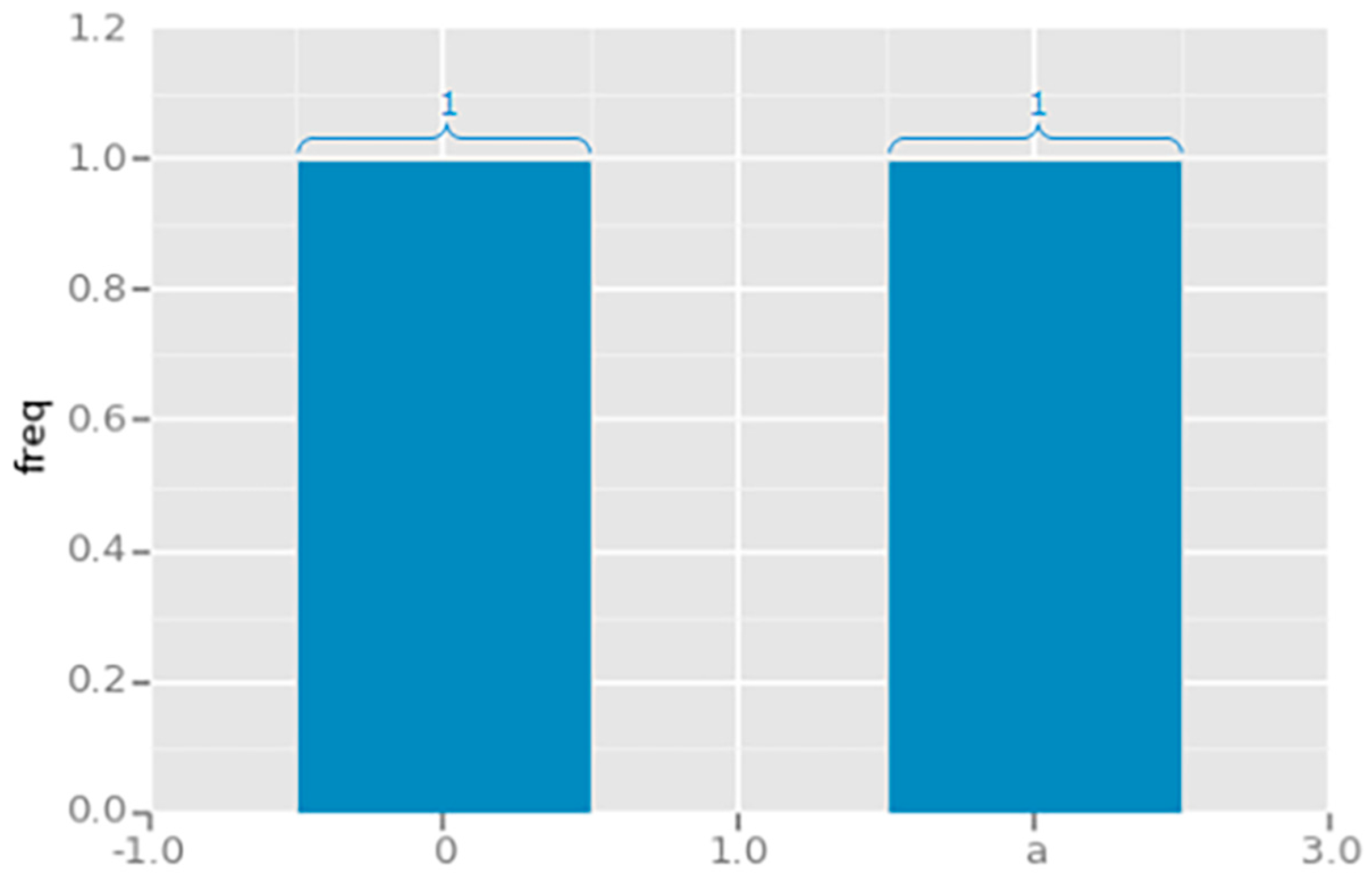
Figure 5.
Calculation method of the Wasserstein distance between the inferred histograms and the ground-truth reference. STEP 1: stack the histograms on the frequency axis; STEP 2: subtract the stacked histograms, and integrate with respect to the cumulative frequency.
Figure 5.
Calculation method of the Wasserstein distance between the inferred histograms and the ground-truth reference. STEP 1: stack the histograms on the frequency axis; STEP 2: subtract the stacked histograms, and integrate with respect to the cumulative frequency.

Figure 6.
Structure of the “fire module” in the Squeeze-net.

Figure 7.
Model structure of the proposed model.

Figure 8.
Color transforming curves in the random augmentation process.

Figure 9.
Results of matching the color palette of GF1 to GF2. Bars: histograms of input patches; solid lines with color: predicted histograms of our model; dashed lines in black: histograms of reference images; from top to bottom: histograms of images of the same area, but under different illumination and atmospheric conditions.

Figure 10.
Color matching results of GF1 and GF2. From top to bottom: satellite images of the same area, but under different illumination and atmospheric conditions; left: input images; middle: output images with the predicted color palette; right: reference images, only needed in the training process to calculate the loss function. The model is able to infer the corrected color palette based on the content of the input images in the absence of a reference, when the model is fully trained.

Figure 11.
Two one-dimensional uniform distributions.

Figure 12.
Comparisons between color matching methods.

Figure 13.
Boxplots of L1-norm distances between the processed images and the ground truth with respect to left: ORB; middle: SIFT, and right: BRISK feature descriptors. The distances represent the dissimilarity between the processed results and the ground truth (the smaller the better). There are five horizontal line segments in each patch, indicating five percentiles of the distances within the processed images by the corresponding method; from top to bottom: the maximum (worst) distance, the worst-25% distance, the median distance, the best-25% distance, and the minimum (best) distance.


Table 1.
Different color matching schemes according to the input form and the reference form.
| Input | Reference | Scheme |
|---|---|---|
| Histogram | Histogram | A |
| Image | Image | B |
| Image | Histogram | C |
| Histogram | Image | D |
Table 2.
Parameters of the GF1 and GF2 data in the experiment.
| Resolution | GF1 | GF2 |
|---|---|---|
| 8 m | 4 m | |
| Band1 | 0.45–0.52 μm | 0.45–0.52 μm |
| Band2 | 0.52–0.59 μm | 0.52–0.59 μm |
| Band3 | 0.63–0.69 μm | 0.63–0.69 μm |
© 2017 by the authors. Licensee MDPI, Basel, Switzerland. This article is an open access article distributed under the terms and conditions of the Creative Commons Attribution (CC BY) license (http://creativecommons.org/licenses/by/4.0/).
Share and Cite
MDPI and ACS Style
Guo, J.; Pan, Z.; Lei, B.; Ding, C. Automatic Color Correction for Multisource Remote Sensing Images with Wasserstein CNN. Remote Sens. 2017, 9, 483. https://0-doi-org.brum.beds.ac.uk/10.3390/rs9050483
AMA Style
Guo J, Pan Z, Lei B, Ding C. Automatic Color Correction for Multisource Remote Sensing Images with Wasserstein CNN. Remote Sensing. 2017; 9(5):483. https://0-doi-org.brum.beds.ac.uk/10.3390/rs9050483
Chicago/Turabian StyleGuo, Jiayi, Zongxu Pan, Bin Lei, and Chibiao Ding. 2017. "Automatic Color Correction for Multisource Remote Sensing Images with Wasserstein CNN" Remote Sensing 9, no. 5: 483. https://0-doi-org.brum.beds.ac.uk/10.3390/rs9050483
Note that from the first issue of 2016, this journal uses article numbers instead of page numbers. See further details here.