
Multi-Scale Analysis of Very High Resolution Satellite Images Using Unsupervised Techniques


1
LISITE Laboratory, RDI Team–Institut Supérieur d’Électronique de Paris, 10 rue de Vanves, 92130 Issy Les Moulineaux, France
2
CNRS UMR 7030 LIPN–Université Paris 13, Sorbonne Paris Cité, 99 av. J-B Clément, 93430 Villetaneuse, France
3
CNRS UMR 7357 ICube–Université de Strasbourg, 300 bd Sébastien Brant-CS 10413, F-67412 Illkirch CEDEX, France
4
CNRS UMR 7362 LIVE–Université de Strasbourg, 3 rue de l’Argonne, 67000 Strasbourg, France
*
Author to whom correspondence should be addressed.
Remote Sens. 2017, 9(5), 495; https://0-doi-org.brum.beds.ac.uk/10.3390/rs9050495
Submission received: 15 March 2017
/
Revised: 25 April 2017
/
Accepted: 12 May 2017
/
Published: 18 May 2017
(This article belongs to the Special Issue Learning to Understand Remote Sensing Images)
Abstract
:This article is concerned with the use of unsupervised methods to process very high resolution satellite images with minimal or little human intervention. In a context where more and more complex and very high resolution satellite images are available, it has become increasingly difficult to propose learning sets for supervised algorithms to process such data and even more complicated to process them manually. Within this context, in this article we propose a fully unsupervised step by step method to process very high resolution images, making it possible to link clusters to the land cover classes of interest. For each step, we discuss the various challenges and state of the art algorithms to make the full process as efficient as possible. In particular, one of the main contributions of this article comes in the form of a multi-scale analysis clustering algorithm that we use during the processing of the image segments. Our proposed methods are tested on a very high resolution image (Pléiades) of the urban area around the French city of Strasbourg and show relevant results at each step of the process.
1. Introduction
The recent advances of remote sensing technologies for Earth observation have led to a surge in the number of large and complex available data to process. For example, very high spatial resolution (VHR) satellite images covering large areas are nowadays commonly delivered by remote sensors (Pléiades, Worldview, Quickbird, Ikonos). The manual analysis of such images by experts to extract useful information would be overwhelming, and the use of machine learning techniques is more than ever necessary to obtain satisfactory results in a fair amount of time. However, the majority of popular machine learning techniques for classification purposes (known as supervised learning) also require human intervention in the sense that the computer can only learn to recognize things that have already been learned and identified by humans based on similar data. In the case of VHR images, since they have a high level of detail and deal with a wide variety of landscapes, such knowledge to feed the machine learning algorithm is quite often unavailable or incomplete.
Within this context, in this article, we propose a complete methodology for an almost fully-unsupervised analysis of VHR images requiring only minimal knowledge on the data and little human intervention. We will discuss the different steps and challenges of going from the raw satellite image to the final segmented and clustered image where the different elements of interest can be linked to expert classes. In particular, the main novelty of this work lies in the proposition of a clustering algorithm that can process image segments and find multi-scale clusters matching the different scales of interest that can be found on VHR images.
Furthermore, our algorithm also provides minimal semantic information that can be used to link the clusters to land cover classes. Unlike the majority of methods in the literature, our proposed model focuses on object-based image analysis (OBIA) rather than pixel-based analysis. Indeed, it makes more sense to focus on objects rather than pixels that have little semantic value when using very high resolution [1,2].
Works closely related to this article include other unsupervised algorithms that have been proposed recently to process datasets built from the segments of non-hyperspectral VHR images:
- In [3], the authors propose an unsupervised algorithm that provides some low level semantic information on the clusters. This algorithm is the base that we used for the multi-scale method proposed in the learning step of this article. The improvements that we bring include that our proposed method covers the segmentation step, while the original algorithm does not. Furthermore, this algorithm was designed to produce a non-hierarchical hard partition, whereas our method can find the object at several scales of interest and produces multi-scale hierarchical clusters.
- In [4], the authors also tackle image data acquired from image segments. The method they used is based on the self-organizing map (SOM) algorithm, a known unsupervised neural network used for dimension reduction. While this methods considers dimension reduction aspects that our proposed algorithm does not handle, it is also limited to the learning step and can only provide hard partitions computed at a single scale of interest.
The remainder of this article is organized as follows: In Section 2, we present the different steps involved in VHR image processing and discuss the various challenges and state of the art methods for each step. In Section 3, we introduce the material and methods that we use in our experiments. In particular, we give the details of the multi-scale clustering algorithm that we use to process our data. Section 4 shows our experimental results and features various discussions on the results. Finally, in Section 5, we give our conclusions on this work, as well as some perspective on future extensions.
2. State of the Art on Unsupervised VHR Images Processing
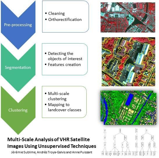
The fully-automated analysis of a satellite image can usually be decomposed into three steps: (1) a pre-processing step during which the image is prepared from raw sources (merging pictures, orthorectification, etc.); (2) a segmentation step that consists of grouping together adjacent pixels that are similar given a certain homogeneity criterion; these groups, called segments, should ideally be a good estimation of the geographical objects in the image [5,6]; (3) the segments created during Step 2 can then be fed to a supervised or unsupervised machine learning algorithm in order to recognize the elements in the image.
This succession of steps, all dependent on the previous ones, is summed up in Figure 1. As one can see, errors are quite likely to accumulate through the process.
In the next subsections, we will discuss the state of the art methods used during the segmentation and clustering step: we will go into detail on explaining which difficulties are encountered during each step and which techniques can be used to reduce the risk of error accumulation in order to ensure the best possible final results.
2.1. Image Segmentation
Image segmentation is the first critical step within the OBIA workflow and aims at finding segments that will correspond to the objects of interest in the image. Indeed, poor quality segments would likely lead to the computation of inaccurate and irrelevant descriptors, making the dataset difficult or even impossible to exploit by machine learning techniques in further steps.
A wide range of segmentation approaches and their ad hoc variants devoted to specific applications can be found in the literature. The reader interested in general segmentation approaches may refer to [7] for a complete survey on this topic.
In the context of remote sensing imaging, the most popular approaches are mainly these relying on region-based and spectral homogeneity paradigms. For instance, the mean-shift [8,9] applies a technique for estimating local modes in a multivariate distribution [10] to a joint spatial and spectral domain. For each pixel, local modes are computed with respect to a spectral and spatial similarity ranges so that in the end, each pixel is associated with the local mode’s spectral signature and the spatial location of its density probability distribution. Finally, pixels sharing the same local mode are merged together to generate the segments. Region-growing approaches, such as [11,12], are also commonly employed. They usually start by considering each pixel as a segment and then iteratively merge similar pixels based on a given homogeneity criterion. Other constraints such as a minimum or maximum segment size are often considered as well during the merging procedure. Other popular segmentation algorithms are based on the watershed transformation [13,14]. The main idea consists of considering the gradient image as a topographic surface. This surface is then flooded starting from the local minima of the image gradient. When two different flooding basins are about to merge, the process stops, and a watershed (segment boundary) is drawn. Finally, hierarchical strategies [15] are based on graph theory and consider the image (and the segments being created) as a tree structure in which lower level objects are close to the leafs and more abstract objects are at higher hierarchical levels. This structure allows focusing on objects at different levels of resolution or semantics.
While few efforts have been made in this area, evaluating the quality of a segmentation remains a key issue: image segmentation is an ill-posed problem, so almost any partition of the image can be considered as a correct segmentation given the general definition of image segmentation (i.e., partitioning the image by grouping similar pixels given a certain criterion). Thus, the definition of segmentation quality is usually dependent on a given application. In a remote sensing context, a perfect segmentation should map each segment to an object of interest in the image. Given this definition of quality, it is possible to distinguish mainly two kinds of segmentation errors: over-segmentation where objects are split into several segments; and under-segmentation where a single segment may contain several objects. There exist mainly three families of quality criteria:
- Subjective criteria, which basically rely on a visual examination of segmentation results. This task is long, tedious and does not provide an objective and quantitative evaluation.
- Supervised criteria [16,17], which consist of measuring the distance between one segmentation and a gold-standard segmentation. However, such a ground-truth generally has to be manually generated. Thus, it is very rare to dispose of complete reference datasets in remote sensing applications, making supervised metrics less reliable.
- Finally, unsupervised criteria [18], which consist of exploiting intrinsic segment and image properties. It is then necessary to accurately define and model the notion of quality without any external information. Many of these metrics rely on the number and size of segments [19], as well as statistics, such as band mean values or the standard deviation [17,20], or on local (per segment) quality estimation based on some homogeneity criterion in order to compute global quality metrics by aggregation of the local scores [21].
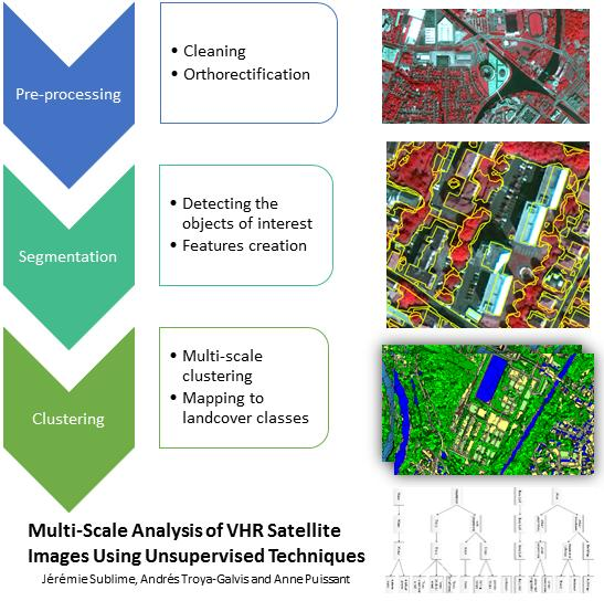
In short, segmentation algorithms should be used along with different quality metrics so that the produced segmentation has as few segmentation errors as possible. In practice, over-segmentation errors are usually tolerated as they can be easily corrected by further analysis; however, under-segmentation has to be avoided as much as possible, see Figure 2.
2.2. Unsupervised Analysis of the Segments
The objects extracted from an image during the segmentation can be seen as regular data, where each segment is described by several features from the original image, such as color attributes, as well as new features created during the segmentation process: surface of the segments, perimeter and elongation, shape information, color extrema, variance and average value of the attributes in the pixels of a given segment, texture information, contrast with the neighboring segments, etc.
Because the segments and their attributes can vary greatly depending on the image or the algorithm used for the segmentation process, it is very difficult to find similar data using the same attributes that could be used to train a supervised classifier to process such a segment-based dataset. Unsupervised methods are therefore most convenient to process such data acquired from a segmentation. In particular, clustering techniques that consist of finding groups of similar data in a dataset are usually a good choice since the clusters can be built without external knowledge and can usually be easily linked to expert-defined classes once they have been built. These methods are therefore popular for both object-based and pixel-based image analysis [22,23,24,25].
The main known weakness of unsupervised approaches for object identification in images is that there is no warranty that the clusters found by the algorithms will end up being pertinent classes. A first possible solution consists of using semi-supervised approaches instead of fully-unsupervised ones: In the case of pixel-based analysis of VHR images, a solution proposed in the literature is to guide the clustering process using ontologies [26,27], a tool commonly used in supervised process. The results achieved using these methods are promising, but seem limited to a very low number of clusters/classes. The second solution that is usually preferred in the context of OBIA is to use a mixed clustering and Markov random field (MRF) approach [28,29,30] with the goal of using all of the extra attributes from the segmentation in the clustering process (shapes, texture, contrast), but also to use the information from the neighborhood dependencies in order to influence the clustering of each segment based on both its characteristics and the cluster to which the neighboring segments belong. Other approaches have been attempted using topological clustering instead of MRF-based techniques [4] for OBIA.
One advantage of MRF-based approaches is that these methods are used for both segmentation, classification and clustering. In our case, we are particularly interested in the segmentation and clustering uses. Using MRF-based methods has the advantage that it can deal with over-segmented data just fine, thus reducing of error accumulation from the segmentation step during the clustering step. In the remainder of this section, we will focus on the MRF-based approach, as it will be the basis of our proposed method in the experiments.
The clustering task using MRF models can be seen as a graph partitioning problem, where each segment is a node of the graph and the edges are represented by the neighborhood dependencies between the segments. Assigning each segment to a cluster based on its features and its neighbors (see Figure 3) is indeed equivalent to finding the optimal cuts in the graph to separate dissimilar neighbor segments. This process will provide both the clusters and a new segmentation as a by-product.
There are many methods in the literature to solve this kind of problem: the graph-cut algorithm [31], the integer projected fixed point method [32], the graduated non-convexity and concavity procedure [33], the iterated conditional modes (ICM) [34] and hybrid algorithms mixing the principle of expectation-maximization and the ICM algorithm [35].
In the case of segments from VHR images, approaches with the lowest complexity are usually preferred due to the expected large size of the graph. To this end, an adaptation of the hybrid EM-ICM approach capable of assessing the affinities between neighbor segments of different pixel was proposed in the form of a semantic-rich ICM [3] (SR-ICM). This algorithm is similar to what already existed for semantic-rich pixel-based MRF models [36], but adapted to the case of segments that have an irregular number of neighbors, instead of always four neighbors for pixel-based models.
To better explain this idea of adding semantics to the MRF model, in the case of Figure 3, using a regular ICM approach, the neighborhood dependencies would encourage putting the central segment in the light green cluster (which is the majority neighbor). However, using a semantic-rich ICM algorithm, it may be possible to put this very same segment in any cluster having a good neighborhood compatibility with the light green segment.
We will now give the details of this algorithm. Let us consider a dataset that contains N segments: where each represents a segment having d real-valued features. We will denote the set containing all of the neighbor segments of any segment . We suppose for now that we are looking for K hard clusters and that K is known in advance: we denote the clustering solution that links each of the N segments to a cluster. We make the hypothesis that each cluster can be represented as following a Gaussian distribution of parameters where the are the mixing probabilities, the are the mean of each cluster and the the variance-covariance matrices of each cluster. Finally, we define , the affinity matrix between neighbor segments [3,30], where each denotes the probability for a segment of cluster of having a neighbor segment belonging to cluster . Using these notations, the goal of the SR-ICM algorithm is to optimize the following function:
where is the percentage of the border shared between neighbor segments (replaced by one when this information is not available).
The optimization of Equation (1), where and A are unknown, is usually done in two steps: the first step using the regular EM algorithm [37] for the Gaussian mixture model on the data without the neighborhood dependencies. This step will be used to determine and and to initialize S and A. The second step using a maximization-maximization process analog with the EM algorithm is then used to refine S and A with fixed.
As one can see from Algorithm 1, the optimization is quite simple and has a linear complexity, which makes it convenient to use with large datasets. The stopping criterion of this algorithm is the trace of the affinity matrix A. This criterion comes from the idea that the original ICM algorithm is a segmentation algorithm and tries to create large and homogeneous areas of elements in the same cluster. Since the diagonal elements of the matrix contain the self-transition probabilities, the trace of the matrix assesses the overall compactness of the newly-created area using the SR-ICM algorithm.
| Algorithm 1: Semantic-rich ICM algorithm. |
 |
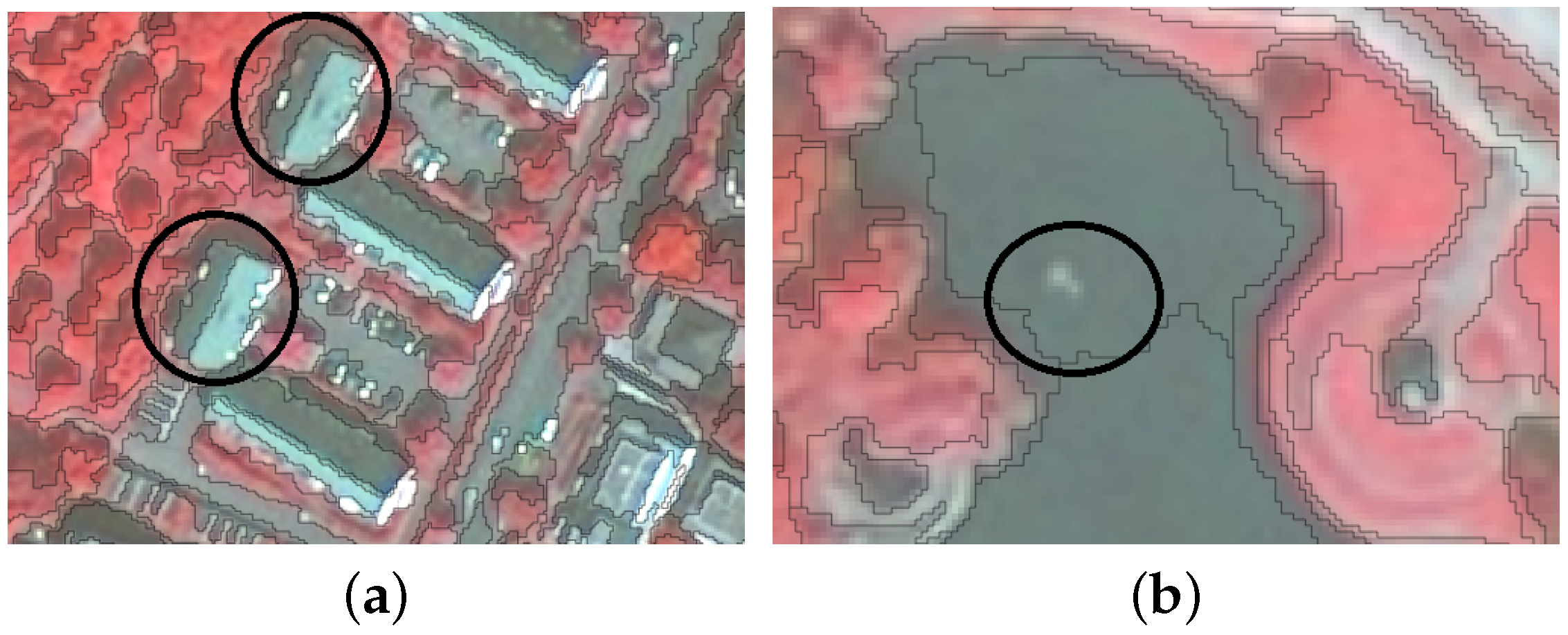
As stated in the Introduction, one of the main issues with the unsupervised analysis of VHR data is that the lack of supervision sometimes makes it difficult to map the clusters to the expert classes. One advantage of the SR-ICM algorithm is that in addition to providing a partition of the data, it returns the affinity matrix A, which gives useful information on the relationship between the clusters. The affinity matrix therefore serves a dual purpose: first it helps improve the clustering by enriching the data with neighborhood compatibility information; second, it contains low semantic level information on how the clusters relate to each other in the image. This information can either be used to help identify the expert classes or simply be translated into a description of the image once the clusters have been mapped to land cover classes.
Figure 4 shows an example of a simple affinity matrix with four clusters. In this figure, we can see how each value can be interpreted. It is easy to see how such a matrix can then be translated into a description of the image. This would lead to sentences, such as: “urban areas are surrounded by area of vegetation” or “urban areas are rarely in direct contact with water areas”, “water areas have a low compactness”, and so forth. While this may not seem like much, even this low level of description is not possible with other unsupervised algorithms.
3. Material and Methods
3.1. Presentation of the Strasbourg Dataset
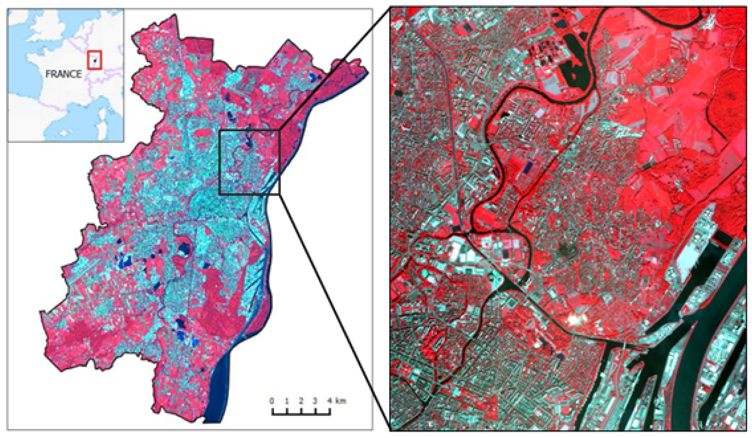
In this section, we present the data used in our experiments. The original set is an extract of a multispectral VHR pan-sharpened image with 0.5-m spatial resolution and four spectral bands (red, green, blue and near-infrared) from the Pléiades satellite Airbus, ©CNES, orthorectified and geo-referenced in Lambert93, acquired on 14 August 2012 covering the metropolitan area of Strasbourg, see Figure 5. In this article, we use only a subset of this image (9211×11,275 pixels), which is multispectral and not hyperspectral.
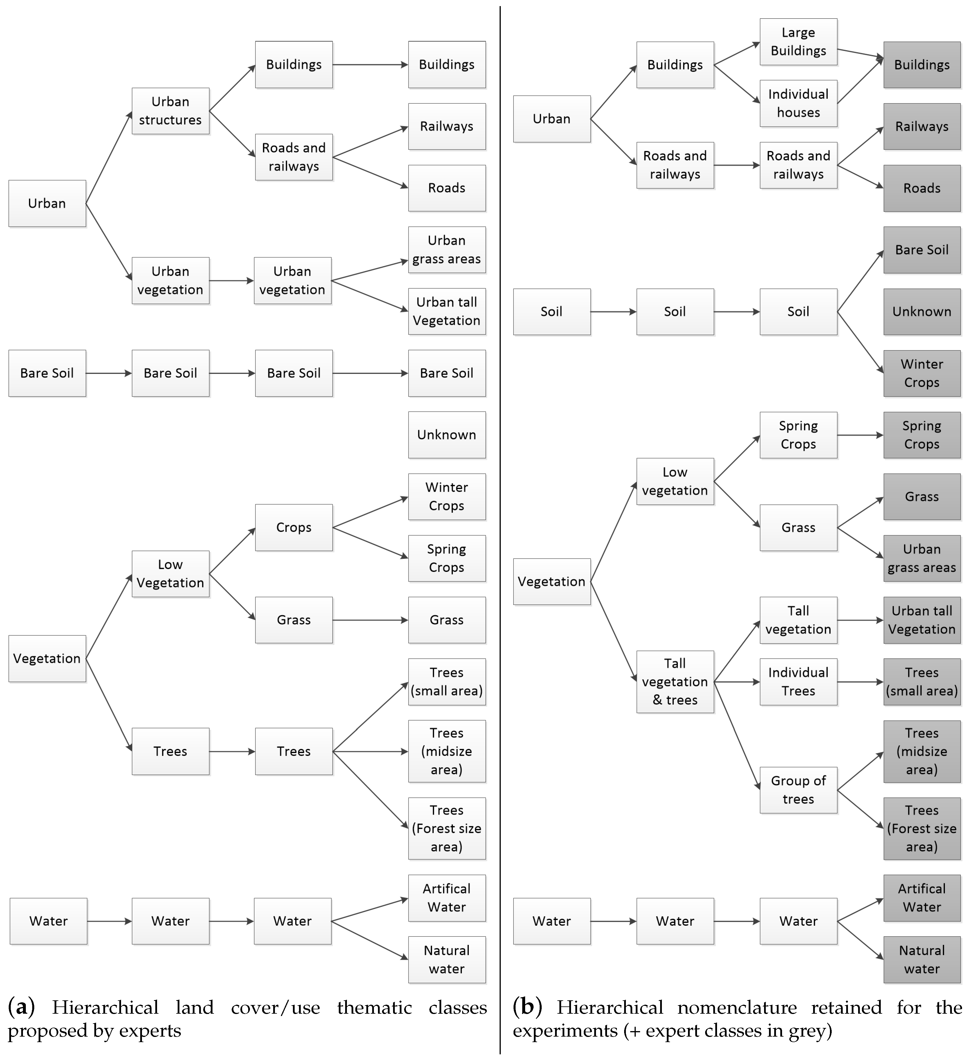
The data were later enriched with a hierarchical land cover/use database featuring 15 classes at the finest level (Level 4) from the metropolitan area of Strasbourg (Figure 6a). This database is a combination of existing vector databases (buildings, roads, railways, bare soil, crops, water) and a semi-automatic extraction of vegetation classes from several Pléiades images.
However, this hierarchical land cover/use database had to be modified because some classes such as ’grass’ and ’urban grass’ or ’bare soils’ and ’winter crops’ cannot be distinguished from the sky. Therefore, in order to propose a nomenclature adapted to an extraction from a VHR image, we have proposed the modified hierarchical typology detailed in Figure 6b. This modified database can be considered as the reference data for our research.
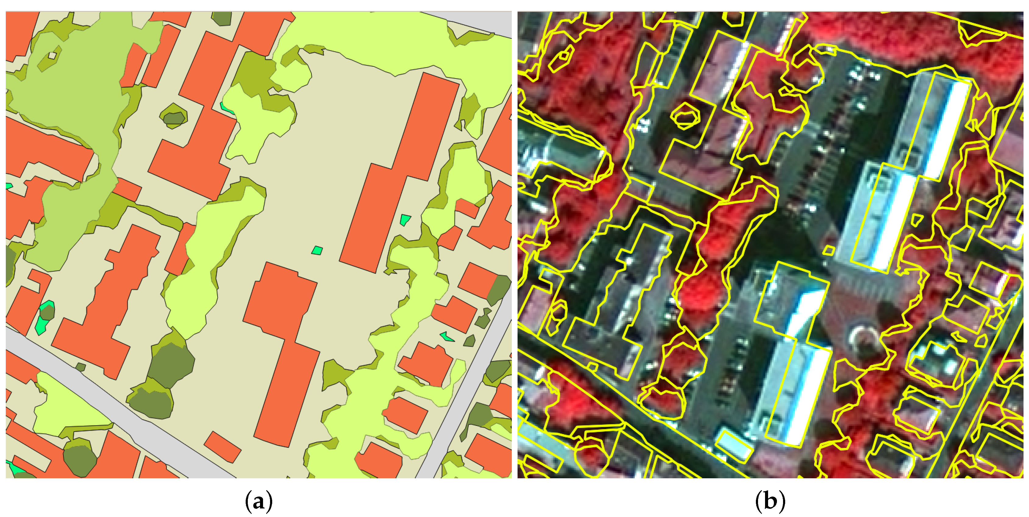
Nevertheless, some pre-processing was necessary in order to reduce the bias due to the misalignments between the land cover polygons and the Pléiades image (Figure 7): the reference data provide accurate labels, as well as very regular polygons (Figure 7a). However, when inspecting them in detail, one realizes that the polygons are not well aligned with the represented objects (Figure 7b). The misalignments are possibly due to orthorectification procedures during the pre-processing of the image or because of a date difference between the geographic information system (GIS) data and the image acquisition. Therefore, any comparison against these data would result in a difficult to quantify, yet certain bias. In order to make these data more reliable to evaluate our results, it is necessary to find a solution to improve their quality, especially in terms of segment alignment.
To cope with this issue of misaligned reference data, we propose hereafter a refining procedure that consists of superposing an over-segmentation of the image with the GIS polygons in order to propagate the GIS labels into the segments. The procedure goes as follows: for every segment in the over-segmentation, we find the set of GIS polygons intersecting . Then, it is possible to assign a single label to by taking the label of the GIS polygon with the largest intersection area with respect to . By proceeding this way, we ensure that the new reference database and the segments are actually aligned with the objects of interest, since the boundaries of the segments tend to align well with actual object boundaries. It is also possible to reinforce the quality of the produced labels by adding a threshold over the intersection area. Thus, one would only consider GIS polygons intersecting more than 50% of the area of , for example. Another possibility is to consider the labels of all intersecting polygons and to construct a fuzzy reference dataset in which each class c is weighted by the intersection area of GIS polygons labeled with class c.
In this paper, we opted to build a hard reference hybrid reference dataset using a simple majority vote.
3.2. Segmentation and Feature Computation
For our experiments, we ran the multi-resolution image segmentation (MRIS) implemented in the eCognition software ©Definens (2014) on the raw image. We chose this algorithm because it gives good performance for the retrieval of land cover/use classes [38]. MRIS is an algorithm of segmentation by “region growing”, where a scale parameter is used as the maximum heterogeneity threshold during the fusion process [11]. This heterogeneity parameter includes a spectral criterion and a shape one. Then, a level of segmentation with a scale parameter of 160 was chosen after several runs based on a statistical method developed in [39]: this method relies on the potential of the local variance to detect scale transitions in geospatial data. The tool detects the number of layers added to a project and segments them iteratively with a multi-resolution segmentation algorithm in a bottom-up approach, where the scale factor in the segmentation, namely the scale parameter, increases with a constant increment. The average local variance value of the objects in all of the layers is computed and serves as a condition for stopping the iterations: when a scale level records a local variance value that is equal to or lower than the previous value, the iteration ends, and the objects segmented in the previous level are retained.
A wide range of features available in eCognition has been computed for each segment, including spectral, textural and shape features that were exported in a CSV file. A total of 27 attributes have been calculated for 187,057 segments and are shown in Table 1, where XS1 stands for blue, XS2 green, XS3 red, and XS4 near infra-red.
3.3. Adaptation of MRF-Based Methods to a Multi-Scale Context
As we explained in the previous section, the clusters form a hierarchical structure depending on the desired level of detail. It is obvious that exploiting these hierarchical relationship between the clusters could lead to improved results and that hierarchical clustering would have the advantage of directly providing several scales of interest [2]. However, most hierarchical clustering algorithms in the literature do not handle neighborhood relationships between data and have an algorithmic complexity that is between and . Such high complexity does not scale for large datasets typically used in VHR image analysis.
To solve this problem, in our experimental section, we propose to use a modified version of the SR-ICM algorithm presented in Section 2.2. This modified version allows the user to search for different number of clusters (different scales of interest) and then runs several SR-ICM in parallel with a modified optimization function that encourages each algorithm to build hierarchical clusters depending on the other algorithms’ partitions. To this end, let us consider J scales of interest, and let us define the confusion matrix between any scales i with cluster and j with clusters so that:
The confusion matrix from Equation (4) defines how each cluster of the SR-ICM algorithm at scale i maps into the clusters of the SR-ICM algorithm at scale j. This matrix is in fact very similar to the affinity matrix from the SR-ICM model and plays the same role as a multi-scale level instead of a geographic one. From there, favoring the construction of hierarchical clusters is done by minimizing the following entropy function:
To optimize Equation (5) while ensuring that the solutions remain coherent, we modify Algorithm 1 as follows:
As one can see, Algorithm 2 is a simple parallelization of the SR-ICM algorithm presented in Algorithm 1, with a slightly modified likelihood function to which an extra prior has been added to account for the decisions made at the other scales of interest. The stopping criterion is also slightly modified, and the new criterion is that the parallel solutions found by the algorithms must be as compatible as possible. The main difference is that unlike in the original SR-ICM algorithms, the parameter is not fixed in our proposed method. As we will show bellow, this does not affect the convergence properties and has the advantages of keeping up to date clusters when using the hierarchical dependencies.
| Algorithm 2: Parallel SR-ICM for hierarchical clusters. |
 |
This algorithm has a complexity of for a dataset of size N and J different scales of interest. The convergence of the process is ensured because the algorithm optimizes the global log-likelihood function of the whole system, whose form is shown in Equation (8). In this equation, is a local log-likelihood for an algorithm at scale i, and denotes the joint entropy between the solutions at scales i and j.
Equation (8) can be transformed into Equation (9) by summing over all local likelihoods and entropies to get a global likelihood over all local models and an entropy over the whole system. Please note that is equivalent to the entropy in Equation (5).
Since we optimize Equation (9) using a maximization-maximization process over all algorithms, this is equivalent to the variational EM algorithm proposed by Neal et al. [40] and has the same convergence properties: we know that the system will converge in a finite time toward an optimum. However, we have no warranty that it will be the global optimum.
4. Experimental Results
In this section, we present the results of the clustering done from the CSV files containing the segments information, as well as the subsequent mapping to the expert classes. The experiments were therefore done on the 187,057 segments acquired from the previous steps. Each segment is described by its id, 27 geometric and radiometric attributes and its neighborhood dependencies.
Using the hierarchy established in Figure 6b, we ran three SR-ICM algorithms in parallel using Algorithm 2 searching for 4, 6 and 10 clusters. The results are shown in the next subsection.
4.1. Numerical Results
We first propose an experimental setting in which we compare our proposed method with three others from the literature: the EM algorithm using a diagonal variance-covariance matrix [37], the ICM algorithm using the Gaussian mixture model and a regular prior [35], the regular non multiscale SR-ICM algorithm [3] and the SOM algorithm for VHR images [4].
We ran a dozen simulations with each algorithm for the three scales of interest with 4, 6 and 10 clusters. In Table 2, we show the results of these simulation with the average values for four different indexes:
- The Davies–Bouldin index [41]: It is a clustering index assessing that the clusters are compact and well separated. Its value is better when it is lower and tends to be biased towards a lower number of clusters.
- The silhouette index [42]: It is another clustering index assessing that each datum is closer to its clusters centroid than from the other clusters’. It takes its values between −1 and one and is better when closer to one.
- The Rand index [43]: It is an external index assessing the degree of similitude between two vectors. In the case of this experiment, we compared our solution vectors with our GIS hybrid reference data. It takes its values between zero and one, with one being a 100% match.
- An entropy measure assessing the entropy between each algorithm solutions and the GIS hybrid reference data using the confusion matrix as shown in Equation (10). It takes its values between zero and one, with zero being a 100% match and achievable only if the solution and the reference data have the same number of classes/clusters. This measure is therefore better when close to zero and is biased toward a greater number of clusters.
Note that in Equation (10), we use the value of 15, because there are 15 classes in the expert reference data.
From Table 2, we can draw several conclusions: First, if we look at the unsupervised indexes (Davies–Bouldin and silhouette), we can see that the expectation-maximization algorithm mostly outperforms all algorithms. This result was to be expected in the sense that both indexes assess the quality of clusters and that the EM algorithm is the only “pure” clustering method that we used here. All three variations of the ICM use spatial dependencies to bend the original clusters toward more realistic classes, hence the degradation that we observe in the unsupervised indexes. It is therefore logical that the EM algorithm has the best results for unsupervised indexes. It is followed by the GMM-ICM and SR-ICM with their modified priors. Then comes the SOM algorithm. Finally, our proposed multi-scale SR-ICM is lagging behind because it has two priors that further bend the partitions away from the usual spherical and well-separated clusters.
This leads us to the interpretation of the supervised indexes (Rand index and entropy). Given the final goal of our application, which is the automatic classification (and not the clustering) of objects in very high resolution images, it is these two indexes that matter most for real applications. As one can see, the results are reversed: our proposed ms-SR-ICM algorithm slightly outperforms both other ICM algorithms; the SOM algorithm still has average performances; and the EM algorithm scores last.
In terms of performances, our proposed parallelized multi-scale version of the semantic-rich ICM algorithm achieves the lowest entropies on the three scales of interest and up to an 80% match with the reference data, which is approximately 2% ahead of the second best algorithm. We also note that on the four clusters’ scale, there is no difference between the results of the three ICM algorithms. There are two possible explanations for these results: First, with only four clusters compared with the 15 reference classes, the Rand Index may not be able to discriminate between the algorithms. Second, multi-scale approaches are known to favor scales with more clusters: it is easier to check that clusters have been properly divided from a scale with less clusters because there is less information dispersion than checking that they have been properly merged from a scale with more clusters. Therefore, our proposed method is mostly beneficial for the six clusters and 10 clusters scales.
Beyond the efficiency of our proposed method, this experiment highlights that there is a strong disconnection between clustering indexes that are used by most unsupervised methods and the supervised indexes that are used in real applications. This difficulty that we have been discussing since the Introduction is a real challenge for the conception of future automated detection systems.
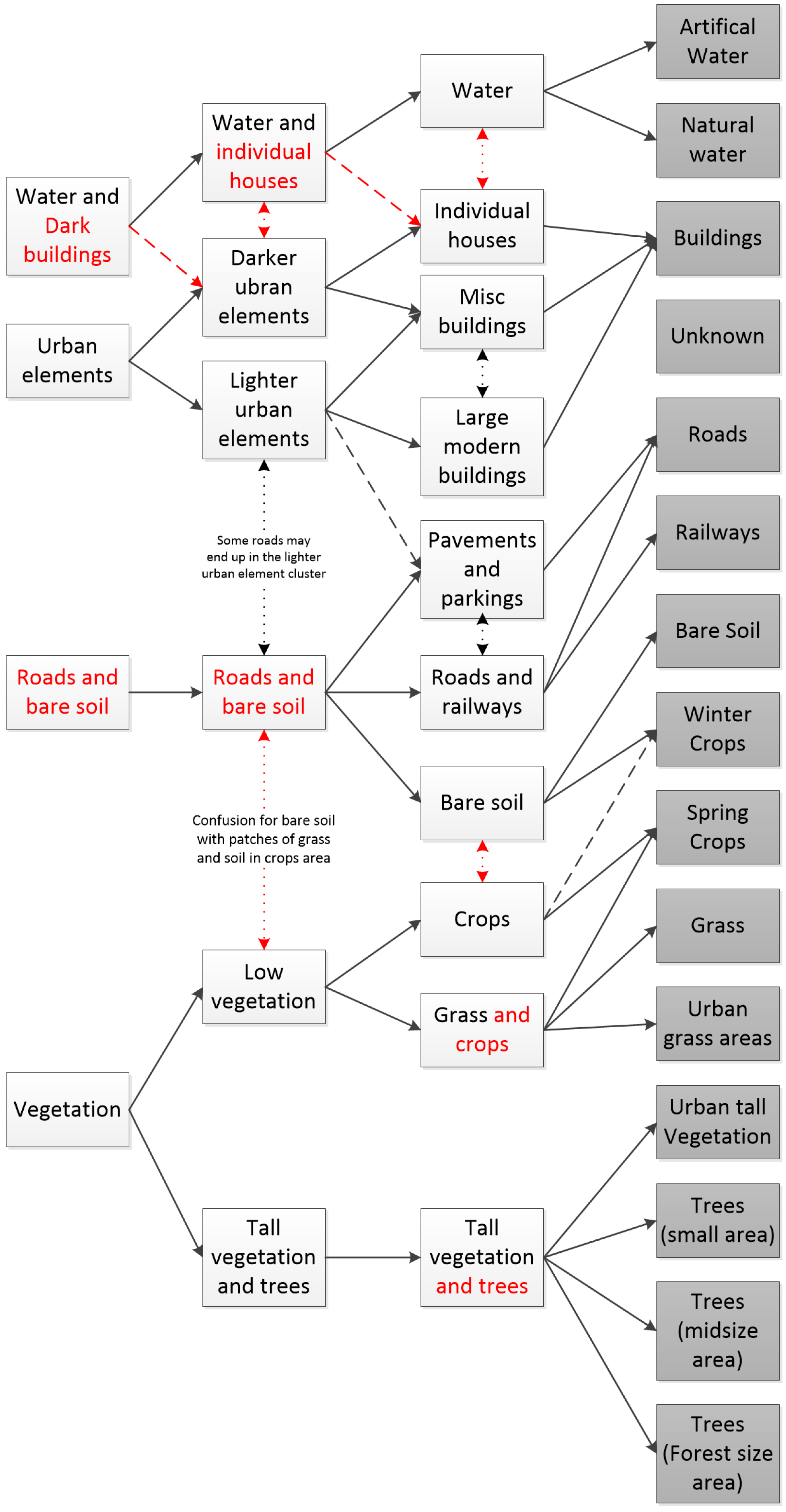
In Figure 8, we show the typical hierarchical clusters found by our proposed method.
As one can see, the two main differences with Figure 6 come from the inclusion of road elements grouped with bare soil areas at scales of four and six clusters and from the difficulty to properly separate water from a dark building and then individual houses at the same scales. Our explanation for the difference in the hierarchy is the following: Unlike in pixel-based clustering where only color attributes are considered, leading to easily separating water from the other classes, our OBIA approach uses a larger number of non-color based attributes, which delay this separation. While color-based attributes are still the most influential, since we use the Euclidean distance, in which all features have the same weight, their discrimination power is significantly reduced. Consequently, our four first clusters regroup elements that have close enough colors and shapes, thus regrouping the water (dark blue) and some dark urban elements (dark grey and black) in the first cluster, brighter (light grey or white) urban elements in another, roads and bare soil (brown and grey) in a third one and vegetation (green) in the final cluster. Then, at the six clusters’ scale, the shape of the segments seems to become significant enough to separate most large darker buildings from the water cluster.
On the other hand, small individual houses with blue tiled roofs or shadow areas have segments whose shape is very similar to water areas. Furthermore, all three tend to be surrounded by a similar vegetation environment, thus making the differentiation difficult even using the neighborhood semantic matrix. Therefore, a decent separation of the water from the other elements is only achieved at the 10 clusters’ scale. While this may be problematic in the sense that the supervised algorithm usually learns first to detect water, in the case of unsupervised learning, this was to be expected, since there is no supervision at all. Other unsupervised algorithms applied to OBIA suffer from the same issue as satellite images [3,4], but our method still handles this problem when there are enough clusters.
Other minor flaws when comparing the clustering to what could have been expected from a supervised algorithm include: The regrouping of roads and bare soil in the same cluster; the different types of tree areas generally grouped in a single cluster. However, this matched with the reference data and therefore is not really a problem; the confusions that occurs between some bare soil and vegetation areas due to the fact that there may be patches of grass or crops in bare soil areas and patches of bare soil in crops and low vegetation areas. This problem is in our opinion impossible to solve without changing the segmentation.
Our proposed method also created some unexpected clusters, such as one containing large modern buildings (mostly industrial buildings) and another one differentiating roads from parking and pavements (based on the cluster’s shape and semantic surrounding). In fact, our method gives three types of buildings where the expert found only one and where we expected to find only two. Furthermore, except for the minor confusions between crops and low vegetation, the hierarchical tree found by our method globally matches the one given in Figure 6.
4.2. Visual Results
In this section, we show some visual extracts of the results obtained by our method and the algorithms used in the previous section. As such, the explanations that follow are purely based on our interpretation of these visual results. To get the exact accuracy of the clusters displayed in Figure 9 and Figure 10, you can refer to the “Rand index” column of Table 2.
In Figure 9, we show the visual result of our method looking for six clusters in the center area of the city of Strasbourg. Our results are compared with these of two others algorithms from the literature. We tried to use similar color codes for all figures despite the variety of classes and clusters: blue is used for water, different scales of green and yellow for vegetation areas, grey for roads, pink and violet for buildings.
If we first look at Figure 9b with the raw polygons and Figure 9c with the hybrid reference data, we can see that the original GIS reference data of this area in Figure 9b have much less and more linear objects than the segmentation Figure 9c. For this reason, the hybrid ground-truth shown in Figure 9c features large homogeneous areas of the same class that clearly should be separated when we look at the original image in Figure 9a. This is a visual confirmation that our ground-truth used for Table 2 is not perfect and further explains why this hybrid ground-truth cannot be used for supervised learning.
Moving to Figure 9d–f, we can see a comparison between one of our SR-ICM results at the scale with six clusters and the visualization of a result from the SOM algorithm [4] and EM algorithm using the Gaussian mixture model for the same area. First, we can see in Figure 9d that our algorithm correctly detects the river, whereas the SOM algorithm (Figure 9e) only partially does so, and the EM algorithm Figure 9f fails to do so. The same can be said for the stadium on the top right of the image. We can see that all three algorithms mostly correctly identify vegetation areas, with the EM algorithm making slightly more mistakes. Finally, all three algorithms make several confusions between individual houses and water areas due to the roofs’ color as we had already mentioned when commenting on Figure 8. This proves that this issue is not isolated to our method.
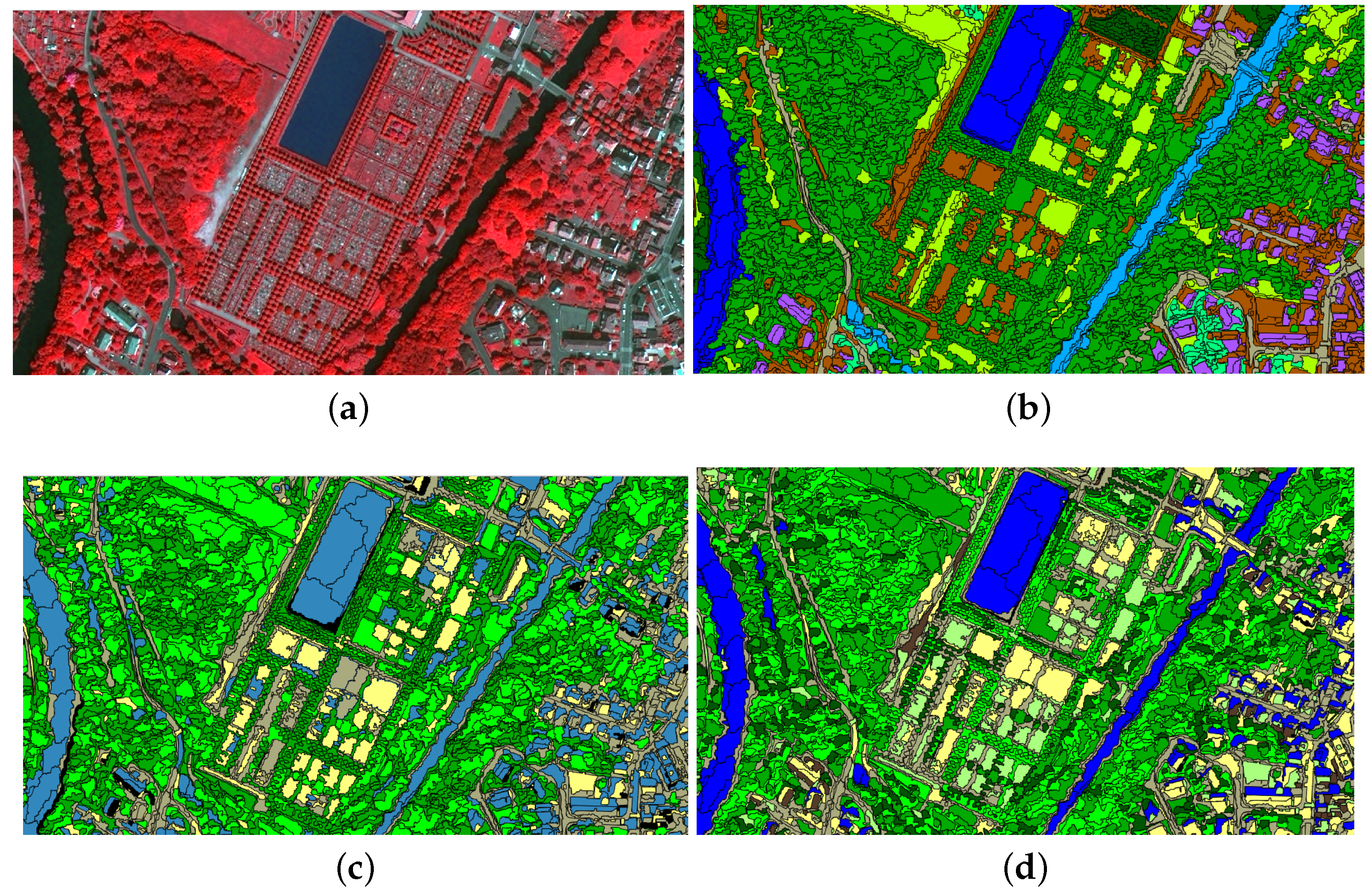
In Figure 10, we show the result of our algorithms at scales of six and 10 clusters when applied to a non-urban area of our satellite image. As we can see, while the confusion between water and individual houses is less frequent at the 10 clusters’ scales, it remains present for several segments. Nevertheless, several areas are correctly classified: roads, rivers and several types of vegetation areas.
4.3. Discussion
We now would like to conclude this experimental section. For the clustering step, our proposed method uses a multi-scale analysis that is both adapted to this type of images, but also helps achieve better results. We have compared our method with three other methods available from the literature, and while we have seen that our method still has flaws (also found in other unsupervised methods), our algorithm achieves better results in terms of supervised indexes, unsupervised indexes and also visual results.
It is true that the results in terms of supervised and unsupervised indexes are not overwhelming when compared to those of other methods, but the projection of our results on the original images makes it clear that our method gives the best results. Furthermore, our algorithm has the advantage of keeping both the semantic analysis aspect of the original SR-ICM algorithm and to add the description of the cluster hierarchy at different scales. This latter addition is extremely valuable to interpret the strengths and weaknesses of our method and helps to adjust the algorithms’ parameters to achieve the best possible results.
Possible future works to improve the results of our method, both during the segmentation step and the clustering step, could include a pre-selection of the attributes of interest based on saliency criteria at the considered scale. To this end, several inspiring works exist in hyperspectral image analysis [44,45] to select the optimal bands. These works could be adapted to weight attributes instead of bands and may lead to improved results.
5. Conclusions
In this article, we have been concerned with the challenges and issues that lie with the unsupervised analysis of very high resolution satellite images. After an overview of the different steps to achieve this goal and a short summary of the methods available in the literature with their strengths and weaknesses, we have proposed our own contribution in the form of a multi-scale version of the semantic-rich ICM algorithm that covers the need for multi-scale algorithms to analyze very high resolution images.
In order to demonstrate the efficiency of our method, we have detailed the step by step processing of a satellite image of the French city of Strasbourg, using methods available from the literature for the cleaning and segmentation steps and then comparing our proposed method to others during the unsupervised analysis of the images segments with the goal of finding the final classes of interests at several scales. During these steps, we have highlighted the difficulties encountered by all methods including ours.
In addition to its low computational complexity and the ease to choose the scales of interest to which to apply a clustering process, our method has shown competitive performances when compared to other state of the art algorithms. Furthermore, our proposed algorithm retains low level semantic information that can be easily used to map the clusters to the expert classes of interest.
In our future work, we look forward to proposing similar multi-scale implementations during the segmentation step of a satellite image with the goal of producing better segments, thus reducing the accumulation of errors during the different steps of the image processing. It would also be interesting to use feature selection criteria in order to better detect objects of interest at the different scales, but also to avoid using redundant attributes.
Acknowledgments
This work has been supported by the ANR project COCLICO , ANR-12-MONU-0001. The authors would like to thank the Pléiades Users Thematic Commissioning, Program ORFEO (Optical and Radar Federated Earth Observation) Accompaniment Program (CNES), for Pléiades images availability. Thanks to the metropolitan area of Strasbourg for the land cover/use database used as reference data for our experiments.
Author Contributions
Anne Puissant is one of the main contributors in creating most of the source material for the ANR project COCLICO and this paper. She has also worked in collaboration with Simon Rougier (LIVE laboratory ) on the segmentation step that produced the CSV file with feature data used in this paper. Andrés Troya-Galvis has participated in the creation of the CSV files describing the segments used for the unsupervised learning part of this article, as well as the creation of the hybrid reference data. Jérémie Sublime designed the unsupervised algorithms introduced in this article (several of them are from his PhD thesis) and ran all clustering experiments proposed in this work. The paper was co-written by all three authors.
Conflicts of Interest
The authors declare no conflict of interest. The ANR funding sponsor had no role in designing the study or the experiments, nor in the decision to write and publish this paper.
Abbreviations
The following abbreviations are used in this manuscript:
| ANR | “Agence Nationale de la Recherche” (French National Agency for Research) |
| EM | Expectation maximization |
| GIS | Geographic information systems |
| ICM | Iterated conditional modes |
| MRF | Markov random fields |
| MRIS | Multi-resolution image segmentation |
| OBIA | Object-based image analysis |
| VHR | Very high resolution |
References
- Blaschke, T. Object based image analysis for remote sensing. ISPRS J. Photogramm. Remote Sens. 2010, 65, 2–16. [Google Scholar] [CrossRef]
- d’Oleire-Oltmanns, S.; Eisank, C.; Dragut, L.; Blaschke, T. An Object-Based Workflow to Extract Landforms at Multiple Scales from Two Distinct Data Types. IEEE Geosci. Remote Sens. Lett. 2013, 10, 947–951. [Google Scholar] [CrossRef]
- Sublime, J.; Troya-Galvis, A.; Bennani, Y.; Gancarski, P.; Cornuéjols, A. Semantic Rich ICM Algorithm for VHR Satellite Image Segmentation. In Proceedings of the IAPR International Conference on Machine Vision Applications (MVA 2015), Tokyo, Japan, 18–22 May 2015. [Google Scholar]
- Grozavu, N.; Rogovschi, N.; Cabanes, G.; Troya-Galvis, A.; Gançarski, P. VHR satellite image segmentation based on topological unsupervised learning. In Proceedings of the 14th IAPR International Conference on Machine Vision Applications, Tokyo, Japan, 18–22 May 2015; pp. 543–546. [Google Scholar]
- Pal, N.R.; Pal, S.K. A review on image segmentation techniques. Pattern Recognit. 1993, 26, 1277–1294. [Google Scholar] [CrossRef]
- Gonzalez, R.C.; Woods, R.E. Digital Image Processing, 3rd ed.; Prentice-Hall, Inc.: Upper Saddle River, NJ, USA, 2006. [Google Scholar]
- Cheng, H.; Jiang, X.; Sun, Y.; Wang, J. Color image segmentation: Advances and prospects. Pattern Recognit. 2001, 34, 2259–2281. [Google Scholar] [CrossRef]
- Comaniciu, D.; Meer, P. Mean shift: A robust approach toward feature space analysis. IEEE Trans. Pattern Anal. Mach. Intell. 2002, 24, 603–619. [Google Scholar] [CrossRef]
- Michel, J.; Youssefi, D.; Grizonnet, M. Stable mean-shift algorithm and its application to the segmentation of arbitrarily large remote sensing images. IEEE Trans. Geosci. Remote Sens. 2015, 53, 952–964. [Google Scholar] [CrossRef]
- Fukunaga, K.; Hostetler, L. The estimation of the gradient of a density function, with applications in pattern recognition. IEEE Trans. Inf. Theory 1975, 21, 32–40. [Google Scholar] [CrossRef]
- Baatz, M.; Schäpe, A. Multiresolution Segmentation: An optimization approach for high quality multi-scale image segmentation. In Angewandte Geographische Informationsverarbeitung XII. Beiträge zum AGIT-Symposium Salzburg 2000; Strobl, J., Ed.; Herbert Wichmann Verlag: Karlsruhe, Germany, 2000; pp. 12–23. [Google Scholar]
- Wang, Z.; Jensen, J.R.; Im, J. An automatic region-based image segmentation algorithm for remote sensing applications. Environ. Model. Softw. 2010, 25, 1149–1165. [Google Scholar] [CrossRef]
- Derivaux, S.; Forestier, G.; Wemmert, C.; Lefèvre, S. Supervised image segmentation using watershed transform, fuzzy classification and evolutionary computation. Pattern Recognit. Lett. 2010, 31, 2364–2374. [Google Scholar] [CrossRef]
- Li, D.; Zhang, G.; Wu, Z.; Yi, L. An edge embedded marker-based watershed algorithm for high spatial resolution remote sensing image segmentation. IEEE Trans. Image Process. 2010, 19, 2781–2787. [Google Scholar] [PubMed]
- Peng, B.; Zhang, L.; Zhang, D. A survey of graph theoretical approaches to image segmentation. Pattern Recognit. 2013, 46, 1020–1038. [Google Scholar] [CrossRef]
- Paglieroni, D.W. Design considerations for image segmentation quality assessment measures. Pattern Recognit. 2004, 37, 1607–1617. [Google Scholar] [CrossRef]
- Corcoran, P.; Winstanley, A.; Mooney, P. Segmentation performance evaluation for object-based remotely sensed image analysis. Int. J. Remote Sens. 2010, 31, 617–645. [Google Scholar] [CrossRef]
- Srubar, S. Quality Measurement of Image Segmentation Evaluation Methods. In Proceedings of the 2012 Eighth International Conference on Signal Image Technology and Internet Based Systems (SITIS), Naples, Italy, 25–29 November 2012; pp. 254–258. [Google Scholar]
- Zhang, X.; Xiao, P.; Feng, X. An Unsupervised Evaluation Method for Remotely Sensed Imagery Segmentation. IEEE Geosci. Remote Lett. 2012, 9, 156–160. [Google Scholar] [CrossRef]
- Johnson, B.; Xie, Z. Unsupervised image segmentation evaluation and refinement using a multi-scale approach. ISPRS J. Photogramm. 2011, 66, 473–483. [Google Scholar] [CrossRef]
- Troya-Galvis, A.; Gançarski, P.; Passat, N.; Berti-Équille, L. Unsupervised quantification of under and over segmentation for object based remote sensing image analysis. IEEE J. Sel. Top. Appl. Earth Obs. Remote Sens. 2015, 8, 1936–1945. [Google Scholar] [CrossRef]
- Liu, N.; Li, J.; Li, N. A Graph-segment-based Unsupervised Classification for Multispectral Remote Sensing Images. WSEAS Trans. Inf. Sci. Appl. 2008, 5, 929–938. [Google Scholar]
- Asmus, V.V.; Buchnev, A.A.; Pyatkin, V.P. Cluster analysis of earth remote sensing data. Optoelectron. Instrum. Data Process. 2010, 46, 149–155. [Google Scholar] [CrossRef]
- He, H.; Liang, T.; Hu, D.; Yu, X. Remote sensing clustering analysis based on object-based interval modeling. Comput. Geosci. 2016, 94, 131–139. [Google Scholar] [CrossRef]
- Li, H.; Zhang, S.; Ding, X.; Zhang, C.; Dale, P. Performance Evaluation of Cluster Validity Indices (CVIs) on Multi/Hyperspectral Remote Sensing Datasets. Remote Sens. 2016, 8, 295. [Google Scholar] [CrossRef]
- Chahdi, H.; Grozavu, N.; Mougenot, I.; Berti-Equille, L.; Bennani, Y. On the Use of Ontology as a priori Knowledge into Constrained Clustering. In Proceedings of the IEEE International Conference on Data Science and Advanced Analytics (DSAA), Montreal, QC, Canada, 17–19 October 2016. [Google Scholar]
- Chahdi, H.; Grozavu, N.; Mougenot, I.; Bennani, Y.; Berti-Equille, L. Towards Ontology Reasoning for Topological Cluster Labeling. ICONIP (3). In Lecture Notes in Computer Science; Hirose, A., Ozawa, S., Doya, K., Ikeda, K., Lee, M., Liu, D., Eds.; Springer: Cham, Switzerland, 2016; Volume 9949, pp. 156–164. [Google Scholar]
- Roth, S.; Black, M.J. Fields of experts. In Markov Random Fields for Vision and Image Processing; Blake, A., Kohli, P., Rother, C., Eds.; MIT Press: Cambridge, MA, USA, 2011; pp. 297–310. [Google Scholar]
- Ardila, J.; Tolpekin, V.; Bijker, W. Markov random field based super-resolution mapping for identification of urban trees in VHR images. In Proceedings of the IEEE International Geoscience & Remote Sensing Symposium, Honolulu, HI, USA, 25–30 July 2010; pp. 1402–1405. [Google Scholar]
- Sublime, J.; Cornuéjols, A.; Bennani, Y. A New Energy Model for the Hidden Markov Random Fields; Lecture Notes in Computer Science; Springer: Cham, Switzerland, 2014; Volume 8835, pp. 60–67. [Google Scholar]
- Boykov, Y.; Veksler, O.; Zabih, R. Fast Approximate Energy Minimization via Graph Cuts. IEEE Trans. Pattern Anal. Mach. Intell. 2001, 23, 1222–1239. [Google Scholar] [CrossRef]
- Leordeanu, M.; Hebert, M.; Sukthankar, R. An Integer Projected Fixed Point Method for Graph Matching and MAP Inference. In Proceedings of the Advances in Neural Information Processing Systems 22: 23rd Annual Conference on Neural Information Processing Systems, Vancouver, BC, Canada, 7–10 December 2009; Bengio, Y., Schuurmans, D., Lafferty, J.D., Williams, C.K.I., Culotta, A., Eds.; Curran Associates, Inc.: Red Hook, NY, USA, 2009; pp. 1114–1122. [Google Scholar]
- Liu, Z.Y.; Qiao, H.; Su, J.H. Neural Information Processing: 21st International Conference, ICONIP 2014, Kuching, Malaysia, November 3–6, 2014. Proceedings, Part II; Springer: Cham, Switzerland, 2014; pp. 404–412. [Google Scholar]
- Besag, J. On the statistical analysis of dirty pictures. J. R. Stat. Soc. Ser. B 1986, 48, 259–302. [Google Scholar] [CrossRef]
- Zhang, Y.; Brady, M.; Smith, S.M. Segmentation of Brain MR Images through a Hidden Markov Random Field Model and the Expectation Maximization Algorithm. IEEE Trans. Med. Imaging 2001, 20, 45–57. [Google Scholar] [CrossRef] [PubMed]
- Xu, K.; Yang, W.; Liu, G.; Sun, H. Unsupervised Satellite Image Classification Using Markov Field Topic Model. IEEE Geosci. Remote Sens. Lett. 2013, 10, 130–134. [Google Scholar] [CrossRef]
- Dempster, A.P.; Laird, N.M.; Rubin, D.B. Maximum likelihood from incomplete data via the EM algorithm. J. R. Stat. Soc. Ser. B 1977, 39, 1–38. [Google Scholar]
- Puissant, A.; Rougier, S.; Stumpf, A. Object-oriented mapping of urban trees using Random Forest classifiers. Int. J. Appl. Earth Obs. Geoinf. 2014, 26, 235–245. [Google Scholar] [CrossRef]
- Dragut, L.; Csillik, O.; Eisank, C.; Tiede, D. Automated parameterisation for multi-scale image segmentation on multiple layers. ISPRS J. Photogramm. Remote Sens. 2014, 88, 119–127. [Google Scholar] [CrossRef] [PubMed]
- Neal, R.M.; Hinton, G.E. A view of the EM algorithm that justifies incremental, sparse, and other variants. In Learning in Graphical Models; Springer: Cham, The Netherlands, 1998; pp. 355–368. [Google Scholar]
- Davies, D.L.; Bouldin, D.W. A Cluster Separation Measure. IEEE Trans. Pattern Anal. Mach. Intell. 1979, 1, 224–227. [Google Scholar] [CrossRef] [PubMed]
- Rousseeuw, P.J.; Leroy, A.M. Robust Regression and Outlier Detection; John Wiley & Sons, Inc.: New York, NY, USA, 1987. [Google Scholar]
- Rand, W. Objective criteria for the evaluation of clustering methods. J. Am. Stat. Assoc. 1971, 66, 846–850. [Google Scholar] [CrossRef]
- Yuan, Y.; Lin, J.; Wang, Q. Dual-Clustering-Based Hyperspectral Band Selection by Contextual Analysis. IEEE Trans. Geosci. Remote Sens. 2016, 54, 1431–1445. [Google Scholar] [CrossRef]
- Wang, Q.; Lin, J.; Yuan, Y. Salient Band Selection for Hyperspectral Image Classification via Manifold Ranking. IEEE Trans. Neural Netw. Learn. Syst. 2016, 27, 1279–1289. [Google Scholar] [CrossRef] [PubMed]
Figure 1.
Step by step approach to image processing.

Figure 2.
Examples of over-segmentation and under-segmentation. (a) Example of an over-segmentation on two houses that could be fixed during the clustering step: the algorithm may still detect that these two segments are part of the same cluster; (b) example of an under-segmentation where the white object in the middle of the lake was not detected during the segmentation step and will never be since it is now merged with a lake segment.

Figure 3.
Illustration of the MRF clustering problem with very few features: in this example, we try to guess the cluster of the central segment based on five features and the clusters of its neighbor segments (identified using the colors).
Figure 3.
Illustration of the MRF clustering problem with very few features: in this example, we try to guess the cluster of the central segment based on five features and the clusters of its neighbor segments (identified using the colors).

Figure 4.
Example of an affinity matrix: Diagonal values indicate whether or not the clusters are forming compact areas (high value) or are scattered elements in the image (low value). Non-diagonal elements indicate which clusters are often neighbors on the image (high value) or incompatible neighbors (low value).

Figure 5.
(Left) the metropolitan area of Strasbourg (Spotimage ©CNES, 2012); (right) extract of the Pan-sharpened Pléiades image (Airbus ©CNES, 2012).
Figure 5.
(Left) the metropolitan area of Strasbourg (Spotimage ©CNES, 2012); (right) extract of the Pan-sharpened Pléiades image (Airbus ©CNES, 2012).

Figure 6.
Expert classes (a) and hierarchical classes retained for the experiments (b).

Figure 7.
Example of reference data from geographic information systems (GIS). (a) GIS labeled data; (b) contours of the GIS polygons.
Figure 7.
Example of reference data from geographic information systems (GIS). (a) GIS labeled data; (b) contours of the GIS polygons.

Figure 8.
Expert classes in grey (right) and hierarchical clusters extracted from the confusion matrices found by our proposed method (left): The plain arrows highlight strong links, dashed arrows mild links and dotted arrows weak links. The arrows and characters in red highlight potentially armful errors in the clusters or their hierarchy when compared with the expected classes.

Figure 9.
Original image (extract), reference data images and results using different algorithms looking for six clusters. (a) Original image, Pléiades ©Airbus, CNES 2012; (b) reference data ©EMS 2012: raw polygons; (c) hybrid reference data; (d) multi-scale SR-ICM at the six clusters’ scale; (e) SOM algorithm [4] with six clusters; (f) EM algorithm with six clusters.

Figure 10.
Original image (extract), reference data and our algorithm at scales of six and 10 clusters. (a) Original image, Pléiades ©Airbus, CNES 2012; (b) hybrid reference data; (c) multi-scale SR-ICM at the six clusters’ scale; (d) multi-scale SR-ICM at the 10 clusters’ scale.
Figure 10.
Original image (extract), reference data and our algorithm at scales of six and 10 clusters. (a) Original image, Pléiades ©Airbus, CNES 2012; (b) hybrid reference data; (c) multi-scale SR-ICM at the six clusters’ scale; (d) multi-scale SR-ICM at the 10 clusters’ scale.


Table 1.
The 27 attributes computed for the 187,057 segments.
| Attribute | Type | Comments |
|---|---|---|
| Brightness | Spectral | |
| Max. difference | Spectral | |
| Mean XS1 | Spectral | Blue |
| Mean XS2 | Spectral | Green |
| Mean XS3 | Spectral | Red |
| Mean XS4 | Spectral | near-infrared |
| Standard deviation XS1 | Spectral | Blue |
| Standard deviation XS2 | Spectral | Green |
| Standard deviation XS3 | Spectral | Red |
| Standard deviation XS4 | Spectral | Near-infrared |
| Ratio XS1 | Spectral | Blue |
| Ratio XS2 | Spectral | Green |
| Ratio XS3 | Spectral | Red |
| Ratio XS4 | Spectral | Near-infrared |
| Mean Diff. to neighbors XS1 | Spectral | Blue |
| Mean Difference to neighbors XS2 | Spectral | Green |
| Mean Difference to neighbors XS3 | Spectral | Red |
| Mean Difference to neighbors XS4 | Spectral | Near-infrared |
| Area | Shape | in pixels |
| Elliptic fit | Shape | |
| Density | Shape | |
| Rectangular Fit | Shape | |
| Shape index | Shape | |
| Asymmetry | Shape | |
| Gray level co-occurrence matrix contrast (all dir.) | Textural | |
| Gray level co-occurrence matrix entropy (all dir.) | Textural | |
| Gray level co-occurrence matrix correlation (all dir.) | Textural |
Table 2.
Comparative results of our proposed “multi-scale semantic-rich iterated conditional modes (ms-SR-ICM)” approach with other methods of the literature using 2 internal indexes and 2 external indexes. SOM, self-organizing map.
Table 2.
Comparative results of our proposed “multi-scale semantic-rich iterated conditional modes (ms-SR-ICM)” approach with other methods of the literature using 2 internal indexes and 2 external indexes. SOM, self-organizing map.
| Algorithm | Davies–Bouldin Index | Silhouette Index | Rand Index | Entropy |
|---|---|---|---|---|
| EM (4 clusters) | 2.09 | 0.23 | 0.69 | 0.64 |
| EM (6 clusters) | 2.10 | 0.19 | 0.72 | 0.62 |
| EM (10 clusters) | 2.59 | 0.11 | 0.70 | 0.61 |
| GMM-ICM (4 clusters) | 3.65 | 0.14 | 0.72 | 0.59 |
| GMM-ICM (6 clusters) | 2.52 | 0.16 | 0.73 | 0.58 |
| GMM-ICM (10 clusters) | 3.92 | 0.07 | 0.75 | 0.58 |
| SR-ICM (4 clusters) | 4.16 | 0.15 | 0.72 | 0.58 |
| SR-ICM (6 clusters) | 2.49 | 0.19 | 0.75 | 0.58 |
| SR-ICM (10 clusters) | 3.50 | 0.10 | 0.78 | 0.57 |
| ms-SR-ICM (4 clusters) | 4.27 | 0.14 | 0.72 | 0.57 |
| ms-SR-ICM (6 clusters) | 2.47 | 0.20 | 0.77 | 0.57 |
| ms-SR-ICM (10 clusters) | 3.33 | 0.10 | 0.80 | 0.55 |
| SOM (6 clusters) | 2.23 | 0.17 | 0.75 | 0.60 |
| SOM (10 clusters) | 4.04 | 0.05 | 0.75 | 0.63 |
© 2017 by the authors. Licensee MDPI, Basel, Switzerland. This article is an open access article distributed under the terms and conditions of the Creative Commons Attribution (CC BY) license (http://creativecommons.org/licenses/by/4.0/).
Share and Cite
MDPI and ACS Style
Sublime, J.; Troya-Galvis, A.; Puissant, A. Multi-Scale Analysis of Very High Resolution Satellite Images Using Unsupervised Techniques. Remote Sens. 2017, 9, 495. https://0-doi-org.brum.beds.ac.uk/10.3390/rs9050495
AMA Style
Sublime J, Troya-Galvis A, Puissant A. Multi-Scale Analysis of Very High Resolution Satellite Images Using Unsupervised Techniques. Remote Sensing. 2017; 9(5):495. https://0-doi-org.brum.beds.ac.uk/10.3390/rs9050495
Chicago/Turabian StyleSublime, Jérémie, Andrés Troya-Galvis, and Anne Puissant. 2017. "Multi-Scale Analysis of Very High Resolution Satellite Images Using Unsupervised Techniques" Remote Sensing 9, no. 5: 495. https://0-doi-org.brum.beds.ac.uk/10.3390/rs9050495
Note that from the first issue of 2016, this journal uses article numbers instead of page numbers. See further details here.