
Learning Dual Multi-Scale Manifold Ranking for Semantic Segmentation of High-Resolution Images

1
School of Remote Sensing and Information Engineering, 129 Luoyu Road, Wuhan University, Wuhan 430079, China
2
Collaborative Innovation Center of Geospatial Technology, Wuhan University, Wuhan 430079, China
3
School of Resource and Environmental Sciences, 129 Luoyu Road, Wuhan University, Wuhan 430079, China
*
Author to whom correspondence should be addressed.
Remote Sens. 2017, 9(5), 500; https://0-doi-org.brum.beds.ac.uk/10.3390/rs9050500
Submission received: 9 March 2017
/
Revised: 12 May 2017
/
Accepted: 12 May 2017
/
Published: 19 May 2017
(This article belongs to the Special Issue Learning to Understand Remote Sensing Images)
Abstract
:Semantic image segmentation has recently witnessed considerable progress by training deep convolutional neural networks (CNNs). The core issue of this technique is the limited capacity of CNNs to depict visual objects. Existing approaches tend to utilize approximate inference in a discrete domain or additional aides and do not have a global optimum guarantee. We propose the use of the multi-label manifold ranking (MR) method in solving the linear objective energy function in a continuous domain to delineate visual objects and solve these problems. We present a novel embedded single stream optimization method based on the MR model to avoid approximations without sacrificing expressive power. In addition, we propose a novel network, which we refer to as dual multi-scale manifold ranking (DMSMR) network, that combines the dilated, multi-scale strategies with the single stream MR optimization method in the deep learning architecture to further improve the performance. Experiments on high resolution images, including close-range and remote sensing datasets, demonstrate that the proposed approach can achieve competitive accuracy without additional aides in an end-to-end manner.
1. Introduction
Semantic image segmentation, which aims to classify each pixel into one of the given categories, is an important task for understanding [1,2,3] and inferring objects [4,5,6] and their observed relations in a scene. As a bridge towards high-level tasks, semantic segmentation is adopted in various applications in computer vision and remote sensing areas, such as autonomous vehicle driving [2,7,8], human pose estimation [9,10,11], remote sensing image interpretation [12,13,14,15,16], and 3D reconstruction [17,18,19]. Over the last five years, remarkable success in the semantic scene labeling area has been gained through the usage of convolutional neural networks (CNNs) [20,21,22,23,24,25,26] in dense prediction. Naturally, the ability to express the complex input–output relationships and the efficiency of integrated into the end-to-end learning framework are attributed to fully convolutional neural networks (FCNs).
Generally, recent semantic segmentation methods have often been formulated to convert the architecture of existing CNNs to FCNs [22,23,27,28,29]. Coarse pixel-wise labeling is obtained by multi-scale and dilation strategies, whereas the fine segmentation is conducted by optionally integrating contextual information into the output map. Although active research has been conducted on these aspects, semantic image segmentation remains a challenging issue because of the complexity of balancing contextual information and pixel-level accuracy [24,26,29,30,31]. Contextual relationships model the interactions between predicted labels and provide structured cues for dense prediction. In addition, various approaches in formulating compatible relations within contextual information have been proposed for performance improvement. A dominant paradigm for modeling contextual relationships advocates the use of the conditional random field (CRF), which computes unary and pairwise potentials for further refinement, on top of CNNs [25,26,32]. By combining CRF and FCNs, the interactions between the predicted labels and the contextual information are well counterpoised. A few of these approaches utilize the pairwise or higher order CRF [33,34] as a post-process on FCN output to preserve sharp boundaries, while others formulate pixel-wise labeling problems with the CRF in conjunction with FCNs [26,35] in a unified framework and train in an end-to-end manner.
These leading approaches perform dense prediction in a discrete domain, and hence end with learning approximate mean-filed inference or graph model optimization in a fixed number of iterations. However, these methods require additional aides and do not guarantee the convergence of the inference process to the global or even local optimum [26,35]. Therefore, the efficiency of the expressive power might be lost if the uncertainty of the predicted label increases in each iteration.
In this paper, we propose a novel approach to address the issues mentioned. In contrast to the approaches optimized in the discrete domain, we formulate the pixel-wised labeling issue as a special case of manifold ranking (MR) problem in a continuous domain on top of CNNs. Motivated by [36,37,38,39], we observe that the MR model has a unique global optimal solution and is guaranteed to converge as a type of graphical model. Moreover, global optimum can be efficiently obtained by solving a linear equation. Unlike the Gaussian graphical models [26,35] that are performed in unary and pairwise streams in the sub-networks, we use the embedded manifold ranking optimization method only on a single stream by constructing the Laplacian matrix generated from possible pairs of vertices.
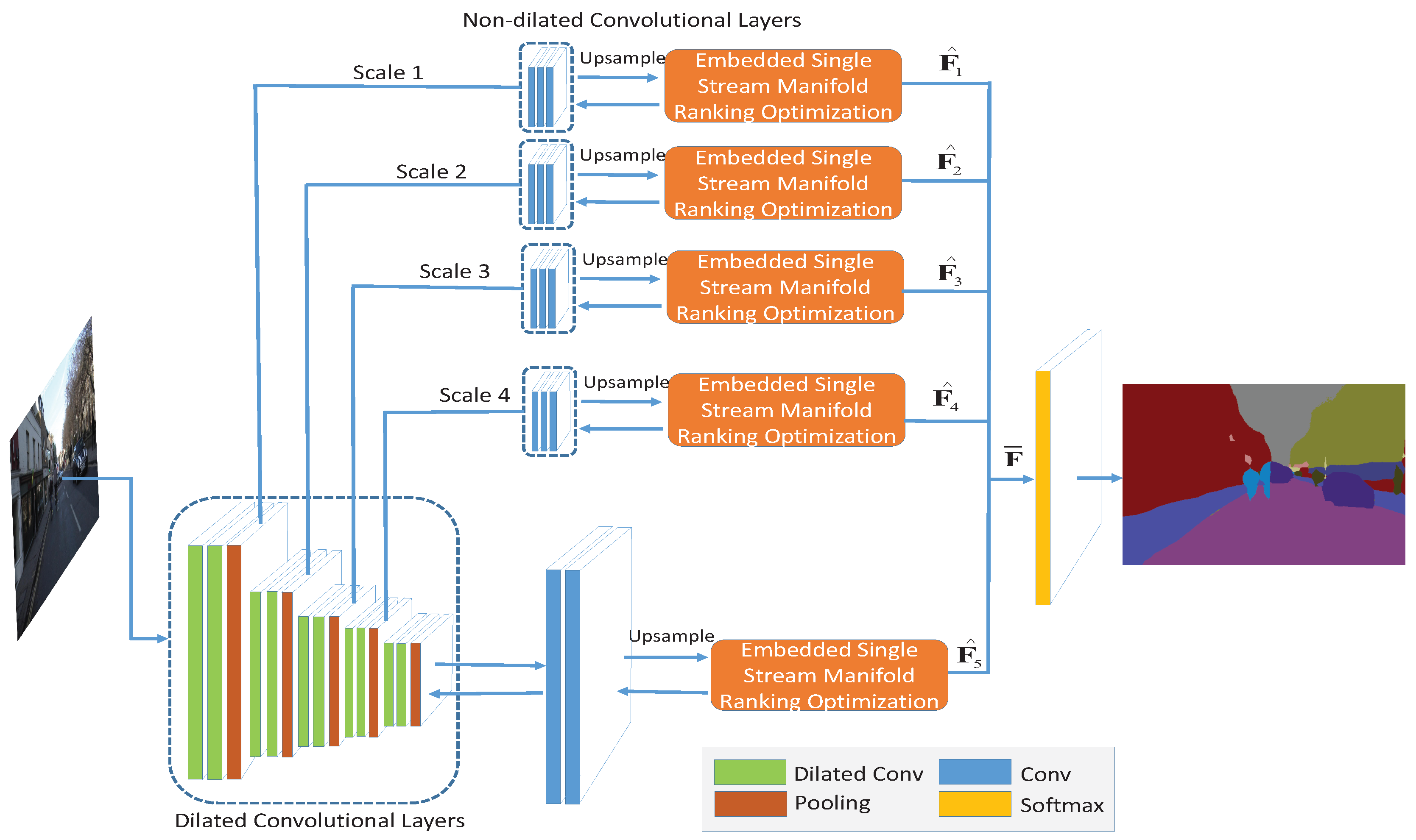
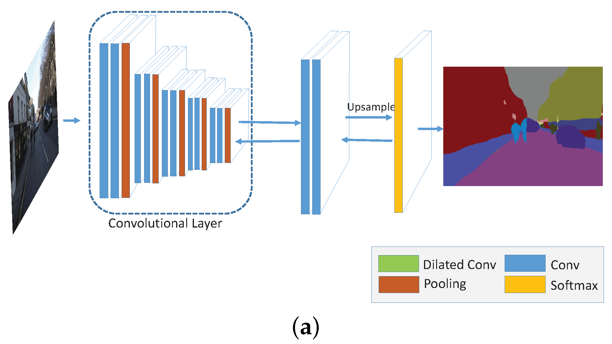
Numerous strategies without CRF optimization have been established to improve the semantic segmentation accuracy in the FCN or deconvolution manner, and each of them has its own superiorities [25,26,27,29,35,40]. In order to take these advantages, we propose a framework called dual multi-scale manifold ranking (DMSMR) network to estimate the predicted labels in an end-to-end fashion. In each scale, the dilated and non-dilated convolution layers are jointly optimized by MR. With the dual multi-scale contextual information, the combined results achieve competitive accuracy without any additional aides. An overview of our proposed approach is illustrated in Figure 1.
We conduct experiments on high spatial resolution remote sensing and close-range images to validate the effectiveness of the proposed approach. Both high spatial resolution remote sensing and close-range images are rich in details, such as texture and color information. The close-range images can be viewed as a special kind of high-resolution images and can guide us to find better CNN architectures to deal with high-resolution remote sensing images. In summary, the main contributions of our work are as follows:
(1) Multi-label MR graphical model for semantic segmentation. Unlike existing approaches that utilize the CRF as the post-processing or approximate inference in the discrete domain, we propose to model the MR method for semantic segmentation in a continuous domain. Our model is end-to-end optimization that can be linearly solved and guarantee a global optimal solution.
(2) Embedded feedforward single stream optimization method. In contrast to Gaussian graphical models, we propose an embedded single stream technique that requires only the Laplacian matrix obtained from pairs of vertices, which makes the gathering of the low-level cues as the contextual information more efficient.
(3) Dual multi-scale manifold ranking network. We adopt the multi-scale strategy to construct the dual-dilated and non-dilated networks and jointly optimize them with MR in a unified framework for semantic image segmentation. Our model is the first work to back propagate through manifold ranking and integrate it to deep learning architecture in the area of remote sensing.
2. Related Work
In the past decade, convolutional networks have been driving advances in object recognition. Therefore numerous semantic segmentation tasks have preferred to conduct dense prediction based on CNNs in both computer vision and remote sensing areas.
In [21,41,42], each semantic object is refined from region proposals by CNN features. In contrast to these instance-awarded methods, Mostajabi et al. [20] and Dai et al. [43] sought to preserve the shape information for dense labeling from superpixel-wise proposal segments. Unlike these approaches, Farabet et al. [44] trained on the entire image with a multi-scale strategy and labeled each pixel with the category of the object to which it belongs. A remarkable breakthrough was recently made by Shelhamer et al. [22]. In their approach, the contemporary classification networks are converted into fully convolutional networks (FCNs) and the fully connected layers in standard CNNs are viewed as convolutional layers with large receptive filed. Yu et al. [23] presented a dilated module to the FCNs to further broaden the receptive filed on the convolution layer. Instead of adopting the “convolution by pooling” schema in the classification task, they used a dilated rectangular prism on the convolution layer to preserve the receptive field. Similar strategies were proposed by Chen et al. [24,45] in the DeepLab framework. With the “hole” algorithm, a fast dense prediction is allowed on modern GPUs. More recently, Bearman et al. [46] exploited a point-wise annotation for semantic segmentation, which creatively makes a better trade-off between training annotation cost and accuracy. In the area of remote sensing, Camps-Valls and Romero et al. [47,48] proposed the use of greedy layer-wise unsupervised pre-training that learns sparse features for remote sensing image classification. Tschannen et al. [49] introduced a structured CNNs that employed Haar wavelet-based trees for identifying the semantic category of every pixel of remote sensing image. Piramanayagam et al. [50] further exploited a multi-path CNNs that support both true ortho photo and digital surface model (DSM) for land cover classification. Marcu et al. [51] presented a dual path, that is VGG-Net path and AlexNet path, to learn local and global representations of aerial images. Yuan et al. [52] also conducted a dual clustering approach to select optimal bands for hyperspectral remote sensing images. A few of these approaches are derived from basic FCNs model and utilize different strategies, such as multi-scale pyramid pooling, dilated convolution, dual-path representations and symmetric structures, to improve the inner stability of CNNs. Nevertheless, these networks still need to be properly initialized from pre-trained model or additional aides and may lack of contextual information.
As special extensions to basic FCNs, the symmetric encoder/decoder structures are further exploited by numerous recent approaches. The symmetric structures are able to delineate finer details of the upsampled output. In [27,53], Kendall and Badrinarayanan et al.presented a novel semantic pixel-wise segmentation architecture called SegNet. The architecture comprises an encoder that corresponds to the 13 convolutional layers in the VGG-16 [54] model and a decoder that maps the final features up to the full original image resolution. A similar schema was proposed by Hong and Hyeonwoo et al. [28,55]. The deconvolution network is composed of convolution and unpooling layers, thereby mitigating the limitations of the existing methods based on FCNs and handling the object in multi-scale space. Such symmetric structures were also applied to remote sensing image processing. Audebert et al. [56] exploited the symmetric encoder-decoder structure to detect, segment and classify different varieties of wheeled vehicles from aerial images. Huang et al. [57] further presented two symmetric encoder-decoder structures to fine-tune the networks from RGB and NRG bands. Audebert et al. [58] combined the SegNet with SVM to generate the geometrically corrected orthophoto. These symmetric structures reduce possible loss in the uppooling procedure of CNNs. However, these approaches may suffer from the bottleneck of GPU memory and contextual information embedding in terms of training remote sensing images.
To overcome the above issues, various recent approaches use discrete CRF models on top of CNNs. The CRF is an effective optimization method that can further boost the performance of semantic segmentation. By exploiting more contextual information, the rough segments are able to infer the relationship with their surround pixels. In [32], dense CRF [33,40] was proposed for the first time to improve accuracy by utilizing CRF as a post-process with more contextual information for fine predictions on top of CNNs. To make better use of contextual cues, Lin et al. [29] exploited an efficient “patch-patch” and “patch-background” schema to improve the performance by the CRF optimization framework. Unlike [24], Zheng et al. [25] introduced a mean-filed approximate inference for CRF that has the advantages of CNNs and CRF and is easily incorporated to the CNNs. Furthermore, Vemulapalli et al. [35] and Chandra et al. [26] proposed the use of simple Gaussian conditional random field (G-CRF) for the task of structured prediction. In [59], CNN features and hand-crafted features were combined to parse remote sensing images. Alam et al. [60] further introduced a framework that combined with mean-field CRF inference and performed superpixel-level labellings on remote sensing images. Sherrah [60] exploited the effectiveness of CRF post-processing approaches on top of CNNs and analyzed the major differences between close-range and remote sensing images in terms of contextual information. However, these methods either serve as a post-process or end up with mean-filed approximation and do not guarantee a global optimum.
Hence, we combine CNNs with the MR method, which guarantees a global optimum in a unified framework without additional aides. The multi-scale, dilated convolution strategies are also incorporated on top of CNNs to better delineate visual objects in remote sensing images. The MR method presented in [36,37,39] is an effective graph-based ranking method that aims to find the underlying cluster or manifold structure from the given datasets. For a query data, MR seeks to rank the neighborhood relevance to the query. Unlike the CRF, the optimal ranking solution is linearly solved by constructing the Laplacian matrix [61] from the neighbor contextual information, guaranteeing a global optimal solution in the continuous domain. Quan [62] et al. exploited such characteristics and utilized the MR based co-segmentation strategy to find the common objects contained in a set of relevant images. Wang et al. [63] presented an effective approach for salient band selection for hyperspectral image classification via MR. They put the band vectors in a more accurate manifold space and treats the salient band selection problem from a ranking perspective. Moreover, the MR method has been applied to estimate the status of many other complex low-level vision tasks, such as saliency detection [38,64], image retrieval [65,66] and visual tracking [67]. Considering that the semantic segmentation task also has a manifold structure, in which each pixel is first assigned several probabilities (ranking) that belong to the given categories (underlying clusters) and then the maximum probability is obtained from them, we apply the MR method embedded in CNNs to exploit the efficient global optimal solution to semantic segmentation. Combined with dilated, multi-scale strategies, the MR method, which can further establish the foundation of the dense prediction task in an end-to-end manner, is introduced into this field.
3. Manifold Ranking Formulation
The goal of graph based manifold ranking is to find the rank of a neighborhood relevance to the query node. Learning the objective function, which defines the relevance of neighbor nodes and query, is necessary to achieve this goal. In this section, we briefly describe the manifold ranking algorithm in a binary case and further extend it to multi-label situations that can be applied to the semantic segmentation task.
3.1. Binary Manifold Ranking
In [65], a binary ranking method was presented to exploit the manifold structure of the dataset. Given a set of data , a graph with vertices and edges can be built on the dataset. The weight between two vertices and connected by the edge is denoted by , which is commonly obtained by the Gaussian weighting function, that is . In addition, the degree of a vertex is given by . If we let as a ranking function that assigns each point two ranking scores , , and as a binary indication vector in which if and otherwise, then the normalized Laplacian matrix is computed as follows:
where , and each element in the normalized Laplacian matrix is given by
And the optimal ranking score vector is obtained by solving the following manifold ranking energy function associated with f:
where , and is the corresponding posterior probability for each point . The first term in the energy function is a data term that encodes the intrinsic structure of the given dataset, and the second term is a smoothness term that demonstrates the compatibility of the query data with its neighbors. By minimizing the energy function, we obtain the optimal ranking scores through the following close form
where , , , is the degree of the vertices, is the compatibility matrix as mentioned in Equation (1), is the unnormalized Laplacian matrix which is calculated as , is the regulation coefficient, and is the identity matrix. Given the optimal ranking score, the corresponding optimal indicator for each query point can be achieved by:
3.2. Multi-Label Manifold Ranking
In the previous subsection, we introduced the basic optimal manifold ranking solution to a binary label case in which each data has a unique binary indicator. In this section, we extend the binary MR solution to a multi-label situation and apply it to the semantic image segmentation task. As previously mentioned, given a set of pixels in an image , the semantic segmentation task aims to classify each pixel to one of the K possible classes. In other words, each pixel is assigned to the index of the K variables that has the highest ranking score. If we let denote the ranking score of the kth class, then the assigned label for pixel is
where k also stands for the index corresponding to the ranking score in each pixel.
Although our objective is to assign each pixel an optimal discrete label , we first find the optimal ranking vector and then obtain the optimal ranking score of each pixel in the continuous domain. Once we find the maximum ranking score for each pixel , we can easily assign each pixel a discrete label using Equation (6).
In order to compute the optimal ranking score vector for the multi-label situation, we extend the Equation (3) to the generalized energy function as follows:
where , and is the posterior probability vector for each pixel . The corresponding cost function in matrix form is
where and are the matrices accounting for the degree of the vertices and the compatibility for the multi-label case, denotes the unnormalized Laplacian matrix in a multi-label situation, is a diagonal matrix containing the regulation coefficients for the data term, and and are built from the ranking score vectors and , respectively.
The solution is optimal if the derivative of yields zero in the Equation (8). Specifically,
Therefore, the optimal solution to Equation (8) is
4. Deep Multi-Scale Manifold Ranking Network
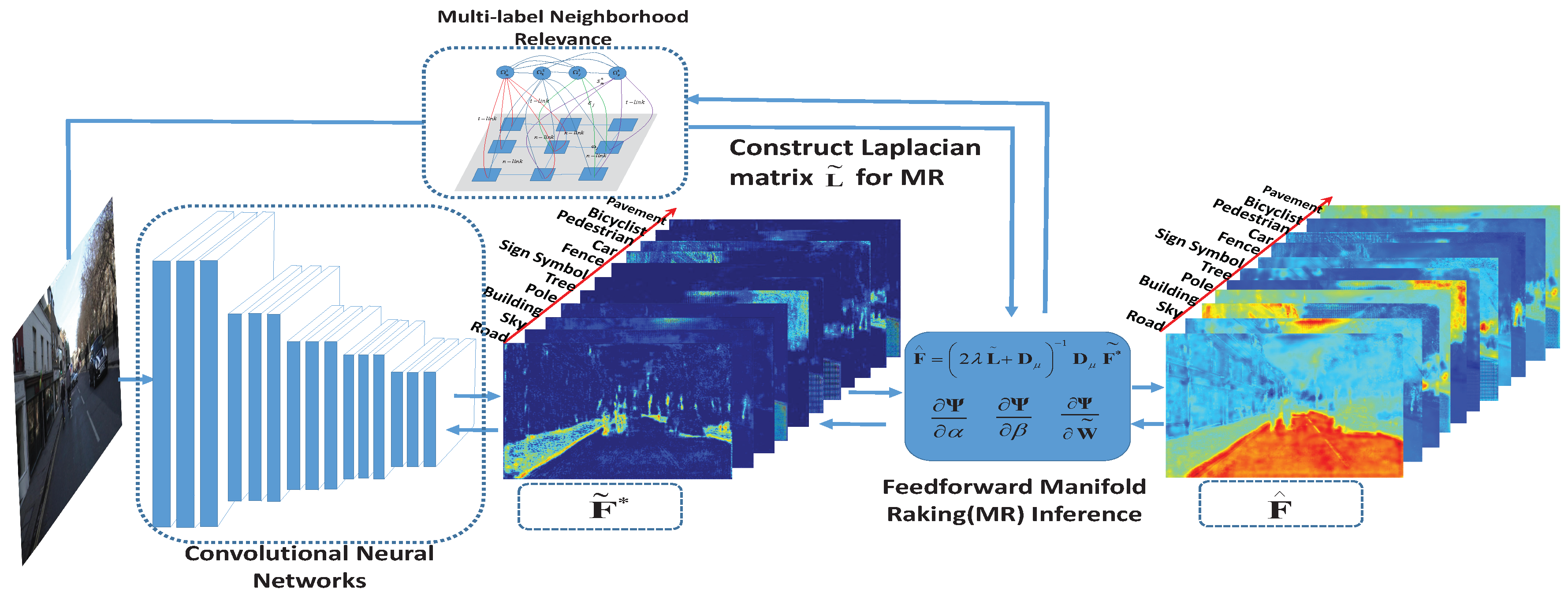
In order to incorporate the proposed multi-label manifold ranking algorithm into CNNs, we first embed the single stream manifold ranking method in a feedforward schema [20] into the network. Figure 2 shows how the MR optimization method is embedded to the single stream network. By exploiting the derivative of the learned parameters with respect to the loss function in the feedforward network, the required parameters can be trained in an end-to-end manner. Then, a DMSMR network is constructed, in which the dilated [23] and non-dilated networks are jointly optimized through the multi-scale feedforward manifold ranking method .
4.1. Embedded Feedforward Single Stream Manifold Ranking Optimization
Calculating the derivative of the learned parameters with respect to the loss is necessary to train the embedded multi-label MR network. In the following subsection, we describe the inference procedure for the manifold ranking algorithm in detail and describe the mathematical form of the derivatives.
4.1.1. Manifold Ranking Inference
As previously mentioned, the key to manifold ranking is seeking the neighborhood relevance to the query. For the semantic segmentation task, we model the neighborhood relevance, that is, the smoothness term in Equation (7), as follows:
where the first kernel (Here the notation “kernel” refers to Potts model.) measures the color likelihood nearby and the second term weights the spatial position correlation. and are the smoothness coefficients. and are the image intensities, and denote the position of neighbor pixels, and are the degrees of nearness and similarity, respectively.
Our formulation is based on the energy hypothesis proposed in Equation (7), and the inference to this energy function for semantic image segmentation is provided by Equation (10). Given the smoothness relationship in Equation (11), we can easily setup a single stream manifold ranking neuron from the compatibility matrix . We only need to learn the smoothness coefficients , and the compatibility matrix in a single stream rather than two streams in the network, that is, the unary and pairwise streams presented in [26,29].
In our work, the preceding parameters are determined by the stochastic gradient descent (SGD) algorithm [70]. The loss between the predicted label in Equation (6) and the ground truth y is indicated by . Therefore, the derivative of with respect to can be represented as
In our experiment, we use softmax loss as the loss function. In order to learn the smoothness coefficients , and compatibility matrix via SGD, the derivatives of these parameters, that is, , , , for loss function are necessary.
4.1.2. Derivative to Smoothness Coefficients
The derivative of loss function in terms of smoothness coefficients , can be obtained by the chain rule shown below:
where is the delta function for the derivative result of with respect to , and are the smoothness kernels.
4.1.3. Derivative to Compatibility Matrix
Similar to the derivative to smoothness coefficients, the derivative of the compatibility matrix with respect to the loss function can be represented as
where is the linear solution to manifold ranking energy function in Equation (8), ⊗ denotes the Kronecker product, and and represent the same as those in Equation (14).
4.2. Dual Multi-Scale Manifold Ranking Network
The recent works [23,26,27,28] shows that the CNNs have a remarkable capacity to implicitly represent a feature in a multi-scale space. The capacity of CNNs to find objects is dramatically improved by training the dataset with varying kernel sizes or pooling rates (i.e., in an atrous spatial pyramid pooling (ASPP) [24] schema). Meanwhile, the dilated rectangular prism of convolution layers [23] is a natural choice for boosting the performance and broadening the receptive field in each layer.
In our proposed network, we use a dual approach to handle the scale variability for the semantic image segmentation task. On the basis of the work presented in [71], the dual approach aims to minimize the residual produced by dilated and non-dilated networks in each scale. Let be a discrete function that denotes the optimized ranking score with scale factor of l in a given convolutional layer and be the dilation filter in this layer. The objective function for the DMSMR network can be represented as follows:
where denotes the objective function that measures the output difference between the dilated and non-dilated layers, is the input obtained from the non-dilated convolutional layer with a scale factor of , ∗ is the dilated convolution operator, and and represent the weights for the dual outputs, that is, the dilated output and the non-dilated output , respectively. The objective function in Equation (16) models how to combine the dilated and non-dilated layers in the l scale. The final results from all the scales are fused by the following equation:
where is the fusion result for the multi-scale space, and N is the total number of scales. Figure 1 illustrates the corresponding relation.
5. Experiments
We have devised two groups of experiments on high resolution datasets, including close-range images (PASCAL VOC dataset and CamVid dataset) and remote sensing images (ISPRS Vaihingen dataset and EvLab-SS dataset), to validate the effectiveness of our model and find the approach that can be potentially applied to remote sensing image processing. For fair evaluation, the first group, which includes the PASCAL VOC dataset [72] and ISPRS Vaihingen dataset [73], is designed for comparison with a few recent state-of-the-art methods whose results are publicly available online. In this group, we evaluate our model by submitting the results to the server, wherein the ground truth of testing images are not available to all researchers. The second group, which includes the CamVid dataset [68,69] and the EvLab-SS dataset (See Section 5.2.2), is used to evaluate the capacity of the proposed DMSMR approach by comparing the methods that employ only one of the three strategies, namely, multi-scale convolution (MS), broader receptive field (Dilated) and MR optimization (MR-opti) approaches. The detailed structures of the network with different strategies are explained in the Appendix (See Figure A1 and Table A1).
In our DMSMR model, the first five blocks are developed from the standard VGG-16 [54] structures, which comprise convolutional and non-dilated convolutional layers. The dilation kernel sizes are 6, 4, 2, 2, and 1 pixels. For each scale, the pooling layer is followed by the non-dilated layers, which comprise three convolutional layers. The parameters of our implementation are shown in detail in Table 1. The dilated and non-dilated layers are optimized with single stream manifold ranking algorithm and fused by Equation (17). The structure is illustrated in Figure 1. In the table and figure, the “ReLU” active function [74] is implicitly employed in each convolutional layer. In our model, all layers are randomly initialized without using the pre-trained VGG-16 model. The hyper-parameters, such as learning rate, momentum and weight decay, are confirmed via cross validation. The entire net is trained in an end-to-end manner using SGD algorithm. and in Equation (11) are both set to as in [32] in our experiments.
The proposed architectures are implemented using Caffe [75] in a Win7 x64 platform running on an Intel I7-4790 CPU @ 3.6 GHz with a single GeForce GTX 1070 (8 GB RAM). Our model requires only 5523 MB of GPU memory. The source code is implemented with C++ and the model is publicly available at http://earthvisionlab.whu.edu.cn/zm/SemanticSegmentation/index.html.
5.1. Experiment on Close-Range Dataset
As a special kind of high resolution image, close-range imagery is rich in details. Many of the recent breakthroughs [12,13,14,49,50,76] in the remote sensing area used pre-trained models on this kind of high resolution images. We adopt the PASCAL VOC dataset [72] and the CamVid dataset [68,69] for training and testing and to evaluate the proposed approach on close-range images. The PASCAL VOC dataset is a golden standard measurement for semantic segmentation evaluation. Meanwhile the CamVid dataset comprises a small number of training images, and is a reasonable choice for evaluating the intrinsic capacity of the network that employs different strategies.
5.1.1. Evaluation on PASCAL VOC
The PASCAL VOC 2012 segmentation dataset comprises 20 object classes and one background class with 1464, 1449 and 1456 images for training, validation and testing, respectively. In our experiment, we use the extra annotations provided by [77], thus obtaining a total of 10582 augmented training images [77,78]. For our model, we resize the images to pixels as in DeepLab model [24] and evaluate the model by remotely submitting the predictions to the test server (Our result on PASCAL VOC dataset is available at http://host.robots.ox.ac.uk:8080/leaderboard). The evaluation metric is the standard Intersection-over-Union (IoU) averaged across the 21 classes. In our experiment, we train the model with the initial learning rate, momentum and weight decay 1e-9, and , respectively. The momentum and weight decay terms are utilized as suggested in FCNs framework [22]. In addition, the learning rate is confirmed via cross validation. The initial parameters for smoothness coefficients and are set to 3 and 5, respectively. The drop-out layers are removed in our proposed approach. Our network converges after 60,000 iterations with a mini-batch size of 8.
Numerous methods have been applied to the PASCAL VOC 2102 dataset and achieve the high accuracy. However, the complexity has been increasing due to the gradual addition of aides, which unfortunately does not reveal the true performance of the deep architecture as stated by Kendall et al. [27]. Our work in this benchmark do not aim to obtain the top score using additional aides, such as CRF post-processing [24], region proposal [28], multi-stage inference [25], and pre-trained model from other dataset (e.g., Microsoft COCO [79]). Instead, we seek to improve the performance by applying three main strategies, which include multi-scale convolution, a broader receptive field, and a single stream MR optimization method, to jointly upgrade the intrinsic structure of the network. The multi-scale strategy has the advantage of deep architecture because the potential scale is implicitly expressed by a pooling layer in the CNN. The broader receptive filed is captured by a dilated operation [28], thus preventing the loss of resolution. By contrast, the feedforward single stream MR optimization method allows obtaining the optimal solution without the complicated inference procedure and can be trained in an end-to-end manner. Though we embed the feedforward MR optimization algorithm into the network, the optimal solution can be solved linearly rather than in a multi-stage inference schema.
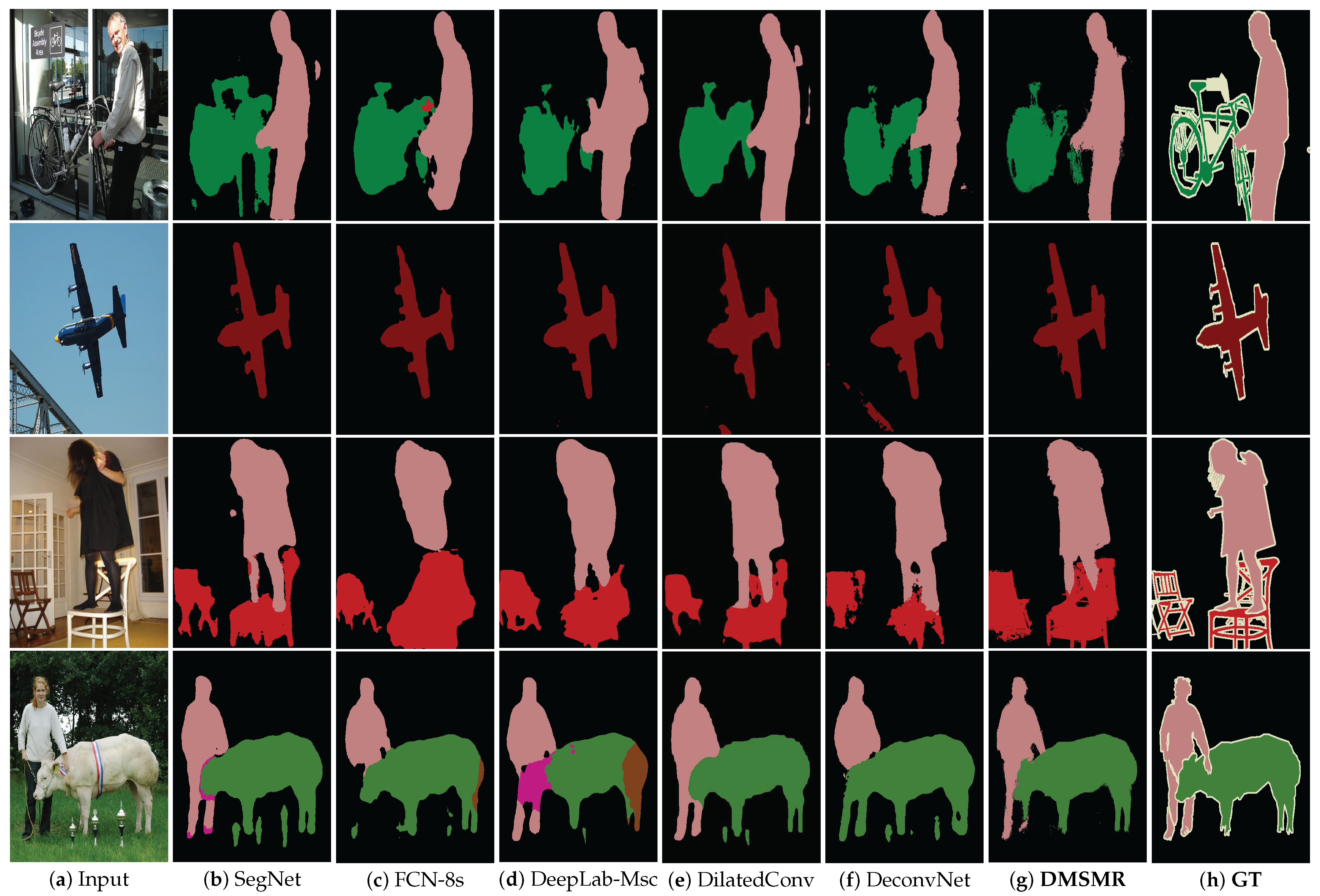
Table 2 presents the results of the comparison to recent methods, and a few of the corresponding intuitive results are depicted in Figure 3. In the table, we compare our method with several models that can be potentially applied to remote sensing area. We choose the listed models rather than all top scored approaches for the following reasons. First, the model should utilize as less additional aides as possible. Additional aides can hide the true performance of a network and are not easily transplanted to remote sensing application. Several models on the table, such as FCN-8s [22], DeconvNet [28] and SegNet [27], have been applied to process remote sensing images. Second, the selected model needs to be tested on PASCAL VOC 2012 server and does not repeat with previous methods. Algorithms, such as DeepLab [24], CRF-RNN [25], DilatedConv [28], and G-CRF [35], are milestones on PASCAL VOC 2012 benchmark and satisfy such requirements. Third, training the model is not too much time consuming, especially when dealing with remote sensing images, which are usually bigger than close range indoor/outdoor images. The recent state-of-the-art approach, such as RefineNet [80], employs ResNet-101 structures that may suffer from high GPU consumption and need MS-COCO dataset support. In the area of remote sensing, however, we do not have the large number extensions of labeled samples for training.
In the Table 2, the proposed DMSMR performs significantly (averaged approximately eight points) better than the similar methods without additional aides (methods without qualifying comments in Table 2). This is because our method is composed of the dilated, multi-scale strategies and has characteristics that complement to a few basic networks, such as SegNet [27], dilated convolutional network [28] and DeepLab-Msc [24]. Compared to recent methods, such as CRF-RNN [25] and G-CRF [35], our method achieves a similar score by optimizing with a single stream MR algorithm in an end-to-end manner. However, our approach does not require multi-stage inference or training two streams (i.e., unary term and pairwise stream, with unary initialized by other networks). Furthermore, some approaches, such as DeepLab [24], have a worse result when they do not use all of the additional aides with a pre-trained model. However, our model yields superior results without these pre-trained weights.
5.1.2. Evaluation on CamVid
CamVid dataset [68,69], which is captured from high-definition (HD) video sequences with high quality, is designed for the road scene understanding. However, a relatively few number of images exist for training purpose. The dataset comprises 367 training images, 101 validation images and 233 testing images. The challenge data contains 11 semantic object classes which are downsampled to pixels.
The overall training parameter settings for this dataset are as follows. The learning rate, momentum and weight decay are set to 1e-3, and , respectively. The momentum and weight decay terms are utilized as suggested in FCNs framework [22]. In addition, the learning rate is confirmed via cross validation. The proposed network is trained at the default resolution of with a mini-batch size of 2. The initial values for and are set to 3 and 5, respectively, through cross validation. Our network converges after 40,000 iterations.
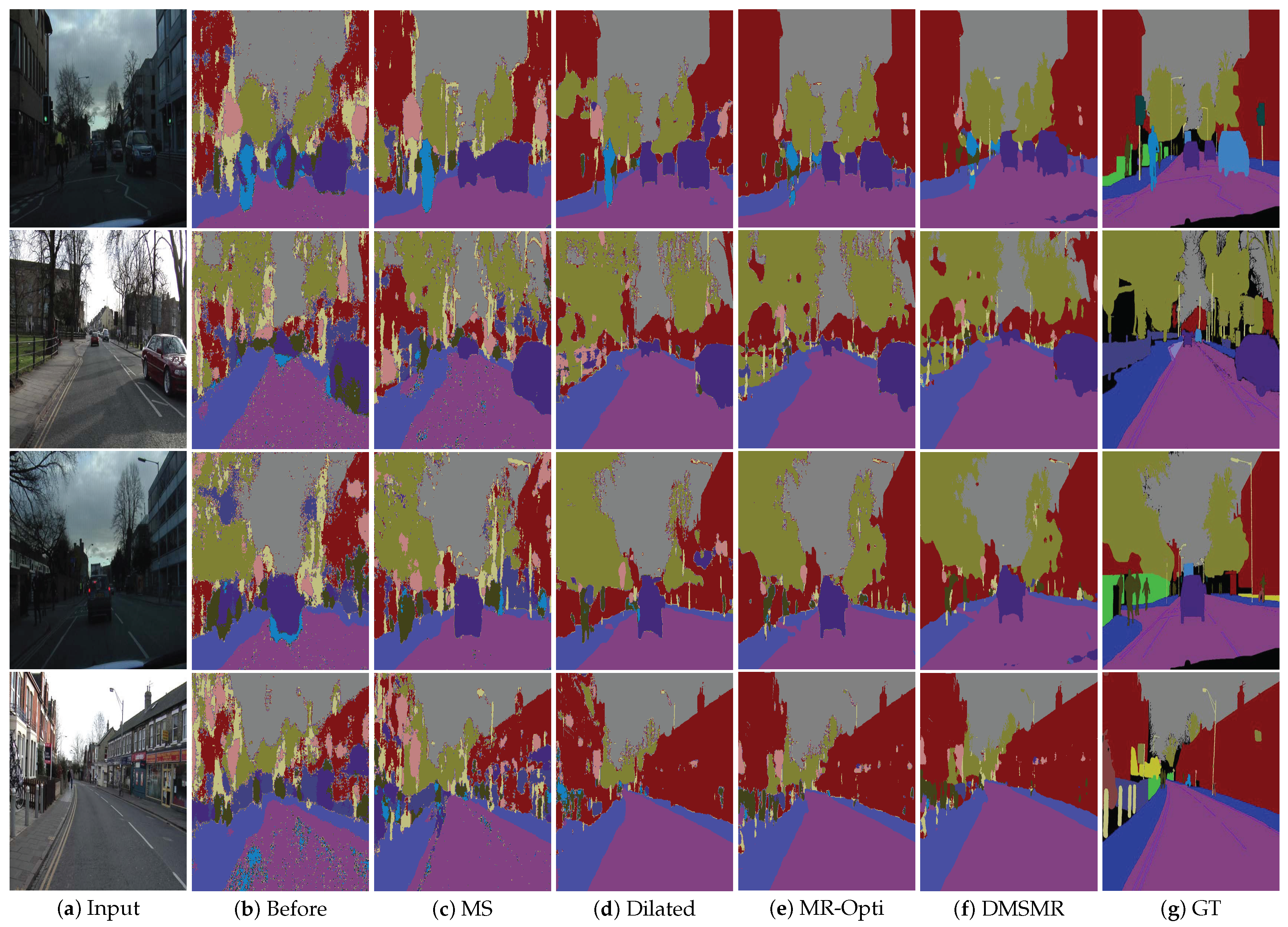
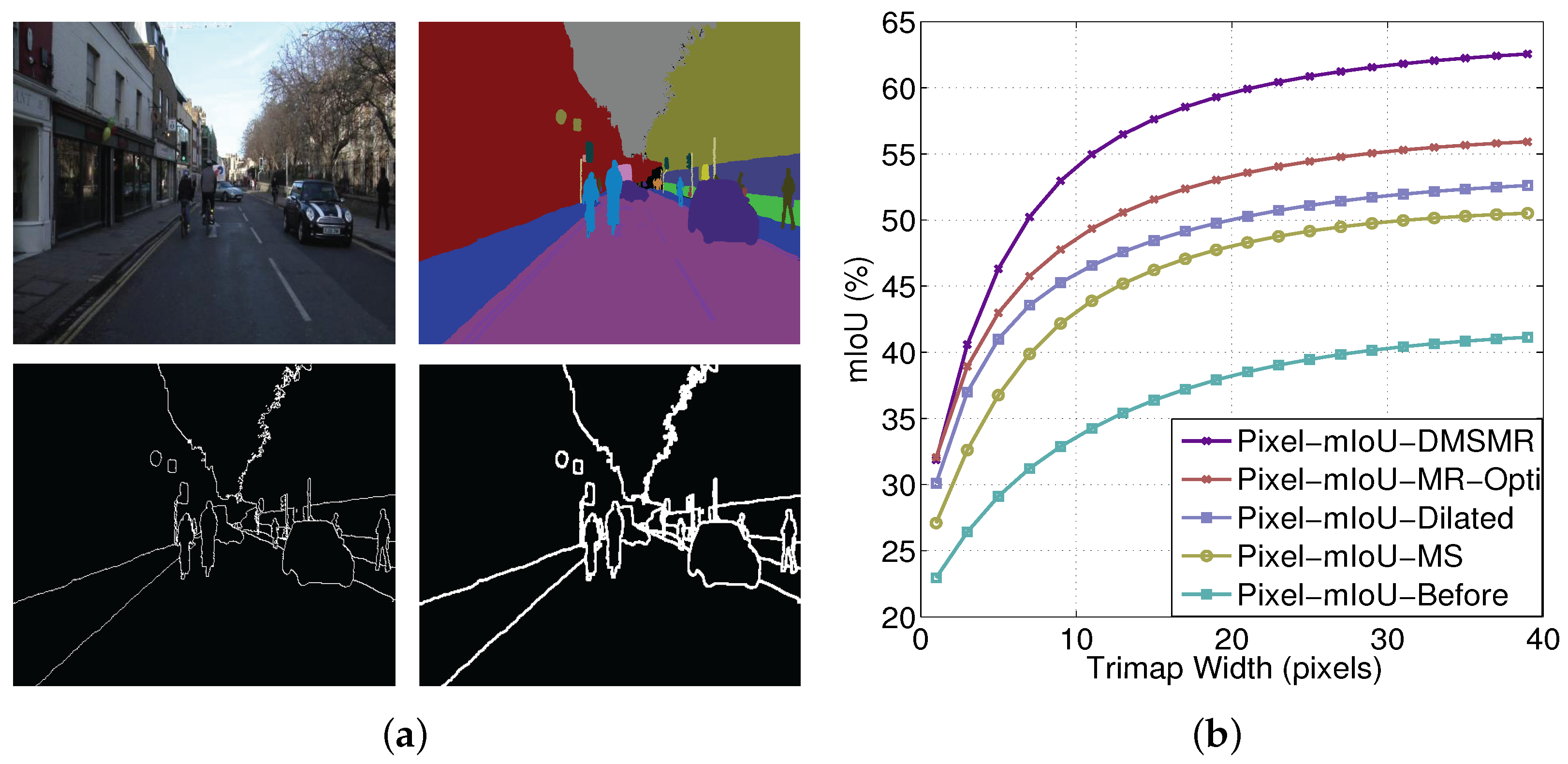
We employ the pixel mean intersection over union (mIoU) measurement with respect to the band width around the object boundaries as in [24] on the CamVid benchmark to analyze the expressive power of the proposed DMSMR network. The experimental results are illustrated in Figure 4. The comparisons between the DMSMR approach and the networks employing different strategies are reported in Table 3. We also analyze the accuracy change with respect to boundary in Figure 5. As shown in Figure 5a, we consider a narrow band, that is, trimap [81] boundary, on CamVid dataset. A trimap divides an image into three regions of foreground, background and unknown. Figure 5b shows boundary accuracy as the trimap width is varied. In this experiment, we set the same parameters as those in the DMSMR model but with different strategies as previously stated. The three strategies, namely, multi-scale convolution (MS), broader receptive field (Dilated) and manifold ranking optimization (MR-Opti) approaches, are utilized for comparison. Obviously, different strategies yield different performance for each of the classes. The MS and Dilated approaches help boost the performance in the situation where color and texture are uniformly distributed. In addition, the MR-Opti achieves a score that is approximately 2.5% better than those of the MS and Dilated methods because more contextual information are considered. The results demonstrate that the combination of MS, Dilated and MR-Opti approaches is possibly a better approach for semantic segmentation task on close-range images. Figure 5 shows that improving the recognition of pixels around the boundary helps delineate the object because the smoothness potentials of the correctly detected pixels increase. Additionally, as can be seen from Table 3, the DMSMR method outperforms the approaches that employ only one strategy, indicating that the DMSMR approach can improve the semantic segmentation result further by combing these strategies in close-range situations.
5.2. Experiment on High Resolution Remote Sensing Dataset
Compare to the close-range imagery, high resolution remote sensing images have a few special features, which are different from that of commonly encountered indoor/outdoor close-range images in the area of computer vision. High resolution remote sensing images are large and contain a potentially-unlimited scene context (i.e., the road could possibly pass through the entire image). In addition, the object scale on high resolution images dramatically varies when employing the training dataset captured from different satellites (i.e., GF-1 with spatial resolution 2.1 m, QuickBird with spatial resolution of 0.6 m), whereas the close-range images do not. In the following experiments, we adopt two kinds of benchmarks: the ISPRS 2D Vaihingen dataset and EVLab-SS dataset. The ISPRS 2D Vaihingen benchmark is a well-known high resolution aerial imagery semantic labeling database, whose spatial resolution is 0.9 cm with uniform color and texture distributions. The EVLab-SS benchmark, which is designed for evaluating the semantic segmentation results on remote sensing imagery, contains the images captured from different platforms (both aerial and satellite images are included) with different types of spatial resolutions (ranging from 0.1 m to 2 m). In addition, the images vary in color, gradient, and texture.
5.2.1. Evaluation on Vaihingen Dataset
The Vaihingen dataset comprises 6 classes with 33 image tiles, out of which 16 are fully annotated (tile numbers 1, 3, 5, 7, 11, 13, 15, 17, 21, 23, 26, 28, 30, 32, 34 and 37). The dataset is cropped from an aerial orthophoto mosaic (GSD 9 cm) with three spectral bands (i.e., red, green and near-infrared bands) that are rich in detail. The categories to be classified for each pixel are impervious surfaces, buildings, low vegetation, trees, and cars. In our experiment, we randomly sample 2932 patches of pixels from annotated images by sliding window. All patches are reserved for training. For the objective evaluation of the proposed approach, we submit the predicted results to the organizers who keep the ground truth.
The training procedure is performed with the SGD algorithm. The mini-batch size is set to 8, and each batch contains the cropped images that are randomly selected from training patches. These patches are resized to pixels. We employ the “poly” learning policy, and the base learning rate is 1e-7 with the power of . The momentum and weight decay are set to 0.9 and 0.0005, respectively, as recommended by Krizhevsky et al. [82]. Smoothness coefficients and are set to 3 and 5, respectively. Our network converges after 50,000 iterations on this benchmark.
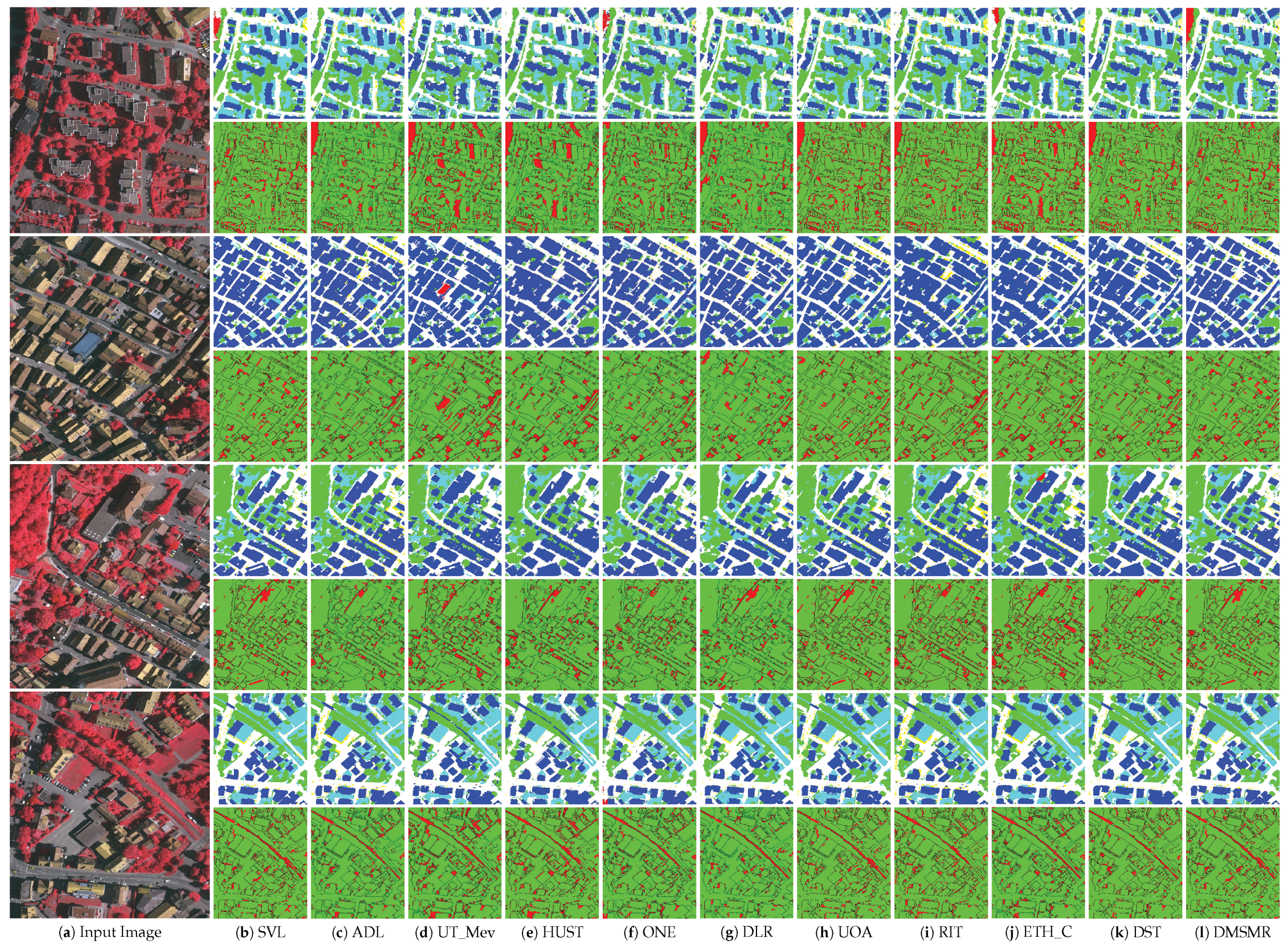
The experimental results on the Vaihingen testing images are available online (Our result on Vaihingen dataset is available at http://ftp.ipi.uni-hannover.de/ISPRS_WGIII_website/ISPRSIII_4_Test_results/2D_labeling_vaih/2D_labeling_Vaih_details_Ano2/index.html). Figure 6 visualizes the comparative results on a few testing images (tile numbers 2, 4, 6 and 8) with different methods. The quantitative evaluations of the corresponding state-of-the-art methods and our proposed network architecture are reported in Table 4. In this experiment, we employ the averaged F1 score and the overall pixel-wise accuracy as the evaluation metrics.
Figure 6 presents the visual comparison of these approaches. It can be seen from the error map that the CRF post-processing method (ADL [59] and HUST [83]) indeed helps improve the performance. Nevertheless, the upper left corner of the error map in the first row shows that even if the CRF post-processing method is employed, more incorrectly classified pixels will exist if the initial predictions are poorly provided. In Table 4, we compare our approach with the methods using additional aides, such as the VGG-16 pre-trained model [29,76,84], digital surface model (DSM) [49,85,86], and the CRF post-processing [59,83]. We also compare our approach with traditional feature based methods [87]. Recent advances in the area of computer vision have shown that very deep networks can improve the semantic segmentation accuracy [27,54]. Therefore, our DMSMR approach reasonably outperforms the “SVL” method by approximately in overall pixel-wise accuracy and on global F1 score. Although additional aides help improve accuracy, they are not the core to segmentation engine [53]. Our networks do not need these aides but achieve competitive scores compared with these approaches. For the fine-tuned networks from the pre-trained VGG-16 model (ONE [84], DLR [76], UOA [29], RIT [50]), their performances are not always steady compared to that of the proposed DMSMR approach. Our overall accuracy varies approximately 0.1% (see Ano (Ano is available at http://ftp.ipi.uni-hannover.de/ISPRS_WGIII_website/ISPRSIII_4_Test_results/2D_labeling_vaih/2D_labeling_Vaih_details_Ano/index.html) and Ano2 in the ISPRS leader board. Ano and Ano2 are initialized with the same hyper-parameters, but the weights and biases terms are randomly initialized.) when tested on this benchmark. This is mainly caused by uncertainty of weights when trying to transfer the VGG-16 classification networks into semantic segmentation task. The dense prediction problem, such as semantic segmentation, is structurally different from image classification [23]. Thus these performances are not as stable as expected. Our approach somehow utilizes the dual-dilated and non-dilated convolutional layers to prevent such instability.
5.2.2. Evaluation on EvLab-SS Dataset
The EvLab-SS benchmark (EvLab-SS dataset can be downloaded from our website http://earthvisionlab.whu.edu.cn/zm/SemanticSegmentation/index.html.) is designed for the evaluation of the semantic segmentation algorithms on real engineered scenes, which aims to find a good deep learning architecture for the high resolution pixel-wise classification task in remote sensing area. The dataset is originally obtained from the Chinese Geographic Condition Survey and Mapping Project, and each image is fully annotated by the Geographic Conditions Survey (NO.GDPJ 01—2013) [89] standards. The average resolution of the dataset is approximately pixels. The EvLab-SS dataset contains 11 major classes, namely, background, farmland, garden, woodland, grassland, building, road, structures, digging pile, desert and waters, and currently includes 60 frames of images captured by different platforms and sensors. The dataset comprises 35 satellite images, 19 frames of which are captured by the World-View-2 satellite [90] (re-sample GSD 0.2 m), 5 frames are captured by the GeoEye satellite [91] (re-sample GSD 0.5 m), 5 frames are captured by the QuickBird satellite [92] (re-sample GSD 2 m), 6 frames are captured by the GF-2 satellite [93] (re-sample GSD 1 m). The dataset also has 25 aerial images, 10 images of which with spatial resolution of 0.25 m and 15 images have a spatial resolution of 0.1 m. In our experiment, we divide the dataset into 37 frames for training, 8 frames for validation, and 15 frames for testing. We produce the training dataset by applying the sliding window with a stride of 128 pixels to the training images, thereby resulting in 48,622 patches with a resolution of pixels. Similar methods are utilized on validation images, thus generating 13,539 patches for validation. The Garden class, which is reserved for validating the expressive power of CNNs in real scenes, is absent in our validation images.
In the training procedure, each iteration comprises a feed-forward pass in which the model weights are adjusted by the SGD algorithm. Each training patch image in a batch is resized to pixels. The mini-batch size is set to 12 and the corresponding training patches are randomly selected. We employ the “poly” learning policy and start with a learning rate 1e-7 with the power of . Smoothness coefficients and are set to 3 and 5 in our experiments, respectively. The momentum and weight decay are set to 0.9 and 0.0005, respectively, as recommended by Krizhevsky et al. [82]. Our network converges after 70,000 iterations on this dataset. In the following experiments, we set the same learning parameters for the methods employing only one strategy (MS, Dilated or MR-Opti) as the DMSMR approach.
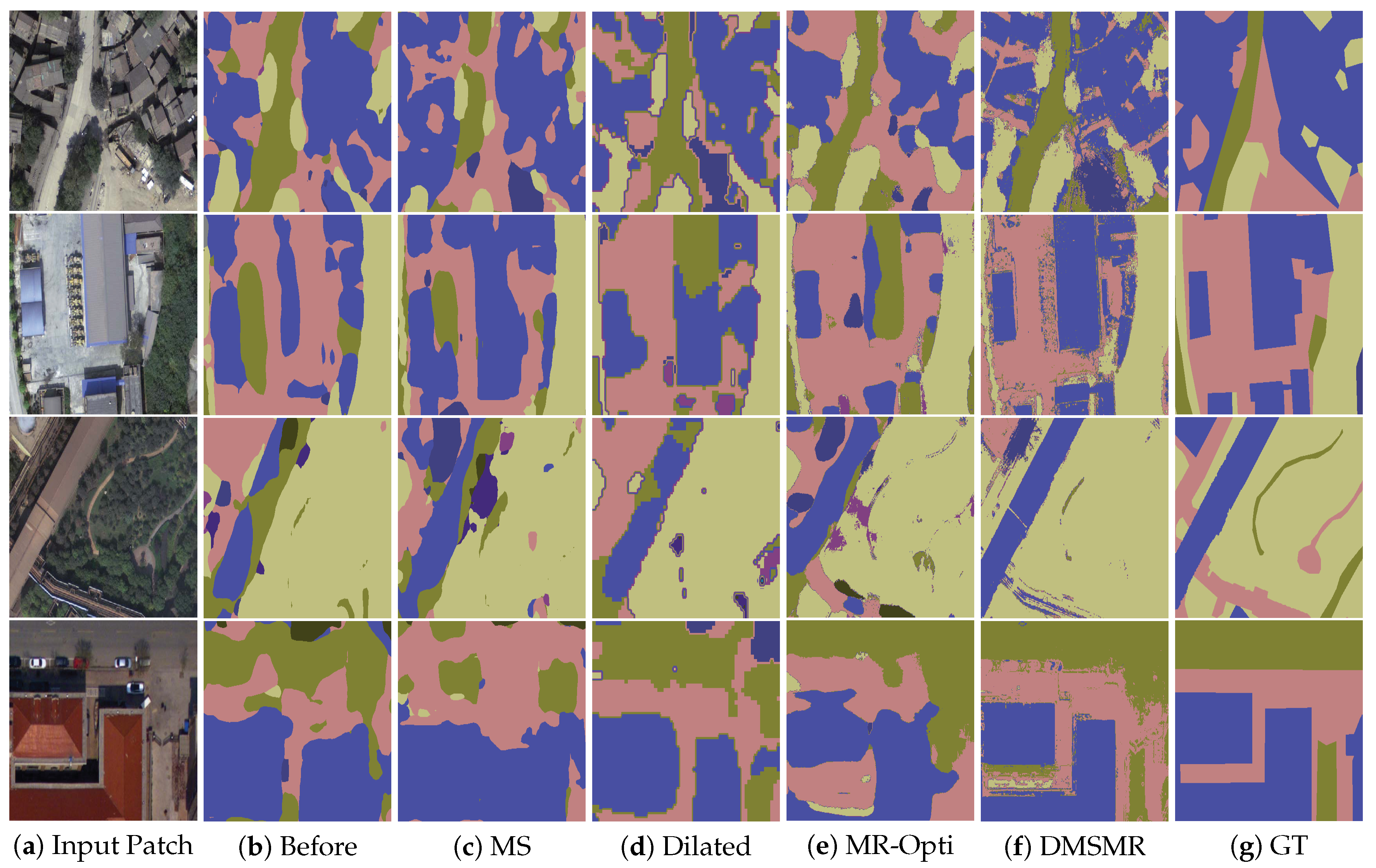
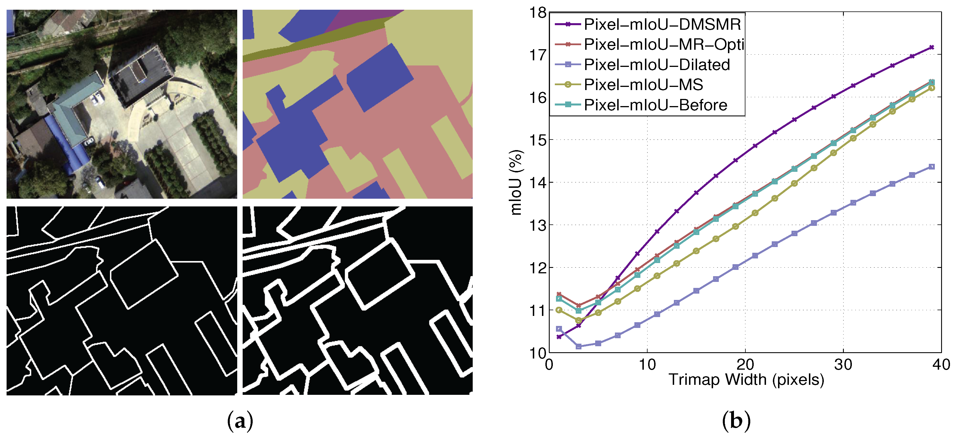
Figure 7 is the visualization of the results on the validation patches with different methods. Figure 8 illustrates the comparative results of employing different strategies with respect to the varying trimap band width. Quantitative results are shown in Table 5. In our experiments, we adopt the overall pixel-wise accuracy and mean intersection over union (mIoU) measurements to evaluate the effectiveness of different approaches.
Compare to the 2D Vaihingen dataset provided by the ISPRS organization, the EvLab-SS dataset is inconsistently distributed in terms shape, color, and texture. The resolutions of the images captured from different sensors are dramatically varying. The buildings, roads and other classes are not obtained in the same scale. Therefore, the EvLab-SS dataset poses more challenge to researchers. It intuitively can be seen from Figure 7 that the DMSMR method can better delineate the boundary of an object. The results demonstrate the superiority of the combination of multi-scale (MS), broader receptive field (Dilated), and manifold ranking optimization (MR-Opti) strategies, which can more accurately classify each pixel with varying spatial resolutions. Figure 8 shows that although the mIoU score of the proposed DMSMR approach is relatively low with a small trimap width, it has become increasingly stable and competitive. By contrast, the mIoU scores of the MS, dilated, and MR-Opti approaches are unstable, even decreasing with a few small trimap widths. The main reason attribute to this phenomena is that the spatial resolution is different in the training patches, which may be ignored by only employing one strategy. In Table 5, the special class (Garden) is detected as 0.0% in all approaches, indicating that these methods can preserve the intrinsic nature of CNNs well. For the real engineered remote sensing data, the Dilated approach does not appear to boost performance and decreases in overall accuracy and mean IoU by approximately 2.96%, 2.32%, respectively. This can be attributed to the numerous inhomogeneous objects in the training patches. For example, the road and buildings may not be completely covered in a single patch, which renders training with dilation operations in some layer meaningless. Although the MR-Opti approach improves the overall accuracy by approximately 4%, this approach may disregard a few classes, such as the Desert and Waters, due to insufficient contextual information with varying illumination and color. However, the MS approach retains more contextual information in each scale space but still suffers from the optimization problem in each scale, resulting in 0.8% decrease in overall accuracy. Notably, the proposed DMSMR approach can take the superior features of these strategies and overcome the drawbacks, achieving approximately 5% and 1% improvements in overall accuracy and mIoU score under the condition of limited training images and varying spatial resolutions.
6. Conclusions
In this paper, we present a DMSMR network for semantic image segmentation in a continuous domain. By extending the binary manifold ranking (MR) algorithm to a multi-label case, the assignment of a discrete label to each pixel can be linearly solved and a unique global optimum can be guaranteed. In addition, with the single stream MR method embedded into CNNs in a feedforward schema, the required parameters can be trained in an end-to-end manner. Furthermore, we propose to utilize dilated and non-dilated networks, which form dual layers to jointly optimize the results from the single stream manifold ranking network rather than on two separate streams, that is, unary and pairwise streams. Combined with multi-scale (MS), broader receptive field (Dilated) and manifold ranking optimization (MR-Opti) strategies, the proposed DMSMR network enables training without additional aides, such as multi-stage inference, region proposals, VGG-16 initialization, digital surface model (DSM) and CRF post-processing. Two groups of experiments on close-range and remote sensing high resolution datasets are designed to evaluate the performance. When discriminatively trained by submitting the results to the server on PASCAL VOC and ISPRS Vaihingen benchmarks, the proposed DMSMR network can achieve competitive results without additional aides compared to recent methods. Our experiments on publicly available datasets, including CamVid and EvLab-SS datasets, demonstrate the superior capacity of the proposed DMSMR approach over the methods that employ only one strategy. For the real world application in remote sensing, the combined strategy steadily boosts the performance even under limited training images and the varying spatial resolutions.
Nevertheless, the proposed approach may be further improved in the following ways. First, more prior information, such as orientation and texture, is expected to be integrated into the smoothness term in the multi-label manifold ranking objective function to delineate the visual objects with varying illumination and spatial resolution. Second, the generative adversarial nets [94,95,96] (GAN) can be introduced to boost the performance by combining the adversarial term in the loss function with the limited number of training images. Third, model parallelism should be investigated when incorporating more prior knowledge to our model. For example, buildings and roads are the salient objects in remote sensing images that can guide the semantic contextual information. The prior information might be parallel-trained in a distributed system. Finally, the superpixel segmentation can be applied as a pre-processing step to reduce the number of optimization elements in the proposed multi-label MR graphical model.
Acknowledgments
This work was partially supported by the National Key Research and Development Program of China (Project No. 2016YFB0501403) and National Natural Science Foundation of China (Project No. 41371401 and 91438203). The authors would like to thank Jiasi Yi and Yun He from Earth Vision Laboratory, School of Remote Sensing and Information Engineering, Wuhan University for designing the work flow to produce the EvLab-SS benchmark. The author would also like to thank the group of undergraduates from School of Remote Sensing and Information Engineering, Wuhan University for producing the EvLab-SS dataset.
Author Contributions
Mi Zhang designed the DMSMR network and performed the experimental analysis. He also wrote the paper. Xiangyun Hu guided the algorithm design, initiated the EvLab-SS dataset production and revised the paper. Shiyan Pang help organize the paper. Like Zhao, Ye Lv and Min Luo contributed to the design of project homepage and edited the manuscript.
Conflicts of Interest
The authors declare no conflict of interest.
Appendix A
In this section, we derive the rule of weights updating for learning the parameters mentioned in the paper and detailedly depict the implementation structures of the networks, which include the networks before and after employing the multi-scale (MS), dilated convolution (Dilated), and manifold ranking optimization (MR-Opti) approaches.
Appendix A.1. Learning Parameter α and β
To compute the term in Equation (13), we apply the chain rule through the following equation:
where , , , and are the symbols that have the same meaning as previously mentioned. is the simplified representation of the smoothness term in Equation (7), which is specifically denoted by
Since the term is equal to delta function , the term is equal to the identity matrix, the term and are obviously represented by and . The derivative of , with respect to are obtained by the following form:
Appendix A.2. Learning Compatibility Matrix
Similar to the derivative of smoothness parameters and , the derivative of compatibility matrix with respect to can be denoted by:
As discussed in the main paper, the optimal solution to the multi-label manifold ranking method is achieved by the following matrix form:
From Petersen et al. [88], we recall that the derivative of the inverse of matrix with respect to is
For the preceding term , the corresponding matrix form can be represented by:
Therefore, the derivative of with respect to is
Appendix A.3. Network with Different Strategies
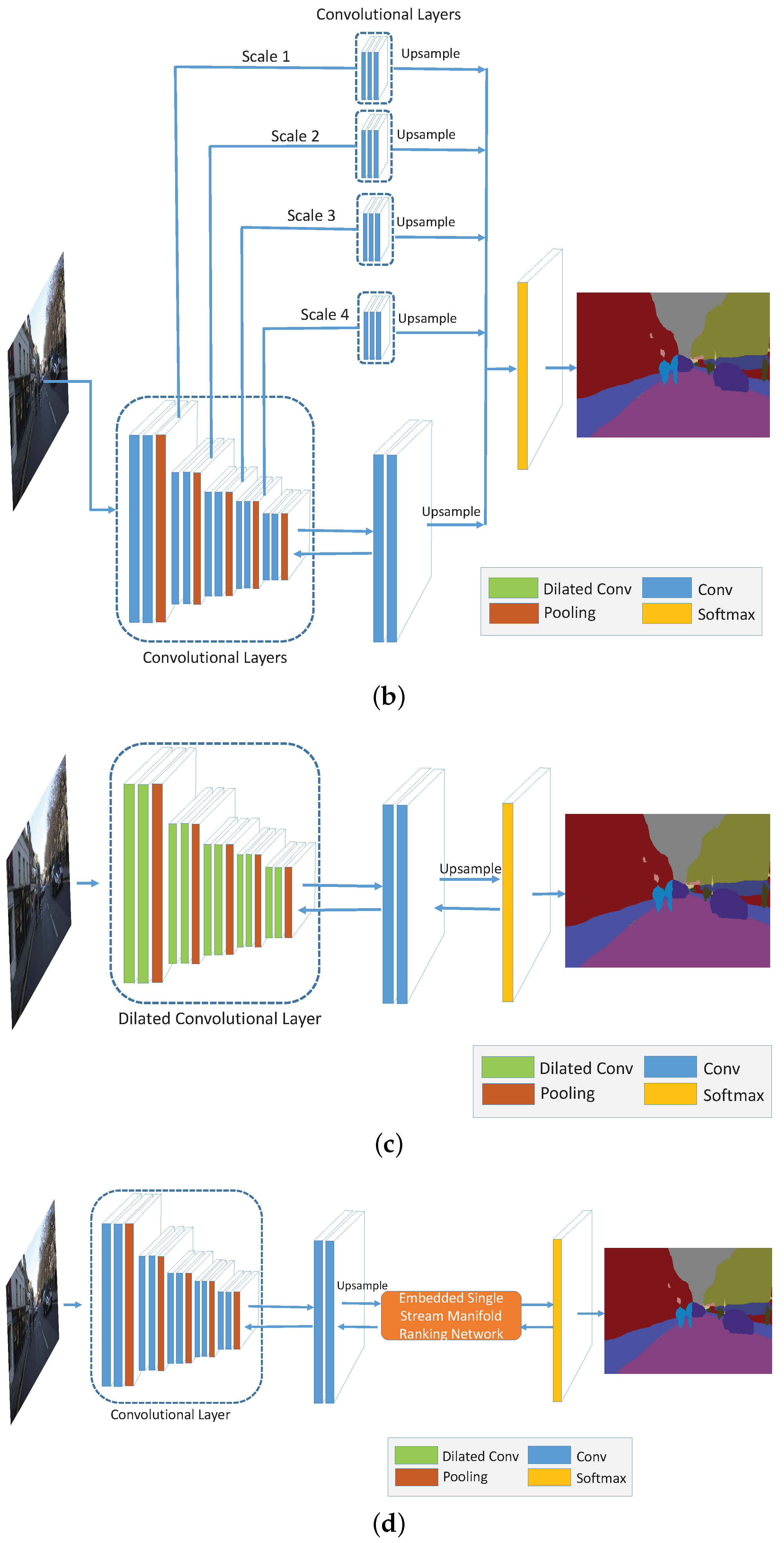
In this part, we explain in detail for the methods that employ only one of the three strategies, namely, multi-scale convolution (MS), broader receptive field (Dilated) and MR optimization (MR-opti) approaches. Figure A1 shows the general structures of these approaches and Table A1 presents the corresponding implementation parameters in each convolutional layer. In the table and figure, the “ReLU” active function [74] is implicitly employed in each convolutional layer. The network depicted in Figure A1a serves as the baseline convolutional network for comparison. Figure A1c,d are the networks that use only the dilated convolutional kernel [23] and manifold ranking optimization methods, respectively. The only difference between network in Figure A1a,c is the dilation kernel. In our experiment, we set the kernel sizes in each block as 6, 4, 2, 2 and 1, as illustrated in Table A1a. For the MR optimization layer embedded in the baseline network shown in Figure A1d, initial parameters of and are set to 3 and 5, respectively. Figure A1b presents the network with multi-scale strategy on the baseline network. After applying the pooling layer in each block, a convlutional block is adopted with three convolutional layers (named as poolx-conv-y in Table A1b. The scale is implicitly expressed in the pooling layer by factor 2.0.
Figure A1.
The architectures of the networks with different strategies: (a) Convolutional networks before employing the strategies (Before); (b) Networks using multi-scale strategy (MS); (c) Networks using dilated method (Dilated); (d) Networks using manifold ranking optimization (MR-Opti).
Figure A1.
The architectures of the networks with different strategies: (a) Convolutional networks before employing the strategies (Before); (b) Networks using multi-scale strategy (MS); (c) Networks using dilated method (Dilated); (d) Networks using manifold ranking optimization (MR-Opti).


Table A1.
Implementation details of the networks with different strategies.
| (a) Networks before Employing the Strategies (Before) | ||||||
| Block | Name | Kernel Size | Pad | Dilation | Stride | Number of Output |
| 0 | input | - | - | - | - | 3 |
| 1 | conv1-1 | 3 × 3 | 1 | 1 | 1 | 64 |
| conv1-2 | 3 × 3 | 1 | 1 | 1 | 64 | |
| pool1 | 3 × 3 | 1 | 0 | 1 | 64 | |
| 2 | conv2-1 | 3 × 3 | 1 | 1 | 1 | 128 |
| conv2-2 | 3 × 3 | 1 | 1 | 1 | 128 | |
| pool2 | 3 × 3 | 1 | 0 | 2 | 128 | |
| 3 | conv3-1 | 3 × 3 | 1 | 1 | 1 | 256 |
| conv3-2 | 3 × 3 | 1 | 1 | 1 | 256 | |
| pool3 | 3 × 3 | 1 | 0 | 2 | 256 | |
| 4 | conv4-1 | 3 × 3 | 1 | 1 | 1 | 512 |
| conv4-2 | 3 × 3 | 1 | 1 | 1 | 512 | |
| pool4 | 3 × 3 | 1 | 0 | 1 | 512 | |
| 5 | conv5-1 | 5 × 5 | 2 | 1 | 1 | 512 |
| conv5-2 | 5 × 5 | 2 | 1 | 1 | 512 | |
| pool5 | 3 × 3 | 1 | 0 | 1 | 512 | |
| - | fc6 | 3 × 3 | 1 | 1 | 1 | 1024 |
| fc7 | 1 × 1 | 0 | 1 | 1 | 1024 | |
| * | fc8 | 1 × 1 | 0 | 1 | 1 | 12 |
| - | output | 1 × 1 | 0 | 1 | 1 | 12 |
| (b) Networks Using Multi-Scale Strategy (MS) | ||||||
| Scale (Block) | Name | Kernel Size | Pad | Dilation | Stride | Number of Output |
| 0 | input | - | - | - | - | 3 |
| 1 | conv1-1 | 3 × 3 | 1 | 1 | 1 | 64 |
| conv1-2 | 3 × 3 | 1 | 1 | 1 | 64 | |
| pool1 | 3 × 3 | 1 | 0 | 2 | 64 | |
| 2 | conv2-1 | 3 × 3 | 1 | 1 | 1 | 128 |
| conv2-2 | 3 × 3 | 1 | 1 | 1 | 128 | |
| pool2 | 3 × 3 | 1 | 0 | 2 | 128 | |
| 3 | conv3-1 | 3 × 3 | 1 | 1 | 1 | 256 |
| conv3-2 | 3 × 3 | 1 | 1 | 1 | 256 | |
| pool3 | 3 × 3 | 1 | 0 | 2 | 256 | |
| 4 | conv4-1 | 3 × 3 | 1 | 1 | 1 | 512 |
| conv4-2 | 3 × 3 | 1 | 1 | 1 | 512 | |
| pool4 | 3 × 3 | 1 | 0 | 1 | 512 | |
| 5 | conv5-1 | 5 × 5 | 2 | 1 | 1 | 512 |
| conv5-2 | 5 × 5 | 2 | 1 | 1 | 512 | |
| pool5 | 3 × 3 | 1 | 0 | 1 | 512 | |
| - | fc6 | 3 × 3 | 1 | 1 | 1 | 1024 |
| fc7 | 1 × 1 | 0 | 1 | 1 | 1024 | |
| * | fc8 | 1 × 1 | 0 | 1 | 1 | 12 |
| 1 | pool1-conv-1 | 3 × 3 | 1 | 1 | 4 | 128 |
| pool1-conv-2 | 1 × 1 | 0 | 1 | 1 | 128 | |
| pool1-conv-3 | 1 × 1 | 0 | 1 | 1 | 12 | |
| 2 | pool2-conv-1 | 3 × 3 | 1 | 1 | 2 | 128 |
| pool2-conv-2 | 1 × 1 | 0 | 1 | 1 | 128 | |
| pool2-conv-3 | 1 × 1 | 0 | 1 | 1 | 12 | |
| 3 | pool3-conv-1 | 3 × 3 | 1 | 1 | 1 | 128 |
| pool3-conv-2 | 1 × 1 | 0 | 1 | 1 | 128 | |
| pool3-conv-3 | 1 × 1 | 0 | 1 | 1 | 12 | |
| 4 | pool4-conv-1 | 3 × 3 | 1 | 1 | 1 | 128 |
| pool4-conv-2 | 1 × 1 | 0 | 1 | 1 | 128 | |
| pool4-conv-3 | 1 × 1 | 0 | 1 | 1 | 12 | |
| - | output | 1 × 1 | 0 | 1 | 1 | 12 |
| (c) Networks Using Dilated Method (Dilated) | ||||||
| Block | Name | Kernel Size | Pad | Dilation | Stride | Number of Output |
| 0 | input | - | - | - | - | 3 |
| 1 | conv1-1 | 3 × 3 | 6 | 6 | 1 | 64 |
| conv1-2 | 3 × 3 | 6 | 6 | 1 | 64 | |
| pool1 | 3 × 3 | 1 | 0 | 2 | 64 | |
| 2 | conv2-1 | 3 × 3 | 4 | 4 | 1 | 128 |
| conv2-2 | 3 × 3 | 4 | 4 | 1 | 128 | |
| pool2 | 3 × 3 | 1 | 0 | 2 | 128 | |
| 3 | conv3-1 | 3 × 3 | 2 | 2 | 1 | 256 |
| conv3-2 | 3 × 3 | 2 | 2 | 1 | 256 | |
| pool3 | 3 × 3 | 1 | 0 | 2 | 256 | |
| 4 | conv4-1 | 3 × 3 | 2 | 2 | 1 | 512 |
| conv4-2 | 3 × 3 | 2 | 2 | 1 | 512 | |
| pool4 | 3 × 3 | 1 | 0 | 1 | 512 | |
| 5 | conv5-1 | 3 × 3 | 2 | 2 | 1 | 512 |
| conv5-2 | 3 × 3 | 2 | 2 | 1 | 512 | |
| pool5 | 3 × 3 | 1 | 0 | 1 | 512 | |
| - | fc6 | 3 × 3 | 1 | 1 | 1 | 1024 |
| fc7 | 1 × 1 | 0 | 1 | 1 | 1024 | |
| * | fc8 | 1 × 1 | 0 | 1 | 1 | 12 |
| - | output | 1 × 1 | 0 | 1 | 1 | 12 |
| (d) Networks Using Manifold Ranking Optimization (MR-Opti) | ||||||
| Block | Name | Kernel Size | Pad | Dilation | Stride | Number of Output |
| 0 | input | - | - | - | - | 3 |
| 1 | conv1-1 | 3 × 3 | 1 | 1 | 1 | 64 |
| conv1-2 | 3 × 3 | 1 | 1 | 1 | 64 | |
| pool1 | 3 × 3 | 1 | 0 | 1 | 64 | |
| 2 | conv2-1 | 3 × 3 | 1 | 1 | 1 | 128 |
| conv2-2 | 3 × 3 | 1 | 1 | 1 | 128 | |
| pool2 | 3 × 3 | 1 | 0 | 2 | 128 | |
| 3 | conv3-1 | 3 × 3 | 1 | 1 | 1 | 256 |
| conv3-2 | 3 × 3 | 1 | 1 | 1 | 256 | |
| pool3 | 3 × 3 | 1 | 0 | 2 | 256 | |
| 4 | conv4-1 | 3 × 3 | 1 | 1 | 1 | 512 |
| conv4-2 | 3 × 3 | 1 | 1 | 1 | 512 | |
| pool4 | 3 × 3 | 1 | 0 | 1 | 512 | |
| 5 | conv5-1 | 5 × 5 | 2 | 1 | 1 | 512 |
| conv5-2 | 5 × 5 | 2 | 1 | 1 | 512 | |
| pool5 | 3 × 3 | 1 | 0 | 1 | 512 | |
| - | fc6 | 3 × 3 | 1 | 1 | 1 | 1024 |
| fc7 | 1 × 1 | 0 | 1 | 1 | 1024 | |
| * | fc8 | 1 × 1 | 0 | 1 | 1 | 12 |
| - | Manifold Ranking Optimization | 12 | ||||
| - | output | 1 × 1 | 0 | 1 | 1 | 12 |
References
- Ladicky, L.; Torr, P.; Zisserman, A. Human Pose Estimation using a Joint Pixel-wise and Part-wise Formulation. In Proceedings of the 2013 IEEE Conference on Computer Vision and Pattern Recognition, Portland, OR, USA, 23–28 June 2013. [Google Scholar]
- Romera, E.; Bergasa, L.; Arroyo, R. Can we unify monocular detectors for autonomous driving by using the pixel-wise semantic segmentation of CNNs? arXiv, 2016; arXiv:1607.00971. [Google Scholar]
- Barrnes, D.; Maddern, W.; Posner, I. Find Your Own Way: Weakly-Supervised Segmentation of Path Proposals for Urban Autonomy. arXiv, 2016; arXiv:1610.01238. [Google Scholar]
- Kendall, A.; Cipolla, R. Modelling Uncertainty in Deep Learning for Camera Relocalization. arXiv, 2015; arXiv:1509.05909. [Google Scholar]
- Xiao, J.; Quan, L. Multiple View Semantic Segmentation for Street View Images. In Proceedings of the 2009 IEEE 12th International Conference on Computer Vision, Kyoto, Japan, 29 September–2 October 2009. [Google Scholar]
- Floros, G.; Leibe, B. Joint 2D-3D Temporally Consistent Semantic Segmentation of Street Scenes. In Proceedings of the 2012 IEEE Conference on Computer Vision and Pattern Recognition, Providence, RI, USA, 16–21 June 2012. [Google Scholar]
- Huval, B.; Wang, T.; Tandon, S.; Kiske, J.; Song, W.; Pazhayampallil, J.; Mujica, F. An empirical evaluation of deep learning on highway driving. arXiv, 2015; arXiv:1504.01716. [Google Scholar]
- Chen, C.; Seff, A.; Kornhauser, A.; Xiao, J. Deepdriving: Learning affordance for direct perception in autonomous driving. In Proceedings of the 2015 IEEE International Conference on Computer Vision, Santiago, Chile, 7–13 December 2015. [Google Scholar]
- Toshev, A.; Szegedy, C. DeepPose: Human Pose Estimation via Deep Neural Networks. arXiv, 2014; arXiv:1312.4659. [Google Scholar]
- Tompson, J.J.; Jain, A.; LeCun, Y.; Bregler, C. Joint training of a convolutional network and a graphical model for human pose estimation. arXiv, 2014; arXiv:1406.2984. [Google Scholar]
- Jackson, A.; Valstar, M.; Tzimiropoulos, G. A CNN Cascade for Landmark Guided Semantic Part Segmentation. arXiv, 2016; arXiv:1609.09642. [Google Scholar]
- Maggiori, E.; Tarabalka, Y.; Charpiat, G.; Alliez, P. High-Resolution Semantic Labeling with Convolutional Neural Networks. arXiv, 2016; arXiv:1611.01962. [Google Scholar]
- Kampffmeyer, M.; Salberg, A.B.; Jenssen, R. Semantic segmentation of small objects and modeling of uncertainty in urban remote sensing images using deep convolutional neural networks. In Proceedings of the 2016 IEEE Conference on Computer Vision and Pattern Recognition Workshops (CVPRW), Las Vegas, NV, USA, 26 June–1 July 2016. [Google Scholar]
- Audebert, N.; Saux, B.L.; Lefèvre, S. Semantic Segmentation of Earth Observation Data Using Multimodal and Multi-scale Deep Networks. arXiv, 2016; arXiv:1609.06846. [Google Scholar]
- Längkvist, M.; Kiselev, A.; Alirezaie, M.; Loutfi, A. Classification and segmentation of satellite orthoimagery using convolutional neural networks. Remote Sens. 2016, 8, 329. [Google Scholar] [CrossRef]
- Muruganandham, S. Semantic Segmentation of Satellite Images Using Deep Learning. Master’s Thesis, Department of Computer Science, Electrical and Space Engineering, Luleå University of Technology, Luleå, Sweden, 2016. [Google Scholar]
- Wu, Z.; Song, S.; Khosla, A.; Yu, F.; Zhang, L.; Tang, X.; Xiao, J. 3d Shapenets: A Deep Representation for Volumetric Shapes; Princeton University: Princeton, NJ, USA, 2015. [Google Scholar]
- Kendall, A.; Grimes, M.; Cipolla, R. PoseNet: A Convolutional Network for Real-Time 6-DOF Camera Relocalization. arXiv, 2016; arXiv:1505.07427. [Google Scholar]
- Barron, J.T.; Poole, B. The fast bilateral solver. arXiv, 2016; arXiv:1511.03296. [Google Scholar]
- Mostajabi, M.; Yadollahpour, P.; Shakhnarovich, G. Feedforward semantic segmentation with zoom-out features. arXiv, 2015; arXiv:1412.0774v1. [Google Scholar]
- Dai, J.; He, K.; Sun, J. Instance-aware Semantic Segmentation via Multi-task Network Cascades. arXiv, 2015; arXiv:1512.04412. [Google Scholar]
- Shelhamer, E.; Long, J.; Darrell, T. Fully Convolutional Networks for Semantic Segmentation. arXiv, 2015; arXiv:1605.06211. [Google Scholar]
- Yu, F.; Koltun, V. Multi-Scale Context Aggregation by Dilated Convolutions. arXiv, 2016; arXiv:1511.07122. [Google Scholar]
- Chen, L.; Papandreou, G.; Kokkinos, I.; Murphy, K.; Yuille, A. DeepLab: Semantic Image Segmentation with Deep Convolutional Nets, Atrous Convolution, and Fully Connected CRFs. arXiv, 2015; arXiv:1606.00915. [Google Scholar]
- Zheng, S.; Jayasumana, S.; Paredes, B.; Vineet, V.; Su, Z.; Du, D.; Huang, C.; Torr, P. Conditional Random Fields as Recurrent Neural Networks. arXiv, 2015; arXiv:1502.03240. [Google Scholar]
- Chandra, S.; Kokkinos, I. Fast, Exact and Multi-Scale Inference for Semantic Image Segmentation with Deep Gaussian CRFs. arXiv, 2016; arXiv:1603.08358. [Google Scholar]
- Badrinarayanan, V.; Handa, A.; Cipolla, R. SegNet: A Deep Convolutional Encoder-Decoder Architecture for Image Segmentation. arXiv, 2015; arXiv:1511.00561. [Google Scholar]
- Hyeonwoo, N.; Hong, S.; Han, B. Learning deconvolution network for semantic segmentation. arXiv, 2015; arXiv:1505.04366. [Google Scholar]
- Lin, G.; Shen, C.; Hengel, A.; Reid, I. Efficient piecewise training of deep structured models for semantic segmentation. arXiv, 2016; arXiv:1504.01013. [Google Scholar]
- Eigen, D.; Fergus, R. Predicting Depth, Surface Normals and Semantic Labels with a Common Multi-Scale Convolutional Architecture. arXiv, 2015; arXiv:1411.4734. [Google Scholar]
- Chen, L.; Schwing, A.; Yuille, A.; Urtasun, R. Learning Deep Structured Models. arXiv, 2015; arXiv:1407.2538. [Google Scholar]
- Chen, L.; Papandreou, G.; Kokkinos, I.; Murphy, K.; Yuille, A. Semantic Image Segmentation with Deep Convolutional Nets and Fully Connected CRFs. arXiv, 2015; arXiv:1412.7062. [Google Scholar]
- Krähenbühl, P.; Koltun, V. Efficient Inference in Fully Connected CRFs with Gaussian Edge Potentials. arXiv, 2012; arXiv:1210.5644. [Google Scholar]
- Arnab, A.; Jayasumana, S.; Zheng, S.; Torr, P. Higher Order Conditional Random Fields in Deep Neural Networks. arXiv, 2016; arXiv:1511.08119. [Google Scholar]
- Vemulapalli, R.; Tuzel, O.; Liu, M.; Chellappa, R. Gaussian Conditional Random Field Network for Semantic Segmentation. In Proceedings of the 2016 IEEE Conference on Computer Vision and Pattern Recognition (CVPR), Las Vegas, NV, USA, 27–30 June 2016. [Google Scholar]
- Zhou, D.; Weston, J.; Gretton, A.; Bousquent, O.; Scholkopf, B. Ranking on data manifolds. In Proceedings of the 16th International Conference on Neural Information Processing Systems, Whistler, BC, Canada, 9–11 December 2003. [Google Scholar]
- Zhou, D.; Bousquent, O.; Lal, T.; Weston, J.; Scholkopf, B. Learning with Local and Global Consistency. In Proceedings of the 16th International Conference on Neural Information Processing Systems, Whistler, BC, Canada, 9–11 December 2003. [Google Scholar]
- Yang, C.; Zhang, L.; Lu, H.; Ruan, X.; Yang, M. Saliency Detection via Graph-Based Manifold Ranking. In Proceedings of the 2013 IEEE Conference on Computer Vision and Pattern Recognition, Portland, OR, USA, 23–28 June 2013. [Google Scholar]
- Bencherif, M.A.; Bazi, Y.; Guessoum, A.; Alajlan, N.; Melgani, F.; AlHichri, H. Fusion of Extreme Learning Machine and Graph-Based Optimization Methods for Active Classification of Remote Sensing Images. IEEE Geosci. Remote Sens. Lett. 2015, 12, 527–531. [Google Scholar] [CrossRef]
- Krähenbühl, P.; Koltun, V. Parameter Learning and Convergent Inference for Dense Random Fields. In Proceedings of the 30th International Conference on Machine Learning, Atlanta, GA, USA, 16–21 June 2013. [Google Scholar]
- Gupta, S.; Girshick, R.; Arbeláez, P.; Malik, J. Learning Rich Features from RGB-D Images for Object Detection and Segmentation. arXiv, 2014; arXiv:1407.5736. [Google Scholar]
- Hariharan, B.; Arbeláez, P.; Girshick, R.; Malik, J. Simultaneous Detection and Segmentation. arXiv, 2014; arXiv:1407.1808. [Google Scholar]
- Dai, J.; He, K.; Sun, J. Convolutional Feature Masking for Joint Object and Stuff Segmentation. arXiv, 2015; arXiv:1412.1283. [Google Scholar]
- Farabet, C.; Couprie, C.; Najman, L.; LeCun, Y. Learning Hierarchical Features for Scene Labeling. IEEE Trans. Pattern Anal. Mach. Intell. 2013, 35, 1915–1929. [Google Scholar] [CrossRef] [PubMed]
- Chen, L.; Yang, Y.; Wang, J.; Xu, W.; Yuille, A. Attention to Scale: Scale-aware Semantic Image Segmentation. arXiv, 2016; arXiv:1511.03339. [Google Scholar]
- Bearman, A.; Russakovsky, O.; Ferrari, V.; Li, F.F. What’s the Point: Semantic Segmentation with Point Supervision. arXiv, 2016; arXiv:1506.02106. [Google Scholar]
- Romero, A.; Gatta, C.; Camps-Valls, G. Unsupervised Deep Feature Extraction for Remote Sensing Image Classification. IEEE Trans. Geosci. Remote Sens. 2015, 54, 1349–1362. [Google Scholar] [CrossRef]
- Campos-Taberner, M.; Romero-Soriano, A.; Gatta, C.; Camps-Valls, G.; Lagrange, A.; Le Saux, B.; Randrianarivo, H. Processing of Extremely High-Resolution LiDAR and RGB Data: Outcome of the 2015 IEEE GRSS Data Fusion Contest–Part A: 2-D Contest. IEEE J. Sel. Top. Appl. Earth Obs. Remote Sens. 2016, 9, 5547–5559. [Google Scholar] [CrossRef]
- Tschannen, M.; Cavigelli, L.; Mentzer, F.; Wiatowski, T.; Benini, L. Deep Structured Features for Semantic Segmentation. arXiv, 2016; arXiv:1609.07916. [Google Scholar]
- Piramanayagam, S.; Schwartzkopf, W.; Koehler, F.W.; Saber, E. Classification of remote sensed images using random forests and deep learning framework. SPIE Remote Sens. Int. Soc. Opt. Photonics 2016. [Google Scholar] [CrossRef]
- Marcu, A.; Leordeanu, M. Dual Local-Global Contextual Pathways for Recognition in Aerial Imagery. arXiv, 2016; arXiv:1605.05462. [Google Scholar]
- Yuan, Y.; Lin, J.; Wang, Q. Dual-clustering-based hyperspectral band selection by contextual analysis. IEEE Trans. Geosci. Remote Sens. 2016, 54, 1431–1445. [Google Scholar] [CrossRef]
- Kendall, A.; Badrinarayanan, V.; Cipolla, R. Bayesian SegNet: Model Uncertainty in Deep Convolutional Encoder-Decoder Architectures for Scene Understanding. arXiv, 2015; arXiv:1511.02680. [Google Scholar]
- Simonyan, K.; Zisserman, A. Very Deep Convolutional Networks for Large-Scale Image Recognition. arXiv, 2015; arXiv:1409.1556. [Google Scholar]
- Hong, S.; Noh, H.; Han, B. Decoupled Deep Neural Network for Semi-supervised Semantic Segmentation. arXiv, 2015; arXiv:1506.04924. [Google Scholar]
- Audebert, N.; Saux, B.L.; Lefèvre, S. Segment-before-Detect: Vehicle Detection and Classification through Semantic Segmentation of Aerial Images. Remote Sens. 2017, 9, 368. [Google Scholar] [CrossRef]
- Huang, Z.; Cheng, G.; Wang, H.; Li, H.; Shi, L.; Pan, C. Building extraction from multi-source remote sensing images via deep deconvolution neural networks. In Proceedings of the IEEE International Geoscience and Remote Sensing Symposium (IGARSS), Beijing, China, 10–15 July 2016. [Google Scholar]
- Audebert, N.; Boulch, A.; Lagrange, A.; Le Saux, B.; Lefevre, S. Deep Learning for Remote Sensing; Technical Report; ONERA The French Aerospace Lab, DTIM & Univ. Bretagne-Sud & ENSTA ParisTech: Palaiseau, France, 2016. [Google Scholar]
- Paisitkriangkrai, S.; Sherrah, J.; Janney, P.; Hengel, V.D. Effective semantic pixel labelling with convolutional networks and conditional random fields. In Proceedings of the 2015 IEEE Conference on Computer Vision and Pattern Recognition Workshops, Boston, MA, USA, 7–12 June 2015. [Google Scholar]
- Alam, F.I.; Zhou, J.; Liew, A.W.C.; Jia, X. CRF learning with CNN features for hyperspectral image segmentation. In Proceedings of the IEEE International Geoscience and Remote Sensing Symposium, Beijing, China, 10–15 July 2016. [Google Scholar]
- He, X.; Cai, D.; Niyogi, P. Laplacian Score for Feature Selection. In Proceedings of the 18th International Conference on Neural Information Processing Systems, Vancouver, BC, Canada, 5–8 December 2005. [Google Scholar]
- Quan, R.; Han, J.; Zhang, D.; Nie, F. Object co-segmentation via graph optimized-flexible manifold ranking. In Proceedings of the 2016 IEEE Conference on Computer Vision and Pattern Recognition (CVPR), Las Vegas, NV, USA, 27–30 June 2016. [Google Scholar]
- Wang, Q.; Lin, J.; Yuan, Y. Salient band selection for hyperspectral image classification via manifold ranking. IEEE Trans. Neural Netw. Learn. Syst. 2016, 27, 1279–1289. [Google Scholar] [CrossRef] [PubMed]
- Yang, C.; Zhang, L.; Lu, H. Graph-regularized saliency detection with convex-hull-based center prior. IEEE Signal Process. Lett. 2013, 20, 637–640. [Google Scholar] [CrossRef]
- Xu, B.; Bu, J.; Chen, C.; Cai, D.; He, X.; Liu, W.; Luo, J. Efficient Manifold Ranking for Image Retrieval. In Proceedings of the 34th international ACM SIGIR Conference on Research and Development in Information Retrieval, Beijing, China, 24–28 July 2011. [Google Scholar]
- Hsieh, C.; Han, C.; Shih, J.; Lee, C.; Fan, K. 3D Model Retrieval Using Multiple Features and Manifold Ranking. In Proceedings of the 2015 8th International Conference on Ubi-Media Computing (UMEDIA), Colombo, Sri Lanka, 24–26 August 2015. [Google Scholar]
- Zhou, T.; He, X.; Xie, K.; Fu, K.; Zhang, J.; Yang, J. Robust visual tracking via efficient manifold ranking with low-dimensional compressive features. Pattern Recognit. 2015, 48, 2459–2473. [Google Scholar] [CrossRef]
- Brostow, G.; Shotton, J.; Fauqueur, J.; Cipolla, R. Segmentation and Recognition Using Structure from Motion Point Clouds. In Proceedings of the 10th European Conference on Computer Vision, Marseille, France, 12–18 October 2008. [Google Scholar]
- Brostow, G.; Fauqueur, J.; Cipolla, R. Semantic object classes in video: A high-definition ground truth database. Pattern Recognit. Lett. 2009, 30, 88–97. [Google Scholar] [CrossRef]
- Ruder, S. An overview of gradient descent optimization algorithms. arXiv, 2016; arXiv:1609.04747. [Google Scholar]
- He, K.; Zhang, X.; Ren, S.; Sun, J. Deep Residual Learning for Image Recognition. arXiv, 2015; arXiv:1512.03385. [Google Scholar]
- Everingham, M.; Gool, L.; Williams, C.K.I.; Winn, J.; Zisserman, A. The Pascal Visual Object Classes (VOC) Challenge. Int. J. Comput. Vis. 2010, 88, 303–338. [Google Scholar] [CrossRef]
- Rottensteiner, F.; Sohn, G.; Jung, J.; Gerke, M.; Baillard, C.; Benitez, S.; Breitkopf, U. The ISPRS benchmark on urban object classification and 3D building reconstruction. ISPRS Ann. Photogramm. Remote Sens. Spat. Inf. Sci. 2012, I-3, 293–298. [Google Scholar] [CrossRef]
- Glorot, X.; Bordes, A.; Bengio, Y. Deep Sparse Rectifier Neural Networks. In Proceedings of the 14th International Conference on Artificial Intelligence and Statistics, Fort Lauderdale, FL, USA, 11–13 April 2011; Volume 15, pp. 315–323. [Google Scholar]
- Jia, Y.; Shelhamer, E.; Donahue, J.; Karayev, S.; Long, J.; Girshick, R.; Guadarrama, S.; Darrell, T. Caffe: Convolutional Architecture for Fast Feature Embedding. In Proceedings of the 22nd ACM International Conference on Multimedia, Orlando, FL, USA, 3–7 November 2014. [Google Scholar]
- Marmanis, D.; Wegner, J.D.; Galliani, S.; Schindler, K.; Datcu, M.; Stilla, U. Semantic Segmentation of Aerial Images with an Ensemble of CNSS. ISPRS Ann. Photogramm. Remote Sens. Spat. Inf. Sci. 2016, 3, 473–480. [Google Scholar] [CrossRef]
- Hariharan, B.; Arbeláez, P.; Bourdev, L.; Maji, S.; Malik, J. Semantic Contours from Inverse Detectors. In Proceedings of the 2011 IEEE International Conference on Computer Vision (ICCV), Barcelona, Spain, 6–13 November 2011. [Google Scholar]
- Zoran, D.; Weiss, Y. From Learning Models of Natural Image Patches to Whole Image Restoration. In Proceedings of the 2011 IEEE International Conference on Computer Vision (ICCV), Barcelona, Spain, 6–13 November 2011. [Google Scholar]
- Lin, T.; Maire, M.; Belongie, S.; Bourdev, L.; Girshick, R.; Hays, J.; Perona, P.; Ramanan, D.; Zitnick, C.; Dollár, P. Microsoft coco: Common objects in context. arXiv, 2014; arXiv:1405.0312. [Google Scholar]
- Lin, G.; Milan, A.; Shen, C.; Reid, I. RefineNet: Multi-Path Refinement Networks with Identity Mappings for High-Resolution Semantic Segmentation. arXiv, 2016; arXiv:1611.06612. [Google Scholar]
- Kohli, P.; Torr, P.H. Robust higher order potentials for enforcing label consistency. Int. J. Comput. Vis. 2009, 82, 302–324. [Google Scholar] [CrossRef]
- Krizhevsky, A.; Sutskever, I.; Hinton, G.E. Imagenet classification with deep convolutional neural networks. In Proceedings of the 25th International Conference on Neural Information Processing Systems, Lake Tahoe, NV, USA, 3–6 December 2012. [Google Scholar]
- Quang, N.T.; Thuy, N.T.; Sang, D.V.; Binh, H.T.T. An efficient framework for pixel-wise building segmentation from aerial images. In Proceedings of the Sixth International Symposium on Information and Communication Technology, Hue City, Vietnam, 3–4 December 2015. [Google Scholar]
- Boulch, A. DAG of Convolutional Networks for Semantic Labeling; Technical Report; Office National d’études et de Recherches Aérospatiales: Palaiseau, France, 2015. [Google Scholar]
- Gerke, M.; Speldekamp, T.; Fries, C.; Gevaert, C. Automatic semantic labelling of urban areas using a rule-based approach and realized with mevislab. Unpublished 2015. [Google Scholar] [CrossRef]
- Sherrah, J. Fully convolutional networks for dense semantic labelling of high-resolution aerial imagery. arXiv, 2016; arXiv:1606.02585. [Google Scholar]
- Gerke, M. Use of the Stair Vision Library within the ISPRS 2D Semantic Labeling Benchmark (Vaihingen); Technical Report; University of Twente: Enschede, The Netherlands, 2015. [Google Scholar]
- Petersen, K.; Pedersen, M. The Matrix Cookbook; Technical University of Denmark: Kongens Lyngby, Denmark, 2008. [Google Scholar]
- The National Survey of Geographical Conditions Leading Group Office, Sate Council, P.R.C. General Situation and Index of Geographical Conditions (Chinese Manual, GDPJ 01-2013); The National Survey of Geographical Conditions Leading Group Office, Sate Council, P.R.C.: Beijing, China, 2013. [Google Scholar]
- Immitzer, M.; Atzberger, C.; Koukal, T. Tree species classification with random forest using very high spatial resolution 8-band WorldView-2 satellite data. Remote Sens. 2012, 4, 2661–2693. [Google Scholar] [CrossRef]
- Dribault, Y.; Chokmani, K.; Bernier, M. Monitoring seasonal hydrological dynamics of minerotrophic peatlands using multi-date GeoEye-1 very high resolution imagery and object-based classification. Remote Sens. 2012, 4, 1887–1912. [Google Scholar] [CrossRef]
- Onojeghuo, A.O.; Blackburn, G.A. Mapping reedbed habitats using texture-based classification of QuickBird imagery. Int. J. Remote Sens. 2011, 32, 8121–8138. [Google Scholar] [CrossRef]
- Junwei, S.; Youjing, Z.; Xinchuan, L.; Wenzhi, Y. Comparison between GF-1 and Landsat-8 images in land cover classification. Prog. Geogr. 2016, 35, 255–263. [Google Scholar]
- Goodfellow, I.; Pouget-Abadie, J.; Mirza, M.; Xu, B.; Warde-Farley, D.; Ozair, S.; Courville, A.; Bengio, Y. Generative adversarial nets. In Advances in Neural Information Processing Systems; The MIT Press: Cambridge, MA, USA, 2014; pp. 2672–2680. [Google Scholar]
- Mirza, M.; Osindero, S. Conditional generative adversarial nets. arXiv, 2014; arXiv:1411.1784. [Google Scholar]
- Luc, P.; Couprie, C.; Chintala, S.; Verbeek, J. Semantic Segmentation using Adversarial Networks. arXiv, 2016; arXiv:1611.08408. [Google Scholar]
Figure 1.
Dual multi-scale manifold ranking (DMSMR) network overview. For each dilated convolutional layer, a non-dilated convolution layer is applied following the pooling layer in each scale. The dilated and non-dilated convolution layers form a dual layer, in which the corresponding layers are optimized with the embedded feedforward single stream manifold ranking network. The scale factor is implicitly represented by the pooling layer in each block. Figure 2 illustrates how to embed the manifold ranking optimization method into the single stream network (marked with orange color in this figure). The optimized outputs of each scale, that is, generated in each scale, are combined by Equation (17).

Figure 2.
The embedded feedforward single stream manifold ranking optimization network. The output of the convolutional features that upsample to full image resolution for each class, such as road, sky and building, within the CamVid dataset [68,69] depicted in the figure, serves as the initial manifold ranking score to be optimized. By applying the feedforward MR inference with the contextual information extracted from the input image, the optimal MR score of each class can be obtained by Equation (10). The only requirement for the proposed network is the multi-label neighborhood relationship, which is designed for constructing the Laplacian matrix in a single stream rather than the unary and pairwise streams presented in [26,29].

Figure 3.
Several semantic segmentation results on PASCAL VOC 2012 validation images. DMSMR: Semantic segmentation result predicted by dual multi-scale manifold ranking network. GT: Ground Truth.
Figure 3.
Several semantic segmentation results on PASCAL VOC 2012 validation images. DMSMR: Semantic segmentation result predicted by dual multi-scale manifold ranking network. GT: Ground Truth.

Figure 4.
Semantic segmentation results on CamVid images. DMSMR: Semantic segmentation result predicted by dual multi-scale manifold ranking network (DMSMR). GT: Ground Truth.
Figure 4.
Semantic segmentation results on CamVid images. DMSMR: Semantic segmentation result predicted by dual multi-scale manifold ranking network (DMSMR). GT: Ground Truth.

Figure 5.
Accuracy analysis with respect to boundary on CamVid dataset. (a) Trimap visualization on CamVid dataset. Top-left: source image. Top-right: ground truth. Bottom-left: trimap with one pixel band width. Bottom-right: trimap with three pixels band width. (b) Pixel mIoU with respect to band width around object boundaries. We measure the relationship of our model before and after employing the multi-scale (MS), dilated convolution (Dilated), single stream Manifold Ranking (MR-Opti) and joint strategies (DMSMR).

Figure 6.
Visualization of the comparative results on a few Vaihingen testing imagery (tile numbers 2, 4, 6 and 8). For each image, we generate the dense prediction results and corresponding error maps (red/green image) with different approaches.
Figure 6.
Visualization of the comparative results on a few Vaihingen testing imagery (tile numbers 2, 4, 6 and 8). For each image, we generate the dense prediction results and corresponding error maps (red/green image) with different approaches.

Figure 7.
Semantic segmentation results with different strategies on the EvLab-SS validation patches. Four kinds of image patches with different spatial resolutions and illuminations are depicted in the figure. The first and second rows are the GeoEye and World-View 2 satellite images with resample GSD of 0.5 m and 0.2 m. The third and the last rows are the aerial images with resample GSD of 0.25 m and 0.1 m, respectively. MS: Predictions with multi-scale approach. MR-Opti: Semantic segmentation results using manifold ranking optimization method. DMSMR: Segmentation result predicted by dual multi-scale manifold ranking network. GT: Ground Truth.

Figure 8.
Accuracy analysis with respect to boundary on EvLab-SS dataset. (a) Visualization of trimap for EvLab-SS dataset. Top-left: source patch. Top-right: ground truth. Bottom-left: trimap with one pixel band width. Bottom-right: trimap with three pixels band width. (b) Pixel mIoU with respect to band width around object boundaries. We measure the relationship for our model before and after employing the multi-scale (MS), dilated convolution (Dilated), single stream Manifold Ranking (MR-Opti) and joint strategies (DMSMR) on the EvLab-SS dataset.

Table 1.
Detailed implementation of the DMSMR networks.
| (a) Dilated Convolutional Layers | ||||||
|---|---|---|---|---|---|---|
| Scale (Block) | Name | Kernel Size | Pad | Dilation | Stride | Number of Output |
| 0 | input | - | - | - | - | 3 |
| 1 | conv1-1 | 3 × 3 | 6 | 6 | 1 | 64 |
| conv1-2 | 3 × 3 | 6 | 6 | 1 | 64 | |
| pool1 | 3 × 3 | 1 | 0 | 2 | 64 | |
| 2 | conv2-1 | 3 × 3 | 4 | 4 | 1 | 128 |
| conv2-2 | 3 × 3 | 4 | 4 | 1 | 128 | |
| pool2 | 3 × 3 | 1 | 0 | 2 | 128 | |
| 3 | conv3-1 | 3 × 3 | 2 | 2 | 1 | 256 |
| conv3-2 | 3 × 3 | 2 | 2 | 1 | 256 | |
| pool3 | 3 × 3 | 1 | 0 | 2 | 256 | |
| 4 | conv4-1 | 3 × 3 | 2 | 2 | 1 | 512 |
| conv4-2 | 3 × 3 | 2 | 2 | 1 | 512 | |
| pool4 | 3 × 3 | 1 | 0 | 1 | 512 | |
| 5 | conv5-1 | 3 × 3 | 2 | 2 | 1 | 512 |
| conv5-2 | 3 × 3 | 2 | 2 | 1 | 512 | |
| pool5 | 3 × 3 | 1 | 0 | 1 | 512 | |
| - | fc6 | 3 × 3 | 1 | 1 | 1 | 1024 |
| fc7 | 1 × 1 | 0 | 1 | 1 | 1024 | |
| * | fc8 | 1 × 1 | 0 | 1 | 1 | 12 |
| - | Manifold Ranking Optimization | 12 | ||||
| (b) Non-Dilated Convolutional Layers | ||||||
| Scale (Block) | Name | Kernel Size | Pad | Dilation | Stride | Output Size |
| 1 | pool1-conv-1 | 3 × 3 | 1 | 1 | 4 | 128 |
| pool1-conv-2 | 1 × 1 | 0 | 1 | 1 | 128 | |
| pool1-conv-3 | 1 × 1 | 0 | 1 | 1 | 12 | |
| - | Manifold Ranking Optimization | 12 | ||||
| 2 | pool2-conv-1 | 3 × 3 | 1 | 1 | 2 | 128 |
| pool2-conv-2 | 1 × 1 | 0 | 1 | 1 | 128 | |
| pool2-conv-3 | 1 × 1 | 0 | 1 | 1 | 12 | |
| - | Manifold Ranking Optimization | 12 | ||||
| 3 | pool3-conv-1 | 3 × 3 | 1 | 1 | 1 | 128 |
| pool3-conv-2 | 1 × 1 | 0 | 1 | 1 | 128 | |
| pool3-conv-3 | 1 × 1 | 0 | 1 | 1 | 12 | |
| - | Manifold Ranking Optimization | 12 | ||||
| 4 | pool4-conv-1 | 3 × 3 | 1 | 1 | 1 | 128 |
| pool4-conv-2 | 1 × 1 | 0 | 1 | 1 | 128 | |
| pool4-conv-3 | 1 × 1 | 0 | 1 | 1 | 12 | |
| - | Manifold Ranking Optimization | 12 | ||||
Table 2.
PASCAL VOC12 dataset [72] results. We compare our proposed network with recent methods that support inference techniques. Additional aides, such as region proposal, multi-stage inference, and extra unary initialized model, are unnecessary in our approach. Some of the methods use the CRF as a post optimization procedure. In contrast, our proposed approach achieves competitive accuracy without post-processing in an end-to-end manner.
| Aeroplane | Bicycle | Bird | Boat | Bottle | Bus | Car | Cat | Chair | Cow | Diningtable | Dog | Horse | Motorbike | Person | Pottedplant | Sheep | Sofa | Train | Tvmonitor | Mean IoU | |
|---|---|---|---|---|---|---|---|---|---|---|---|---|---|---|---|---|---|---|---|---|---|
| SegNet [27] | 73.6 | 37.6 | 62.0 | 46.8 | 58.6 | 79.1 | 70.1 | 65.4 | 23.6 | 60.4 | 45.6 | 61.8 | 63.5 | 75.3 | 74.9 | 42.6 | 63.7 | 42.5 | 67.8 | 52.7 | 59.9 |
| FCN-8s [22] (Multi-stage training) | 76.8 | 34.2 | 68.9 | 49.4 | 60.3 | 75.3 | 74.7 | 77.6 | 21.4 | 62.5 | 46.8 | 71.8 | 63.9 | 76.5 | 73.9 | 45.2 | 72.4 | 37.4 | 70.9 | 55.1 | 62.2 |
| DeepLab-Msc [24] (VGG-16 initialization) | 74.9 | 34.1 | 72.6 | 52.9 | 61.0 | 77.9 | 73.0 | 73.7 | 26.4 | 62.2 | 49.3 | 68.4 | 64.1 | 74.0 | 75.0 | 51.7 | 72.7 | 42.5 | 67.2 | 55.7 | 62.9 |
| DilatedConv Front end [28] (VGG-16 initialization) | 82.2 | 37.4 | 72.7 | 57.1 | 62.7 | 82.8 | 77.8 | 78.9 | 28 | 70 | 51.6 | 73.1 | 72.8 | 81.5 | 79.1 | 56.6 | 77.1 | 49.9 | 75.3 | 60.9 | 67.6 |
| DeconvNet + CRF [28] (Region Proposals) | 87.8 | 41.9 | 80.6 | 63.9 | 67.3 | 88.1 | 78.4 | 81.3 | 25.9 | 73.7 | 61.2 | 72.0 | 77.0 | 79.9 | 78.7 | 59.5 | 78.3 | 55.0 | 75.2 | 61.5 | 70.5 |
| CRF-RNN [25] (Multi-stage training) | 87.5 | 39.0 | 79.7 | 64.2 | 68.3 | 87.6 | 80.8 | 84.4 | 30.4 | 78.2 | 60.4 | 80.5 | 77.8 | 83.1 | 80.6 | 59.5 | 82.8 | 47.8 | 78.3 | 67.1 | 72.0 |
| DMSMR | 87.6 | 40.3 | 80.6 | 62.9 | 71.3 | 88.1 | 84.4 | 84.7 | 29.6 | 77.8 | 58.5 | 79.9 | 80.9 | 85.4 | 82.1 | 54.9 | 83.8 | 48.2 | 80.2 | 65.3 | 72.4 |
| G-CRF [35] (Unary Initialized with DeepLab CNN) | 85.2 | 43.9 | 83.3 | 65.2 | 68.3 | 89.0 | 82.7 | 85.3 | 31.1 | 79.5 | 63.3 | 80.5 | 79.3 | 85.5 | 81.0 | 60.5 | 85.5 | 52.0 | 77.3 | 65.1 | 73.2 |
Table 3.
Quantitative evaluation of the semantic segmentation results on CamVid dataset [68,69]. The proposed DMSMR approach outperforms the methods employing only one strategy.
| Building | Tree | Sky | Car | Sign | Road | Pedestrian | Fence | Pole | Sidewalk | Bicyclist | Mean IoU | |
|---|---|---|---|---|---|---|---|---|---|---|---|---|
| Before | 45.5 | 73.5 | 78.0 | 23.7 | 14.5 | 87.2 | 11.3 | 36.9 | 2.5 | 74.3 | 13.1 | 41.9 |
| MS | 81.4 | 88.1 | 80.3 | 40.1 | 16.3 | 95.6 | 26.2 | 40.0 | 3.7 | 82.0 | 37.4 | 53.7 |
| Dilated | 59.8 | 82.8 | 79.5 | 29.0 | 19.4 | 91.0 | 17.5 | 48.0 | 6.7 | 81.2 | 44.7 | 50.9 |
| MR-Opti | 90.6 | 95.1 | 74.6 | 94.6 | 21.9 | 98.2 | 53.1 | 64.3 | 9.8 | 92.6 | 42.1 | 54.8 |
| DMSMR | 93.1 | 94.5 | 82.9 | 92.7 | 45.5 | 97.4 | 72.5 | 77.2 | 7.2 | 94.5 | 68.9 | 63.6 |
Table 4.
Vaihingen dataset [88] results. We compare our proposed approach with a few recent state-of-the-art methods listed on the ISPRS Vaihingen 2D contest leader board. Traditional approaches and methods that employ additional aides (methods with qualifying comments) are referenced for comparison.
| Imp.surf. | Building | Low veg. | Tree | Car | Overall F1 | Overall Acc. | |
|---|---|---|---|---|---|---|---|
| SVL [87] (Feature based) | 86.1 | 90.9 | 77.6 | 84.9 | 59.9 | 79.88 | 84.7 |
| ADL [59] (CRF post-processing) | 89.0 | 93.0 | 81.0 | 87.8 | 59.5 | 82.06 | 87.3 |
| UT_Mev [85] (DSM supported) | 84.3 | 88.7 | 74.5 | 82.0 | 9.9 | 67.88 | 81.8 |
| HUST [83] (CRF post-processing) | 86.9 | 92.0 | 78.3 | 86.9 | 29.0 | 74.62 | 85.9 |
| ONE [84] (VGG-16 pre-trained model) | 87.8 | 92.0 | 77.8 | 86.2 | 50.7 | 78.90 | 85.9 |
| DLR [76] (VGG-16 pre-trained model) | 90.3 | 92.3 | 82.5 | 89.5 | 76.3 | 86.18 | 88.5 |
| UOA [29] (VGG-16 pre-trained model) | 89.8 | 92.1 | 80.4 | 88.2 | 82.0 | 86.50 | 87.6 |
| RIT [50] (DSM supported, VGG-16 pre-trained model) | 88.1 | 93.0 | 80.5 | 87.2 | 41.9 | 78.14 | 86.3 |
| ETH_C [86] (DSM supported) | 87.2 | 92.0 | 77.5 | 87.1 | 54.5 | 79.66 | 85.9 |
| DST [49] (DSM supported) | 90.3 | 93.5 | 82.5 | 88.8 | 73.9 | 85.80 | 88.7 |
| DMSMR | 90.4 | 93.0 | 81.4 | 88.6 | 74.5 | 85.58 | 88.4 |
Table 5.
Quantitative evaluation of the semantic segmentation results on the EvLab-SS dataset. The proposed DMSMR approach outperforms the methods that employ only one strategy.
Table 5.
Quantitative evaluation of the semantic segmentation results on the EvLab-SS dataset. The proposed DMSMR approach outperforms the methods that employ only one strategy.
| Background | Farmland | Garden | Woodland | Grassland | Building | Road | Structures | Digging Pile | Desert | Waters | Overall Accuracy | Mean IoU | |
|---|---|---|---|---|---|---|---|---|---|---|---|---|---|
| Before | 75.16 | 35.73 | 0.0 | 51.65 | 8.99 | 66.59 | 35.12 | 46.19 | 19.05 | 3.56 | 3.13 | 49.76 | 21.35 |
| MS | 75.73 | 39.36 | 0.0 | 49.33 | 11.89 | 65.85 | 32.80 | 46.94 | 12.91 | 16.69 | 5.87 | 48.93 | 21.42 |
| Dilated | 40.59 | 29.18 | 0.0 | 46.48 | 11.36 | 61.74 | 40.46 | 42.54 | 18.10 | 11.57 | 19.84 | 46.8 | 19.03 |
| MR-Opti | 79.44 | 20.52 | 0.0 | 57.84 | 2.95 | 74.29 | 28.96 | 49.60 | 17.55 | 0.10 | 0.99 | 53.51 | 21.85 |
| DMSMR | 40.59 | 22.14 | 0.0 | 62.47 | 8.11 | 68.84 | 39.80 | 51.06 | 14.56 | 16.52 | 19.45 | 54.15 | 22.17 |
© 2017 by the authors. Licensee MDPI, Basel, Switzerland. This article is an open access article distributed under the terms and conditions of the Creative Commons Attribution (CC BY) license (http://creativecommons.org/licenses/by/4.0/).
Share and Cite
MDPI and ACS Style
Zhang, M.; Hu, X.; Zhao, L.; Lv, Y.; Luo, M.; Pang, S. Learning Dual Multi-Scale Manifold Ranking for Semantic Segmentation of High-Resolution Images. Remote Sens. 2017, 9, 500. https://0-doi-org.brum.beds.ac.uk/10.3390/rs9050500
AMA Style
Zhang M, Hu X, Zhao L, Lv Y, Luo M, Pang S. Learning Dual Multi-Scale Manifold Ranking for Semantic Segmentation of High-Resolution Images. Remote Sensing. 2017; 9(5):500. https://0-doi-org.brum.beds.ac.uk/10.3390/rs9050500
Chicago/Turabian StyleZhang, Mi, Xiangyun Hu, Like Zhao, Ye Lv, Min Luo, and Shiyan Pang. 2017. "Learning Dual Multi-Scale Manifold Ranking for Semantic Segmentation of High-Resolution Images" Remote Sensing 9, no. 5: 500. https://0-doi-org.brum.beds.ac.uk/10.3390/rs9050500
Note that from the first issue of 2016, this journal uses article numbers instead of page numbers. See further details here.