
Tree Stem Diameter Estimation From Volumetric TLS Image Data

Swiss Federal Institute for Forest, Snow and Landscape Research WSL, Zürcherstrasse 111, 8903 Birmensdorf, Switzerland
*
Author to whom correspondence should be addressed.
Remote Sens. 2017, 9(6), 614; https://0-doi-org.brum.beds.ac.uk/10.3390/rs9060614
Submission received: 14 April 2017
/
Revised: 31 May 2017
/
Accepted: 13 June 2017
/
Published: 15 June 2017
Abstract
:Recently, a new method on tree stem isolation using volumetric image data from terrestrial laser scans (TLS) has been introduced by the same authors. The method transfers TLS data into a voxel grid data structure and isolates the tree stems from the overall forest vegetation. While the stem detection method yields on a three dimensional localisation of the tree stems, the present study introduces a supplemental technique, which accurately estimates the diameter at breast height (DBH) from the stem objects. Often, large pieces of the stems are occluded by other vegetation and are only partially represented in the laser scanning data, not covering the complete circumference. Therefore, it was not possible to measure the diameter at 130 cm height directly on the stem imagery. Instead, a method has been developed, which estimated the diameter from the fragmented stem information at the specific cross sections. The stem information was processed in a way, which allowed applying a Hough transform to the image for fitting circles to the cross sections. In contrast to other studies, Hough transform was applied to single stem images with information from other vegetation parts already being removed. Even in cases where only a single and very small fragment of a stem is available, the diameter could be estimated from the curvature. It also has been demonstrated that the image resolution for DBH measurement can be significantly higher than the resolution used for stem isolation in order to increase the precision. Verification of the computed DBH on nine spatially independent test sites showed that applying the Hough transform to single stem cross section images produced accurate results. When excluding the five strongest individual outliers a bias of −0.02 cm, a root mean square error (RMSE) of 2.9 cm and a of 0.98 were achieved.

1. Introduction
Data from terrestrial laser scanning (TLS) is evolving into an important source for automatic information derivation for a large number of forestry applications [1]. Reliable tree stem detection is a key factor for protection forest monitoring or ecological studies [2,3,4,5]. While the location and spatial distribution of the isolated tree stems is essential information for many of such use cases, the stem objects also allow derivation of further metrics. The quality of those metrics strongly depend on the characteristics of the original scan data, such as homogeneity of point distribution and occlusion effects. For several forestry applications, the most relevant stem metric is the diameter at breast height (DBH), which is traditionally measured in the field at 130 cm above ground [1].
Several approaches to derive DBH from TLS data have been developed. Many of the recent approaches combined stem diameter estimation with the isolation or modelling of the tree stems. Several methods are based on a straight forward geometric fitting of cylinders to the point cloud, where the cylinder diameter at 130 cm height resembles the DBH [6,7,8,9,10,11]. The stacked cylinder segments represent simplified sections of the stem, but are limited in modelling details of the crossectional shape of the stems [12,13]. A variety of other approaches has been developed, such as approaches using intensity profiles from horizontal panes [14,15], high resolution voxel grid tree models built with manual interaction [16], point clustering followed by circle fitting [17], medial axis transformation [18] and variations of cross section centre finding algorithms [19,20,21]. A number of the alternative approaches used Hough transforms of the image domain in order to detect circular shapes in cross sections. Almost all Hough transform based studies applied this technique for the primary detection of tree stems as circular objects from the raw data set, while DBH estimation was only a secondary effect. This means that for circle fitting, both the number and size range of the tree stems, are unknown and the unfiltered raw data, including reflections from all vegetation parts, can cause several problems. Examples for such approaches are given by Simonse et al. [22], Aschoff et al. [23], Thies and Spiecker [24], Lindberg et al. [25] and Olofsson et al. [26].
In contrast, this study describes the use of Hough transform to estimate the DBH from TLS-derived tree stems, which have been isolated before and exist in form of connected 3D image objects. The procedure is an add-on to a previously published study by Heinzel and Huber [12], who used techniques from 3D mathematical morphology to detect tree stems from TLS scans in forest stands with rich understory. The present method demonstrates the higher effectivity of Hough circle transforms, when applied to stems with known location and curvature. As for the prior tree stem isolation, the DBH estimation was tested on the same forest stands with rich understory, resulting in strong occlusion effects in the scan data. Many stems were hit by the laser beam only partially, so that only fragments of the cross sections were visible in the light detection and ranging (LiDAR) data. This is generally an additional challenge when computing the DBH.
2. Study Area and Data
The dataset comprised TLS surveys from nine spatially independent plots located in the canton of Grisons in Switzerland. All plots were identical to those used for tree stem detection by Heinzel and Huber [12]. The plots covered mixed and coniferous forest stands with main tree species being Norway spruce (Picea abies L. H. Karst), common beach (Fagus sylvatica L.), silver fir (Abies alba Mill.), European larch (Larix decidua Mill.) and Scots pine (Pinus sylvestris L.). The test areas were of diverse forest structure with mostly dense spatial distribution of vegetation parts. This resulted in tree stems being largely occluded and full stem circumference not being captured by the scanner in most cases.
Each plot was approximately square with an edge length of 25 m and contained five scan positions, distributed in a so-called corners setup with one scan close to the centre and four towards the corners [14,27]. We used a FARO Focus 3D S120 scanner with a ranging error of ±2 mm, a laser wavelength of 905 nm, a beam divergence of 0.19 mrad and a circular beam diameter at exit of 3.0 mm. All five scans were co-registered using six spherical reference targets distributed over the plot and georeferenced using postprocessed global navigation satellite system (GNSS) measurements in combination with virtual reference stations [12].
Reference data was collected temporally close to the scan surveys and comprised both georeferenced tree locations and DBH tape measurements as described by Heinzel and Huber [12]. While for the stem locations reference data were available for both mature trees (DBH ≥ 12 cm) and regeneration trees (DBH < 12 cm), DBH references were only available for mature trees as measured by the Swiss national and cantonal forest inventory [12]. The forest inventory measures trees within two concentric circles defined by areas of 200 and 500 , respectively. The inner circle contains all trees with a DBH of at least 12 cm and the outer circle all trees of at least 36 cm.
From all plots, three tree stems where completely occluded in the laser scanning data within a wide range around breast height. Another three stems were merged with very close standing neighbouring trees by the stem detection method [12]. Considering that, 108 trees were available for DBH reference.
3. Method
3.1. Single Stem Based Hough Circle Transform
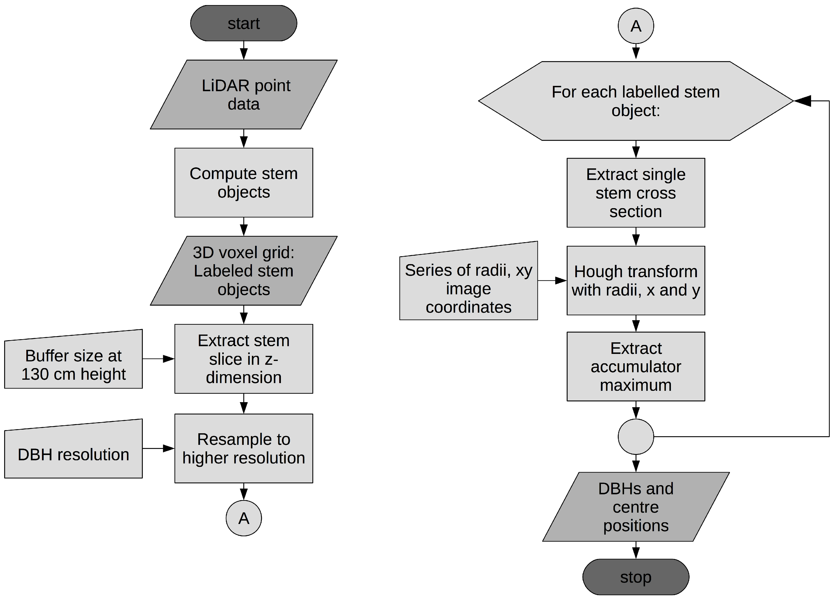
The estimation of tree stem diameter used and built up on priorly isolated tree stems from TLS-derived volumetric image data. For the isolation of the tree stems, techniques from 3D mathematical morphology were applied as described by Heinzel and Huber [12]. As an add-on method, DBH estimation required the single stem objects as input. Figure 1 gives an overview of the general procedure, starting with the extraction of tree stems from the original LiDAR point cloud. This first step included the transformation from point to 3D image data. The tree stems were compiled as connected components, constituting labelled objects of the voxel grid.
Following the stem isolation, a horizontal slice of the 3D stem image in the xy-plane was extracted with its vertical centre at 130 cm height. To determine the optimal thickness of the slice, a series of buffer sizes, starting from one voxel and up to a defined maximum, were tested. This ensured that a minimum buffer size could be determined, which was as tight as possible to the demanded height at 130 cm, but also covered stems being occluded at breast height. The optimal buffer size used for all of our plots had a thickness of four voxels, which corresponded to a height range from 120 to 140 cm and is slightly larger than the buffer used by Simonse et al. [22].
Depending on the scan data, the preceding tree stem isolation procedure has an optimal voxel size that usually is larger than the original voxel grid directly derived from the point cloud. This minimizes clumping effects and gaps between stem segments [12]. In the case of this study the original voxel grid had a resolution of 1 cm edge length, while the stem isolation was optimal at 5 cm [12]. In order to increase the precision of DBH estimation, the horizontal slice of the stem image was resampled to the maximum resolution of 1 cm. To receive the high resolution cross section, the coarse resolution stem slice was morphologically dilated with a disk shaped structuring element and intersected with the higher resolution data. The dilation effected the closing of gaps and buffering of the stem profile. At the end of this step, we retrieved a high resolution image slice containing the stem cross sections as labelled objects.
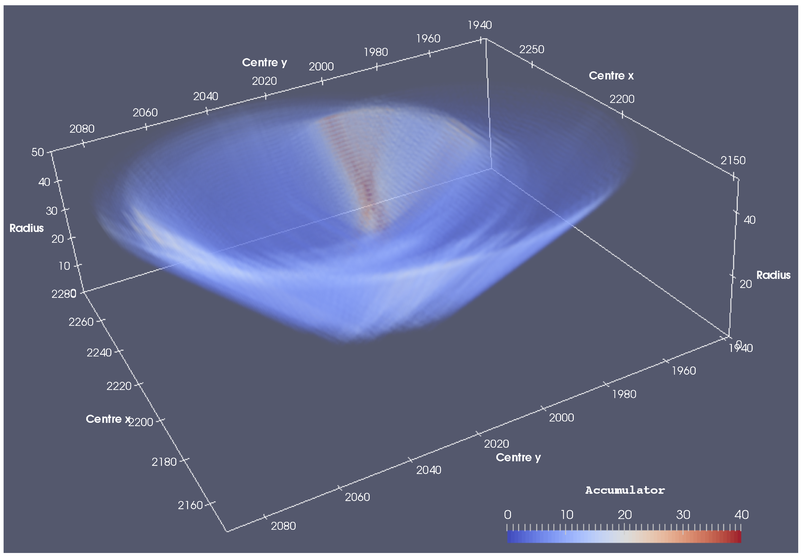
The prepared image slice was used in the core part of the procedure to estimate the stem diameters by Hough transforms of the image data. Hough transform for circle fitting optimizes the three parameters radius, x centre coordinate and y centre coordinate of the circle. Based on the binary cross section image, containing the potential circular structures, all possible centre locations are accumulated in parameter space [28,29,30]. Defining a set of n possible radii r, this accumulation contains all points at distances r with i = {1, 2, ..., n} to the related centre position. An example for the resulting 3D accumulator array is shown in Figure 2, where the accumulator values give an indication of how well a specific parameter combination describes circular structures in the original image. A more detailed description of Hough circle transforms can be found in the publications of Duda and Hart [30] and Yuen et al. [29]. For tree diameter estimation, we iteratively isolated each labelled stem profile in a single image, which subsequently was transformed into parameter space. The scheme of this subprocedure is illustrated in the right part of the flowchart in Figure 1. Parameter space was built with the set of radii on the z-axes and the x and y centre coordinates forming the x and y axis, respectively. The example in Figure 2 shows the parameter space of a single stem cross section image with 50 radii at 1 cm intervals. Due to the individual processing of each stem, the maximum accumulator value in parameter space defines the optimal set of circle parameters, from which stem DBH is the double radius. Final result of the iterative processing was a set with optimal DBH for each tree stem.
3.2. Accuracy Assessment
The results of the computed DBH were validated by comparing each tree with the field reference. The bias of the dataset was computed according to Equation (1) and the root mean square error (RMSE) after Equation (2). In both equations is the i-th reference DBH, is the i-th estimated DBH and n is the total number of stems.
In addition, the coefficient of determination () has been computed to denote the strength of the linear association between the estimated DBH and the reference DBH. has been computed after Equation (3), where is the mean of the observed diameters.
4. Results
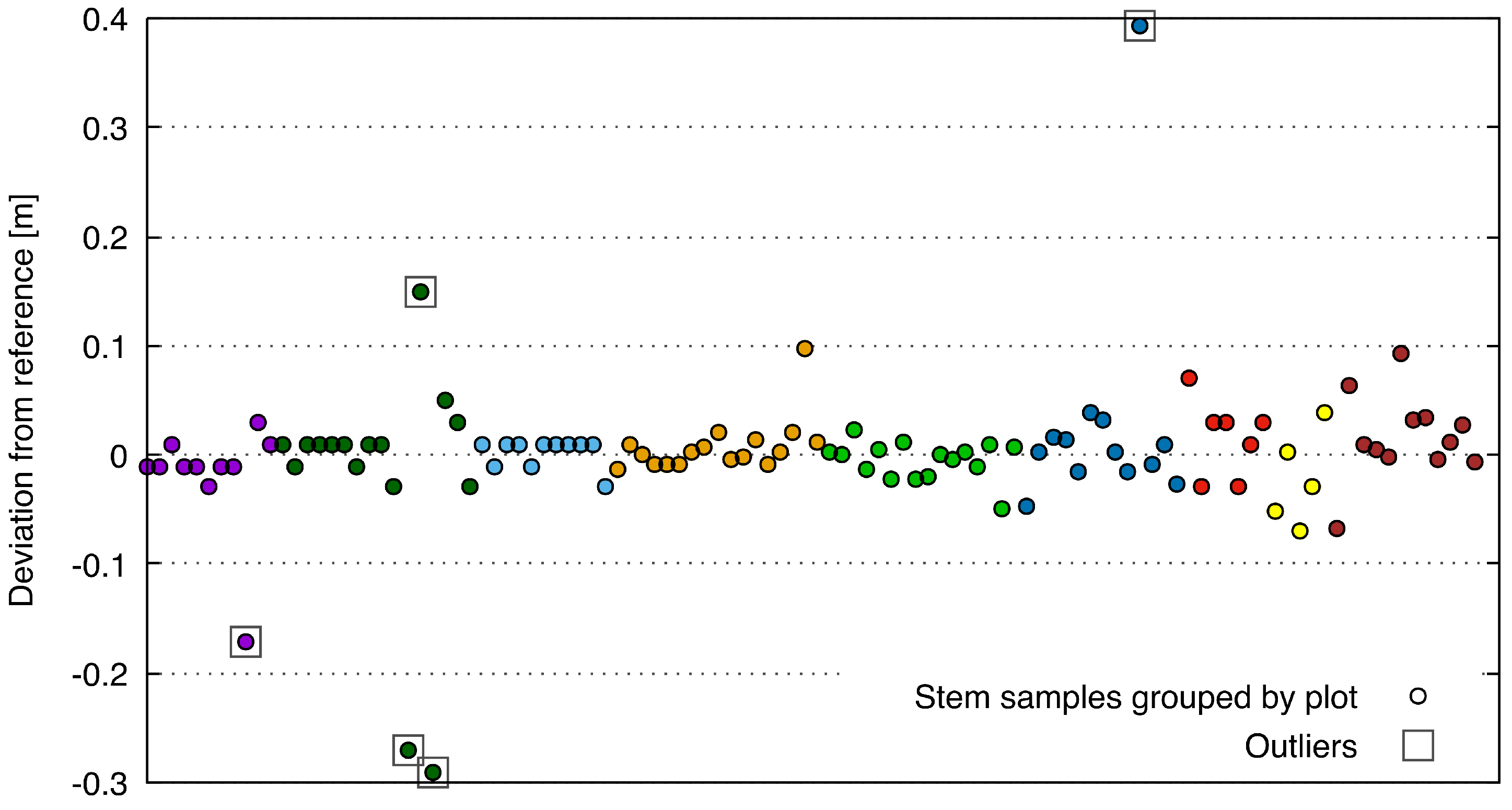
The diagram in Figure 3 plots the deviation of the DBH from the reference measurement for all tree stems separated by test site. For the complete dataset the bias amounted −0.1 cm and the RMSE 6.1 cm. From the same figure it can be seen that there exist five outliers, which are more than the double RMSE of 6.1 cm. They mostly resulted from registration inaccuracies or extreme occlusion and represent individual cases that are not systematic. Excluding them from the validation, finally resulted in a bias of only −0.02 cm and an RMSE of 2.9 cm.
When plotting the estimated DBH against the reference DBH in Figure 4 a strong linear association can be detected. Again, the linear relationship became even stronger when excluding the strongest outliers, which are marked with grey squares. Numerically this is expressed by an value that increased from 0.88 to 0.98. An overview of the statistical measures of the accuracy assessment is provided in Table 1.
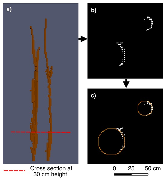
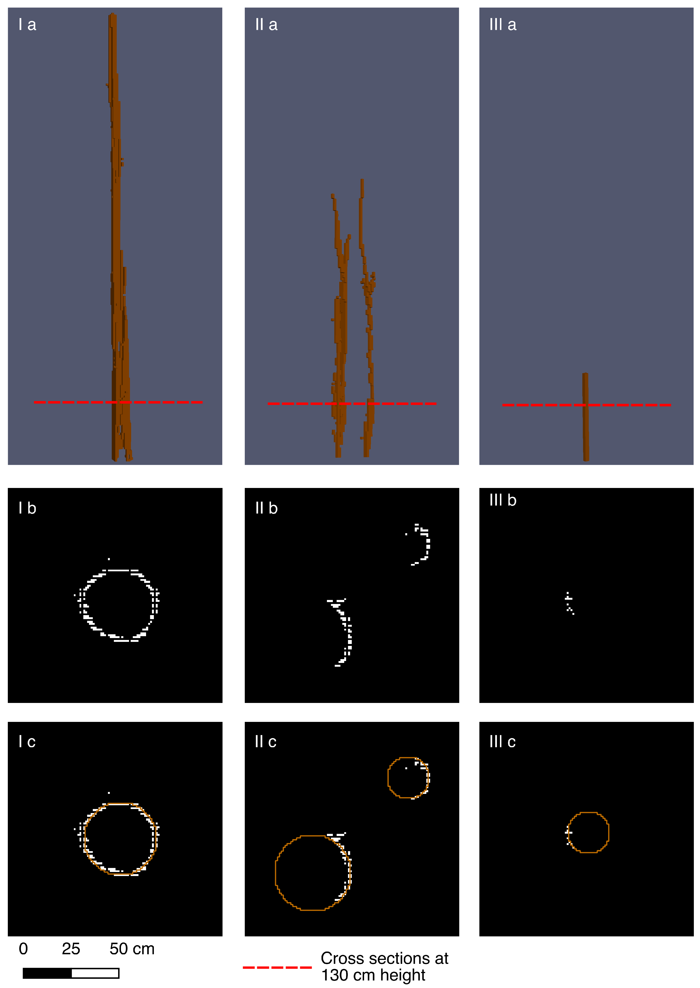
Visual inspection of the results by comparing stem cross sections revealed that the method worked well for different tree sizes and stem diameters, and also for cross sections, where only a very small fraction of the stem circumference was preserved in the laser scanning data. Figure 5 illustrates three examples of different stem sizes and for stem circumference profiles of varying completeness. Images (a) of all examples show the 3D volumetric image of the isolated tree stems; images (b) depict the high resolution cross section of the tree stems at breast height and images (c) show the circles fitted to the fragments of stem profiles. Example I covers a relatively tall tree with almost perfect stem profile in its cross section. Example II shows two medium sized trees, where laser scanning data contains slightly less than half of the stem profile in the cross section. The missing fractions of the stem profiles are due to occlusion and perspective effects. An even smaller fraction of the stem profile exists for the tree in example III. It can be seen that the method works properly, even for very small fragments of the stem profiles, as long as the curvature can be retrieved.
5. Discussion
The presented method introduced a procedure to estimate the DBH of tree stem objects obtained from 3D imagery. Results indicate good reliability of the computed DBH, so that it could generally substitute field based measurements. Deviations of the computed diameters to the reference measurements are less than 2 cm for most tree stems. It can be assumed that this order is within the accuracy of the tape based reference measurements taken in the field, which also include errors caused by bark structure, stem surface irregularities, the measurement tape not being exactly horizontally aligned around the stem and the actual measurement position deviating from exactly 1.3 m above ground. The varying number of influencing factors and the approximate range of error are also reflected by some studies investigating the accuracy of DBH field measurements. Luoma et al. inspected the DBH variance between field surveys of different mensurationists in a boreal forest while intentionally omitting the use of ambiguous references. They reported a standard deviation of 0.3 cm (1.5%) with 94% of the variation being below 1.5 cm and the maximum deviation amounting 2.1 cm [31]. Omule compared regular measurement practices of multiple workers against separate measurements, taken with additional precautions and used as references [32]. The variation of this experimental setting amounted 8.16% and 95% were within 5 cm of the reference. Besides the numeric results, we see the highest capacity of improvements for operational forestry related usage of TLS in the handling of multi-scan setups and their preprocessing.
The original dataset, including all stems, showed a low bias of only −0.1 cm, which is accompanied by a relatively high RMSE of 6.1 cm. The RMSE can be explained by the stronger influence of larger diameter deviations compared to smaller ones. Therefore, the exclusion of the five most outstanding outliers heavily reduced the RMSE to 2.9 cm and also the bias to 0.02 cm. In the present dataset, outliers mostly referred to scan registration inaccuracies or to extreme occlusion. Registration errors occurred when two or more scans were combined in one tree stem, but did not match precisely. Reasons for such matching imprecision can be diverse and do not necessarily have to be caused by technical errors. For example slight movements of the stems, caused by wind and during different scans, could induce difficulties with registration. This may result in stem cross sections, which do not show a clear curvature in order to fit circles correctly. In a few cases, extreme occlusion led to minimal fragments of cross section profiles that made circle fitting impossible.
Similar observations could be made for the value. While the value for the original and complete dataset of 0.88 already points to the reliability of the method, it further increased to 0.98 after exclusion of the extreme outliers. In addition, the almost constantly tight width of the sample distribution along the trend line in Figure 4 indicates, that the low error of the computed DBHs is largely independent from the stem diameter.
Methodological comparison of this study with other studies using Hough circle transforms, revealed principal differences. Most other studies applied Hough transform primarily for tree stem detection and derived the DBH only as a secondary product. Therefore, they transformed cross section images that included the original and unfiltered vegetation data. This approach causes problems, since the number of stems and circles to be fitted is unknown and must be limited by setting arbitrary thresholds, e.g., to the accumulator value. In this study the position and number of stems were acquired prior to DBH estimation. The Hough transform was applied to each stem individually with surrounding non-stem points being removed and allowed unambiguous estimation of a single and best fitting circle per stem.
One of the major and earliest studies on Hough transform for stem cross sections is from Simonse et al. [22], who used an undefined threshold to limit the number of fitted circles. The authors reported a bias for computed DBH of 1.7 cm, which is significantly higher than for our method. This might be explained by the coarse radius step sizes of 10 cm in parameter space applied in Simonse et al. [22], but also by the decrease in precision, when using the complete laser scanning vegetation data instead of prefiltered subsets for each stem. The studies of Aschoff et al. [23] and Thies and Spiecker [24] were based on the same method. Lindberg et al. [25] used Hough transforms to get a first approximation of the stem locations, but applied a different two-step approach when fitting circles for final estimation of the DBH. They reported a bias of 1.6 cm and a RMSE of 3.8 cm. Olofsen et al. [26] built up on a similar Hough transform based stem localisation, but used a RANSAC algorithm to extract the DBH. They achieved a bias of 1.3 cm and an RMSE of 5.9 cm.
Many studies exist, which estimate DBH with different methods than Hough transform. Examples for studies, which provided comparable accuracy metrics, are from Liang and Hyyppää [8], who reported on average a bias of 0.5 cm and a RMSE of 1.4 cm for their test sites, McDaniel et al. [6] with a median error of 9.8 cm and an RMSE of 13.2 cm and Maas et al. [20], who achieved a bias of 0.6 cm and a RMSE of 2.1 cm. values were reported by Kelbe et al. [9], who achieved a of 0.8 in combination with an RMSE of 6.4 cm and by Yao et al. [14] with an of 0.62 and an RMSE of 7.6 cm.
From the above, it can be seen that the concept of our method of applying Hough transform to priorly extracted stem objects provides very good results. The bias of the DBH and the are better than in other studies and when excluding the strongest individual outliers, both tend close towards their optimums that are almost no bias and a fully explained variation. The value of the RMSE is comparable to many other studies. Since it is influenced strongly by outliers, it improves to less than half of its original value, when removing the extreme outliers. However, the comparison between studies is not always clear, since experimental settings are often different and not always described sufficiently. Some studies, similarly to ours, reported DBH accuracies for datasets with outliers being removed [10,26]. Others used data from forest environments with less or without understory vegetation [15,20,25], which minimizes occlusion effects and simplifies stem extraction. Similar effects can be expected for studies from boreal forests with looser standing trees [7,8,26]. In contrast, our data originated from temperate mixed and coniferous forests with rich understory and occluded stems being the rule and not the exception.
6. Conclusions
Finally, it can be concluded that a precise method for DBH estimation could be applied on top of the results from stem detection. This DBH information complements the stem models of the new morphological stem detection approach and is an additional step towards further development of 3D-image-based methods. The accuracies of the results are better than of many other studies, which is an effect of using single priorly extracted stems with laser reflections from other vegetation parts being filtered out. For future, this method has the potential to substitute manual measurements of the DBH, as traditionally done by forest inventory. Major improvements for TLS-based methods in order to compete with traditional inventory practices, are still required in the automation and simplification of multi-scan workflows in the field and during preprocessing.
Acknowledgments
This study was conducted within the framework of the Swiss National Forest Inventory, a joint research program of the Swiss Federal Office for the Environment (FOEN) and the Swiss Federal Institute for Forest, Snow and Landscape Research (WSL). The authors would like to thank Natalia Rehush and Björn Dreier for their support in the fieldwork, Christian Ginzler for his expertise in GNSS technology and Susette Haegi for registration of the scans. Special thanks also go to the forest administration of the canton Grisons, Switzerland, who gave important assistance to this project.
Author Contributions
Johannes Heinzel conceived and developed the method, designed the fieldwork, and collected and processed the data. Markus O. Huber conceived and defined the main research objectives, designed the fieldwork, and managed the project. The manuscript was written by Johannes Heinzel with input from Markus O. Huber.
Conflicts of Interest
The authors declare no conflict of interest.
References
- Liang, X.; Kankare, V.; Hyyppä, J.; Wang, Y.; Kukko, A.; Haggrén, H.; Yu, X.; Kaartinen, H.; Jaakkola, A.; Guan, F.; et al. Terrestrial laser scanning in forest inventories. ISPRS J. Photogramm. Remote Sens. 2016, 115, 63–77. [Google Scholar] [CrossRef]
- Dorren, L.; Berger, F.; Jonsson, M.; Krautblatter, M.; Mölk, M.; Stoffel, M.; Wehrli, A. State of the art in rockfall—Forest interactions. Schweiz. Z. Forstwes. 2007, 158, 128–141. [Google Scholar] [CrossRef]
- Prandi, F.; Magliocchetti, D.; Poveda, A.; Amicis, R.D.; Andreolli, M.; Devigili, F. New Approach for forest inventory estimation and timber harvesting planning in mountain areas: The SLOPE project. Int. Arch. Photogramm. Remote Sens. Spat. Inf. Sci. 2016, XLI-B3, 775–782. [Google Scholar] [CrossRef]
- Stoffel, M.; Schneuwly, D.; Bollschweiler, M.; Lièvre, I.; Delaloye, R.; Myint, M.; Monbaron, M. Analyzing rockfall activity (1600–2002) in a protection forest—A case study using dendrogeomorphology. Geomorphology 2005, 68, 224–241. [Google Scholar] [CrossRef]
- Volkwein, A.; Schellenberg, K.; Labiouse, V.; Agliardi, F.; Berger, F.; Bourrier, F.; Dorren, L.K.A.; Gerber, W.; Jaboyedoff, M. Rockfall characterisation and structural protection—A review. Nat. Hazards Earth Syst. Sci. 2011, 11, 2617–2651. [Google Scholar] [CrossRef]
- McDaniel, M.W.; Nishihata, T.; Brooks, C.A.; Salesses, P.; Iagnemma, K. Terrain classification and identification of tree stems using ground-based LiDAR. J. Field Robot. 2012, 29, 891–910. [Google Scholar] [CrossRef]
- Liang, X.; Kankare, V.; Yu, X.; Hyyppa, J.; Holopainen, M. Automated Stem Curve Measurement Using Terrestrial Laser Scanning. IEEE Trans. Geosci. Remote Sens. 2014, 52, 1739–1748. [Google Scholar] [CrossRef]
- Liang, X.; Hyyppä, J. Automatic Stem Mapping by Merging Several Terrestrial Laser Scans at the Feature and Decision Levels. Sensors 2013, 13, 1614–1634. [Google Scholar] [CrossRef]
- Kelbe, D.; van Aardt, J.; Romanczyk, P.; van Leeuwen, M.; Cawse-Nicholson, K. Single-Scan Stem Reconstruction Using Low-Resolution Terrestrial Laser Scanner Data. IEEE J. Sel. Top. Appl. Earth Obs. Remote Sens. 2015, 8, 3414–3427. [Google Scholar] [CrossRef]
- Kankare, V.; Liang, X.; Vastaranta, M.; Yu, X.; Holopainen, M.; Hyyppä, J. Diameter distribution estimation with laser scanning based multisource single tree inventory. ISPRS J. Photogramm. Remote Sens. 2015, 108, 161–171. [Google Scholar] [CrossRef]
- Hackenberg, J.; Morhart, C.; Sheppard, J.; Spiecker, H.; Disney, M. Highly Accurate Tree Models Derived from Terrestrial Laser Scan Data: A Method Description. Forests 2014, 5, 1069–1105. [Google Scholar] [CrossRef]
- Heinzel, J.; Huber, M. Detecting Tree Stems from Volumetric TLS Data in Forest Environments with Rich Understory. Remote Sens. 2017, 9, 9. [Google Scholar] [CrossRef]
- Xia, S.; Wang, C.; Pan, F.; Xi, X.; Zeng, H.; Liu, H. Detecting stems in dense and homogeneous forest using single-scan TLS. Forests 2015, 6, 3923–3945. [Google Scholar] [CrossRef]
- Yao, T.; Yang, X.; Zhao, F.; Wang, Z.; Zhang, Q.; Jupp, D.; Lovell, J.; Culvenor, D.; Newnham, G.; Ni-Meister, W.; et al. Measuring forest structure and biomass in New England forest stands using Echidna ground-based lidar. Remote Sens. Environ. 2011, 115, 2965–2974. [Google Scholar] [CrossRef]
- Lovell, J.; Jupp, D.; Newnham, G.; Culvenor, D. Measuring tree stem diameters using intensity profiles from ground-based scanning lidar from a fixed viewpoint. ISPRS J. Photogramm. Remote Sens. 2011, 66, 46–55. [Google Scholar] [CrossRef]
- Vonderach, C.; Vögtle, T.; Adler, P.; Norra, S. Terrestrial laser scanning for estimating urban tree volume and carbon content. Int. J. Remote Sens. 2012, 33, 6652–6667. [Google Scholar] [CrossRef]
- Ravaglia, J.; Alexandra, B.; Piboule, A. Laser-scanned tree stem filtering for forest inventories measurements. In Proceedings of the 2013 IEEE Digital Heritage International Congress (DigitalHeritage), Marseille, France, 28 October–1 November 2013; pp. 649–652. [Google Scholar]
- Van Leeuwen, M.; Coops, N.C.; Newnham, G.J.; Hilker, T.; Culvenor, D.S.; Wulder, M.A. Stem detection and measuring DBH using terrestrial laser scanning. In Proceedings of the Silvilaser 2011, Hobart, Australia, 16–20 October 2011. [Google Scholar]
- Bienert, A.; Scheller, S.; Keane, E.; Mohan, F.; Nugent, C. Tree detection and diameter estimations by analysis of forest terrestrial laserscanner point clouds. Int. Arch. Photogramm. Remote Sens. Spat. Inf. Sci. 2007, XXXVI-3/W2, 50–55. [Google Scholar]
- Maas, H.G.; Bienert, A.; Scheller, S.; Keane, E. Automatic forest inventory parameter determination from terrestrial laser scanner data. Int. J. Remote Sens. 2008, 29, 1579–1593. [Google Scholar] [CrossRef]
- Henning, J.G.; Radtke, P.J. Detailed stem measurements of standing trees from ground-based scanning lidar. For. Sci. 2006, 52, 67–80. [Google Scholar]
- Simonse, M.; Aschoff, T.; Spiecker, H.; Thies, M. Automatic determination of forest inventory parameters using terrestrial laser scanning. In Proceedings of the Scandlaser Scientific Workshop on Airborne Laser Scanning of Forests, Umea, Sweden, 3–4 September 2003; pp. 252–258. [Google Scholar]
- Aschoff, T.; Thies, M.; Spiecker, H. Describing forest stands using terrestrial laser-scanning. Int. Arch. Photogramm. Remote Sens. Spat. Inf. Sci. 2004, 35, 237–241. [Google Scholar]
- Thies, M.; Spiecker, H. Evaluation and future prospects of terrestrial laser scanning for standardized forest inventories. Int. Arch. Photogramm. Remote Sens. Spat. Inf. Sci. 2004, XXXVI-8/W2, 192–197. [Google Scholar]
- Lindberg, E.; Holmgren, J.; Olofsson, K.; Olsson, H. Estimation of stem attributes using a combination of terrestrial and airborne laser scanning. Eur. J. For. Res. 2012, 131, 1917–1931. [Google Scholar] [CrossRef]
- Olofsson, K.; Holmgren, J.; Olsson, H. Tree Stem and Height Measurements using Terrestrial Laser Scanning and the RANSAC Algorithm. Remote Sens. 2014, 6, 4323–4344. [Google Scholar] [CrossRef]
- Zande, D.V.D.; Jonckheere, I.; Stuckens, J.; Verstraeten, W.W.; Coppin, P. Sampling design of ground-based lidar measurements of forest canopy structure and its effect on shadowing. Can. J. Remote Sens. 2008, 34, 526–538. [Google Scholar] [CrossRef]
- Davies, E. A modified Hough scheme for general circle location. Pattern Recognit. Lett. 1988, 7, 37–43. [Google Scholar] [CrossRef]
- Yuen, H.K.; Princen, J.; Dlingworth, J.; Kittler, J. A Comparative Study of Hough Transform Methods for Circle Finding. In Proceedings of the Fifth Alvey Vision Conference, Reading, UK, 25–28 September 1989. [Google Scholar]
- Duda, R.O.; Hart, P.E. Use of the Hough transformation to detect lines and curves in pictures. Commun. ACM 1972, 15, 11–15. [Google Scholar] [CrossRef]
- Luoma, V.; Saarinen, N.; Wulder, M.; White, J.; Vastaranta, M.; Holopainen, M.; Hyyppä, J. Assessing Precision in Conventional Field Measurements of Individual Tree Attributes. Forests 2017, 8, 38. [Google Scholar] [CrossRef]
- Omule, S.A. Personal bias in forest measurements. For. Chron. 1980, 56, 222–224. [Google Scholar] [CrossRef]
Figure 1.
Flowchart for estimating DBH from isolated 3D tree stem objects.

Figure 2.
3D parameter space transformed from a single tree stem cross section image. The three axis consist of the parameters x centre coordinate, y centre coordinate and radius. The maximum accumulator value defines the best circle fit.
Figure 2.
3D parameter space transformed from a single tree stem cross section image. The three axis consist of the parameters x centre coordinate, y centre coordinate and radius. The maximum accumulator value defines the best circle fit.

Figure 3.
Deviation of DBH from reference measurements for trees from nine independent plots. The samples are grouped by plot, of which each is separated by colour. Accuracy metrics were calculated with and without the marked outliers.
Figure 3.
Deviation of DBH from reference measurements for trees from nine independent plots. The samples are grouped by plot, of which each is separated by colour. Accuracy metrics were calculated with and without the marked outliers.

Figure 4.
Correlation between reference DBH and estimated DBH. The samples marked with squares are outliers. The coefficient of determination and the related linear model is given both for all stems and for the same dataset with outliers excluded.
Figure 4.
Correlation between reference DBH and estimated DBH. The samples marked with squares are outliers. The coefficient of determination and the related linear model is given both for all stems and for the same dataset with outliers excluded.

Figure 5.
Three examples (I)–(III) of circles fitted to tree stem cross sections covering different fractions of the original stem circumference. For all examples images (a) show the isolated 3D tree stem objects in the coarser resolution voxel grids; images (b) show the resampled higher resolution cross sections at 130 cm height and images (c) depict the circles fitted to the cross sections.


Table 1.
Overview of the verification results for the final dataset with outliers being excluded and the original dataset including all stems.
Table 1.
Overview of the verification results for the final dataset with outliers being excluded and the original dataset including all stems.
| Dataset | Bias [cm] | RMSE [cm] | |
|---|---|---|---|
| Outliers excluded | −0.02 | 2.9 | 0.98 |
| All stems | −0.1 | 6.1 | 0.88 |
© 2017 by the authors. Licensee MDPI, Basel, Switzerland. This article is an open access article distributed under the terms and conditions of the Creative Commons Attribution (CC BY) license (http://creativecommons.org/licenses/by/4.0/).
Share and Cite
MDPI and ACS Style
Heinzel, J.; Huber, M.O. Tree Stem Diameter Estimation From Volumetric TLS Image Data. Remote Sens. 2017, 9, 614. https://0-doi-org.brum.beds.ac.uk/10.3390/rs9060614
AMA Style
Heinzel J, Huber MO. Tree Stem Diameter Estimation From Volumetric TLS Image Data. Remote Sensing. 2017; 9(6):614. https://0-doi-org.brum.beds.ac.uk/10.3390/rs9060614
Chicago/Turabian StyleHeinzel, Johannes, and Markus O. Huber. 2017. "Tree Stem Diameter Estimation From Volumetric TLS Image Data" Remote Sensing 9, no. 6: 614. https://0-doi-org.brum.beds.ac.uk/10.3390/rs9060614
Note that from the first issue of 2016, this journal uses article numbers instead of page numbers. See further details here.