Four-Component Model-Based Decomposition for Ship Targets Using PolSAR Data

Abstract

Scattering mechanism (SM) analysis is a promising technique for ship detection and classification in polarimetric SAR (PolSAR) images. In this paper, a four-component model-based decomposition method incorporating surface, double-bounce, volume and cross-polarized components is proposed for analyzing the SMs of ships. A novel cross-polarized scattering component capable of discriminating between the HV scattering power generated by the oriented scatterers on ships from that by volume scatterers is proposed as a means to address the problem of volume scattering power overestimation. In the decomposition stage, by taking into account both the real and imaginary parts of the elements ${⟨\left[T\right]⟩}^{HV}(1,3)$ and ${⟨\left[T\right]⟩}^{HV}(2,3)$ of the observed coherency matrix, the proposed cross-polarized component can preserve the reflection asymmetry information completely, which is an essential property of man-made targets, such as ships. Based on the proposed decomposition method and an analysis of the different SMs between ships and sea clutter, a novel ship detection metric defined as $\mathbb{M}=ln\frac{P_d+P_c}{P_s}$ is proposed. Experimental results conducted on RadarSat-2 quad-polarimetric data validate the proposed four-component decomposition method as being more suitable for analyzing the SMs of ship targets than the existing helix matrix-based decomposition methods. Additionally, we find that the proposed ship detection metric can effectively enhance the signal-to-clutter ratio (SCR) and improve ship detection performance.

1. Introduction

Precise ship detection and classification are crucial for maritime security and environmental protection. Synthetic aperture radar (SAR) can provide wide-area, all-day and nearly all-weather observation and, as such, has played an important role in maritime ship surveillance [1]. Methods of ship detection and classification based on single-polarization SAR data have been extensively studied [2,3,4,5,6,7,8]. Recent technological trends involving SAR are moving towards the utilization of polarimetric SAR (PolSAR) data in this paper, we refer to fully-polarimetric or quad-polarimetric SAR data as polarimetric SAR (PolSAR) data). With PolSAR data containing more available information, e.g., amplitude and relative phase, than single-polarization SAR data, the scattering behavior of the ship target and sea clutter can be analyzed in detail. The methods of the classical polarimetric whitening filter (PWF) [9], polarimetric cross-entropy (PCE) [10], reflection symmetry analysis (RS) [11] and polarimetric notch filter (PNF) [12] can effectively reveal the difference in scattering behavior between the ship target and sea clutter and are widely utilized to separate ship targets from the surrounding sea clutter.

The model-based decomposition technique is one of the most popular and effective analytical methods employed in PolSAR data. Although primarily intended for land-cover classification, its ability to differentiate the scattering characteristics generated by the ship target from those by the sea surface makes it ideal for ship detection and classification. Wang et al. [13] adopted a classical Freeman and Durden three-component decomposition [14] method to investigate the scattering mechanisms (SMs) of different types of ships. They found that the main scattering of four types of ships, including hospital ships, landing platform docks (LPD), container ships and oil tankers, is volume scattering, but that hospital ships and LPDs have more surface scatterings, while oil tankers have more double-bounce scatterings. Sugimoto et al. [15] utilized a four-component model-based decomposition with orientation angle compensation proposed by Yamaguchi et al. [16] to analyze the scattering mechanisms of ships for the purpose of detection. They found that scattering from ships often consists of surface scattering, as well as considerable amounts of double-bounce and volume scattering. This difference between the SMs of the sea surface and ship targets allows for better detection of objects by designing discriminative detection metrics.

The classical Freeman and Durden three-component decomposition method assumes that the co-polarized (HH or VV) and cross-polarized (HV) channels are uncorrelated (i.e., $\langle S_{HH}{S}_{HV}^{*}\rangle \approx 0$ or $\langle S_{HV}{S}_{VV}^{*}\rangle \approx 0$). This assumption of reflection symmetry is satisfied in most natural distributed areas, but is not held by man-made structures such as ships. Hence, the three-component decomposition method is not suitable for analyzing the SMs of ships. Yamaguchi et al. [16,17] extended the three-component decomposition method by adding a helix scattering term to take into account the reflection asymmetric situation (i.e., $\langle S_{HH}{S}_{HV}^{*}\rangle \ncong 0$ or $\langle S_{HV}{S}_{VV}^{*}\rangle \ncong 0$). Although this method has demonstrated its effectiveness at separating the ship targets from the sea surface [15], several factors limit its ability to interpret the SMs of ship targets. First, this method assigns almost all HV scattering power to volume scattering, causing an overestimation of the volume scattering power. As mentioned in the literature [16,18,19,20], besides the volume scatterers, the oriented scatterers such as oriented dihedral corners and wires can also contribute to HV scattering power. Many attempts have been made to mitigate the overestimation of the volume scattering power: an effective way is to modify the volume scattering model so that it matches the real situation more reasonably [21,22,23]; another way is to generalize the odd- and double-bounce scattering models to take into account the HV scattering power generated by the oriented scatterers [24]. Second, the elements of the helix coherency matrix, i.e., $\langle \left[T_h\right]\rangle (2,3)$, comprise a pure imaginary number. This makes the helix coherency matrix incapable of accounting for the asymmetric information contained in the real part of the observed coherency matrix ${\langle \left[T\right]\rangle }^{HV}(2,3)$, which is often a complex number with a non-zero real part. The orientation angle compensation [16] can convert ${\langle {\left[T\right]}_r\rangle }^{HV}(2,3)$ into a pure imaginary number and make the observed coherency matrix match the helix matrix much better. However, a more reasonable solution would be one that could develop a more appropriate model to match the observation matrix, rather than the opposite. In addition, another reflection asymmetry term ${\langle {\left[T\right]}_r\rangle }^{HV}(1,3)$ related to the rotated coherency matrix is totally missed by the helix coherency matrix, causing a loss to measure the reflection asymmetry information of man-made targets.

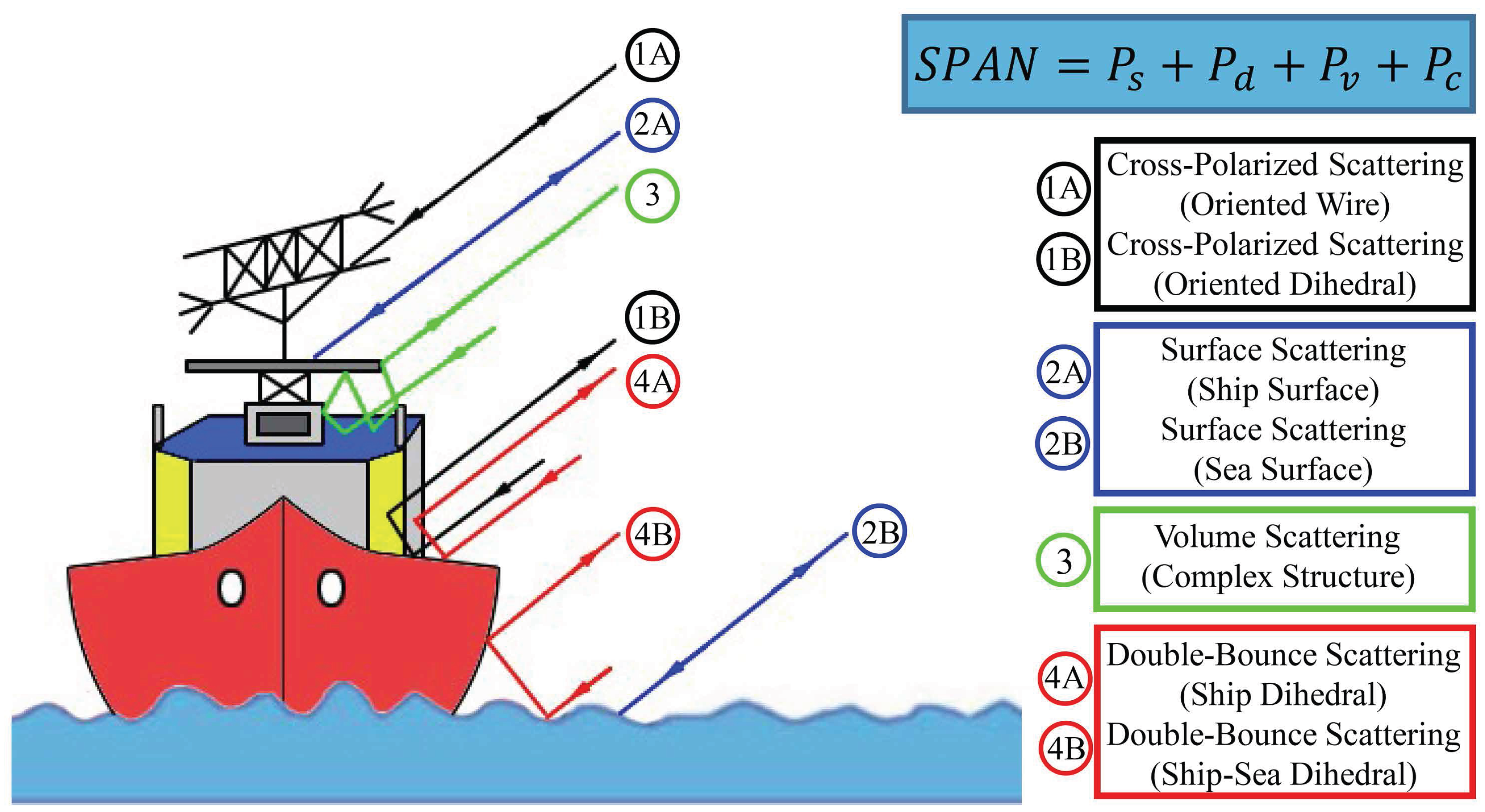
In this paper, to solve the existing problems and present a more accurate SM analysis of ships employed for detection and classification applications, we propose a four-component model-based decomposition method for ships in PolSAR data. The proposed model can effectively mitigate the overestimation of volume scattering power and present a complete description of the scattering asymmetry by incorporating a novel cross-polarized scattering component ($\langle {\left[T\right]}_c\rangle$) and a fine designed decomposition process. Specifically, as shown in Figure 1, a cross-polarized scattering component is proposed to model the HV scattering generated by the oriented scatterers, such as oriented dihedrals and wires on ships, to mitigate the overestimation of volume scattering power. This cross-polarized component can also describe the reflection asymmetry completely by taking into account both the real and imaginary parts of the elements ${\langle \left[T\right]\rangle }^{HV}(1,3)$ and ${\langle \left[T\right]\rangle }^{HV}(2,3)$ of the observed coherency matrix ${\langle \left[T\right]\rangle }^{HV}$ to retain the information lost by the helix matrix-based methods. The volume scattering component models the HV scattering power generated by the complicated superstructures on ships, barring the oriented scatterers, which are accounted for by the proposed cross-polarized component. Instead of using the traditional volume scattering component derived from randomly distributed dipoles to characterize the complex structures of ships, the coherency matrix with the maximal polarimetric entropy, i.e., the unit matrix proposed by An et al. [25], is used as the volume scattering model because of its ability to characterize the total randomness, which is the prime feature of volume scattering. The surface scattering component models the scattering generated by the sea surface and ship deck, etc., while the double-bounce scattering component is used to model scattering originating from dihedral corners such as broadside-sea configuration and deck-hatches on ships. Based on the proposed decomposition method and an analysis of the different SMs between ships and sea clutter, a novel ship detection metric defined as $\mathbb{M}=ln\frac{P_d+P_c}{P_s}$ is proposed. Experimental results conducted on RadarSat-2 quad-polarimetric data validate the proposed four-component decomposition method as being more suitable for analyzing the SMs of ship targets than the existing helix matrix-based decomposition methods. The proposed ship detection metric can effectively enhance the signal-to-clutter ratio (SCR) and improve ship detection performance significantly.

This paper is organized as follows. In Section 2, the proposed cross-polarized coherency component is described; then, the volume scattering component, the double-bounce and surface components are introduced, respectively. In Section 3, we introduce the proposed decomposition method in detail. The comprehensive experiments including SM analysis and ship detection conducted on RadarSat-2 PolSAR data are presented in Section 4.

2. Four-Component Scattering Model

2.1. Coherency Matrix

To interpret the polarimetric information contained in PolSAR data, the second-order statistics covariance or coherency matrix is preferred. In the backscattering case of mono-static PolSAR, according to the reciprocity, the 3D Pauli scattering vector ${\overrightarrow{k}}_p$ can be defined as:

$${\overrightarrow{k}}_p=\frac{1}{\sqrt{2}}{[S_{HH}+S_{VV},S_{HH}-S_{VV},2S_{HV}]}^{\mathcal{T}}$$

(1)

Then, the observed coherency matrix can be derived as:

$$\begin{array}{cc}{\langle \left[T\right]\rangle }^{HV}& ={\overrightarrow{k}}_p·{\overrightarrow{k}}_p^{{*}^{\mathcal{T}}}\\ & =\frac{1}{2}\left[\begin{array}{ccc}\langle {|S_{HH}+S_{VV}|}^2\rangle & \langle (S_{HH}+S_{VV}){(S_{HH}-S_{VV})}^{*}\rangle & \langle 2(S_{HH}+S_{VV})S_{HV}^{*}\rangle \\ \langle (S_{HH}-S_{VV}){(S_{HH}+S_{VV})}^{*}\rangle & \langle {|S_{HH}-S_{VV}|}^2\rangle & \langle 2(S_{HH}-S_{VV})S_{HV}^{*}\rangle \\ \langle 2S_{HV}{(S_{HH}+S_{VV})}^{*}\rangle & \langle 2S_{HV}{(S_{HH}-S_{VV})}^{*}\rangle & \langle 4{|S_{HV}|}^2\rangle \end{array}\right]\end{array}$$

(2)

where $\langle ·\rangle$ and superscripts $\mathcal{T}$, * denote ensemble average, transpose and complex conjugation, respectively. For simplicity, we rewrite the observed coherency matrix as:

$${\langle \left[T\right]\rangle }^{HV}=\left[\begin{array}{ccc}{T}_{11}& T_{12}& T_{13}\\ T_{21}& T_{22}& T_{23}\\ T_{31}& T_{32}& T_{33}\end{array}\right]$$

(3)

2.2. Cross-Polarized Scattering Model

The cross-polarized scattering matrix proposed by Moriyama et al. [18] is defined as:

$${\left[S\right]}^{HV}=\left[\begin{array}{cc}\gamma & \rho \\ \rho & 1\end{array}\right]$$

(4)

where $\gamma$ and $\rho$ are ratios of HH and HV backscattering to VV, respectively; where,

$$\gamma =\frac{S_{HH}}{S_{VV}}\rho =\frac{S_{HV}}{S_{VV}}$$

(5)

Any scatterer with a certain orientation angle can produce HV scattering power, resulting in a non-zero $\rho$; thus, the cross-polarized scattering matrix can be used to measure the HV scattering produced by the oriented scatterers on ships. Although the horizontal and vertical scatterers such as dihedral corners and wires are reflection symmetric, most of them are oriented at different angles with a non-uniform distributions, making ships’ reflection asymmetric. To describe the asymmetric scattering information of ships quantitatively, we consider the average contribution of several scatterers by mathematical integration. Now, let us assume that the scatterers are oriented about the radar look direction at angle $\theta$ from the vertical polarization direction; the oriented cross-polarized scattering matrix becomes:

$${\left[S\right]}^{hv}=\left[\begin{array}{cc}{S}_{hh}& S_{hv}\\ S_{vh}& S_{vv}\end{array}\right]=\left[\begin{array}{cc}\cos \theta & \sin \theta \\ -\sin \theta & \cos \theta \end{array}\right]\left[\begin{array}{cc}\gamma & \rho \\ \rho & 1\end{array}\right]\left[\begin{array}{cc}\cos \theta & -\sin \theta \\ \sin \theta & \cos \theta \end{array}\right]$$

(6)

Specifically, the elements are:

$$\begin{array}{cc}\hfill S_{hh}& =\rho ·\sin 2\theta +{\sin }^2\theta +\gamma ·{\cos }^2\theta \hfill \\ \hfill S_{hv}& =\rho ·\cos 2\theta +\frac{1}{2}(1-\gamma )·\sin 2\theta \hfill \\ \hfill S_{vv}& =\gamma ·{\sin }^2\theta -\rho ·\sin 2\theta +{\cos }^2\theta \hfill \end{array}$$

(7)

Similarly, we parameterize the proposed cross-polarized coherency as Equation (8). The mathematical forms of the elements of the cross-polarized coherency are derived via integration using a probability density function $p\left(\theta \right)$ [21] with its peak at zero degrees (see Equation (9)), and any of the expected values can be derived using similar operations with Equation (10):

$$\langle {\left[T\right]}_c\rangle =\left[\begin{array}{ccc}{T}_{c11}& T_{c12}& T_{c13}\\ T_{c21}& T_{c22}& T_{c23}\\ T_{c31}& T_{c32}& T_{c33}\end{array}\right]$$

(8)

$$p\left(\theta \right)=\frac{1}{2}\cos \theta ,[-\frac{1}{2}\pi ,\frac{1}{2}\pi ]$$

(9)

$$\langle |S_{hh}+S_{vv}{|}^2\rangle ={\int }_{-\frac{1}{2}\pi }^{\frac{1}{2}\pi }(S_{hh}+S_{vv})·{(S_{hh}+S_{vv})}^{*}·p\left(\theta \right)d\theta$$

(10)

The elements of the proposed cross-polarized coherency are in the formulas:

$$\begin{array}{cc}\hfill T_{c11}& =\frac{1}{2}\langle |S_{hh}+S_{vv}{|}^2\rangle =\frac{1}{2}{|\gamma |}^2+{\gamma }_{re}+\frac{1}{2}\hfill \end{array}$$

(11a)

$$\begin{array}{cc}\hfill T_{c22}& =\frac{1}{2}\langle |S_{hh}-S_{vv}{|}^2\rangle =\frac{7}{30}{|\gamma |}^2-\frac{7}{15}{\gamma }_{re}+\frac{16}{15}{|\rho |}^2+\frac{7}{30}\hfill \end{array}$$

(11b)

$$\begin{array}{cc}\hfill T_{c33}& =\langle 2|S_{hv}{|}^2\rangle =\frac{4}{15}{|\gamma |}^2-\frac{8}{15}{\gamma }_{re}+\frac{14}{15}{|\rho |}^2+\frac{4}{15}\hfill \end{array}$$

(11c)

$$\begin{array}{cc}\hfill T_{c12}& =\frac{1}{2}\langle (S_{hh}+S_{vv}){(S_{hh}-S_{vv})}^{*}\rangle =\frac{1}{6}(\gamma +1)({\gamma }^{*}-1)\hfill \end{array}$$

(11d)

$$\begin{array}{cc}\hfill T_{c13}& =\langle (S_{hh}+S_{vv})S_{hv}^{*}\rangle =\frac{16+5\pi }{40}{\rho }^{*}(\gamma +1)\hfill \end{array}$$

(11e)

$$\begin{array}{cc}\hfill T_{c23}& =\langle (S_{hh}-S_{vv})S_{hv}^{*}\rangle =\frac{8}{15}\rho (1-{\gamma }^{*})+\frac{16-5\pi }{40}{\rho }^{*}(\gamma -1)\hfill \end{array}$$

(11f)

where ${\gamma }_{re}$ represents the real part of $\gamma$. It is worth noting that both $T_{c13}$ and $T_{c23}$ have a certain complex value, and their real part is not always equal to zero. Since $\langle (S_{HH}+S_{VV})S_{HV}^{*}\rangle \ncong 0$ and $\langle (S_{HH}-S_{VV})S_{HV}^{*}\rangle \ncong 0$ of the observed coherency represent the reflection asymmetry, Equation (11e,f) indicates that the proposed cross-polarized coherency matrix can be used to take account of the reflection asymmetry completely. In addition, as the proposed coherency is derived from the cross-polarized scattering matrix, it can be also used to measure the cross-polarized scattering power produced by oriented dihedrals and oriented wires.

It should be noted that the orientation compensation widely used in the previous method [16,25] should not be applied to the observed coherency matrix because the orientation information is the basis of the cross-polarized coherency [24].

2.3. Volume Scattering Model

The traditional volume scattering component is derived from randomly-oriented dipoles and is suitable for measuring the HV scattering from forests. When it comes to ship targets, it seems that these volume models do not match the observed data because there are few oriented dipoles on ships. Generally, the volume scatterer is a considerably complicated structure, the scattering from which can be regarded as a combination of several kinds of SMs. As a result, the polarimetric entropy of the volume scattering should be high. Based on the above analysis, we adopt the coherency matrix with the maximal polarimetric entropy, which is, i.e., the unit matrix (see Equation (12)) proposed by An et al. [25], to model the volume scattering power retained after the cross-polarized scattering power corresponding to the oriented scatterers is subtracted.

$$\langle {\left[T\right]}_v\rangle =\left[\begin{array}{ccc}1& 0& 0\\ 0& 1& 0\\ 0& 0& 1\end{array}\right]$$

(12)

2.4. Double-Bounce and Surface Scattering Model

The double-bounce scattering component models the scattering from a dihedral corner reflector, such as the ship side-sea surface, deck-hatches and other dihedral structures on ships. The surface scattering component models the scattering from first-order Bragg surfaces (sea surface) and planes (ship deck). Following [26], the coherency matrices for double-bounce and surface components are given as Equations (13) and (14), respectively:

$$\langle {\left[T\right]}_d\rangle =\left[\begin{array}{ccc}{|\alpha |}^2& \alpha & 0\\ {\alpha }^{*}& 1& 0\\ 0& 0& 0\end{array}\right]$$

(13)

$$\langle {\left[T\right]}_s\rangle =\left[\begin{array}{ccc}1& {\beta }^{*}& 0\\ \beta & {|\beta |}^2& 0\\ 0& 0& 0\end{array}\right]$$

(14)

where $\alpha$ and $\beta$ are complex numbers.

3. Decomposition Method

When analyzing the SMs of ships, we have two basic elements of a priori domain knowledge: (1) Ships are constructed mainly by planes, dihedral corners and a few volume scatterers with complicated structures. As a result, ships should be surface and double-bounce scattering dominated, while the volume scattering power should not be high in general. In addition, besides the volume scatterers, the oriented scatterers on ships such as oriented dihedral corners and wires can also generate HV scattering; hence, the HV scattering power corresponding to volume scatterers on ships should be low. (2) Reflection symmetry is a powerful tool by which the essential difference between ship targets and sea clutter can be characterized [27]. The natural sea background scenario possesses symmetry properties, while such properties no longer apply with man-made metallic targets, i.e., ships at sea. In practice, the reflection asymmetry-related components, such as a helix matrix, are usually adopted to measure the symmetry property of the given object. If the normalized power (which is defined as the corresponding decomposition power divided by the total backscattered power, i.e., $SPAN$) of the reflection asymmetric component is close to zero, the object under test is regarded as a reflection symmetric target; if the normalized power is close to one, the given object is a non-reflection symmetric target. Keeping these two rationales in mind, we expand the observed coherency matrix ${\langle \left[T\right]\rangle }^{HV}$ as Equation (15) by using the four components described above, i.e., the proposed cross-polarized coherency matrix, the unit matrix with the maximal polarimetric entropy and the coherency matrix corresponding to the surface and double-bounce scatterers.

$$\begin{array}{cc}\hfill {\langle \left[T\right]\rangle }^{HV}& =f_s\langle {\left[T\right]}_s\rangle +f_d\langle {\left[T\right]}_d\rangle +f_v\langle {\left[T\right]}_v\rangle +f_c\langle {\left[T\right]}_c\rangle \hfill \\ & =f_s\left[\begin{array}{ccc}1& {\beta }^{*}& 0\\ \beta & {|\beta |}^2& 0\\ 0& 0& 0\end{array}\right]+f_d\left[\begin{array}{ccc}{|\alpha |}^2& \alpha & 0\\ {\alpha }^{*}& 1& 0\\ 0& 0& 0\end{array}\right]+f_v\left[\begin{array}{ccc}1& 0& 0\\ 0& 1& 0\\ 0& 0& 1\end{array}\right]+f_c\left[\begin{array}{ccc}{T}_{c11}& T_{c12}& T_{c13}\\ T_{c21}& T_{c22}& T_{c23}\\ T_{c31}& T_{c32}& T_{c33}\end{array}\right]\hfill \end{array}$$

(15)

where the cross-polarized coherency matrix $\langle {\left[T\right]}_c\rangle$ can be obtained by Equation (11) and $f_s$, $f_d$, $f_v$, $f_c$, $\alpha$ and $\beta$ are six parameters that need to be determined. Now, comparing the left-hand with the right-hand side of Equation (15), we have the following six basic equations:

$$\begin{array}{cc}\hfill T_{11}& =f_s+f_d{|\alpha |}^2+f_c{T}_{c11}+f_v\hfill \end{array}$$

(16a)

$$\begin{array}{cc}\hfill T_{22}& =f_s{|\beta |}^2+f_d+f_c{T}_{c22}+f_v\hfill \end{array}$$

(16b)

$$\begin{array}{cc}\hfill T_{33}& =f_c{T}_{c33}+f_v\hfill \end{array}$$

(16c)

$$\begin{array}{cc}\hfill T_{12}& =f_s{\beta }^{*}+f_d\alpha +f_c{T}_{c12}\hfill \end{array}$$

(16d)

$$\begin{array}{cc}\hfill T_{13}& =f_c{T}_{c13}\hfill \end{array}$$

(16e)

$$\begin{array}{cc}\hfill T_{23}& =f_c{T}_{c23}\hfill \end{array}$$

(16f)

Equation (16e,f) can give two different coefficients $f_c$, of which only one is needed. In this paper, we empirically average their values in order to fully utilize the information provided by the observed matrix ${\langle \left[T\right]\rangle }^{HV}$ and derive the resulting $f_c$ as:

$$f_c=\frac{1}{2}\left|\frac{T_{13}}{T_{c13}}+\frac{T_{23}}{T_{c23}}\right|$$

(17)

then $f_v$ is derived from Equation (16c) as:

$$f_v=T_{33}-f_c{T}_{c33}$$

(18)

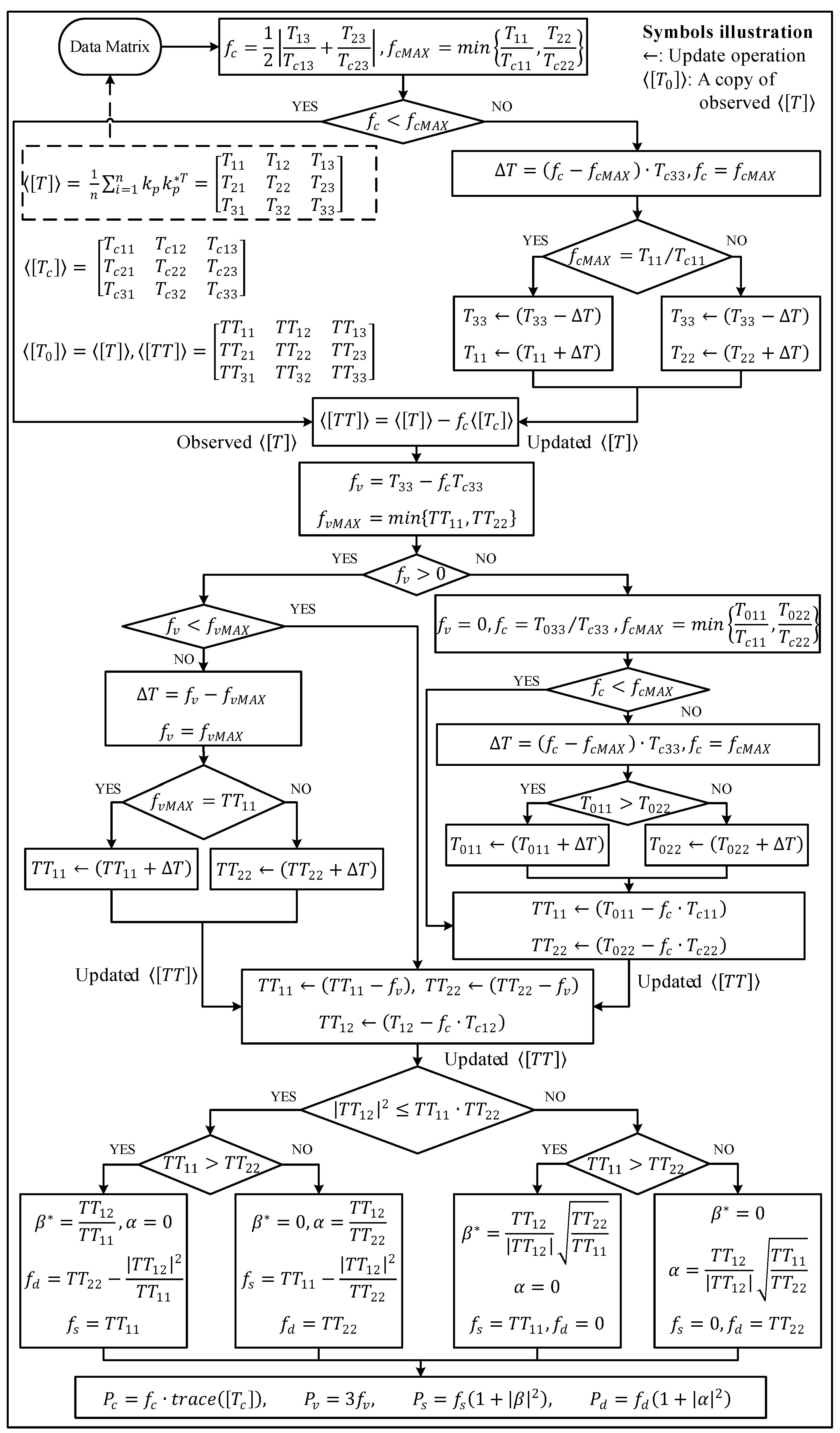
The proposed cross-polarized component is reflection symmetry related. We utilize this component to measure whether the given object is reflective symmetric or reflective asymmetric. Thus, the cross-polarized component should always exist in the decomposition process. Based on this rationale, if $f_v\le 0$ occurs, the volume scattering component rather than the cross-polarized component will be removed, i.e., $f_v$ is set to zero, and the four-component decomposition is automatically converted to a three-component decomposition. After $f_c$ and $f_v$ are obtained, the remaining four parameters can be derived following [25]. To ensure that $f_s$ and $f_d$ are non-negative, the power constraint is also incorporated. Basically, if either $f_c$ or $f_v$ exceeds its maximum, we re-assign it to its maximum. The re-assignment of $f_c$ or $f_v$ may break the power balance between the real total backscattered power $SPAN$ and the summation of the power of four decomposed components; thus, such problems should be handled carefully. The detailed flowchart of the proposed decomposition process is shown in Figure 2. The final power corresponding to the four components is derived as:

$$\begin{array}{cc}\hfill P_s& =f_s{(1+|\beta |}^2)\hfill \\ \hfill P_d& =f_d{(1+|\alpha |}^2)\hfill \\ \hfill P_v& =3f_v\hfill \\ \hfill P_c& =f_c·trace\left(\langle {\left[T\right]}_c\rangle \right)\hfill \end{array}$$

(19)

under the constraint of:

$$SPAN=P_s+P_d+P_v+P_c$$

(20)

where $trace(·)$ denotes the trace of a matrix. Equations (15)–(20) are the main set of expressions for the four-component decomposition.

4. Experimental Results and Discussion

4.1. SAR Data and Comparative Methods

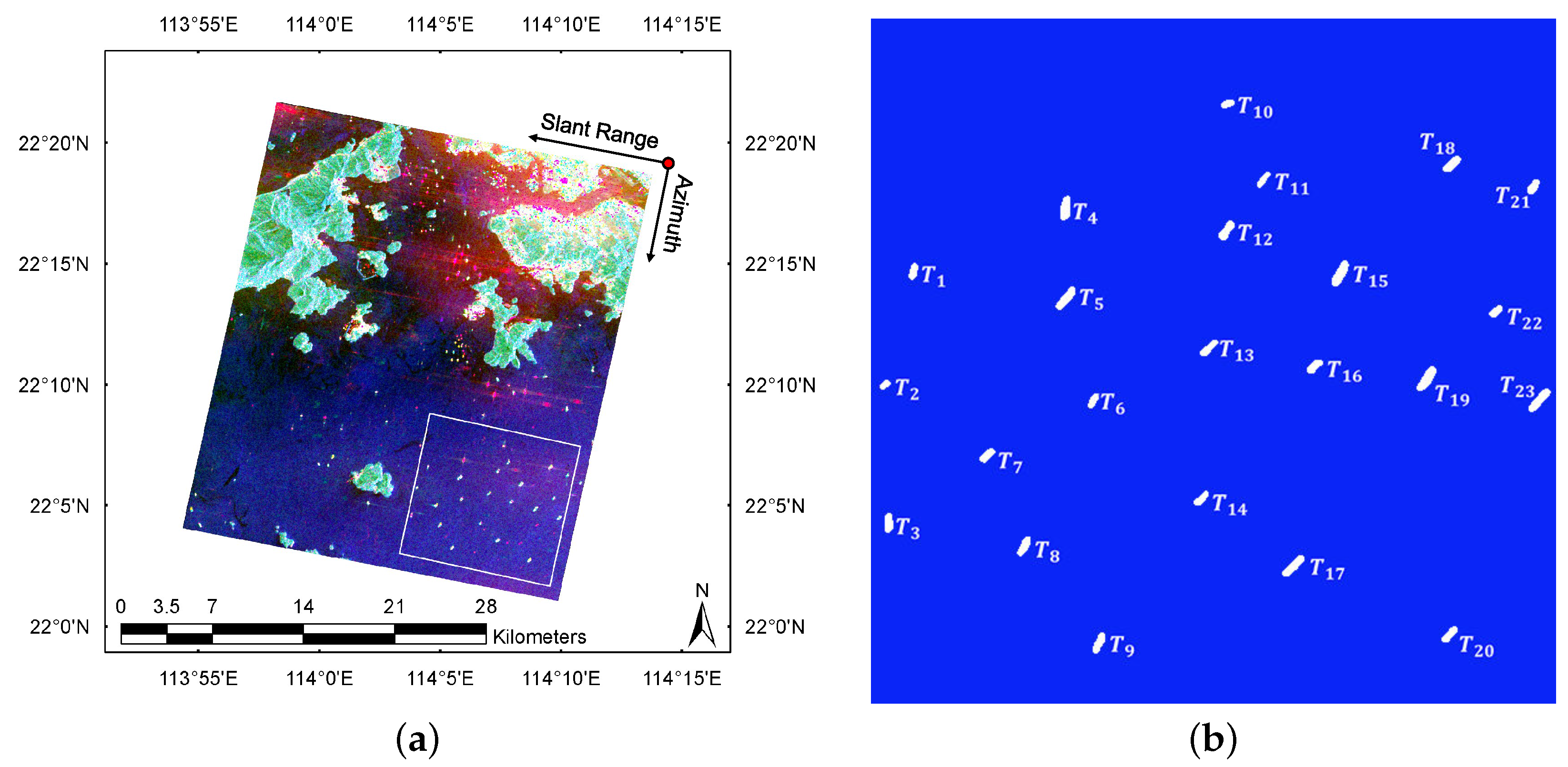
As shown in Figure 3, C-band RadarSat-2 polarimetric data acquired on 16 December 2008 over the Hong Kong area were used to validate the proposed four-component model-based decomposition method. The mean incident angle is $28.{97}^{\circ }$. At the time of SAR data acquisition, the sea was at low to medium wave. We multilooked the data by four look-numbers in the azimuth direction and two look-numbers in the range direction, which corresponds to about 10 m × 10 m on the ground. Then, mean filtering with a window size of $5\times 5$ was used to reduce the speckle noise. To focus on the scattering analysis of ship targets, a sub-area marked by the blue rectangle in Figure 3a was selected for our experiments. Figure 3b represents the ground truth of ship locations and complete contours obtained by the expert interpreter. In this figure, all pixels belonging to ships are colored in white. The ships are numbered to facilitate convenient reference in the following sections.

Two existing representative methods S4R, C4G and an improved method IC4G were compared with the proposed method P4C

• S4R: a four-component decomposition method developed by Sato et al. [21] that incorporates the matrix rotation and extended volume scattering model. The matrix rotation leads to $Re\left\{T_{23}\right\}=0$ and minimizes the cross-polarized power ($T_{33}$) generated by dipole scattering plus dihedral scattering. The extended volume scattering model is used to account for the HV scattering power generated by the oriented structures.
• C4G: a four-component decomposition method proposed by Chen [24] that generalizes the odd- and double-bounce scattering models to fit the cross-polarization and off-diagonal terms by separating their independent orientation angles. A general decomposition framework is proposed that utilizes all elements of a coherency matrix. The residual minimization criterion is used for model inversion.
• IC4G: The original C4G has nine equations (refer to Equation (27) in [24]), but ten unknown parameters if the imaginary part of $\beta$ is considered. To make the nonlinear least squares optimization problem have a determined solution, Chen et al. neglected the imaginary part of $\beta$ considering that $\beta$ can be approximated as a real value for most natural surfaces. However, as mentioned earlier, the imaginary part of $\beta$ should be considered to improve the decomposition accuracy. In order to satisfy a determined equation system when considering the imaginary part of $\beta$, an improved version is herein proposed that contains the additional constraint that $SPAN$ equals the total power of four components. With this additional equation, we can obtain all of those ten parameters following the original decomposition framework.
• P4C: the proposed four-component decomposition method for ships. It has the ability to discriminate HV scattering power generated by oriented scatterers from that by volume scatterers to mitigate the volume scattering power overestimation. It also emphasizes that the reflection asymmetry term should exist in all cases and takes both real and imaginary parts of ${\langle \left[T\right]\rangle }^{HV}(1,3)$ and ${\langle \left[T\right]\rangle }^{HV}(2,3)$ of the observed coherency matrix ${\langle \left[T\right]\rangle }^{HV}$ into account to measure the reflection asymmetry completely.

4.2. Analysis of the Ship Scattering Mechanism

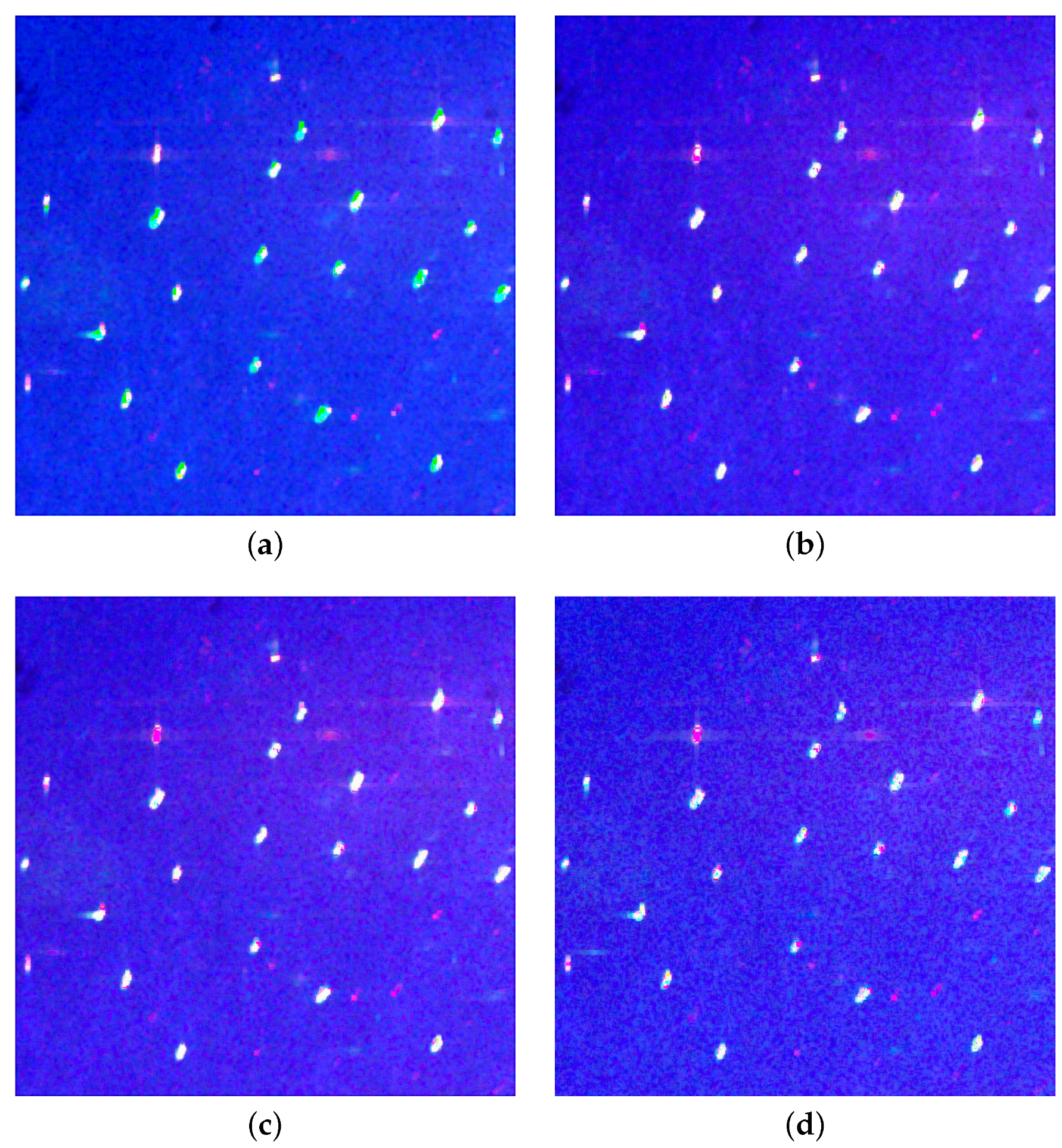
In this section, we evaluate the capability of comparative methods to reveal the SMs of ships. With the above-mentioned four-component decomposition methods, each pixel in PolSAR data will get four power measurements, i.e., $P_d$, $P_v$, $P_s$ and $P_c$ for the proposed method P4C or $P_d$, $P_v$, $P_s$ and $P_h$ for the other three methods S4R, C4G and IC4G. In order to provide a visual comparison for different methods, the $P_d$, $P_v$ and $P_s$ were assigned red, green and blue, respectively. Then, we combined $P_d$, $P_v$, $P_s$ to generate an RGB image, as shown in Figure 4, to analyze the SMs of ships. From the comparative subplots, we find that in most cases, all methods present satisfactory decomposition results for sea clutter, which appears blue, indicating that the surface scattering power ($P_s$) is the major contributor of the four components. For ship targets, we find that many ships in Figure 4a corresponding to the result of S4R appear green, indicating that the volume scattering component contributes more than other components. This is not consistent with the a priori domain knowledge of ships. As analyzed in [6,15], a ship is mainly composed of surface or double-bounce scatterers, such as decks, cabins and guardrails. In contrast, only a few complicated superstructures on the ship contribute to volume scattering. Therefore, generally speaking, for ship targets, either surface or double-bounce scattering, not volume scattering, should dominate. The result shown in Figure 4a indicates that the method of S4R overestimates the volume scattering power of ships to some degree. Visually, all of the other three methods, including the original C4G (Figure 4b), the improved IC4G (Figure 4c) and the proposed P4C (Figure 4d), outperform S4R in terms of mitigating the overestimation of volume scattering.

To facilitate a quantitative evaluation of the performances of different decomposition methods, based on the ground truth image as shown in Figure 3b, which was obtained by an expert interpreter, the powers of different components are averaged for ship and sea clutter pixels, respectively. The detailed decomposition component power distribution statistics are listed in

Table 1. Distributions of scattering components with different decompositions.

	Ships					Sea
	$\mathit{P}4\mathit{C}$	$\mathit{IC}4\mathit{G}$	$\mathit{C}4\mathit{G}$	$\mathit{S}4\mathit{R}$		$\mathit{P}4\mathit{C}$	$\mathit{IC}4\mathit{G}$	$\mathit{C}4\mathit{G}$	$\mathit{S}4\mathit{R}$
Cross or Helix ${}^{†}$	17.52%	4.18%	4.09%	3.96%		2.61%	0.25%	0.28%	0.29%
Double-bounce	18.11%	25.04%	27.54%	21.16%		2.35%	5.34%	5.36%	2.33%
Surface	50.33%	49.15%	43.89%	39.62%		93.51%	91.63%	91.36%	93.47%
Volume	14.04%	21.63%	24.48%	35.26%		1.54%	2.78%	3.00%	3.91%
Power Difference ${}^{‡}$	0.00%	−0.08%	−0.15%	0.08%		0.00%	0.41%	0.41%	0.42%

Notes: ${}^{†}$ Calculated by $P_c/(P_c+P_s+P_d+P_v)\ast 100\%$ and the same way with the other components; ${}^{‡}$ calculated by $(SPAN-(P_c+P_s+P_d+P_v))/SPAN\ast 100\%$.

. It is seen that the volume scattering power of ships is $35.26\%$ for S4R, which is regarded as an overestimation, and $24.48\%$ for C4G. That is to say, the overestimation of the volume scattering power for ships is mitigated significantly by C4G. The volume scattering power is decreased further by IC4G to $21.63\%$. The proposed method of P4C achieved the lowest average volume scattering power $14.04\%$. Considering the real distribution of superstructures on ships [6], this result is reasonable. It also should be noted that the volume scattering power depends on the type of ship. A volume scattering component contributing for about $14\%$ to the $SPAN$ could be reasonable for some kinds of ships, but it can be an over-/under-estimation for other types of ships. In addition, it is seen that except for the proposed method, the other three methods suffer from the problem of power differences, i.e., the summation of all of the power components is not equal to the actual total power $SPAN$. By introducing a total power constraint in the proposed decomposition strategy, as shown in Figure 2, this power difference has been eliminated. For the purpose of solving all ten parameters, the power constraint is also used by IC4G. However, because IC4G applies an optimization algorithm based on the residual minimization criterion, the possible local optimal solution also leads to power differences.

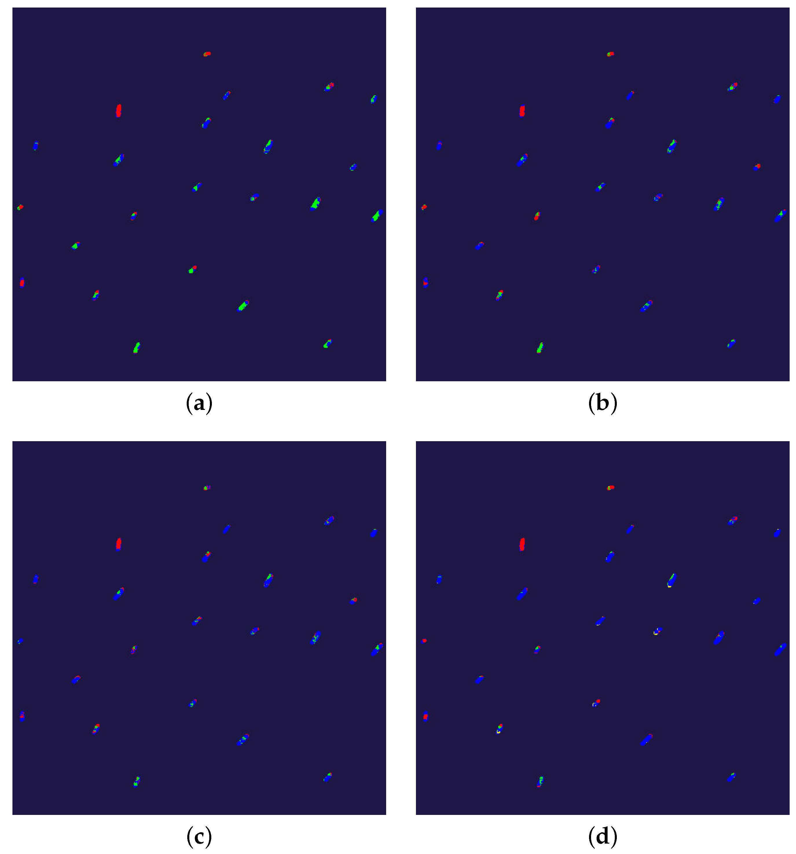
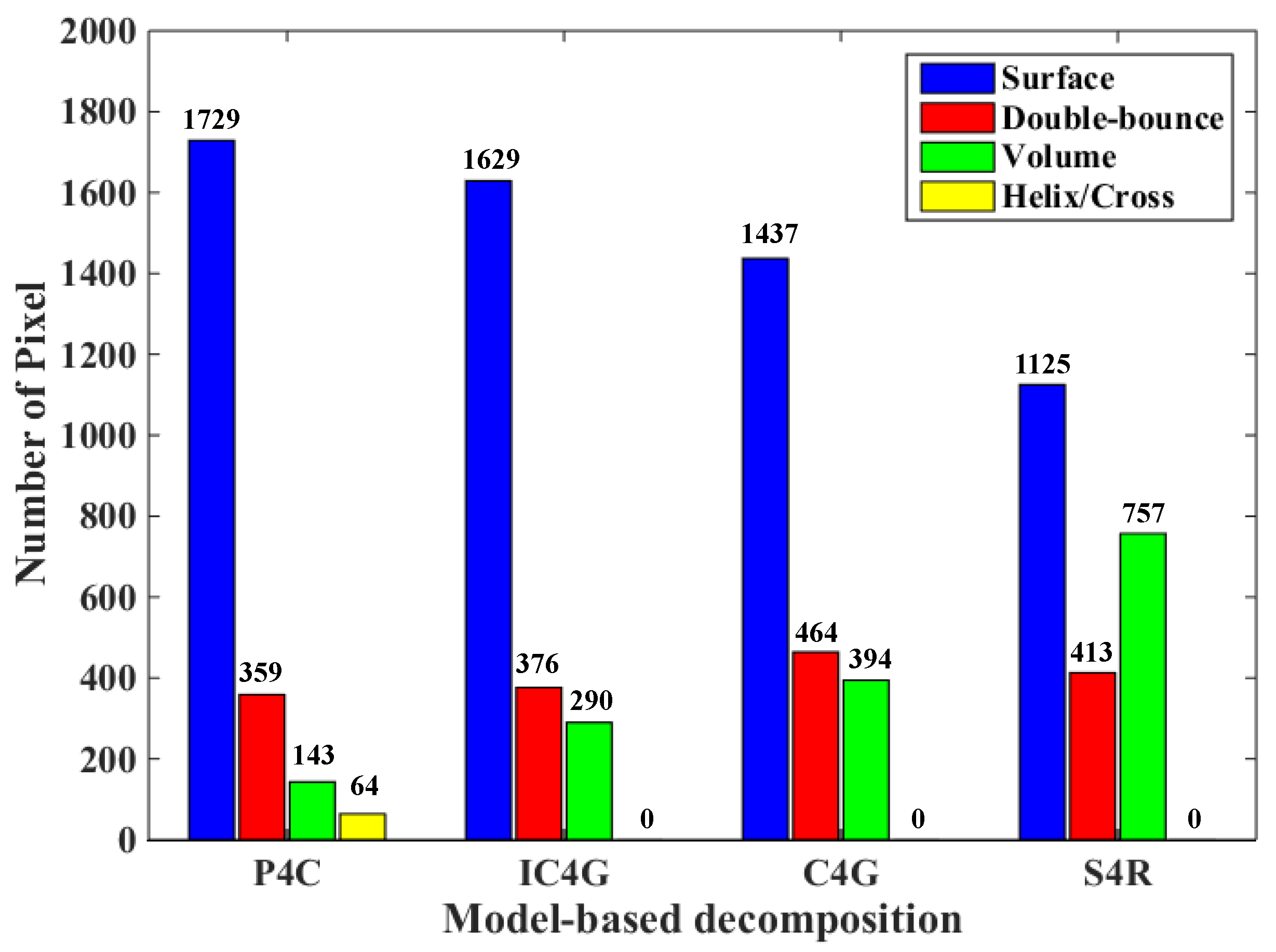
The SMs of ships can also be analyzed from another perspective. The main SM of each pixel is first determined. For a pixel belonging to a ship, after polarimetric decomposition, it has four power components, i.e., $P_s$, $P_d$, $P_v$ and $P_c$ for the proposed method and $P_s$, $P_d$, $P_v$ and $P_h$ for helix matrix-based methods. Referring to Table 1, since the most impacting component (power) is no larger than $50\%$, we regard that the scattering component (power) concurs with the SPANthe most as the main scattering. As an example, if $P_s$ gets the maximum value among the four powers $P_s$, $P_d$, $P_v$ and $P_c$ (or $P_h$), surface scattering is regarded as the main SM of the pixel under test. By this method, we can obtain a main SM pattern for each ship. Figure 5 illustrates a color map of the main SMs of ships in the test area. In this figure, red, green, blue and orange denote double-bounce scattering, volume scattering, surface scattering and cross-polarized (or helix) scattering, respectively. To conveniently observe ship SMs, the sea clutter is colored dark blue. It is seen that the ships exhibit a variety of SMs; no single SM dominates the entire ship. The vast majority of ships are dominated by surface or/and double-bounce scattering, which is an acceptable result. Ships $T_9$, $T_{17}$, $T_{19}$ and $T_{23}$ (refer to the labels in Figure 3) are very likely to have been overestimated by S4R, since almost the whole body of the ship appears green in Figure 5a. This situation is improved by C4G (Figure 5b), except for ship $T_9$, and further improved by IC4G (Figure 5c) and the proposed P4C (Figure 5d). For ships $T_2$, $T_3$, $T_4$, and $T_{10}$, which are dominated by the double-bounce scattering, all methods except for IC4G produce consistent results. Careful observation of Figure 5d indicates that some parts of several ships are dominated by cross-polarized scattering (orange), which indicates that oriented dihedral corners or wires are located in these areas. The main SM distribution for all ship pixels is counted in Figure 6. It shows that the proposed method P4C yields cross-polarized scattering as the main SM for only a small proportion of pixels. As analyzed above, this result is reasonable. In general, surface scattering and double-bounce scattering are the first and second dominant SMs for ships, which is validated by the results of C4G, IC4G and P4C. The volume scattering is overestimated by S4R, causing it to become the second dominant SM.

4.3. Reflection Asymmetry Description

In this experiment, we explored the characteristics of the cross-polarized coherency matrix $\langle {\left[T\right]}_c\rangle$ used in P4C and the helix matrix $\langle {\left[T\right]}_h\rangle$ used in S4R, C4G and IC4G by comparing them with the observed coherency matrix ${\langle \left[T\right]\rangle }^{HV}$. The real measurement of ${\langle \left[T\right]\rangle }^{HV}$ and its corresponding orientation compensation matrix $\langle {\left[T\right]}_r\rangle$, cross-polarized matrix $\langle {\left[T\right]}_c\rangle$ and helix matrix $\langle {\left[T\right]}_h\rangle$ is presented in Equations (21)–(24), respectively.

$$\begin{array}{c}\hfill {\langle \left[T\right]\rangle }^{HV}=\left[\begin{array}{ccc}0.0617& -0.0048-0.0011i& +0.0006-0.0007i\\ -0.0048+0.0011i& 0.0020& -0.0002+0.0002i\\ +0.0006+0.0007i& -0.0002-0.0002i& 0.0007\end{array}\right]\end{array}$$

(21)

$$\begin{array}{c}\hfill \langle {\left[T\right]}_r\rangle =\left[\begin{array}{ccc}0.0617& -0.0048-0.0010i& -0.0002-0.0008i\\ -0.0048+0.0010i& 0.0021& +0.0000+0.0002i\\ -0.0002+0.0008i& +0.0000-0.0002i& 0.0006\end{array}\right]\end{array}$$

(22)

$$\begin{array}{c}\hfill \langle {\left[T\right]}_c\rangle =\left[\begin{array}{ccc}1.1186& -0.1252+0.0221i& 0.4629-0.5106i\\ -0.1252-0.0221i& 0.4211& 0.1232+0.0983i\\ 0.4629+0.5106i& 0.1232-0.0983i& 0.3847\end{array}\right]\end{array}$$

(23)

$$\begin{array}{c}\hfill \langle {\left[T\right]}_h\rangle =\left[\begin{array}{ccc}0& 0& 0\\ 0& 1& \pm i\\ 0& \mp i& 1\end{array}\right]\end{array}$$

(24)

$$\begin{array}{c}\hfill P_h=2|Im\left\{{\langle \left[T\right]\rangle }^{HV}(2,3)\right\}|\end{array}$$

(25a)

$$\begin{array}{c}\hfill P_h=2|Im\left\{\langle {\left[T\right]}_r\rangle (2,3)\right\}|\end{array}$$

(25b)

In Equation (21), one can easily find that the element ${\langle \left[T\right]\rangle }^{HV}(2,3)$ of the observed coherency matrix has a certain complex value. A non-zero ${\langle \left[T\right]\rangle }^{HV}(2,3)$ or $\langle (S_{HH}-S_{VV})S_{HV}^{*}\rangle \ncong 0$ means that the reflection symmetry condition does not hold for the observed targets, and this should be considered in the decomposition method. The element $\langle {\left[T\right]}_c\rangle (2,3)$ of the proposed cross-polarized coherency, as shown in Equation (23), has a non-zero value just like ${\langle \left[T\right]\rangle }^{HV}(2,3)$ does, and this permits us to account for the reflection asymmetry. Furthermore, it is very important to note that the real parts of both ${\langle \left[T\right]\rangle }^{HV}(2,3)$ and $\langle {\left[T\right]}_c\rangle (2,3)$ are non-zero. This characteristic causes the proposed coherency matrix $\langle {\left[T\right]}_c\rangle$ to match the observed coherency matrix ${\langle \left[T\right]\rangle }^{HV}$ (no orientation compensation applied) more accurately than the helix matrix $\langle {\left[T\right]}_h\rangle$, as shown in Equation (24), whose real part is zero. Since the element $\langle {\left[T\right]}_h\rangle (2,3)$ is a pure imaginary number, only the imaginary part of ${\langle \left[T\right]\rangle }^{HV}(2,3)$ is considered when calculating the reflection asymmetry power (Equation (25)). Although the special unitary transformation known as orientation angle compensation can convert ${\langle \left[T\right]\rangle }^{HV}(2,3)$ to a pure imaginary number (Equation (22)) and maintain the total information of ${\langle \left[T\right]\rangle }^{HV}$, helix matrix-based decomposition methods [16,17,21,24] cannot take the reflection asymmetry information contained in the real part of ${\langle \left[T\right]\rangle }^{HV}(2,3)$ into account, resulting in a low estimation of the reflection asymmetry power. In addition, the helix matrix totally misses matching the ${\langle \left[T\right]\rangle }^{HV}(1,3)$ element, which is another term related to reflection asymmetry. As a result, the reflection asymmetry power of ships is underestimated, as can be corroborated from Figure 6, which shows that no ship pixel is dominated by helix scattering in the results of S4R, C4G and IC4G.

4.4. Ship Detection by SM-Based Metrics

Based on the analysis of SMs of ship targets and sea clutter as described in Section 4.2, the dominant SM of sea clutter is surface scattering, while the SMs of ships are relatively complex. Broadly speaking, the dominant SM of ships is also surface scattering, which is consistent with the results obtained by various decomposition methods, as shown in Table 1 and Figure 5. Except for surface scattering, for the proposed method, double-bounce and cross-polarized scattering account for a considerable amount of the total power. This difference in the SM between the sea clutter and the ships allows us to detect the ships using model-based decomposition analysis. In this paper, we propose a novel metric for separating ships from the surrounding sea clutters, which is defined as:

$$\mathbb{M}=ln\frac{P_d+P_c}{P_s}$$

(26)

This metric is proposed based on the following concept: $\mathbb{M}$ will lead to a relatively large value for ship targets compared to that for sea clutter, since the power of double-bounce and cross-polarized scattering is considerably small for sea clutter, while surface scattering is the dominant power. Intuitively, this metric can effectively enhance the signal-to-clutter ratio (SCR) and improve the detection performance. For the purpose of comparison, we use $P_h$, i.e., the counterpart of $P_c$, to construct similar metrics for the other three decomposition methods:

$${\mathbb{M}}^{*}=ln\frac{P_d+P_h}{P_s}$$

(27)

We know that for the other three decomposition methods, if we use $P_v$ instead of $P_h$, better detection performance may be obtained (especially for the method of S4R). However, this is not done because $P_v$ is overestimated and cannot reveal the correct SMs of ships, as discussed in previous sections.

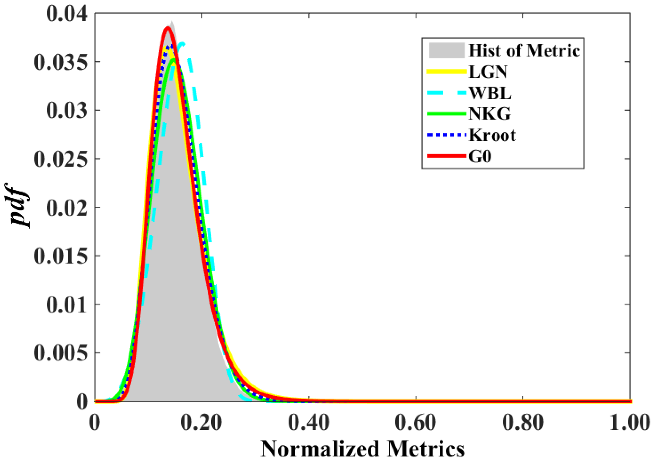
To evaluate the performance of comparative methods, we combine the proposed metric with a classical constant false alarm rate (CFAR) detector [3]. For selecting the optimal probability density function (pdf) to model the sea background for the $\mathbb{M}$ image, we conducted an experiment to evaluate the candidate pdfs, including the lognormal (LGN), the Weibull (WBL), the Nakagami (NKG), the $\mathcal{K}$-root and the ${\mathcal{G}}^0$ distributions. The detailed definitions of these distributions are presented in a comparative study by Cui et al. [28]. The parameters of the models were estimated using the method of log-cumulants (MoLC) [29]. The goodness of fit of the comparative models was measured by the Kullback–Leibler (KL) distance [30], which approximates to zero, indicating that the estimated pdf perfectly fits the actual sea background distribution. The statistical distribution of the sea background, together with the candidate pdf’s for the metrics image, is shown in Figure 7. Among these pdf’s, the ${\mathcal{G}}^0$ distribution (red line) shows the highest similarity to the sea background distribution (grey area). The detailed KL distances for the five distributions are LGN (0.0299), WBL (0.1781), NKG (0.0696), $\mathcal{K}$-root (0.0393) and ${\mathcal{G}}^0$ (0.0218). Thus, in the following experiments, we utilized a ${\mathcal{G}}^0$-CFAR detector to conduct the ship detection task for the test image. The detection threshold was adaptively determined based on modeling the pdf of a local sea background by the ${\mathcal{G}}^0$ distribution (a sliding window method [2,3] was used in our experiment), in combination with a given false alarm probability ($PFA$).

We evaluated the comparative methods and the proposed method quantitatively by utilizing the receiver operating characteristic (ROC) [31], which plots the pixel-level factor of the metric criterion ($FoM$) (in this paper, we use pixel-level FoM, rather than target-level FoM, to evaluate the ship detection performance, since all comparative methods yield FoM values close to one for the latter and cannot reveal the difference between methods) against the false alarm rate ($P_{fa}$), to characterize the overall ship detection performance. The $FoM$ and $P_{fa}$ are defined by:

$$\begin{array}{cc}\hfill FoM& =\frac{TP}{TP+FN+FP}\hfill \\ \hfill P_{fa}& =\frac{FP}{FP+TN}\hfill \end{array}$$

(28)

where $TP$ (true positive) and $TN$ (true negative) denote the number of correctly-detected ship target pixels and sea clutter pixels, respectively. $FP$ (false positive) and $FN$ (false negative) denote the number of false alarm pixels and missing ship target pixels, respectively. $TP+FN$ denotes the actual number of ship target pixels and is commonly referred to as the ground truth, which was marked by the expert interpreter as shown in Figure 3b. It should be noted that the terms $PFA$ and $P_{fa}$ are two different parameters. $PFA$ is a preset parameter representing the expected false alarm rate to calculate the adaptive detection threshold, whereas $P_{fa}$ represents the actual false alarm rate defined by Equation (28).

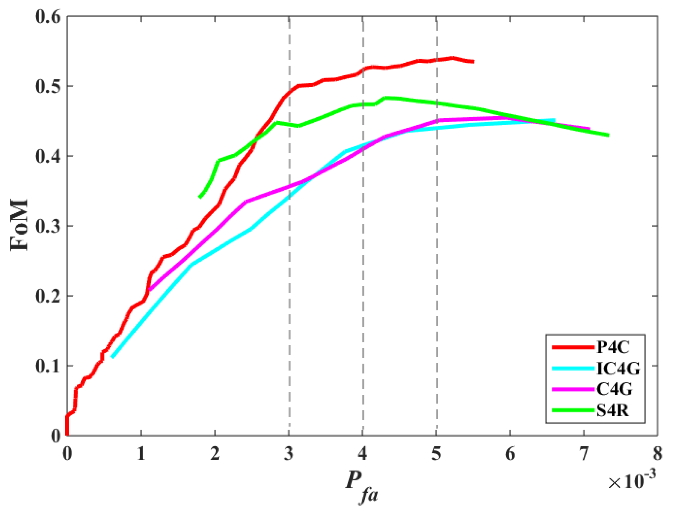
To plot an ROC curve for a comparative method, the experiments were run on the test image with a series of pre-defined $PFA$ values, which were selected successively from a set $PFA=\{1\times {10}^{-6},...,9\times {10}^{-6},...,1\times {10}^{-3},...,9\times {10}^{-3},0.01\}$. For each run with a given $PFA$, the intermediate results $TP$, $TN$, $FN$ and $FP$ were calculated based on the ground truth image, after which the subsequent $FoM$ and $P_{fa}$ were obtained based on Equation (28) and a point generated $(P_{fa},FoM)$ on the curve. After all runs, the $FoM/P_{fa}$ curve for the corresponding method was plotted. The process described above was repeated for all comparative methods, and the final ROC curves are plotted in Figure 8. From this result, we can see that, visually, the curve plotted based on the metrics obtained by the proposed decomposition method P4C is located at the top-left side compared to those obtained by the other methods. This indicates that generally speaking, the performance of the detector based on the proposed metric outperforms the comparative methods.

From another viewpoint, the factor of the metric criterion ($FoM$) of the different detectors was compared in terms of the extent to which this rate corresponded to the same observed false alarm rate $P_{fa}=0.003$, $P_{fa}=0.004$, and $P_{fa}=0.005$, respectively. The details are listed in

Table 2. $FoM$ under specific $P_{fa}$ for comparative methods.

	$\mathit{P}4\mathit{C}$	$\mathit{IC}4\mathit{G}$	$\mathit{C}4\mathit{G}$	$\mathit{S}4\mathit{R}$
$P_{fa}=3\times {10}^{-3}$	0.494	0.343	0.353	0.443
$P_{fa}=4\times {10}^{-3}$	0.525	0.406	0.396	0.474
$P_{fa}=5\times {10}^{-3}$	0.537	0.445	0.451	0.475
Average value	0.519	0.398	0.400	0.464

. It is seen that the detector based on the proposed metric achieved the highest performance. The average value of $FoM$ is $0.519$. The gain to the second best method S4R ($0.464$)) is more than $5\%$ and more than $10\%$ to the methods of IC4G ($0.398$) and C4G ($0.400$). Considering that the $FoM$ is measured at the pixel-level, this is a very encouraging result. Another advantage of the proposed metric is that for the large range of change of the expected $PFA$, the maximum of the real false alarm rate $P_{fa}$ is not more than $6\times {10}^{-3}$, but preserves a high $FoM$, which is close to $0.550$. These results prove that the proposed metric obtained by our four-component model-based polarimetric decomposition method is feasible to be applied for ship detection.

5. Conclusions

For the purpose of presenting a more accurate interpretation of ships’ SMs, a four-component model-based decomposition method is proposed. The proposed method models the SMs of ships with surface, double-bounce, volume and cross-polarized components based on a priori domain knowledge of ships. Some conclusions can be summarized as follows:

(1)

The comprehensive comparative experiments demonstrate that the proposed cross-polarized scattering component can mitigate the overestimation of volume scattering effectively by discriminating the scattering power generated by the oriented scatterers, such as dihedral corners and oriented wires from volume scattering power. This cross-polarized scattering component can also completely describe the reflection asymmetry by accounting for both the real and imaginary parts of the observed coherency matrix to retain the information lost by the existing helix matrix-based methods. This characteristics makes the proposed method capable of presenting a more accurate interpretation of the SMs of ships.

(2)

Based on the proposed decomposition method and an analysis of the difference of SMs between ships and sea clutter, a novel ship detection metric defined as $\mathbb{M}=ln\frac{P_d+P_c}{P_s}$ is proposed. The experiments prove that the proposed ship detection metric can effectively enhance the signal-to-clutter ratio (SCR) and improve the detection performance. The average gain evaluated by pixel-level $FoM$ for the existing methods is more than $5\%$ compared to S4R and even more than $5\%$ compared to IC4G and C4G.

Since different types of ships have different superstructures, and consequently different SMs, it is highly desirable to classify ships based on the correct SM analysis. The proposed four-component model-based decomposition method provides the possibility to understand the SMs of ships more accurately. Because of the limitations in the PolSAR data we now have, we have not yet pursued such a study. In our future work, we will further explore the feasibility of using the decomposed parameters by the proposed method for ship classification.

References

- Brusch, S.; Lehner, S.; Fritz, T.; Soccorsi, M.; Soloviev, A.; van Schie, B. Ship surveillance with TerraSAR-X. IEEE Trans. Geosci. Remote Sens. 2011, 49, 1092–1103. [Google Scholar] [CrossRef]
- Crisp, D.J. The State-of-the-art in Ship Detection in Synthetic Aperture Radar Imagery; Defence Science and Technology Organisation Salisbury (Australia) Info Sciences Lab: Canberra, Astralia, 2004. [Google Scholar]
- El-Darymli, K.; McGuire, P.; Power, D.; Moloney, C. Target detection in synthetic aperture radar imagery: A state-of-the-art survey. J. Appl. Remote Sens. 2013, 7, 071598. [Google Scholar] [CrossRef]
- Stasolla, M.; Mallorquí, J.J.; Margarit, G.; Santamaria, C.; Walker, N. A Comparative Study of Operational Vessel Detectors for Maritime Surveillance Using Satellite-Borne Synthetic Aperture Radar. IEEE J. Sel. Top. Appl. Earth Obs. Remote Sens. 2016, 9, 2687–2701. [Google Scholar] [CrossRef]
- Margarit, G.; Tabasco, A. Ship Classification in Single-Pol SAR Images Based on Fuzzy Logic. IEEE Trans. Geosci. Remote Sens. 2011, 49, 3129–3138. [Google Scholar] [CrossRef]
- Zhang, H.; Tian, X.; Wang, C.; Wu, F.; Zhang, B. Merchant vessel classification based on scattering component analysis for COSMO-SkyMed SAR images. IEEE Geosci. Remote Sens. Lett. 2013, 10, 1275–1279. [Google Scholar] [CrossRef]
- Xing, X.; Ji, K.; Zou, H.; Chen, W.; Sun, J. Ship Classification in TerraSAR-X Images With Feature Space Based Sparse Representation. IEEE Geosci. Remote Sens. Lett. 2013, 10, 1562–1566. [Google Scholar] [CrossRef]
- Lang, H.; Zhang, J.; Zhang, X.; Meng, J. Ship Classification in SAR Image by Joint Feature and Classifier Selection. IEEE Geosci. Remote Sens. Lett. 2016, 13, 212–216. [Google Scholar] [CrossRef]
- Novak, L.M.; Irving, W.W. Optimal Polarimetric Processing for Enhanced Target Detection. IEEE Trans. Aerosp. Electron. Syst. 1993, 29, 234–244. [Google Scholar] [CrossRef]
- Chen, J.; Chen, Y.; Yang, J. Ship detection using polarization cross-entropy. IEEE Geosci. Remote Sens. Lett. 2009, 6, 723–727. [Google Scholar] [CrossRef]
- Wang, N.; Shi, G.; Liu, L.; Zhao, L.; Kuang, G. Polarimetric SAR target detection using the reflection symmetry. IEEE Geosci. Remote Sens. Lett. 2012, 9, 1104–1108. [Google Scholar] [CrossRef]
- Marino, A. A notch filter for ship detection with polarimetric SAR data. IEEE J. Sel. Top. Appl. Earth Obs. Remote Sens. 2013, 6, 1219–1232. [Google Scholar] [CrossRef]
- Wang, J.; Huang, W.; Yang, J.; Chen, P.; Zhang, H. Polarization scattering characteristics of some ships using polarimetric SAR images. In Proceedings of the SPIE Remote Sensing. International Society for Optics and Photonics, Prague, Czech Republic, 19 September 2011; p. 81790W. [Google Scholar]
- Freeman, A.; Durden, S.L. A three-component scattering model for polarimetric SAR data. IEEE Trans. Geosci. Remote Sens. 1998, 36, 963–973. [Google Scholar] [CrossRef]
- Sugimoto, M.; Ouchi, K.; Nakamura, Y. On the novel use of model-based decomposition in SAR polarimetry for target detection on the sea. Remote Sens. Lett. 2013, 4, 843–852. [Google Scholar] [CrossRef]
- Yamaguchi, Y.; Sato, A.; Boerner, W.M.; Sato, R.; Yamada, H. Four-component scattering power decomposition with rotation of coherency matrix. IEEE Trans. Geosci. Remote Sens. 2011, 49, 2251–2258. [Google Scholar] [CrossRef]
- Yamaguchi, Y.; Moriyama, T.; Ishido, M.; Yamada, H. Four-component scattering model for polarimetric SAR image decomposition. IEEE Trans. Geosci. Remote Sens. 2005, 43, 1699–1706. [Google Scholar] [CrossRef]
- Moriyama, T.; Uratsuka, S.; Umehara, T.; Maeno, H. Polarimetric SAR image analysis using model fit for urban structures. IEICE Trans. Commun. 2005, 88, 1234–1243. [Google Scholar] [CrossRef]
- Chen, S.W.; Ohki, M.; Shimada, M.; Sato, M. Deorientation effect investigation for model-based decomposition over oriented built-up areas. IEEE Geosci. Remote Sens. Lett. 2013, 10, 273–277. [Google Scholar] [CrossRef]
- Chen, S.W.; Li, Y.Z.; Wang, X.S.; Xiao, S.P.; Sato, M. Modeling and interpretation of scattering mechanisms in polarimetric synthetic aperture radar: Advances and perspectives. IEEE Signal Process. Mag. 2014, 31, 79–89. [Google Scholar] [CrossRef]
- Sato, A.; Yamaguchi, Y.; Singh, G.; Park, S.E. Four-component scattering power decomposition with extended volume scattering model. IEEE Geosci. Remote Sens. Lett. 2012, 9, 166–170. [Google Scholar] [CrossRef]
- Chen, S.W.; Wang, X.S.; Li, Y.Z.; Sato, M. Adaptive model-based polarimetric decomposition using PolInSAR coherence. IEEE Trans. Geosci. Remote Sens. 2014, 52, 1705–1718. [Google Scholar] [CrossRef]
- Xiang, D.; Ban, Y.; Su, Y. Model-Based Decomposition With Cross Scattering for Polarimetric SAR Urban Areas. IEEE Geosci. Remote Sens. Lett. 2015, 12, 2496–2500. [Google Scholar] [CrossRef]
- Chen, S.W.; Wang, X.S.; Xiao, S.P.; Sato, M. General polarimetric model-based decomposition for coherency matrix. IEEE Trans. Geosci. Remote Sens. 2014, 52, 1843–1855. [Google Scholar] [CrossRef]
- An, W.; Cui, Y.; Yang, J. Three-component model-based decomposition for polarimetric SAR data. IEEE Trans. Geosci. Remote Sens. 2010, 48, 2732–2739. [Google Scholar]
- Yamaguchi, Y.; Yajima, Y.; Yamada, H. A four-component decomposition of POLSAR images based on the coherency matrix. IEEE Geosci. Remote Sens. Lett. 2006, 3, 292–296. [Google Scholar] [CrossRef]
- Nunziata, F.; Migliaccio, M.; Brown, C.E. Reflection symmetry for polarimetric observation of man-made metallic targets at sea. IEEE J. Ocean. Eng. 2012, 37, 384–394. [Google Scholar] [CrossRef]
- Cui, S.; Schwarz, G.; Datcu, M. A Comparative Study of Statistical Models for Multilook SAR Images. IEEE Geosci. Remote Sens. Lett. 2014, 11, 1752–1756. [Google Scholar]
- Krylov, V.A.; Moser, G.; Serpico, S.B.; Zerubia, J. On the method of logarithmic cumulants for parametric probability density function estimation. IEEE Trans. Image Process. 2013, 22, 3791–3806. [Google Scholar] [CrossRef] [PubMed]
- Kullback, S. Letter to the editor: The Kullback-Leibler distance. Am. Stat. 1987, 41, 340–341. [Google Scholar]
- Fawcett, T. An introduction to ROC analysis. Pattern Recognit. Lett. 2006, 27, 861–874. [Google Scholar] [CrossRef]
Figure 1.
Scattering mechanism analysis of ships at sea. : total backscattered power. : surface scattering power. : double-bounce scattering power. : volume scattering power. : cross-polarized scattering power.
Figure 2.
Flowchart of the four-component decomposition algorithm. The total power of these four components equals .
Figure 3.
(a) PolSAR data of Hong Kong area. The blue rectangle marks the sampling area in the experiments. (b) The ground truth of the location and contour of the ship in the sampling area.
Figure 4.
Combined RGB images of different decomposition results of (a) , (b) , (c) and (d) , respectively (red: , green: , blue: ).
Figure 5.
Ships’ main scattering mechanisms (SMs) of different decompositions. (a) The decomposition results of S4R, (b) C4G, (c) IC4G and (d) P4C. Only ships’ main SMs are calculated and colored in: red: , green: , blue: , yellow: (). Sea area is the dominant surface, but is colored dark blue to facilitate convenient observation of ship SMs.
Figure 6.
Distributions of main SMs for different scattering models. The total number of ship pixels is 2295.
Figure 7.
The pre-selection of the sea clutter modeling method for the metrics image.
Figure 8.
Ship detection performance evaluation on the factor of the metric criterion (FoM) for different decomposition methods.