
Estimation of Surface NO2 Volume Mixing Ratio in Four Metropolitan Cities in Korea Using Multiple Regression Models with OMI and AIRS Data


Abstract
:
1. Introduction
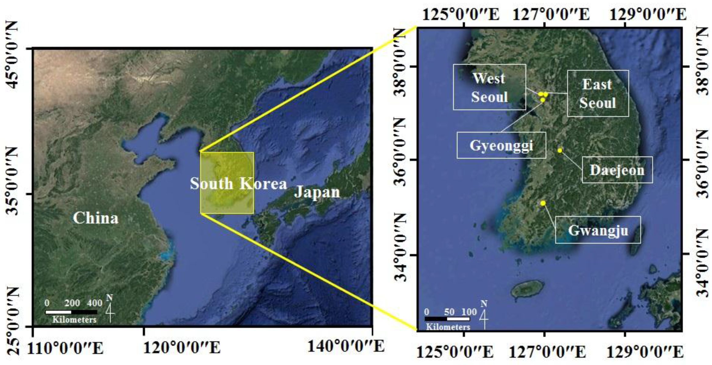
2. Study Area and Period
2.1. Data
2.1.1. Ozone Monitoring Instrument (OMI) Data
2.1.2. Atmospheric Infrared Sounder (AIRS) Data
2.1.3. In Situ NO2 Data
2.1.4. In Situ Meteorological Data
3. Methodology
3.1. M1
3.2. M2
3.3. M3 and M4
4. Results
4.1. Daily Estimates
4.2. Monthly Estimates
5. Discussion
5.1. Estimation of Surface NO2 VMRs at a Specific Time (13:45 LT)
- Among the three regression models, the multiple regression model M3 performed best in estimating NO2 VMRST. The linear regression model (M2), in which BLH is used as an independent variable in addition to Trop NO2 VCDOMI, has comparable performance to that of the model (M1) which uses Trop NO2 VCDOMI as the only independent variable.The BLH varies with latitude [36], but the latitudinal variation of BLH is not well represented since the spatial resolution of the AIRS used in this study is coarser than the spatial resolution of OMI. It might also be associate the BLHAIRS data quality. We expect better results using BLH data obtained from LIDAR.
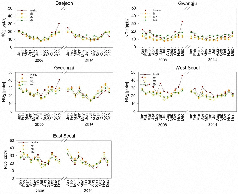
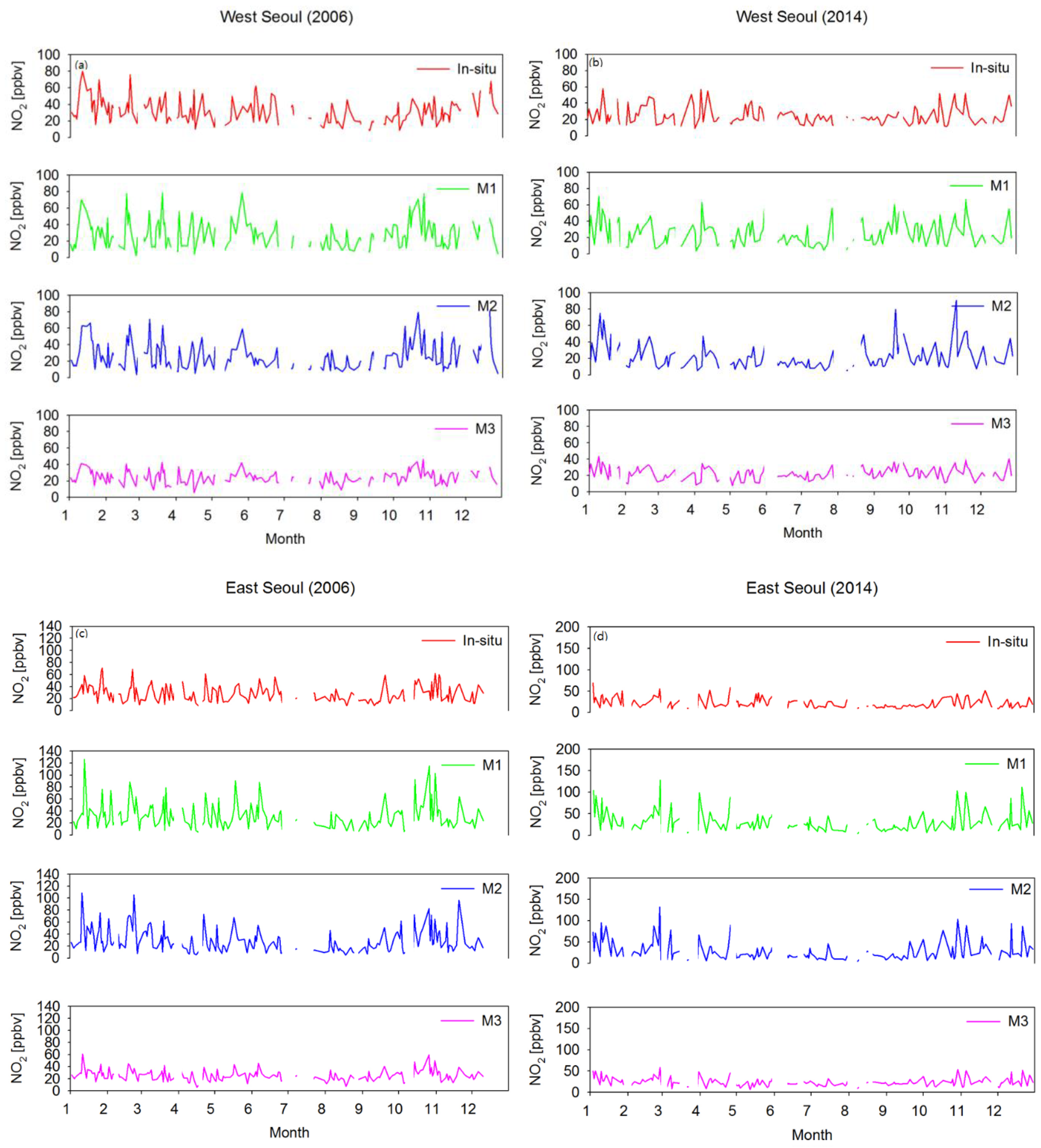
- The average difference was found to be 46.04% between NO2 VMRIn-situ and NO2 VMRST obtained from M1, 44.29% between NO2 VMRIn-situ and NO2 VMRST obtained from M2, and 31.50% between NO2 VMRIn-situ and NO2 VMRST obtained from M3 in all cities, while there was moderate agreement in the temporal pattern of NO2 variation between NO2 VMRIn-situ and NO2 VMRST obtained from M1, M2, and M3 (Figure 6).
- In terms of statistical evaluation with respect to the in situ data, M3 showed the best performance in general.
- The results produced by M2 are not improved compared to those by M1 which may imply that surface NO2 VMR is dominantly affected by tropospheric NO2 column while the BLH effect could be negligible in areas of the present study. It might also be associate the AIRS BLH data quality.
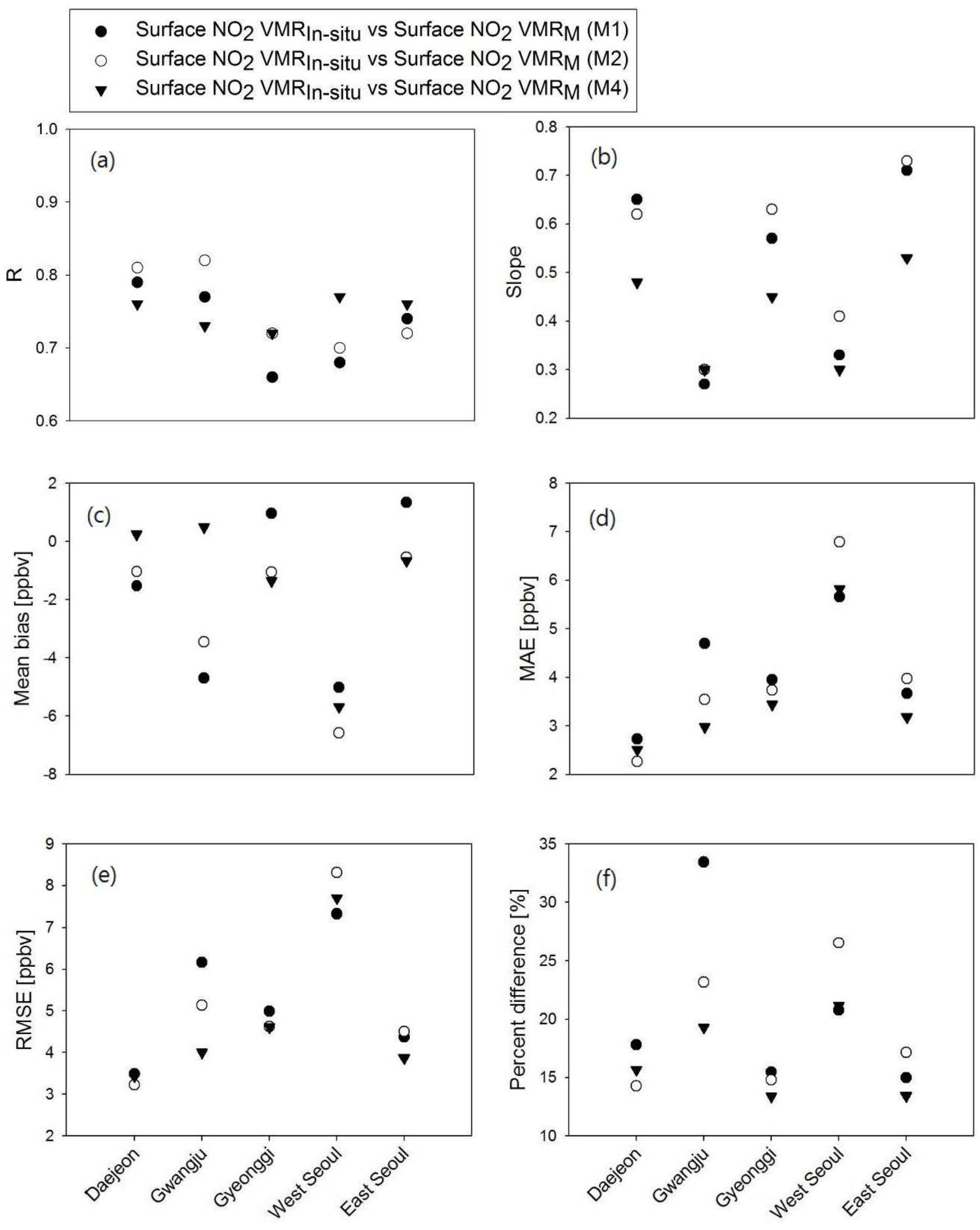
5.2. Estimation of Monthly Mean Surface NO2 VMRs of a Specific Time (13:45 LT)
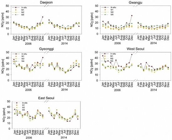
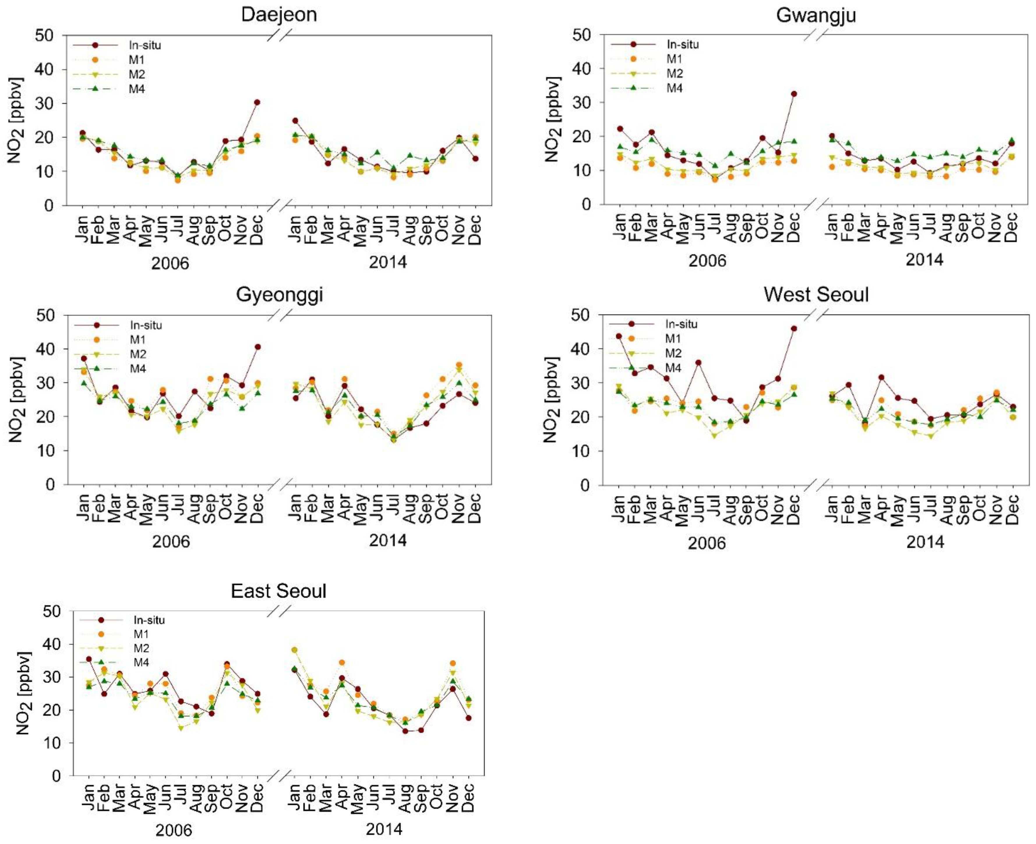
- We found good agreement in the temporal pattern between the estimated NO2 VMRM and monthly mean NO2 VMRIn-situ (Figure 8). However, there was a large difference between NO2 VMRIn-situ and NO2 VMRM in the period when there was a clear change in NO2 VMRM between one month and the next. Despite the use of NO2 VMRIn-situ located away from streets, the in situ measurement sites in West Seoul are located closer to streets than the in situ measurement sites in Daejeon and Gwangju. This may explain why there are more periods when NO2 VMRIn-situ changes rapidly in successive months. It is difficult to estimate the rapid change of NO2 VMR near NO2 sources with regression models that reflect the relationship between the in situ measurements and the OMI sensor covering both source and non-source areas in a single pixel.
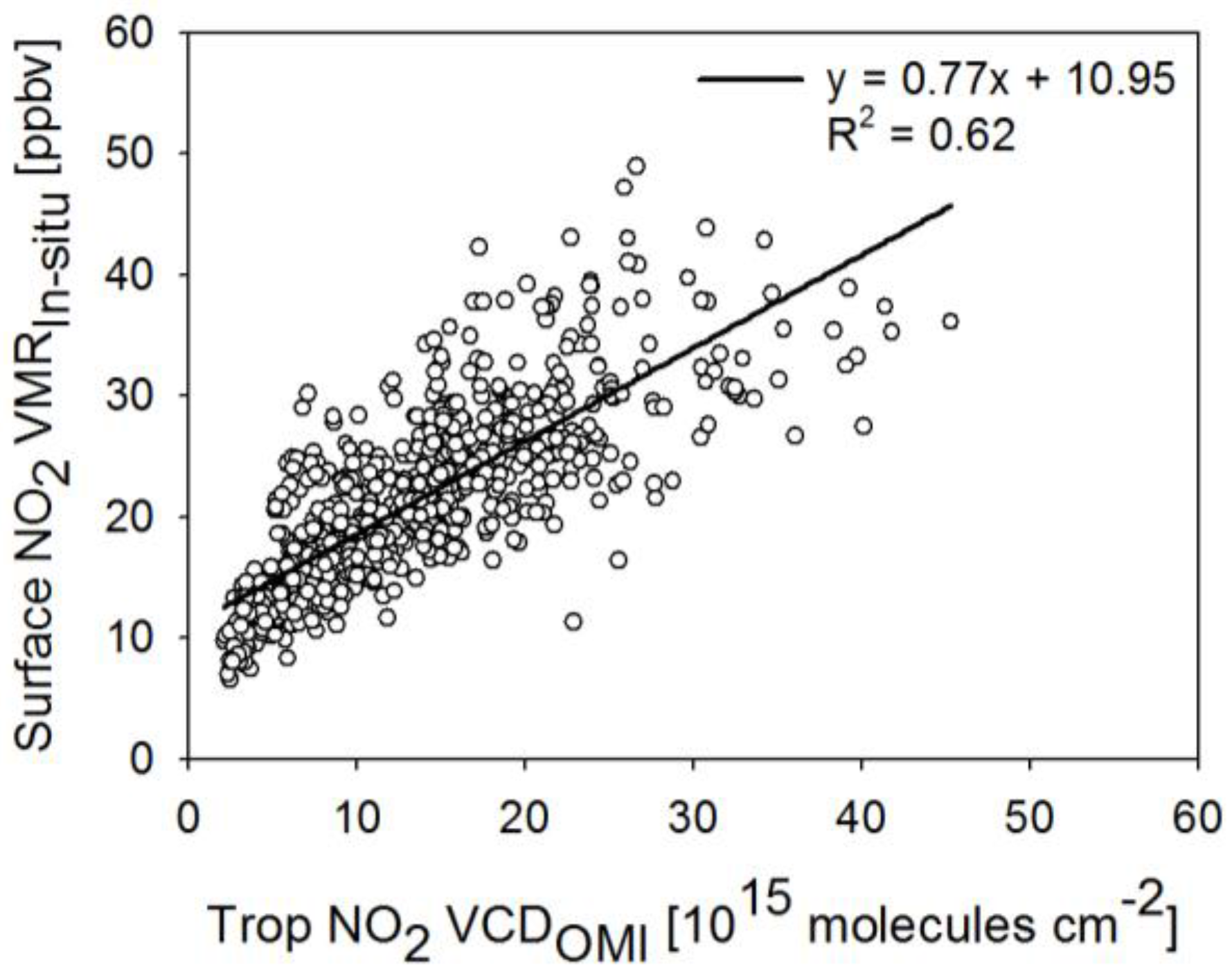
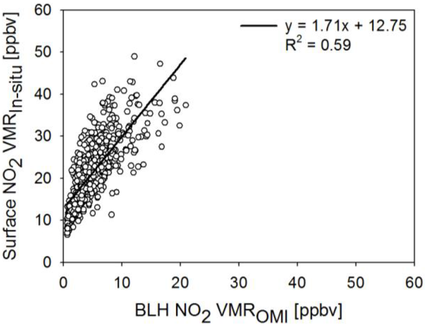
- In terms of statistical evaluation, the three regression models (M1, M2, and M4) were found to be similar (Figure 9).
- NO2 VMRM shows better agreement with the NO2 VMRIn-situ than does NO2 VMRST. The reason for the better performance in the monthly mean estimation could be attributed to reduced errors in the monthly mean OMI data [37] as well as fewer occasions with sudden monthly changes in NO2 VMRIn-situ than rapid day-to-day changes in NO2 VMRIn-situ.
6. Conclusions
Supplementary Materials
Acknowledgments
Author Contributions
Conflicts of Interest
References
- IPCC. Climate Change 2007: The Physical Science Basis. In Contribution of Working Group I to the Fourth Assessment Report of the Intergovernmental Panel on Climate Change; Solomon, S., Qin, D., Manning, M., Chen, Z., Marquis, M., Averyt, K.B., Tignor, M., Miller, H.L., Eds.; Cambridge University Press: Cambridge, UK; New York, NY, USA, 2007; p. 2007. [Google Scholar]
- Van der A, R.J.; Eskes, H.J.; Boersma, K.F.; Van Noije, T.P.C.; Van Roozendael, M.; De Smedt, I.; Peters, D.H.M.U.; Meijer, E.W. Trends, seasonal variability and dominant NOx source derived from a ten year record of NO2 measured from space. J. Geophys. Res. Atmos. 2008, 113. [Google Scholar] [CrossRef]
- Kharol, S.K.; Martin, R.V.; Philip, S.; Boys, B.; Lamsal, L.N.; Jerrett, M.; Brauer, M.; Crouse, D.L.; McLinden, C.; Burnett, R.T.; et al. Assessment of the magnitude and recent trends in satellite-derived ground-level nitrogen dioxide over North America. Atmos. Environ. 2015, 118, 236–245. [Google Scholar]
- Ackermann-Liebrich, U.; Leuenberger, P.; Schwartz, J.; Schindler, C.; Monn, C.; Bolognini, G.; Bongard, J.P.; Brändli, O.; Domenighetti, G.; Elsasser, S.; et al. Lung function and long term exposure to air pollutants in Switzerland. Study on Air Pollution and Lung Diseases in Adults (SAPALDIA) Team. Am. J. Respir. Crit. Care Med. 1997, 155, 122–129. [Google Scholar] [PubMed]
- Schindler, C.; Ackermann-Liebrich, U.; Leuenberger, P.; Monn, C.; Rapp, R.; Bolognini, G.; Bongard, J.P.; Brändli, O.; Domenighetti, G.; Karrer, W.; et al. Associations between Lung Function and Estimated Average Exposure to NO2 in Eight Areas of Switzerland. Epidemiology 1998, 9, 405–411. [Google Scholar] [CrossRef] [PubMed]
- James Gauderman, W.; McConnell, R.O.B.; Gilliland, F.; London, S.; Thomas, D.; Avol, E.; Vora, H.; Berhane, K.; Rappaport, E.B.; Lurmann, F.; et al. Association between air pollution and lung function growth in southern California children. Am. J. Respir. Crit. Care Med. 2000, 162, 1383–1390. [Google Scholar] [CrossRef] [PubMed]
- Panella, M.; Tommasini, V.; Binotti, M.; Palin, L.; Bona, G. Monitoring nitrogen dioxide and its effects on asthmatic patients: Two different strategies compared. Environ. Monit. Assess. 2000, 63, 447–458. [Google Scholar]
- Smith, B.J.; Nitschke, M.; Pilotto, L.S.; Ruffin, R.E.; Pisaniello, D.L.; Willson, K.J. Health effects of daily indoor nitrogen dioxide exposure in people with asthma. Eur. Respir. J. 2000, 16, 879–885. [Google Scholar] [PubMed]
- Boersma, K.F.; Jacob, D.J.; Trainic, M.; Rudich, Y.; DeSmedt, I.; Dirksen, R.; Eskes, H.J. Validation of urban NO2 concentrations and their diurnal and seasonal variations observed from the SCIAMACHY and OMI sensors using in situ surface measurements in Israeli cities. Atmos. Chem. Phys. 2009, 9, 3867–3879. [Google Scholar] [CrossRef]
- Demerjian, K.L. A review of national monitoring networks in North America. Atmos. Environ. 2000, 34, 1861–1884. [Google Scholar] [CrossRef]
- Bechle, M.J.; Millet, D.B.; Marshall, J.D. Remote sensing of exposure to NO2: Satellite versus ground-based measurement in a large urban area. Atmos. Environ. 2013, 69, 345–353. [Google Scholar]
- Leue, C.; Wenig, M.; Wagner, T.; Klimm, O.; Platt, U.; Jähne, B. Quantitative analysis of NOx emissions from Global Ozone Monitoring Experiment satellite image sequences. J. Eophys. Res. Atmos. 2001, 106, 5493–5505. [Google Scholar] [CrossRef]
- Richter, A.; Burrows, J.P. Tropospheric NO2 from GOME measurements. Adv. Space Res. 2002, 29, 1673–1683. [Google Scholar] [CrossRef]
- Martin, R.V.; Chance, K.; Jacob, D.J.; Kurosu, T.P.; Spurr, R.J.; Bucsela, E.; Gleason, J.F.; Palmer, P.I.; Bey, I.; Fiore, A.M.; et al. An improved retrieval of tropospheric nitrogen dioxide from GOME. J. Geophys. Res. Atmos. 2002, 107. [Google Scholar] [CrossRef]
- Boersma, K.F.; Eskes, H.J.; Brinksma, E.J. Error analysis for tropospheric NO2 retrieval from space. J. Geophys. Res. Atmos. 2002, 109. [Google Scholar] [CrossRef]
- Boersma, K.F.; Eskes, H.J.; Veefkind, J.P.; Brinksma, E.J.; Van Der A, R.J.; Sneep, M.; Van Der Oord, G.H.J.; Levelt, P.F.; Stammes, P.; Gleason, J.F.; et al. Near-real time retrieval of tropospheric NO2 from OMI. Atmos. Chem. Phys. Discuss. 2006, 6, 12301–12345. [Google Scholar] [CrossRef]
- Bucsela, E.J.; Celarier, E.A.; Wenig, M.O.; Gleason, J.F.; Veefkind, J.P.; Boersma, K.F.; Brinksma, E.J. Algorithm for NO2 vertical column retrieval from the Ozone Monitoring Instrument. IEEE Trans. Geosci. Remote Sens. 2006, 44, 1245–1258. [Google Scholar] [CrossRef]
- Ordónez, C.; Richter, A.; Steinbacher, M.; Zellweger, C.; Nüß, H.; Burrows, J.P.; Prévôt, A.S.H. Comparison of 7 years of satellite-borne and ground-based tropospheric NO2 measurements around Milan, Italy. J. Geophys. Res. Atmos. 2006, 111. [Google Scholar] [CrossRef]
- Kim, N.K.; Kim, Y.P.; Morino, Y.; Kurokawa, J.I.; Ohara, T. Verification of NOx emission inventory over South Korea using sectoral activity data and satellite observation of NO2 vertical column densities. Atmos. Environ. 2013, 77, 496–508. [Google Scholar] [CrossRef]
- Studies–Seoul, M.A.P. NIER. Available online: https://espo.nasa.gov/home/sites/default/files/documents/MAPS-Seoul_White%20Paper_26%20Feb%202015_Final.pdf (accessed on 17 June 2017).
- Levelt, P.F.; Noordhoek, R. OMI Algorithm Theoretical Basis Document Volume I: OMI Instrument, Level 0–1b Processor, Calibration & Operations; ATBD-OMI-01; Version 1.1; NASA: Washington, DC, USA, 2002. Available online: http://www.sciamachy-validation.org/omi/documents/data/OMI_ATBD_Volume_1_V1d1.pdf (accessed on 17 June 2017).
- Celarier, E.A.; Brinksma, E.J.; Gleason, J.F.; Veefkind, J.P.; Cede, A.; Herman, J.R.; Ionov, D.; Goutail, F.; Pommereau, J.P.; Lambert, J.C.; et al. Validation of Ozone Monitoring Instrument nitrogen dioxide columns. J. Geophys. Res. Atmos. 2008, 113. [Google Scholar] [CrossRef]
- Levelt, P.F.; Hilsenrath, E.; Leppelmeier, G.W.; van den Oord, G.H.; Bhartia, P.K.; Tamminen, J.; de Haan, J.F.; Veefkind, J.P. Science objectives of the ozone monitoring instrument. IEEE Trans. Geosci. Remote Sens. 2006, 44, 1199–1208. [Google Scholar] [CrossRef]
- Aumann, H.; Gaiser, S.; Ting, D.; Manning, E. AIRS Algorithm Theoretical Basis Document Level 1B Part 1: Infrared Spectrometer; EOS Project Science Office, NASA Goddard Space Flight Center: Greenbelt, MD, USA, 1999.
- Fetzer, E.; McMillin, L.M.; Tobin, D.; Aumann, H.H.; Gunson, M.R.; McMillan, W.W.; Hagan, D.E.; Hofstadter, M.D.; Yoe, J.; Whiteman, D.N.; et al. Airs/amsu/hsb validation. IEEE Trans. Geosci. Remote Sens. 2003, 41, 418–431. [Google Scholar] [CrossRef]
- Aumann, H.H.; Chahine, M.T.; Gautier, C.; Goldberg, M.D.; Kalnay, E.; McMillin, L.M.; Revercomb, H.; Rosenkranz, P.W.; Smith, W.L.; Staelin, D.H.; et al. AIRS/AMSU/HSB on the Aqua mission: Design, science objectives, data products, and processing systems. IEEE Trans. Geosci. Remote Sens. 2003, 41, 253–264. [Google Scholar] [CrossRef]
- Chahine, M.T.; Pagano, T.S.; Aumann, H.H.; Atlas, R.; Barnet, C.; Blaisdell, J.; Chen, L.; Divakarla, M.; Fetzer, E.J.; Goldberg, M.; et al. AIRS: Improving Weather Forecasting and Providing New Data on Greenhouse Gases. Bull. Am. Meteorol. Soc. 2006, 87, 911–926. [Google Scholar] [CrossRef]
- Lee, C.J.; Brook, J.R.; Evans, G.J.; Martin, R.V.; Mihele, C. Novel application of satellite and in-situ measurements to map surface-level NO2 in the Great Lakes region. Atmos. Chem. Phys. 2011, 11, 11761–11775. [Google Scholar] [CrossRef]
- Knepp, T.; Pippin, M.; Crawford, J.; Chen, G.; Szykman, J.; Long, R.; Cowen, L.; Cede, A.; Abuhassan, N.; Herman, J.; et al. Estimating surface NO2 and SO2 mixing ratios from fast-response total column observations and potential application to geostationary missions. J. Atmos. Chem. 2015, 72, 261–286. [Google Scholar] [CrossRef] [PubMed]
- Xue, D.; Yin, J. Meteorological influence on predicting surface SO2 concentration from satellite remote sensing in Shanghai, China. Environ. Monit. Assess. 2014, 186, 2895–2906. [Google Scholar] [CrossRef] [PubMed]
- Seidel, D.J.; Ao, C.O.; Li, K. Estimating climatological planetary boundary layer heights from radiosonde observations: Comparison of methods and uncertainty analysis. J. Geophys. Res. Atmos. 2010, 115. [Google Scholar] [CrossRef]
- Cui, W.; Yan, X. Adaptive weighted least square support vector machine regression integrated with outlier detection and its application in QSAR. Chemom. Intell. Lab. Syst. 2009, 98, 130–135. [Google Scholar] [CrossRef]
- Kutner, M.H.; Nachtsheim, C.; Neter, J. Applied linear Regression Models; McGraw-Hill/Irwin: New York, NY, USA, 2004. [Google Scholar]
- Sellke, T.; Bayarri, M.J.; Berger, J.O. Calibration of ρ values for testing precise null hypotheses. Am. Stat. 2001, 55, 62–71. [Google Scholar] [CrossRef]
- Lamsal, L.N.; Martin, R.V.; Van Donkelaar, A.; Steinbacher, M.; Celarier, E.A.; Bucsela, E.; Dunlea, E.J.; Pinto, J.P. Ground-level nitrogen dioxide concentrations inferred from the satellite-borne Ozone Monitoring Instrument. J. Geophys. Res. Atmos. 2008, 113. [Google Scholar] [CrossRef]
- Zeng, X.; Brunke, M.A.; Zhou, M.; Fairall, C.; Bond, N.A.; Lenschow, D.H. Marine atmospheric boundary layer height over the eastern Pacific: Data analysis and model evaluation. J. Clim. 2004, 17, 4159–4170. [Google Scholar] [CrossRef]
- Team, O.M.I. Ozone Monitoring Instrument (OMI) Data User’s Guide; NASA: Washington, DC, USA, 2009; Volume 7, pp. 6–10.


| Data | Time (LT) | ||
|---|---|---|---|
| Satellite | Trop NO2 VCD | OMI Level3 NO2 Daily data (OMNO2d) | 13:45 |
| BLH, Temperature, Pressure | AIRS/Aqua L3 Daily Support Product (AIRS + AMSU) V006 (AIRX3SPD) | 13:30 | |
| In situ | Surface NO2 VMR | Air Korea | 13:00 and 14:00 |
| Surface Temperature, Surface Pressure, Surface Dew point, Surface Wind Speed, Surface Wind Data | AWS (Automatic Weather System) |
| Model | Equation | |
|---|---|---|
| M1 | 13:45 LT and Monthly | |
| M2 | 13:45 LT and Monthly | |
| M3 | 13:45 LT | Section 3, Multiple regression Equation (1) |
| M4 | Monthly | |
| Equation | R2 | ||
|---|---|---|---|
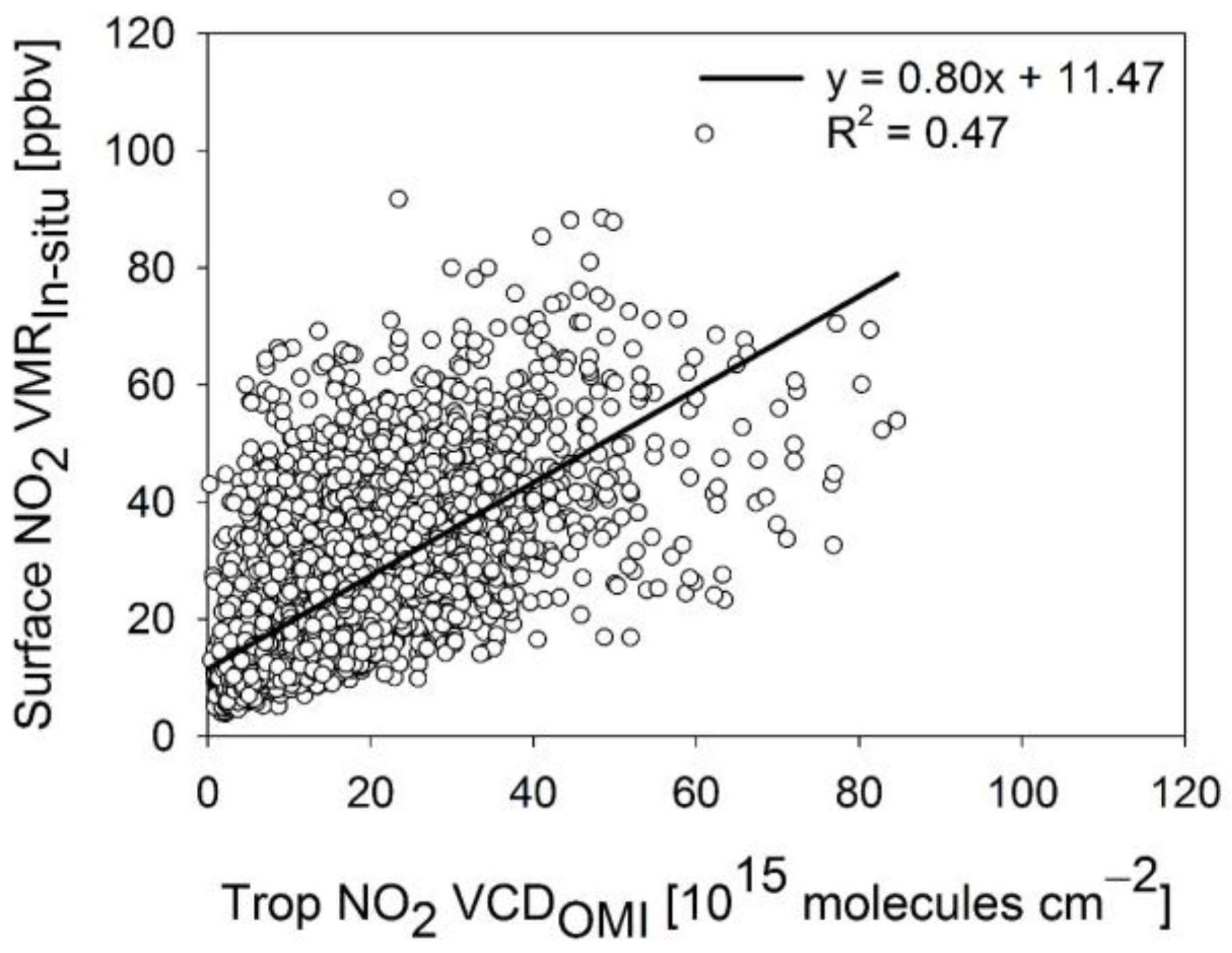
| 13:45 LT | M1 | 0.47 | |
| M2 | 0.38 | ||
| M3 | 0.47 |
| Equation | R2 | ||
|---|---|---|---|
| Monthly mean | M1 | 0.62 | |
| M2 | 0.59 | ||
| M4 | 0.63 |
| Final Selected Independent Variables | p-Value | VIF | |
|---|---|---|---|
| M3 | Trop NO2 VCDOMI | 0 | 1.26 |
| TempIn-situ | 0.000032 | 7.02 | |
| DewpointIn-situ | 0.000306 | 7.16 | |
| PressIn-situ | 0.009981 | 3.14 | |
| BLHAIRS | 1.73 10−15 | 1.12 | |
| WSIn-situ | 3.86 10−133 | 1.33 | |
| WDIn-situ | 1.7493 10−38 | 1.07 | |
| M4 | Trop NO2 VCDOMI | 2.4832 10−89 | 1.64 |
| DewpointIn-situ | 0.000421 | 6.47 | |
| PressIn-situ | 0.034582 | 6.65 | |
| BLHAIRS | 0.000834 | 2.32 | |
| WSIn-situ | 3.86 10−133 | 1.59 | |
| WDIn-situ | 1.699 10−7 | 1.25 |
© 2017 by the authors. Licensee MDPI, Basel, Switzerland. This article is an open access article distributed under the terms and conditions of the Creative Commons Attribution (CC BY) license (http://creativecommons.org/licenses/by/4.0/).
Share and Cite
Kim, D.; Lee, H.; Hong, H.; Choi, W.; Lee, Y.G.; Park, J. Estimation of Surface NO2 Volume Mixing Ratio in Four Metropolitan Cities in Korea Using Multiple Regression Models with OMI and AIRS Data. Remote Sens. 2017, 9, 627. https://0-doi-org.brum.beds.ac.uk/10.3390/rs9060627
Kim D, Lee H, Hong H, Choi W, Lee YG, Park J. Estimation of Surface NO2 Volume Mixing Ratio in Four Metropolitan Cities in Korea Using Multiple Regression Models with OMI and AIRS Data. Remote Sensing. 2017; 9(6):627. https://0-doi-org.brum.beds.ac.uk/10.3390/rs9060627
Chicago/Turabian StyleKim, Daewon, Hanlim Lee, Hyunkee Hong, Wonei Choi, Yun Gon Lee, and Junsung Park. 2017. "Estimation of Surface NO2 Volume Mixing Ratio in Four Metropolitan Cities in Korea Using Multiple Regression Models with OMI and AIRS Data" Remote Sensing 9, no. 6: 627. https://0-doi-org.brum.beds.ac.uk/10.3390/rs9060627