
On the Design of Radar Corner Reflectors for Deformation Monitoring in Multi-Frequency InSAR


Geodesy and Seismic Monitoring Branch, Geoscience Australia, GPO Box 378, Canberra ACT 2601, Australia
Remote Sens. 2017, 9(7), 648; https://0-doi-org.brum.beds.ac.uk/10.3390/rs9070648
Submission received: 19 April 2017
/
Revised: 15 June 2017
/
Accepted: 21 June 2017
/
Published: 25 June 2017
(This article belongs to the Special Issue Advances in SAR: Sensors, Methodologies, and Applications)
Abstract
:Trihedral corner reflectors are being increasingly used as point targets in deformation monitoring studies using interferometric synthetic aperture radar (InSAR) techniques. The frequency and size dependence of the corner reflector Radar Cross Section (RCS) means that no single design can perform equally in all the possible imaging modes and radar frequencies available on the currently orbiting Synthetic Aperture Radar (SAR) satellites. Therefore, either a corner reflector design tailored to a specific data type or a compromise design for multiple data types is required. In this paper, I outline the practical and theoretical considerations that need to be made when designing appropriate radar targets, with a focus on supporting multi-frequency SAR data. These considerations are tested by performing field experiments on targets of different size using SAR images from TerraSAR-X, COSMO-SkyMed and RADARSAT-2. Phase noise behaviour in SAR images can be estimated by measuring the Signal-to-Clutter ratio (SCR) in individual SAR images. The measured SCR of a point target is dependent on its RCS performance and the influence of clutter near to the deployed target. The SCR is used as a metric to estimate the expected InSAR displacement error incurred by the design of each target and to validate these observations against theoretical expectations. I find that triangular trihedral corner reflectors as small as 1 m in dimension can achieve a displacement error magnitude of a tenth of a millimetre or less in medium-resolution X-band data. Much larger corner reflectors (2.5 m or greater) are required to achieve the same displacement error magnitude in medium-resolution C-band data. Compromise designs should aim to satisfy the requirements of the lowest SAR frequency to be used, providing that these targets will not saturate the sensor of the highest frequency to be used. Finally, accurate boresight alignment of the corner reflector can be critical to the overall target performance. Alignment accuracies better than 4° in azimuth and elevation will incur a minimal impact on the displacement error in X and C-band data.
1. Introduction
The Persistent Scatterer Interferometric Synthetic Aperture Radar (PSInSAR) technique [1,2,3,4,5] has become a popular remote sensing method for monitoring ground or infrastructure displacements induced by wide-ranging natural and anthropogenic phenomena. The technique uses a stack of SAR interferograms and determines the motion history for pixels that are identified to have temporal phase stability (i.e., pixels whose overall response is dominated by a strong back-scatterer). The distribution of these “persistent scatterers” (PS) can be quite dense in urban areas (e.g., several hundred PS/km2), where there are many man-made angular structures and corners to reflect incident radar energy back to the observing SAR sensor. However, in non-urban areas the distribution of PS may be much sparser, or even non-existent. Consequently, artificial targets are increasingly being deployed in the field to introduce coherent point targets in regions where naturally occurring PS are sparse or non-existent (e.g., [6,7,8,9,10,11,12,13,14]).
The exact position of naturally occurring PS is generally not known and it is therefore useful to have targets with known position distributed throughout the area of interest that can be used to validate PSInSAR with other geodetic observations. Indeed, there is a growing trend for artificial targets to be considered for permanent deployment in national geodetic reference networks to complement and enable inter-comparison of PSInSAR observations with ground-based geodetic measurements (e.g., from the GNSS, levelling, VLBI, and SLR techniques). Previous validation experiments using artificial targets have found that the accuracy of displacement estimates from PSInSAR analysis is at the millimetre level [15,16]. Recent advances have also seen the development of algorithms for absolute positioning of SAR scatterers using stereo SAR images of targets acquired using multiple imaging geometries [17,18]. Common to all these applications is the need for an artificial target with a geodetically known position that has been designed to have a bright and stable response in SAR imagery.
Despite the increasing and widespread use of artificial targets, the comparison of different target designs and the implications for performance has not been undertaken before in the context of geodetic or geophysical monitoring. The aim of this study is to determine:
- what size of target is suitable for use with the commonly employed SAR frequencies,
- to what extent one size of target can be effectively used across all SAR frequencies, and
- what considerations should be made with respect to manufacturing and long-term or permanent installation of artificial targets.
To answer these questions, I first outline the theoretical considerations around the brightness of targets required to satisfy a certain geodetic tolerance on displacement error. I then discuss aspects of the design of artificial targets and the physical size requirements to meet the required brightness, including some general practical recommendations on target design and installation. Finally, I describe field experiments undertaken to determine the radar response from different target sizes and validate those against the theoretical considerations.
2. Theoretical Considerations
In this section I outline the technical issues that should be considered when designing suitable targets for deformation monitoring with different frequencies and resolutions of SAR data. Firstly, I review the relevant theory around making amplitude and phase measurements from SAR data. I then show how the pixel brightness for a particular SAR frequency and imaging resolution can be derived and used to identify a performance criterion. Following this I discuss how the performance criterion can be distilled into the design of a suitable target.
2.1. Amplitude Measurements
The Radar Cross Section (RCS) of an imaged target is a measure of the size of that target as seen by the imaging radar. The conventional measure of brightness of a distributed target within a SAR image, the backscattering coefficient “Sigma Nought”, is equivalent to the RCS (in dBm2) normalised by the area A of the illuminated resolution cell [19]:
where is the nth RCS value and angle brackets indicate an ensemble average. The illuminated area projected on the ground is:
where is the local incidence angle with respect to the normal to the scattering surface and and are the azimuth and slant range pixel resolutions, respectively. Using these relations, the approximate RCS of any point target in a SAR image can be estimated. To be of use as a stable phase target, the point target must be visible in the SAR image above the background backscattering level (referred to as the “clutter”). The typically used measure of target visibility in a SAR image is the Signal-to-Clutter Ratio (SCR) [19]:
where is the point target RCS and is the ensemble average of clutter RCS near to the point target. It is generally understood that to be of use in radiometric calibration, the SCR of an artificial target should be at least 30 dB whilst not being so bright that it saturates the receiving antenna [19,20].
The magnitude of clutter depends on many factors including: terrain type, vegetation density, soil moisture, radar wavelength, incidence angle, polarisation and SAR image resolution. It is therefore important to consider carefully the clutter characteristics near to potential target deployment sites prior to installation. This can be done by a priori analysis of SAR imagery over the area of interest to identify regions with relatively low radar backscatter. Generally, flat cultivated terrain with low vegetation density is ideal. Typical backscatter levels for this type of land cover when considering a range of radar incidence angles is likely to be within the range of −10 dB to −14 dB at C-band [21]. Backscatter levels at C- and X-bands should be broadly similar because the small difference in frequency means that attenuation rates in vegetation will be similar. L-band backscatter measurements of tussocky grassland from an airborne SAR at VV polarisation vary between about −15 dB to −20 dB, with bare soil at the lower end of this range [22].
2.2. Phase Measurements
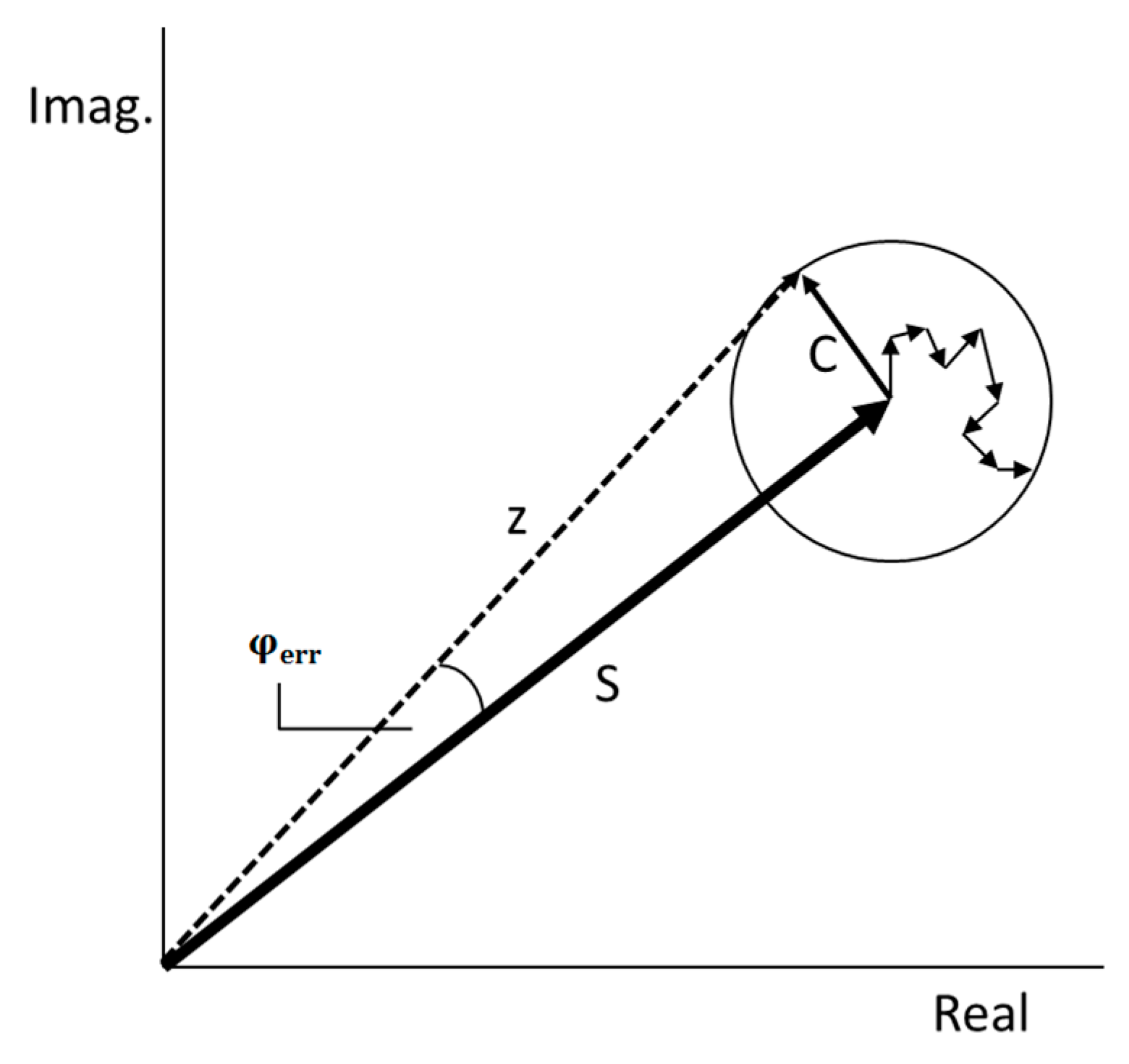
The complex radar observation at each pixel is the coherent sum of the response from many distributed scatterers located within that pixel. Deformation studies using differential InSAR techniques exploit the phase component of the complex radar signal. The phase for pixels containing distributed scatterers (i.e., those that are un-correlated and where no single scatterer dominates) is unlikely to remain correlated for long periods of time. The PSInSAR technique only exploits those pixels within which there is a dominant scatterer, the so called “PS”, exhibiting long-term stable phase characteristics. The phase component from the PS depends on the range (distance) from the target to the SAR sensor whereas the phase due to the other distributed scatterers within the pixel is essentially random (Figure 1).
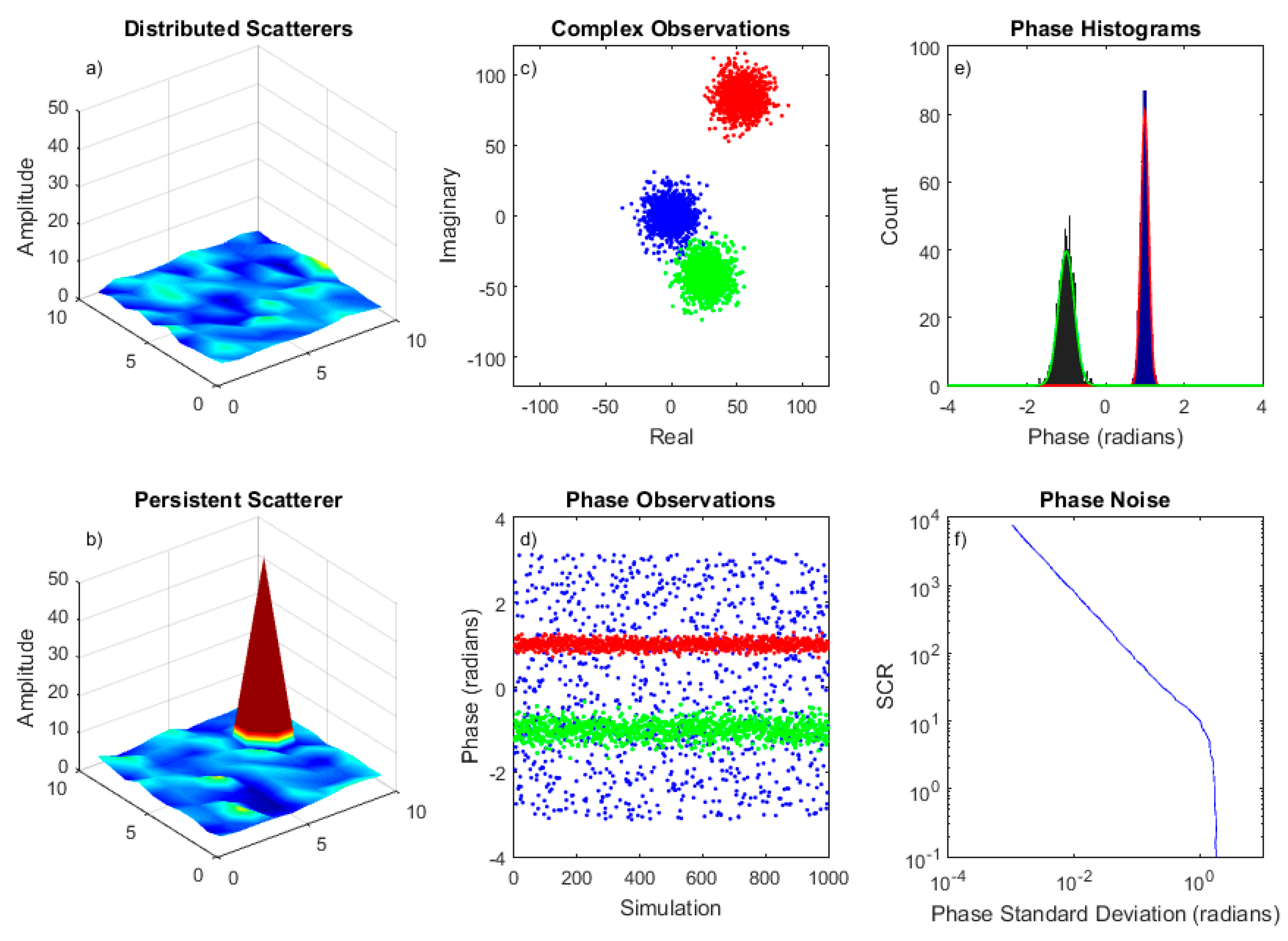
A simulation of the phase response for a single SAR image pixel comprising many uncorrelated distributed scatterers under the assumption of a complex circular Gaussian statistical model is presented in Figure 2. Under these conditions the amplitude and phase probabilities are approximated by Rayleigh and uniform distributions, respectively [6]. The simulation is repeated twice with the presence of a single PS replacing a distributed scatterer within the pixel. The PS has an amplitude response of about four and eight times the background amplitude in the two further simulations (i.e., an SCR of about 16 and 64, respectively) and a defined phase. What can be seen is that with no PS the phase is uniformly distributed between ±π. The effect of adding the PS is to reduce the level of phase variability in proportion with the amplitude of the PS. As can be seen in Figure 2e, the normal distribution is only a crude approximation to the phase statistics. An important observation is that the phase standard deviation (derived from the best-fitting normal distribution to the phase observations) decreases as the SCR increases (Figure 2f). Below an SCR of about 10 (i.e., ~10 dB), the phase can no longer be adequately approximated by a normal distribution [23]. This is demonstrated in Figure 2f, where below an SCR of 10 the phase standard deviation stagnates, indicating that a uniform distribution of phase values prevails.
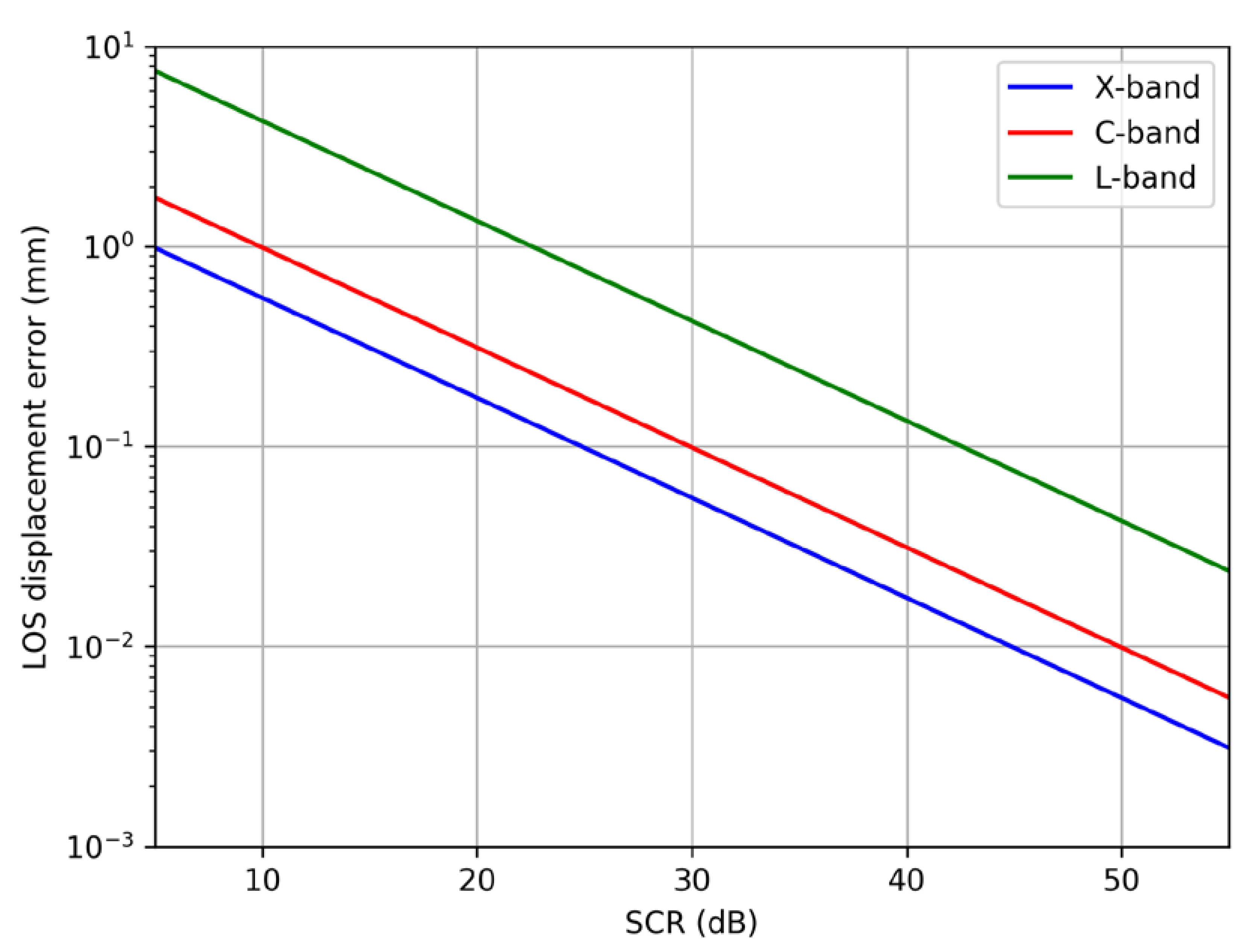
Using this simple analytical expression, the estimated phase error can be directly derived from the measured point target SCR in any single SAR image. Furthermore, the SCR and phase error is dependent only on the image resolution and the radar frequency. It is therefore useful as an a priori metric during network design when a large number of SAR images may not yet be available for a particular area of interest and therefore direct interferometric measurements are not feasible. The estimated phase error can be converted to a displacement error in the line of sight (LOS) using the radar wavelength :
The relationship between the SCR and LOS displacement error is plotted in Figure 3 for the radar bands generally used on current SAR missions.
2.3. Target RCS Requirements
By considering the expected background pixel RCS for the SAR imaging mode to be used, an RCS requirement for deployed targets can be derived based on an acceptable level of displacement error (due to random phase error alone). The RCS of a pixel is equal to the product of the illuminated ground range resolution area and the clutter intensity. The required RCS for the target is then found by multiplying the derived pixel RCS with the SCR (in the linear domain; cf. Equation (3)). As an example, I derive approximate values for the RCS of artificial targets that would achieve a nominal LOS displacement error not greater than a tenth of a millimetre in different imaging modes of the currently orbiting SAR sensors (Table 1). A 0.1 mm magnitude of error would require an SCR exceeding 25 dB, 30 dB and 43 dB at X, C, and L-bands, respectively (Figure 3).
For the purpose of classification in this paper, “high-resolution” image modes are those with a ground range resolution area less than 5 m2, “medium-resolution” are those between 5 m2 and 100 m2, and “low-resolution” are those above 100 m2. Based on the pixel RCS values calculated in Table 1 and the identified SCR requirements, the artificial target must have an RCS up to 31 dBm2 for medium-resolution X-band SAR imagery, 37 dBm2 for medium-resolution C-band SAR imagery, 41 dBm2 for low-resolution C-band SAR imagery (excluding Sentinel-1’s Extra Wide Swath mode), and 47 dBm2 for medium-resolution L-band SAR imagery.
2.4. Target Design
A radar reflector is a passive device that reflects incoming electromagnetic energy directly back to the source of that energy. There are many different types of reflectors, including: spheres, cylinders, dihedrals, trihedrals, flat plates, top hats and bruderhedrals. A trihedral radar reflector (often known as a “corner reflector”) facilitates a triple-bounce of the incident radar energy from three mutually orthogonal plates [25]. The RCS pattern of a trihedral has a 3 dB beam-width of approximately 40° [20,26]. This means that a trihedral design is much more forgiving of field alignment errors when compared to other reflector designs. Consequently, trihedral corner reflectors have been used for many years as targets suitable for calibration of SAR images (e.g., [19,27,28,29]) and they are also the most common target type being deployed for use in PSInSAR analysis of ground deformation.
The shape of the reflecting plates impacts on the RCS magnitude of a trihedral corner reflector. The most commonly used plate shape is the triangle, but square and quarter-circle shaped plates have also been used [10,30]. Of these shapes, the triangle has the lowest RCS for a given size, but has the advantage of being structurally rigid and easy to manufacture. Sarabandi and Tsen-Chieh [31] described ‘optimum’ corner reflectors with pentagonal-shaped plates, created by trimming the ineffective part of a triangular plate that does not contribute to the RCS pattern. However, this trimming complicates the manufacture process and reduces the overall rigidity of the corner reflector. For these reasons, the focus of this paper is on the triangular trihedral corner reflector, hereafter abbreviated TCR. The theoretical peak RCS value () of a TCR (expressed in m2) is given by [32]:
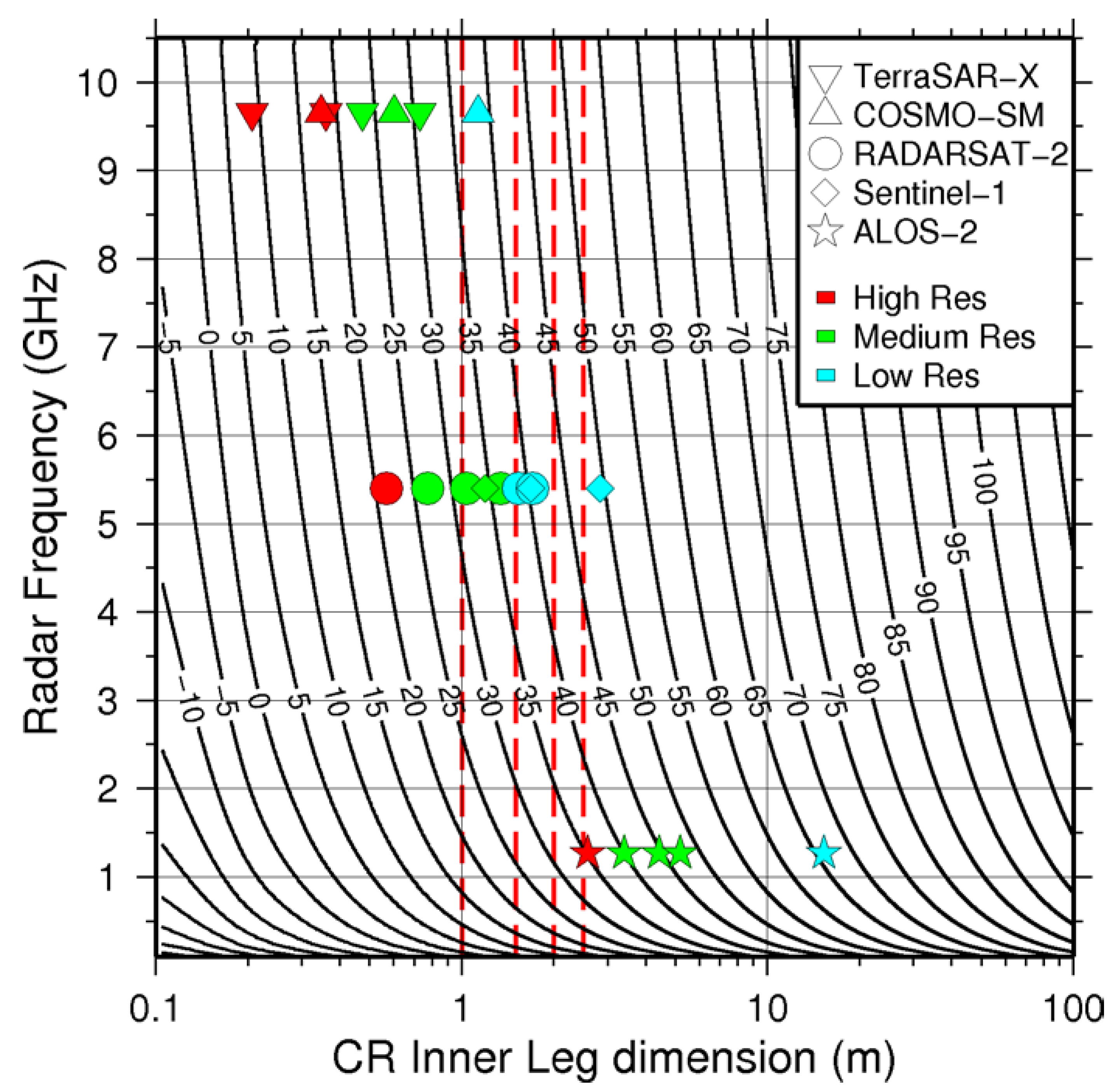
where is the radar wavelength and is the length of the non-hypotenuse sides of the right-angled isosceles triangular plate (the inner-leg dimension). Using this relation, the equivalent size of TCR required to meet the RCS requirement of the design tolerance (0.1 mm LOS displacement error) is given in Table 1. Due to the frequency dependence of the RCS response, the design requirement results in non-overlapping size specifications for TCR (Figure 4). At X-band, TCR with an inner-leg dimension of 0.7 m should theoretically be able to achieve the displacement error tolerance for all medium-resolution image modes. At C-band, medium and low-resolution modes require a TCR dimension of between 0.8 m and 1.7 m. At L-band medium-resolution modes require a dimension of 5 m or greater.
It is therefore necessary to make a compromise if more than one SAR frequency is to be exploited using the same target. The compromise should be made at the higher frequency, since it is better for a target to be too bright but still visible rather than too dark and not visible. Due care and consideration should be taken to ensure that the target design will not saturate the signal, particularly at higher frequencies. As an indication of ‘safe’ target sizes, the German Aerospace Center (DLR) report usage of 3.0 m TCR for calibrating the TerraSAR-X sensor without saturation [28]. Furthermore, DLR have designed a C-band transponder with an RCS of 60.8 dBm2 for calibration of Sentinel-1 and tested using RADARSAT-2 [33]. This is equivalent to a TCR with an inner-leg dimension of approximately 5.5 m. If a 5.5 m TCR were used at L-band (for example, with ALOS-2 Stripmap Fine data) a 0.1 mm LOS displacement error could be achieved. It is therefore possible to obtain a sub-millimetre LOS displacement error at L-band without saturating the signal at X- or C-band. However, the large size of TCR required to achieve sub-millimetre LOS displacement error at L-band could be impractical for widespread use in geodetic networks.
3. Manufacturing and Design Considerations
3.1. Losses Due to Manufacturing
There are several factors that can introduce a loss of RCS for a TCR compared to the theoretical values given by Equation (6), including inter-plate orthogonality, plate curvature and surface irregularities. To achieve an RCS accuracy of better than 1 dB with respect to theoretical values, DLR specify the following tolerances on their TCR manufacture process: Inter-plate orthogonality ≤ 0.2°; Plate curvature ≤ 0.75 mm; Surface irregularities ≤ 0.5 mm [28]. These tolerances apply to X-band, with less stringent tolerances applying to lower frequencies.
The inter-plate orthogonality is the extent to which the three plates form 90° angles at their intersections. Robertson [34] conducted a series of physical experiments to measure the RCS profile of trihedral reflectors when the inter-plate angles are varied from 90°. When only the angle between the two vertical plates is varied, the azimuth profile flattens. Furthermore, the peak RCS is less, with the loss being more severe when the inter-plate angle is less than 90°. Robertson [34] also found that the RCS loss effect of inter-plate angle variation is more severe as the size of corner reflector increases (cf.) [35] and the radar wavelength decreases. Sarabandi and Tsen-Chieh [31] found that for distorted triangular, square and pentagonal plated corner reflectors the relative loss of RCS is between 0.2 dB and 1 dB for an angular deviation of ±1° and between 1.3 dB and 2.8 dB for ±2°. Again, the losses are more severe when the inter-plate angle is acute rather than obtuse. These results indicate the importance of ensuring 90° angular relations between the intersecting plates of a corner reflector during manufacture but also through transportation and installation.
Plate curvature is the deformation of the plate from a perfectly flat plane along its entire length, such as a gradual warp across the plate. In general, RCS loss due to plate curvature is inversely proportional to the radar wavelength and the target size. An RCS loss exceeding 10 dB can result from a 5 mm plate curvature in a 1.0 m trihedral corner reflector at X-band [35].
Plate surface irregularities are the presence of any small-scale feature that causes a deviation from perfect flatness at any given location across the plate. Usage of fasteners such as pop rivets or retaining bolts on any of the plates reflecting surfaces could affect the RCS performance of the target. The RCS loss is proportional to the surface deviation across the plate and inversely proportional to the radar wavelength. A surface feature of only 1 mm deviation could introduce a 1 dB loss at the X-band [35].
3.2. Other Design Features
The material and finish to be used to manufacture the corner reflector plates also needs consideration. Aluminium is commonly used for the construction of plates. Aluminium is generally more costly than steel, but it does not suffer as badly from corrosion and is relatively lightweight. A plain metallic finish should achieve the best radar reflection properties. A thin thermoplastic powder-coat layer may assist in ensuring the longevity of the corner reflector when deployed by resisting oxidation and degradation of the metal but it will introduce RCS losses. Another design feature worth considering is whether to use pre-fabricated mesh sheeting or adding perforations to solid metal sheet. Introducing a large number of holes in the plates has the benefit of allowing quick drainage during heavy rainfall, relieving some of the force applied to the structure by wind, reducing overall weight and promoting self-cleaning of dust and other wind-blown deposits. The addition of holes to the plates will reduce the RCS, with the hole size and spacing both having an impact. To keep RCS losses below 1 dB, the hole diameter must be less than about one-sixth of the radar wavelength (Cheng Anderson, Defence Science and Technology Organisation (DSTO), Pers. Comm. 2012). For utility at X-band, the maximum size of perforation should therefore not exceed 5 mm. Measurements made by DSTO indicate an RCS loss of 0.2 dB and 1.2 dB for mesh samples with 5 mm diameter holes and a ~20% open (non-metallic) area for C and X-band, respectively [36]. Note that using a physical punch to add holes to sheet metal could affect the plate curvature and/or introduce surface irregularities.
Even if mesh or perforations will not be used, it is recommended that several holes are introduced close to the trihedral apex to allow precipitation to drain. Flooding of the corner reflector will introduce an RCS loss at least an order of magnitude greater than that caused by the presence of holes in the plate due to the breakdown of the triple bounce reflection mechanism within the TCR aperture. For example, during the field experiment described in this paper a build-up of dirt blocked the single drainage hole in one TCR prototype, which subsequently caused that TCR to fill with water following a heavy rainfall event. The resulting drop in RCS measured in two X-band COSMO-SkyMed images spanning the rainfall event was 13.2 dBm2 (±0.69 2-sigma).
3.3. Target Characterisation
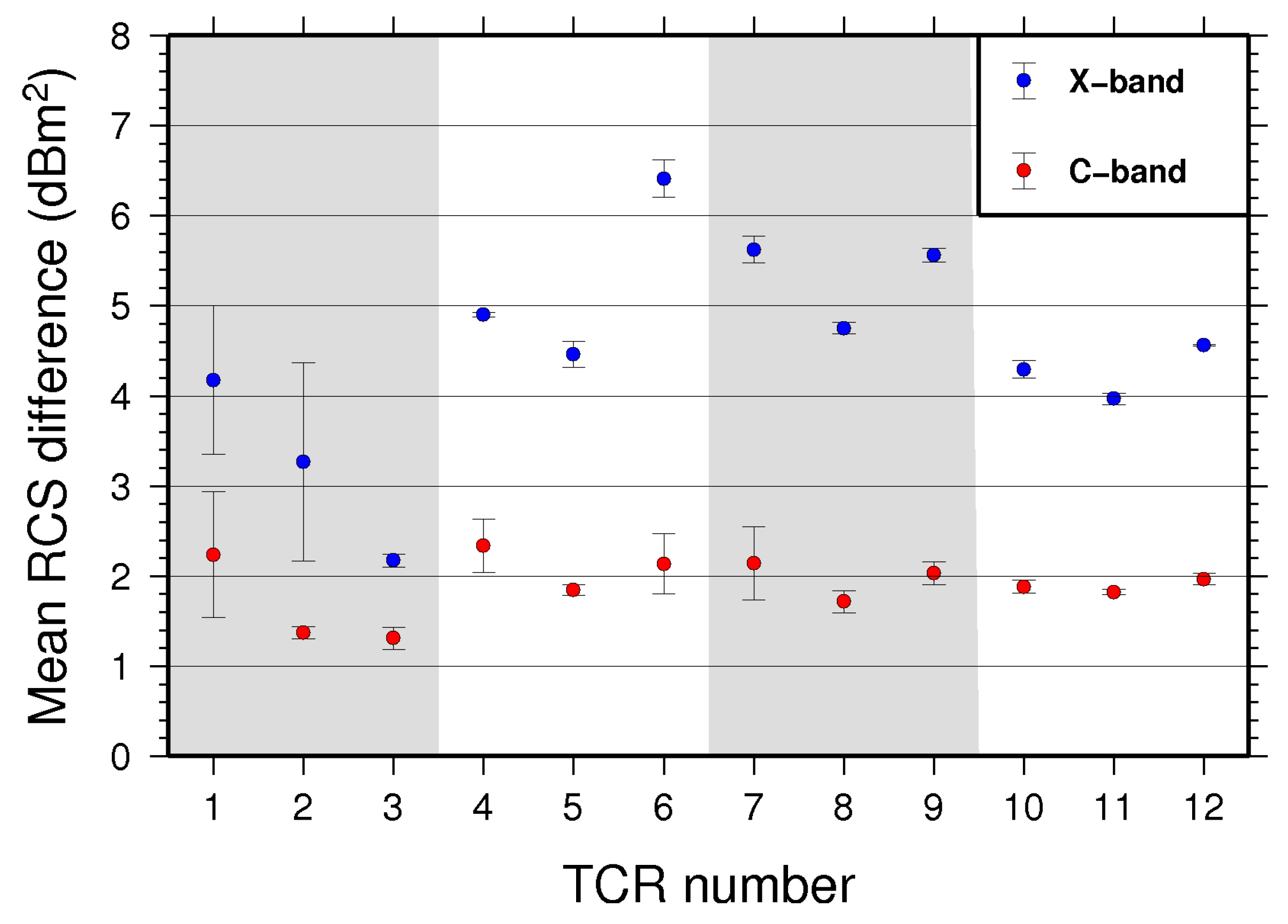
As a prelude to the experiments reported here, Geoscience Australia [36] described X and C-band RCS characterisation measurements made at a ground radar reflection range on 12 TCR prototypes of four different designs: 1.0 m solid metal sheet; 1.5 m solid metal sheet, 1.5 m powder-coated solid sheet; 1.5 m with perforated plates (15.7% open area and 5 mm diameter holes). The same twelve TCR prototypes were used in the field experiments reported in this paper, and the different designs correspond to the “type groups” A, B, C and D reported in Table 2. Three of each design were manufactured and characterised to test the consistency of the manufacturing process. The results of these measurements (Figure 5) show that there is good consistency between individual TCR regardless of plate finish, particularly at C-band where 1.5 m TCR have an RCS of 2.0 ± 0.3 dBm2 less than theory and 1.0 m TCR are around 1.6 +0.6/−0.3 dBm2 less than theory. At the X-band the RCS of individual TCR is more variable, ranging between 5.0 +1.5/−1.0 dBm2 less than theory for 1.5 m TCR and 3.2 ± 1.0 dBm2 less than theory for 1.0 m TCR. Since several distortions of the tested TCR have been documented [36], these results confirm that departures of the TCR from perfect inter-plate orthogonality and plate flatness are less tolerated at shorter radar wavelengths and, in the case of plate curvature, is more severe for smaller targets.
4. Field Experiments
In this section I describe field experiments that were conducted using prototype TCR with inner-leg dimensions of 1.0, 1.5, 2.0, and 2.5 m to test whether the theoretically-derived performance (defined by RCS, SCR and LOS displacement error) is achievable in a typical deployment environment in Australia. As indicated in Figure 4, the range of TCR sizes manufactured for this experiment spans the requirements of medium- and low-resolution X- and C-band SAR imaging modes. At the time of this experiment L-band SAR data was not readily available from any sensor (the Japanese ALOS-2 satellite was launched after the conclusion of the field experiment). Correspondingly, L-band is not discussed any further in this paper.
4.1. Test Site
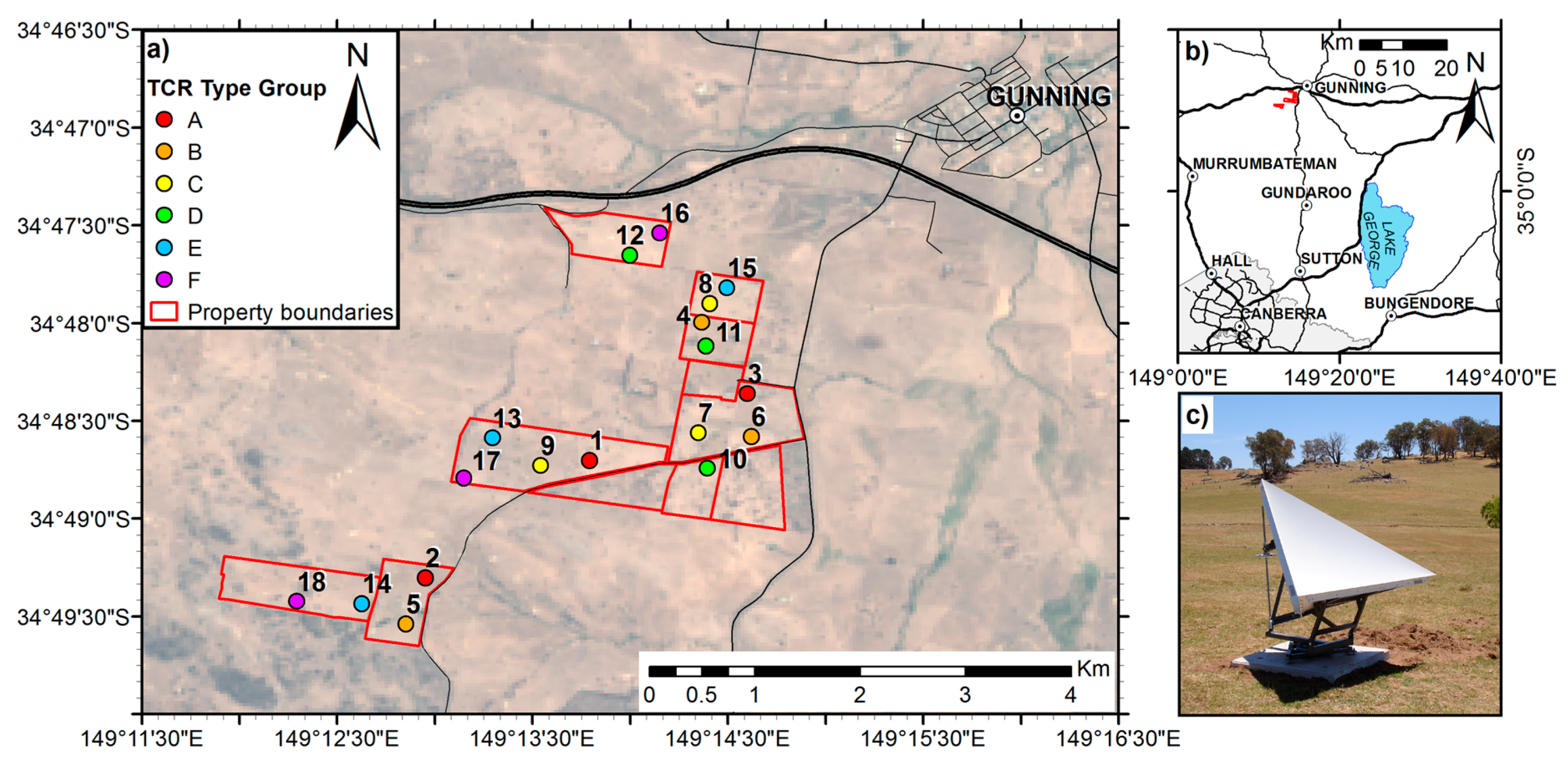
Eighteen TCR prototypes (including the twelve TCR tested at the ground radar reflection range, see Figure 5) were deployed in a temporary array on a grazing property near Gunning, New South Wales, for a period of five months between December 2013 and May 2014 (Figure 6; Table 2). Several factors were considered when choosing installation sites for each TCR, including the flatness of the site and immediate surrounds, the perceived sources of clutter near to the site and the distance from metallic boundary fences. The TCR were also carefully positioned in such a way that the impulse response in the SAR imagery would not overlap with or intersect the response from adjacent TCR sites. The baselines between all TCR deployment sites were 186 m or greater.
4.2. Target Alignment
The TCR boresight is the vector of the maximum RCS response emanating from the internal intersection of the reflector plates (the apex). From physical optics, the boresight vector for any trihedral target is oriented 45° from the two vertical plates, and elevated 35.26° from the baseplate [26]. Misalignment of the TCR boresight with respect to the SAR sensor boresight will incur a loss of RCS. In the field, the TCR must be aligned in azimuth and elevation so that the boresight vector is oriented toward the LOS of the orbiting SAR platform of interest, including consideration of any squint angle of the SAR sensor. The required orientations can be calculated using published orbital information for the SAR platforms of interest, and the deployment position of the target [36]. For a particular orbital pass direction (ascending or descending), the azimuth alignments for the SAR sensors in Table 1 only vary by ~1°, whereas the elevation may vary by much more depending on the incidence angle of the swath and image mode chosen. Typically, the imaging modes have incidence angle ranges of at least 25°. An incidence angle range of 20–45° results in a pixel RCS variation of 3.2 dBm2 across this range, independent of imaging resolution. Therefore, if the choice of imaging sub-swaths to be used is carefully considered, one target alignment can be used for multiple SAR sensors with only marginal difference in RCS between sensors because of imaging geometry.
Alignments were calculated for the viewing geometry of each SAR sensor, and an average of these three geometries. The boresight of each TCR was re-oriented to these alignments prior to each satellite overpass according to the notes in Table 3.
4.3. SAR Imagery
Twenty-two SAR image acquisitions at X and C-bands were made using the TerraSAR-X (TSX), COSMO-SkyMed (CSK) and RADARSAT-2 (RSAT-2) SAR systems (Table 3). All SAR images used in the analysis are HH polarised and were acquired on descending passes. In total, nine TSX Stripmap mode “SSC” images, nine CSK HIMAGE mode “SCS_B” images and four RSAT-2 Fine mode “SLC” images were acquired for the field experiment (Table 3). The beam modes used (9, 5 and 21, respectively) resulted in average local incidence angles at the TCR deployment sites of 35.22°, 33.31° and 34.90° for TSX, CSK and RSAT-2, respectively. TSX products were ordered with a −10 dB gain attenuation and RSAT-2 products were ordered with the Calibration-2 look-up table to ensure the dynamic range of the SAR data could accommodate the impulse response of even the largest 2.5 m TCR present in the imaged area. An example of the impulse response from each size of TCR in a TSX image is shown in Figure 7.
4.4. Image Processing Methodology
I used the GAMMA software [37] to process the received Single Look Complex (SLC) imagery for each SAR sensor before applying the integral method [38] to compute the RCS of each TCR in each image. The integral method is commonly used to determine the absolute calibration factor for SAR imagery by measuring the radar response of targets of known RCS. Since the received SAR imagery is already externally calibrated, the procedure is simply reversed in order to determine the RCS of the TCR. The procedure used is as follows:
- Read the SLC imagery and convert to Sigma Nought. For TSX and CSK this involves applying the annotated product calibration factor and then scaling the image by to get Sigma Nought. For RSAT-2 this involves applying the provided Sigma Nought look-up table.
- For each SAR sensor, coregister all SLC images to a single master image (chosen to be the earliest acquisition). Verify the co-registration of each image and determine the range (column) and azimuth (row) coordinates of each TCR in the co-registered images.
- Define a ‘target window’ that encompasses the impulse response of the target and four ‘clutter regions’ in the quadrants surrounding the side lobe response of the target (Figure 7b).
- Determine the mean signal clutter in the four ‘clutter regions’. By computing the clutter level as the mean of all pixel values falling within standard-sized windows, a representative view of the actual reflector RCS and SCR is obtained that removes any bias associated with the common practice of manually choosing the location of windows to sample only the lowest clutter in the general surrounds of the target.
- Calculate the integrated point target energy:where is the integrated (summed) energy in the ‘target window’, is the total integrated energy in the four ‘clutter regions’, is the number of samples contained within the four ‘clutter regions’ and is the number of samples in the ‘target window’.
- Compute the RCS of the point target by multiplying the integrated point target energy by the area of the ground range resolution cell:
- Compute the SCR; the ratio between the point target energy corrected for clutter and the average clutter level per pixel:
- Compute the phase error (Equation (4)) and convert to LOS displacement error (Equation (5)).
5. Results
In this section I will describe the results of the TCR field experiments in terms of the radar clutter, RCS, SCR and derived LOS displacement errors detected at the deployment sites.
5.1. Clutter Intensity
In general, the average clutter levels at Gunning were between −11 dB and −16 dB for both X- and C-band (Figure 8). The clutter level is roughly the same for both X- and C-bands, consistent with the expectations discussed previously. There is a larger variation in clutter values between TCR sites in the RSAT-2 imagery, which may be because of the coarser pixel resolution resulting in greater speckle variation compared with the higher resolution X-band imagery.
There is a strong correlation between rainfall and trends in clutter intensity for all SAR sensors (Figure 8). Significant rainfall occurred in early November 2013, prior to the installation of TCRs at Gunning. Following this time, a period of mainly dry conditions ensued until February 2014, interspersed by sporadic rainfall events of 1 day duration and around 10 mm or less. During this time, ground conditions at the Gunning test site were observed to become drier, whilst vegetation dried out and the overall volume of biomass reduced. Between 14 to 17 February 2014, ~60 mm of rain fell during a four-day period. Corresponding increases in soil moisture resulted in an increased clutter intensity in imagery from all three SAR sensors. The total increase in clutter following the February rainfall event was about 2–3 dB for TSX with a similar increase inferred for CSK and RSAT-2.
Prior to March 2014, all CSK acquisitions were made using satellite #1 of the constellation. In March and April 2014, four further CSK acquisitions were made using a combination of satellites #1, #2 and #4. Average clutter intensity had a range of ~1.5 dB between these four acquisitions. It is difficult to draw objective conclusions about an inter-constellation comparison from this observation due to the significant amounts of rainfall that fell between adjacent acquisitions that could majorly impact the backscattered signal.
5.2. Radar Cross Section
Figure 9 shows the RCS measured in SAR images for each deployed TCR and a comparison with theoretical RCS values for each size of target. Between mid-December 2013 and mid-February 2014, the background clutter at X and C-bands is consistently low (−16 to −14 dB; Figure 8). Therefore, only images acquired within this time period with relatively stable background clutter were used to calculate a mean RCS (and measurement standard error) for each TCR (see Table 3). The estimated RCS values for many TCR in RSAT-2 images turn out to be greater than theory. This situation is not a possibility, and it highlights that the calibration of RSAT-2, and indeed any SAR system, is performed using different methods and software. It is therefore not likely that equivalency is being compared between the signals from RSAT-2, CSK and TSX. When considering the measured RCS values of these three systems, it appears that CSK is performing the worst because it is the most different to the theoretical RCS values. The relative differences between the three SAR systems are consistent across all TCRs. There is a mean difference of 1.32 dBm2 (±0.08 2-sigma) between TSX and CSK.
There are no consistent differences in RCS that can be attributed to the differences in plate finish of the 1.5 m TCRs. Since variations in RCS within each TCR type-group is correlated across different SAR sensors (particularly TSX and CSK) it appears that site-specific conditions are having a larger impact on measured RCS. Variability of RCS within type-groups is again more pronounced at X-band as was the case in the ground radar reflection range measurements (Figure 5).
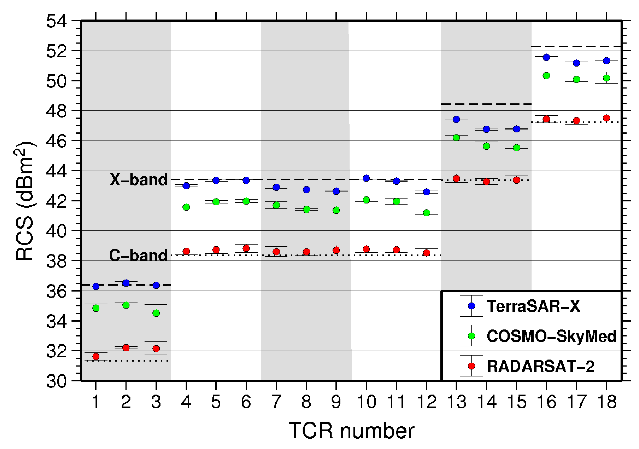
Generally, the RCS difference between observations and theory reduces in proportion with the TCR size. This is more apparent at X-band; for TSX the difference between smaller and large TCR is on the order of 1.0 to 1.5 dBm2 and for CSK is on the order of 0.6 to 1.1 dBm2. The trend is not as obvious in C-band (RSAT-2) RCS estimates. This could be reflective of the fact that departures from inter-plate orthogonality and plate flatness are tolerated less at shorter radar wavelengths. It could also be indicative that for the larger TCR, the ‘target window’ used to sample the impulse response is not fully capturing the full extent of side lobes, which are much broader for the 2.0 m and 2.5 m TCR (e.g., Figure 7). Consequently, the RCS measurements for the larger TCR could be adversely biased to be less than the true RCS because of the sampling choice.
5.3. Impact of Misalignment
In a secondary experiment, certain TCR were purposefully misaligned from the optimum calculated boresight for at least one acquisition of each sensor (see Table 2) to measure the RCS loss as a result of these misalignments in consecutive images from each SAR sensor (Figure 10). To ensure consistent inter-constellation signal level, images from the CSK-1 satellite were used. Four TCR, one of each size, were used as ‘control’ and were not misaligned and so theoretically should exhibit a zero RCS loss. In practice, the difference is not zero due to temporal clutter changes occurring between the two acquisitions. To partially account for this, the standard error of the difference in RCS measurements for these four control TCRs (numbers 3, 5, 13 and 16) were used to derive error bars for the other RCS loss measurements.
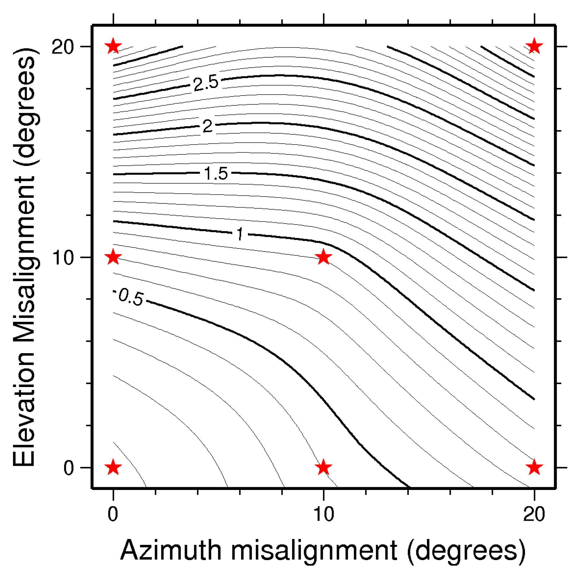
It is clear from these results that RCS loss is mainly dependent on alignment error rather than TCR size. For instance, all the TCR with an elevation misalignment of 20° (TCR numbers 2, 4, 6, 9, 14 and 18) suffer an RCS loss of 3–4 dBm2 regardless of size. The level of RCS loss is comparable (within measurement error) in TSX, CSK and RSAT-2 images for all TCR sites, and therefore is not dependent on radar frequency. The other notable observation is that RCS loss is more severe for elevation misalignments than equivalent azimuth misalignments. Furthermore, the greatest RCS loss is seen for TCR 9 which has the worst misalignment (20° in both elevation and azimuth). Figure 11 summarises the impact of these azimuth and elevation misalignments from the optimum boresight direction. In general, the observations at X- and C-band imply that if azimuth and elevation alignment accuracies of 10° are adhered to, the resulting RCS will be within 1 dB of the peak value. Furthermore, a realistic alignment accuracy of a few degrees [36] would result in an RCS loss of less than about 0.2 dB.
5.4. Displacement Error
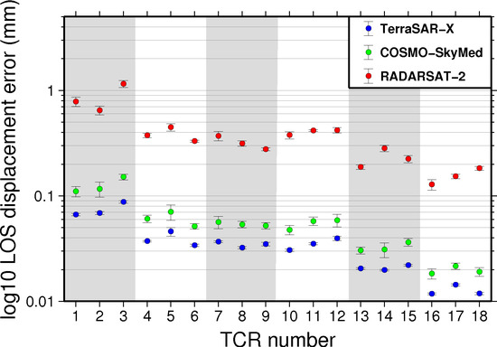
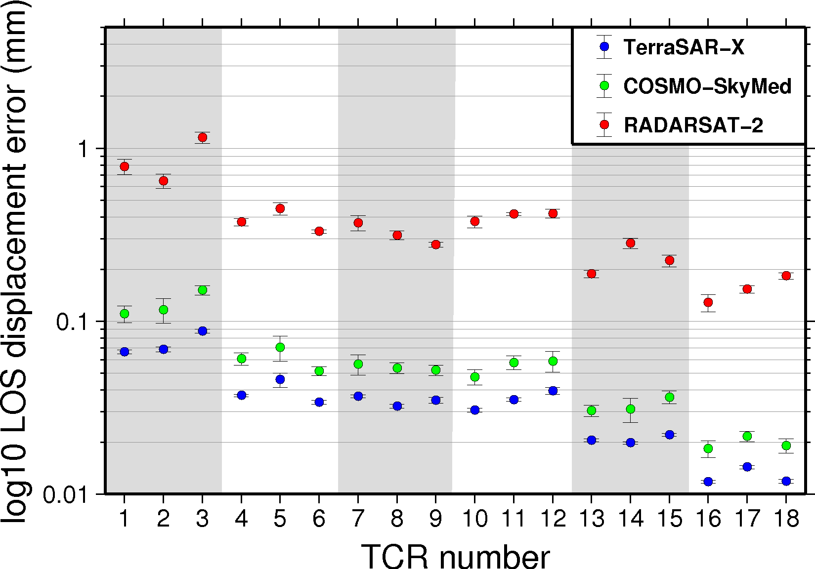
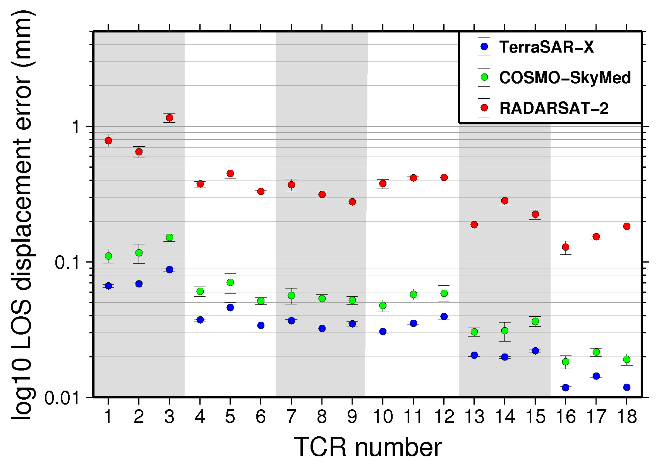
Figure 12 shows the LOS displacement errors derived directly from measurements of the SCR from SAR imagery at Gunning. As for RCS measurements, only images acquired within the time period with relatively stable background clutter were used to calculate a mean LOS displacement error (and measurement standard error) for each TCR (see Table 3). Generally, we see that the LOS displacement error decreases with TCR size as expected since SCR is proportional to TCR size for a fixed clutter magnitude. The LOS displacement error is also frequency dependent, with C-band having greater displacement errors than X-band for the same TCR. At X-band, all TCR larger than 1.0 m meet the nominal design LOS displacement error criteria of 0.1 mm. The 1.0 m TCRs also meet this criterion in TSX imagery, but not in CSK. In fact, all TCRs have an SCR consistently about 4 dB less in CSK imagery than in TSX imagery. At C-band only the 2.5 m TCRs come close to the design criteria of 0.1 mm, although all TCR larger than 1.0 m have a LOS displacement error less than 0.5 mm. According to the theoretical calculations in Table 1, the 2.5 m TCR should exceed the 0.1 mm LOS displacement error. The fact that it does not highlights that in general the TCR prototypes are not performing as well in real data as in our expectations.
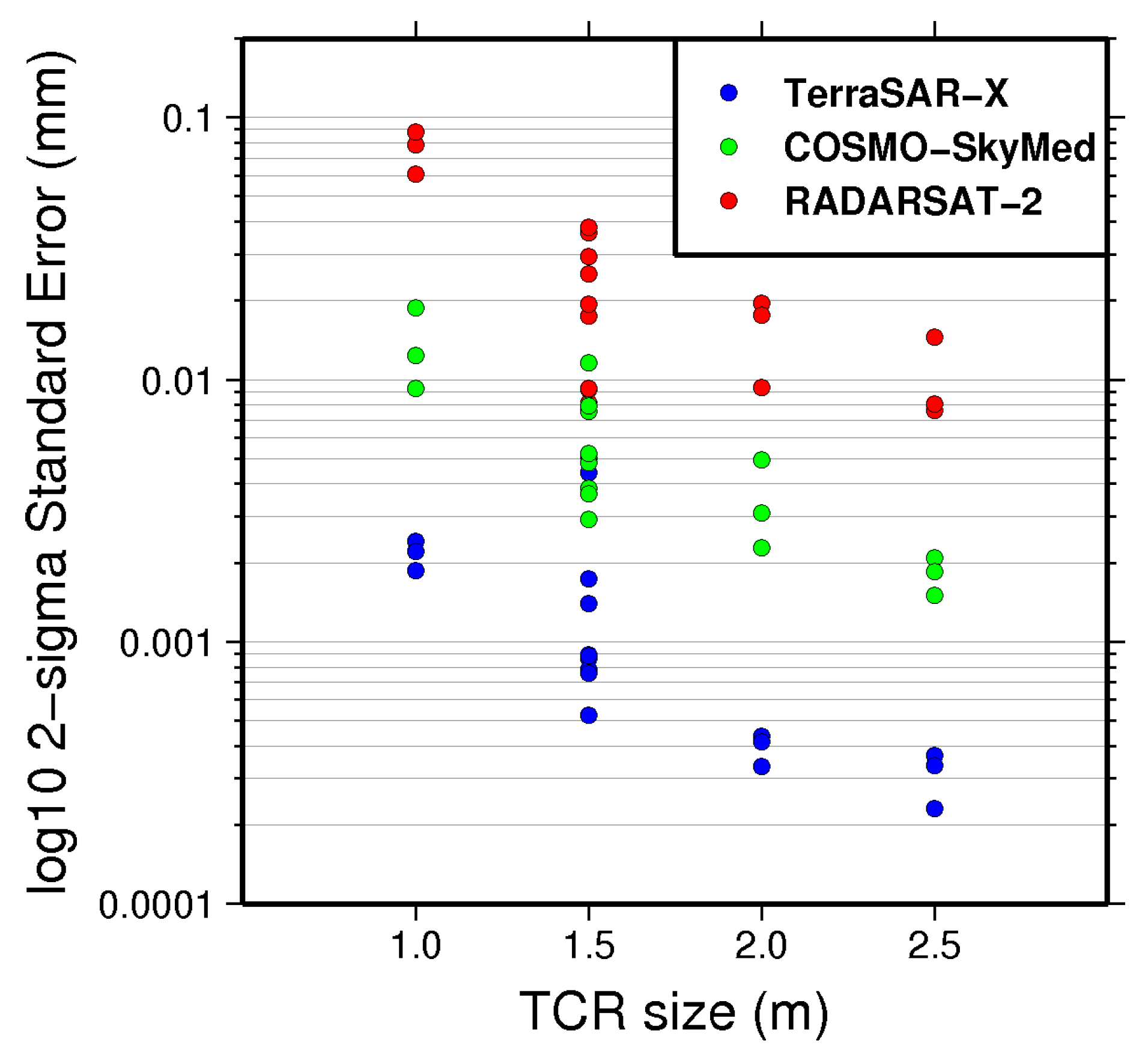
The magnitude of the 2-sigma standard errors on the LOS displacement error estimates are plotted against TCR size in Figure 13. There is a clear relationship between TCR size and variability of displacement error (and implicitly SCR) with a consistent exponential trend between sensors. This confirms the theoretical phase noise behaviour demonstrated previously in the PS phase simulation (Figure 2) whereby the phase noise becomes less variable as the SCR increases in concert with an increase in target size.
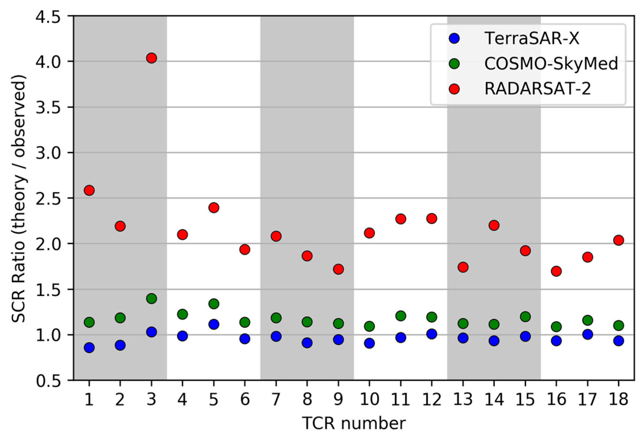
Figure 14 shows the ratio of the theoretical SCR against observed SCR values derived using Equation (9) for the TCR deployed at Gunning. Theoretical SCR is calculated using the average observed clutter at each TCR in those images highlighted in Figure 8 and Table 3 (corresponding to relatively stable clutter characteristics) and the ground range resolution area derived from the pixel resolution. With an average ratio close to 1, the TCRs are performing close to expectations in TSX images. In CSK this ratio is marginally worse at ~1.2. In RSAT-2 the ratio is much worse at ~2.2. Interestingly the ratio between SCR observations and theory is consistent across all TCRs for TSX and CSK, though in RSAT-2 the ratio is variable, with larger TCR performing better. This indicates that TCR between 1 m and 2.5 m size are adequate for use with TSX Stripmap and CSK HIMAGE imagery if the goal is to achieve a phase noise error equivalent to a tenth of a millimetre displacement in the line of sight. Only the larger TCR are close to achieving that criterion in RSAT-2 Fine imagery.
6. Discussion
TCR performance is clearly limited by the choice of deployment site. For instance, TCR number 3, a 1.0 m target, was situated in a position relatively close to distributed metallic debris and farm buildings. The impact of this background clutter at the deployment site on SCR performance is self-evident in Figure 12 and Figure 14. Furthermore, the effect of the increased background clutter was compounded in this case by the relatively small size of the target deployed at this site. This highlights the importance of choosing clutter-free sites for deployment of targets to be used as geodetic targets whenever feasibly possible.
The results presented here show that there are differences between the backscattered signal measured by CSK and TSX. The fact that TSX has higher RCS than CSK is consistent with previous work where a mean backscattering difference of 3.15 dB between TSX Stripmap and CSK HIMAGE images was identified [39]. While these inconsistencies may be attributed to the absolute radiometric calibration of the two systems, there are other reasons for at least some component of the observed differences. As reported previously, the average local incidence angle across all the TCRs in all the images is 35.22° in TSX and 33.31° in CSK. This 2.1° difference in incidence angle results in a backscatter difference of 0.2 dB purely due to differences in the viewing geometry, though taking into consideration the difference in spatial resolution of TSX Stripmap and CSK HIMAGE images the deviation could be as much as 1.7 dB. The standard deviation of the local incidence angles infers that the satellite orbital path varies more for CSK (or RSAT-2) in comparison to TSX. The standard deviations across all images used in this experiment are 0.051° for CSK, 0.008° for TSX and 0.044° for RSAT-2.
Another possible explanation for observed discrepancies between SAR sensors is the different processing applied to the raw SAR data during SLC production by the data providers. Interestingly, the extent of side-lobe ringing from TCRs deployed at Gunning is visually more pervasive in CSK images when compared to TSX images. For the purpose of a ‘fair test’, a fixed ‘target window’ size was used to determine the RCS of TCRs across all sensors. As a consequence, it is certainly possible that not all the reflected energy pertaining to the TCR is sampled. This would give rise to a bias in the measured signal, which in the case of CSK data (with the larger side lobes), could manifest as a reduced RCS and SCR measurement.
The ground radar reflection range measurements of twelve of the TCR prototypes deployed at Gunning indicate RCS performance in the −2 to −5 dBm2 with respect to theoretical values (see Figure 5). It is interesting that the measured performance in the satellite SAR data is better (Figure 9). Several compromises that were made during the ground measurement procedure (documented in [36]) are the likely reason for these discrepancies.
Using the SCR as an a priori proxy for phase error, and therefore LOS displacement error, should be treated with some caution. Ketelaar et al. [23] conducted a validation experiment with five corner reflectors, comparing heights derived from ERS and ENVISAT InSAR analyses with repeated levelling surveys. From this experiment, they found that the SCR-derived phase error is under-estimated by up to four times compared to the levelling measurements. An alternative method for estimating the phase error, commonly used during candidate PS selection in the PSInSAR workflow, is the amplitude dispersion method [1]. Through a simulation exercise, [24] find that the SCR is a more effective estimator of phase error than the amplitude dispersion when the SCR is greater than 9 dB. Below this threshold, both methods are optimistically biased, with the amplitude dispersion being more so. When using the amplitude dispersion method to select candidate PS pixels during PSInSAR analysis, generally at least 20 SAR images are required to achieve an unbiased estimate of the phase error [24]. Therefore, the small number of SAR images acquired with each sensor during the Gunning field experiment precludes conducting a robust interferometric analysis using this data. However, I consider the estimated LOS displacement error as a suitable quantity with which to relatively assess different TCR designs.
Compact, active transponders (as described by [13]) are an alternative type of artificial target to corner reflectors that can be deployed readily in geodetic networks and utilised with C-band sensors such as Sentinel-1 and RSAT-2. The clear advantage of these transponders over passive corner reflectors is that they are consistently compact and therefore less obtrusive in the environment and more easily coupled (due to their small size) to other geodetic monumentation for cross-validation of signals. The RCS of these transponders is restricted to a narrow band of a few hundred MHz since they are designed to target specific SAR sensors. Therefore, the existing transponder designs cannot be used as a single point of reference across multiple frequency bands in the same way as a corner reflector. One other consideration is that transponders are active transmitting devices and therefore require a power supply for long term deployment and an appropriate radio transmission licence to be operated. These may be difficult and expensive to obtain in some jurisdictions.
The Sentinel-1 SAR constellation mission [40] has brought about a new era for SAR remote sensing in which open access to data acquired with blanket global coverage at frequent and regular revisits is becoming a reality. To some extent SAR missions like Sentinel-1 removes the need for radar targets to perform adequately at multiple frequencies, and in this situation it is much easier to design a target towards a specific level of displacement error without the need to make compromises for different SAR frequencies. Generally, this will enable the designed target to be as small as possible. However, in many situations it may still be desirable to use the same set of targets across multiple SAR datasets, for instance to combine high and low-resolution data over a particular area of interest or to validate InSAR measurements derived from data acquired at different frequencies. As shown in this study with respect to TSX and CSK, SAR sensors operating at the same frequency may still perform differently. Using this strategy, Geoscience Australia recently installed a regional geodetic monitoring network in Queensland, Australia that included co-located geodetic survey marks and radar corner reflectors [41]. The triangular trihedral corner reflectors deployed in that network were at least 1.5 m in size in order to be visible across the SAR frequency spectrum (X-, C-, and L-band) and enable the cross-validation of all SAR data being actively acquired over that area of interest.
7. Conclusions
As a result of this experiment, I find that triangular trihedral corner reflectors as small as 1 m inner-leg dimension can achieve a displacement error derived from observations of the signal to clutter ratio below a tenth of a millimetre or less in medium-resolution X-band data (Figure 12). Much larger corner reflectors (2.5 m or greater) are required to achieve the same magnitude of displacement error in medium-resolution C-band data, though displacement errors of less than a millimetre are achievable for corner reflectors of 1.5 m or larger.
I find that the theoretically-derived performance of triangular trihedral corner reflectors between 1 m and 2.5 m inner-leg dimension are broadly achievable in X-band SAR data, though in C-band data all sizes underperform by a factor of at least 2 (Figure 14). Despite the relative high quality of the manufactured corner reflectors used in this study, the expected performance of the targets derived from theoretical considerations, is only fully achieved in TSX data.
Although it is not possible to achieve the same level of displacement error across all SAR frequency bands with a single corner reflector size, it is feasible to use a single design to act as a common reference point across sensors and frequency bands providing that the user recognises that phase noise will increase as the radar frequency decreases. Compromise designs aimed at multiple frequencies should aim to satisfy the requirements of the lowest SAR frequency to be used, providing that these targets will not saturate the sensor of the highest frequency to be used. The choice of target design and size for a particular project will ultimately come down to the choice of an ‘acceptable’ displacement error. I arbitrarily chose an ‘acceptable’ displacement error of 0.1 mm herein, as a small fraction of an expected geophysical signal of interest. Relaxing this criterion will enable a smaller target to be used for a given radar frequency.
The most important considerations when manufacturing trihedral corner reflectors are the quality of the materials and the manufacturing processes used. Generally, improved performance can be achieved through better engineering at increased cost. Attention should be made to ensure flatness of the reflector plates and that orthogonality between the three plates is maintained. Corner reflectors must be appropriately designed so that precipitation and debris does not accumulate in the corner reflector aperture. Flooding of the aperture can have a catastrophic impact on the performance of the target.
Deployment sites should be chosen to limit the influence of background clutter wherever feasibly possible. The influence of clutter on the performance is greater as the target gets smaller. Accurate alignment of the target boresight with respect to the SAR sensors of interest should also be carefully considered. Generally, trihedral corner reflectors are lenient to alignment inaccuracies when compared to other target types. A field alignment methodology that makes use of a magnetic sighting compass for azimuth measurement and a digital level for elevation measurement can achieve absolute alignment accuracy of better than 3° [36]. This alignment accuracy should yield an RCS loss of 0.2 dBm2 or less (Figure 11), which will have a minimal impact on the displacement error at X- and C-bands.
Acknowledgments
This work was undertaken as part of the Australian Geophysical Observing System project, using funds from the AuScope initiative. AuScope Ltd is funded under the National Collaborative Research Infrastructure Strategy (NCRIS), an Australian Commonwealth Government Programme. TerraSAR-X data is copyright of DLR and was provided under science project LAN1499. Four COSMO-SkyMed images acquired in March and April 2014 were supplied by e-GEOS for evaluation. The author would like to thank numerous GA colleagues for their contribution to this work and to Thomas Fuhrmann, John Dawson and three anonymous reviewers for improving the manuscript. Mark Williams is also acknowledged for his involvement early in the project. This paper is published with the permission of the CEO, Geoscience Australia.
Conflicts of Interest
The author declares no conflict of interest.
References
- Ferretti, A.; Prati, C.; Rocca, F. Permanent scatterers in SAR interferometry. IEEE Trans. Geosci. Remote Sens. 2001, 39, 8–20. [Google Scholar] [CrossRef]
- Hooper, A.; Zebker, H.; Segall, P.; Kampes, B. A new method for measuring deformation on volcanoes and other natural terrains using InSAR persistent scatterers. Geophys. Res. Lett. 2004, 31, L23611. [Google Scholar] [CrossRef]
- Kampes, B.M. Radar Interferometry—Persistent Scatterer Technique; Springer: Dordrecht, The Netherlands, 2006. [Google Scholar]
- Hooper, A.; Bekaert, D.; Spaans, K.; Arıkan, M. Recent advances in SAR interferometry time series analysis for measuring crustal deformation. Tectonophysics 2012, 514–517, 1–13. [Google Scholar] [CrossRef]
- Crosetto, M.; Monserrat, O.; Cuevas-González, M.; Devanthéry, N.; Crippa, B. Persistent scatterer interferometry: A review. ISPRS J. Photogramm. Remote Sens. 2016, 115, 78–89. [Google Scholar] [CrossRef]
- Hanssen, R.F. Radar Interferometry—Data Interpretation and Error Analysis; Kluwer Academic Publishers: Dordrecht, The Netherlands, 2001. [Google Scholar]
- Ketelaar, V.B.H. Satellite Radar Interferometry—Subsidence Monitoring Techniques; Springer: Dordrecht, The Netherlands, 2009. [Google Scholar]
- Fu, W.; Guo, H.; Tian, Q.; Guo, X. Landslide monitoring by corner reflectors differential interferometry SAR. Int. J. Remote Sens. 2010, 31, 6387–6400. [Google Scholar] [CrossRef]
- Li, C.; Yin, J.; Zhao, J.; Zhang, G.; Shan, X. The selection of artificial corner reflectors based on RCS analysis. Acta Geophys. 2012, 60, 43–58. [Google Scholar] [CrossRef]
- Qin, Y.; Perissin, D.; Lei, L. The design and experiments on corner reflectors for urban ground deformation monitoring in Hong Kong. Int. J. Antennas Propag. 2013, 2013, 191685. [Google Scholar] [CrossRef]
- Strozzi, T.; Teatini, P.; Tosi, L.; Wegmüller, U.; Werner, C. Land subsidence of natural transitional environments by satellite radar interferometry on artificial reflectors. J. Geophys. Res. Earth Surf. 2013, 118, 1177–1191. [Google Scholar] [CrossRef]
- Caro-Cuenca, M.; Dheenathayalan, P.; Van-Rossum, W.; Hoogeboom, P. Deployment and design of bi-directional corner reflectors for optimal ground motion monitoring using InSAR. In Proceedings of the 10th European Conference on Synthetic Aperture Radar, Berlin, Germany, 3–5 June 2014; pp. 1–4. [Google Scholar]
- Mahapatra, P.S.; Samiei-Esfahany, S.; van der Marel, H.; Hanssen, R.F. On the use of transponders as coherent radar targets for SAR interferometry. IEEE Trans. Geosci. Remote Sens. 2014, 52, 1869–1878. [Google Scholar] [CrossRef]
- Singleton, A.; Li, Z.; Hoey, T.; Muller, J.P. Evaluating sub-pixel offset techniques as an alternative to D-InSAR for monitoring episodic landslide movements in vegetated terrain. Remote Sens. Environ. 2014, 147, 133–144. [Google Scholar] [CrossRef]
- Ferretti, A.; Savio, G.; Barzaghi, R.; Borghi, A.; Musazzi, S.; Novali, F.; Prati, C.; Rocca, F. Submillimeter accuracy of InSAR time series: Experimental validation. IEEE Trans. Geosci. Remote Sens. 2007, 45, 1142–1153. [Google Scholar] [CrossRef]
- Marinkovic, P.; Ketelaar, G.; van Leijen, F.; Hanssen, R. InSAR quality control: Analysis of five years of corner reflector time series. In Proceedings of the Fringe 2007 Workshop (ESA SP-649), Frascati, Italy, 26-30 November 2007; pp. 26–30. [Google Scholar]
- Dheenathayalan, P.; Small, D.; Schubert, A.; Hanssen, R.F. High-precision positioning of radar scatterers. J. Geod. 2016, 90, 403–422. [Google Scholar] [CrossRef]
- Gisinger, C.; Willberg, M.; Balss, U.; Klügel, T.; Mähler, S.; Pail, R.; Eineder, M. Differential geodetic stereo SAR with TerraSAR-X by exploiting small multi-directional radar reflectors. J. Geod. 2017, 91, 53–67. [Google Scholar] [CrossRef]
- Freeman, A. SAR calibration: An overview. IEEE Trans. Geosci. Remote Sens. 1992, 30, 1107–1121. [Google Scholar] [CrossRef]
- Curlander, J.C.; McDonough, R.N. Synthetic Aperture Radar Systems and Signal Processing; John Wiley & Sons, Inc.: Hoboken, NJ, USA, 1991. [Google Scholar]
- Skolnik, M.I. Radar Handbook; McGraw-Hill: New York, NY, USA, 1970. [Google Scholar]
- Dong, Y. L-Band VV Clutter Analysis for Natural Land in Northern Territory; DSTO-RR-0254; Defence Science and Technology Organisation: Salisbury, Australia, 2003.
- Ketelaar, V.B.H.; Marinkovic, P.; Hanssen, R.F. Validation of point scatterer phase statistics in multi-pass InSAR. In Proceedings of the 2004 Envisat and ERS Symposium, Salzburg, Austria, 6–10 September 2004; European Space Agency: Salzburg, Austria, 2005. [Google Scholar]
- Adam, N.; Kampes, B.; Eineder, M. Development of a scientific permanent scatterer system: Modications for mixed ERS/Envisat time series. In Proceedings of the 2004 Envisat and ERS Symposium, Salzburg, Austria, 6–10 September 2004; European Space Agenc: Salzburg, Austria, 2005. [Google Scholar]
- Knott, E.F. Radar Cross Section Measurements; SciTech Publishing, Inc.: Raleigh, NC, USA, 2006. [Google Scholar]
- Doerry, A.W.; Brock, B.C. Radar Cross Section of Triangular Trihedral Reflector with Extended Bottom Plate; SAND2009-2993; Sandia National Laboratories: Albuquerque, NM, USA, 2009.
- Bird, P.J.; Keyte, G.E.; Kenward, D.R.D. An experiment for the radiometric calibration of the ERS-1 SAR. Can. J. Remote Sens. 1993, 19, 232–238. [Google Scholar] [CrossRef]
- Döring, B.J.; Schwerdt, M.; Bauer, R. TerraSAR-X calibration ground equipment. In Proceedings of the Wave Propagation in Communication, Microwave Systems and Navigation (WFMN07), Chemnitz, Germany, 4–5 July 2007; pp. 86–90. [Google Scholar]
- Shimada, M.; Isoguchi, O.; Tadono, T.; Isono, K. PALSAR radiometric and geometric calibration. IEEE Trans. Geosci. Remote Sens. 2009, 47, 3915–3932. [Google Scholar] [CrossRef]
- Zhou, Y.; Li, C.; Ma, L.; Yang, M.Y.; Liu, Q. Improved trihedral corner reflector for high-precision SAR calibration and validation. In Proceedings of the 2014 IEEE Geoscience and Remote Sensing Symposium, Quebec City, QC, Canada, 13–18 July 2014; pp. 454–457. [Google Scholar]
- Sarabandi, K.; Tsen-Chieh, C. Optimum corner reflectors for calibration of imaging radars. IEEE Trans. Antennas Propag. 1996, 44, 1348–1361. [Google Scholar] [CrossRef]
- Ruck, G.T. Radar Cross Section Handbook; Plenum Publishing Corporation: New York, NY, USA, 1970; Volume 2. [Google Scholar]
- Döring, B.; Schmidt, K.; Jirousek, M.; Rudolf, D.; Reimann, J.; Raab, S.; Antony, J.; Schwerdt, M. Hierarchical bayesian data analysis in radiometric SAR system calibration: A case study on transponder calibration with RADARSAT-2 data. Remote Sens. 2013, 5, 6667–6690. [Google Scholar] [CrossRef]
- Robertson, S.D. Targets for microwave radar navigation. Bell Syst. Tech. J. 1947, 26, 852–869. [Google Scholar] [CrossRef]
- Zink, M.; Kietzmann, H. Next Generation SAR—External Calibration; German Aerospace Center (DLR): Köln, Germany, 1995; p. 45. [Google Scholar]
- Garthwaite, M.C.; Nancarrow, S.; Hislop, A.; Thankappan, M.; Dawson, J.H.; Lawrie, S. Design of Radar Corner Reflectors for the Australian Geophysical Observing System; Geoscience Australia: Canberra, Australia, 2015.
- Wegmüller, U.; Werner, C. Gamma SAR processor and interferometry software. In Proceedings of the 3rd ERS Scientific Symposium, Florence, Italy, 17–20 March 1997; European Space Agency: Florence, Italy, 1997. [Google Scholar]
- Gray, A.L.; Vachon, P.W.; Livingstone, C.E.; Lukowski, T.I. Synthetic aperture radar calibration using reference reflectors. IEEE Trans. Geosci. Remote Sens. 1990, 28, 374–383. [Google Scholar] [CrossRef]
- Pettinato, S.; Santi, E.; Paloscia, S.; Pampaloni, P.; Fontanelli, G. The intercomparison of X-band SAR images from COSMO‑SkyMed and TerraSAR-X satellites: Case studies. Remote Sens. 2013, 5, 2928–2942. [Google Scholar] [CrossRef]
- Torres, R.; Snoeij, P.; Geudtner, D.; Bibby, D.; Davidson, M.; Attema, E.; Potin, P.; Rommen, B.; Floury, N.; Brown, M.; et al. GMES Sentinel-1 mission. Remote Sens. Environ. 2012, 120, 9–24. [Google Scholar] [CrossRef]
- Garthwaite, M.C.; Hazelwood, M.; Nancarrow, S.; Hislop, A.; Dawson, J.H. A regional geodetic network to monitor ground surface response to resource extraction in the northern Surat Basin, Queensland. Aust. J. Earth Sci. 2015, 62, 469–477. [Google Scholar] [CrossRef]
Figure 1.
The backscattered signal from a pixel is a complex sum of each scatterer within the pixel, represented here by the vector . A PS within the pixel is represented by the vector and the complex sum of the background clutter by the vector . The angle subtended by and is the phase error due to the superposition of the clutter. Redrawn from [23,24].

Figure 2.
Simulation results of phase response within a pixel. (a) Visualisation of a pixel containing 100 distributed scatterers of similar amplitude; (b) visualisation of a pixel as before but containing one dominant PS; (c) complex observations for 1000 simulations for the situation with no PS (blue), a PS with an SCR of 16 and a phase of −1 radian (green) and a PS with an SCR of 64 and a phase of one radian (red). (d) Phase observations for the simulations in (c); (e) histograms of the phase for the two PS simulations with the best fitting normal distribution for each; (f) the relationship between the SCR and the standard deviation of the phase observations estimated by fitting a normal distribution to the results of 1000 PS simulations.

Figure 3.
LOS displacement error as a function of SCR for the radar frequencies of interest.

Figure 4.
Contour plot of peak theoretical RCS (in units of dBm2) for TCR at microwave frequencies between L and X-band. Plotted symbols represent the required RCS estimates for the SAR sensors and imaging modes given in Table 1 based on a design tolerance of 0.1 mm LOS displacement error. Red dashed lines indicate the size of TCR manufactured and tested in this study.

Figure 5.
Mean RCS difference (theoretical minus measured) for TCR prototype designs measured at the ground radar reflection range. The mean for each frequency is calculated from four independent measurement combinations (HH/VV polarisation and azimuth/elevation sweep) with error bars indicating the standard 1-sigma error of these measurements. Grey polygons delineate the different type groups of corner reflector design indicated in Table 2. Modified from [36].

Figure 6.
(a) Map showing the 18 TCR deployment sites at the Gunning test site coloured by type group (Table 2). The background image is a Landsat-8 RGB-composite optical image acquired on 15 January 2014 with 30 m pixel resolution. Red polygons outline the boundaries of the property available for the experiment. (b) Overview map showing the location of the Gunning test site (red polygons) in relation to Canberra, Australia; (c) photo of TCR number 7 as deployed at the Gunning test site.

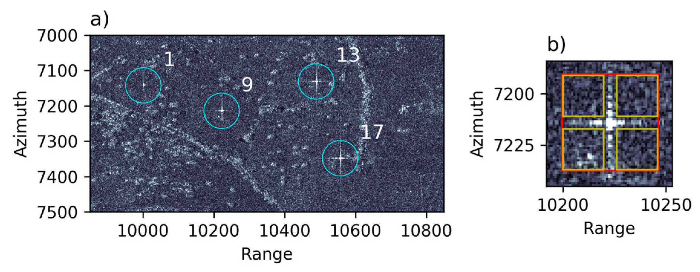
Figure 7.
(a) Extract of a TSX image acquired on 20140120. The impulse responses for four numbered TCR of different sizes are labelled and highlighted by the cyan circles. (b) Zoomed view of the impulse response for TCR 9. The red polygon indicates the ‘target window’ and the yellow polygons indicate the four ‘clutter regions’ used in the point target analysis of each TCR. The part of the ‘target window’ not intersected by the ‘clutter regions’ defines a cross region that encompasses the main lobe and side lobe response of the TCR in range and azimuth directions. TSX data is ©DLR.

Figure 8.
Time series of clutter intensity averaged over the 18 TCR sites in imagery from each SAR sensor. Error bars plot the 2-sigma standard error of the 18 observations for each image. Also plotted in the lower bar chart is the daily rainfall record for Gunning town centre, approximately 3 km away from the TCR array (data obtained from Australian Bureau of Meteorology). The grey polygon indicates a period of relatively stable radar clutter characteristics at Gunning prior to the advent of heavier rainfall events. Image acquisitions falling within this polygon (and indicated in Table 3) are further analysed in terms of RCS, SCR and LOS displacement error in the following sub-sections.

Figure 9.
RCS measurements for each TCR at Gunning. RCS estimates are derived by averaging the values measured in 5 TSX images, 4 CSK images and 3 RSAT-2 images occurring during the period of relatively stable clutter (Figure 8). Error bars are the 2-sigma standard errors of these observations. Theoretical RCS values (Equation (6)) for each TCR size are plotted as dashed lines (X-band) and dotted lines (C-band). Background grey polygons are plotted to aid delineation of the different type groups of TCR design described in Table 2.

Figure 10.
RCS loss due to misalignment of the TCR from the optimum boresight orientation for each SAR sensor. Misalignments for each TCR are given in Table 2. Each RCS loss is calculated by subtracting the image with misalignment from a previous image without misalignment. The RCS of four ‘control’ TCR (numbers 3, 5, 13 and 16) with no misalignment are used to derive the standard errors for each SAR sensor, which are plotted here as 2-sigma error bars. The CSK measurement for TCR number 5 is discarded from this analysis due to flooding of the TCR as described previously in the text. Background grey polygons are plotted to aid delineation of the different type groups of TCR design described in Table 2.

Figure 11.
Contour map of RCS loss as a function of azimuth and elevation misalignments. A minimum curvature surface is fitted to the 7 RCS loss measurements from Gunning SAR imagery for the 1.5 m TCR with positive-valued misalignments. The positions in parameter space of the observed data are plotted as red stars. Observed data is taken as the mean of the TSX, CSK and RSAT-2 values. Contour interval is 0.1 dBm2 with every 0.5 dBm2 bold and annotated.

Figure 12.
LOS displacement error derived from the SCR measurement for each TCR at Gunning. Each error estimate is derived by averaging the values measured in the five TSX images, four CSK images and three RSAT-2 images highlighted in Figure 8 that correspond to relatively stable clutter characteristics. Error bars are the 2-sigma standard errors of these observations. Background grey polygons are plotted to aid delineation of the different type groups of TCR design described in Table 2.

Figure 13.
Magnitude of 2-sigma standard errors on the estimated LOS displacement errors (plotted as error bars in Figure 12) grouped according to TCR size.
Figure 13.
Magnitude of 2-sigma standard errors on the estimated LOS displacement errors (plotted as error bars in Figure 12) grouped according to TCR size.

Figure 14.
Ratio of theoretical SCR to observed SCR for all TCR deployed at Gunning. Background grey polygons are plotted to aid delineation of the different type groups of TCR design described in Table 2.
Figure 14.
Ratio of theoretical SCR to observed SCR for all TCR deployed at Gunning. Background grey polygons are plotted to aid delineation of the different type groups of TCR design described in Table 2.


Table 1.
Estimates of target RCS and the equivalent triangular trihedral CR required to achieve a LOS displacement error of 0.1 mm for different SAR sensors and imaging modes. Ground range resolution areas are calculated for a 35° local incidence angle using pixel resolution information available from the online sources (retrieved 3 April 2017) listed below the table. Pixel resolutions are for single polarisation SLC products. All calculated values are rounded to one decimal place for clarity.
| Band | Sensor | Image Mode | Pixel Resolution (m) | Ground Range Resolution Area (m2) | Clutter (dB) | Pixel RCS (dBm2) | Required SCR (dB) | Required RCS (dBm2) | Equivalent Triangular Trihedral CR Size (m) | ||
|---|---|---|---|---|---|---|---|---|---|---|---|
| Azimuth | Slant Range | Ground Range | |||||||||
| X (9.65 GHz) | TerraSAR-X 1 | Staring Spotlight | 0.24 | 0.6 | 1.0 | 0.3 | −10 | −16.0 | 25 | 9.0 | 0.2 |
| High Res Spotlight | 1.1 | 1.2 | 2.1 | 2.3 | −10 | −6.4 | 25 | 18.6 | 0.4 | ||
| Stripmap | 3.3 | 1.2 | 2.1 | 6.9 | −10 | −1.6 | 25 | 23.4 | 0.5 | ||
| ScanSAR (4 beam) | 18.5 | 1.2 | 2.1 | 38.7 | −10 | 5.9 | 25 | 30.9 | 0.7 | ||
| COSMO-SkyMed 2 | Spotlight | 1.0 | 1.2 | 2.0 | 2.0 | −10 | −7.0 | 25 | 18.0 | 0.3 | |
| HIMAGE (Stripmap) | 3.0 | 3.5 | 6.0 | 18.1 | −10 | 2.6 | 25 | 27.6 | 0.6 | ||
| Wideregion (ScanSAR) | 16.0 | 8.1 | 14.1 | 225.5 | −10 | 13.5 | 25 | 38.5 | 1.1 | ||
| C (5.41 GHz) | Sentinel-1 3 | Stripmap | 5.0 | 5.0 | 8.7 | 43.6 | −12 | 4.4 | 30 | 34.4 | 1.2 |
| Interferometric Wide Swath | 20.0 | 5.0 | 8.7 | 174.3 | −12 | 10.4 | 30 | 40.4 | 1.7 | ||
| Extra Wide Swath | 40.0 | 20.0 | 34.9 | 1394.8 | −12 | 19.4 | 30 | 49.4 | 2.8 | ||
| RADARSAT-2 4 | Spotlight | 0.8 | 1.6 | 2.8 | 2.2 | −12 | −8.5 | 30 | 21.5 | 0.6 | |
| Ultra-Fine | 2.8 | 1.6 | 2.8 | 7.8 | −12 | −3.1 | 30 | 26.9 | 0.8 | ||
| Multi-Look Fine | 4.6 | 3.1 | 5.4 | 24.9 | −12 | 2.0 | 30 | 32.0 | 1.0 | ||
| Fine | 7.7 | 5.2 | 9.1 | 69.8 | −12 | 6.4 | 30 | 36.4 | 1.3 | ||
| Standard | 7.7 | 9.0 | 15.7 | 120.8 | −12 | 8.8 | 30 | 38.8 | 1.5 | ||
| Wide | 7.7 | 13.5 | 23.5 | 181.2 | −12 | 10.6 | 30 | 40.6 | 1.7 | ||
| L (1.27 GHz) | ALOS-2 5 | Spotlight | 1.0 | 3.0 | 5.2 | 5.2 | −15 | −7.8 | 43 | 35.2 | 2.6 |
| Stripmap Ultra-Fine | 3.0 | 3.0 | 5.2 | 15.7 | −15 | −3.0 | 43 | 40.0 | 3.4 | ||
| High-sensitive | 4.3 | 6.0 | 10.5 | 45.0 | −15 | 1.5 | 43 | 44.5 | 4.4 | ||
| Stripmap Fine | 5.3 | 9.1 | 15.9 | 84.1 | −15 | 4.2 | 43 | 47.2 | 5.2 | ||
| ScanSAR (28 MHz) | 77.7 | 47.5 | 82.8 | 6434.6 | −15 | 23.1 | 43 | 66.1 | 15.3 | ||
1 http://www.intelligence-airbusds.com/files/pmedia/public/r459_9_201408_tsxx-itd-ma-0009_tsx-productguide_i2.00.pdf; 2 http://www.e-geos.it/products/pdf/csk-product%20handbook.pdf; 3 https://sentinel.esa.int/documents/247904/685163/Sentinel-1_User_Handbook; 4 http://mdacorporation.com/docs/default-source/technical-documents/geospatial-services/52-1238_rs2_product_description.pdf?sfvrsn=10; 5 http://en.alos-pasco.com/alos-2/palsar-2/.
Table 2.
Details of the 18 TCRs of six type groups deployed at Gunning. Misalignments of the TCR from the optimum boresight orientation for each SAR sensor were only applied for certain image acquisitions (see Table 3) during a secondary experiment described in the text.
Table 2.
Details of the 18 TCRs of six type groups deployed at Gunning. Misalignments of the TCR from the optimum boresight orientation for each SAR sensor were only applied for certain image acquisitions (see Table 3) during a secondary experiment described in the text.
| TCR Type Group | TCR Size (m) | Plate Finish | Perforations | TCR Number | Misalignment (Degrees) | |
|---|---|---|---|---|---|---|
| Azimuth | Elevation | |||||
| A | 1.0 | Metallic | ☒ | 1 | 20 | 0 |
| 2 | 0 | 20 | ||||
| 3 | 0 | 0 | ||||
| B | 1.5 | Metallic | ☒ | 4 | 0 | −20 |
| 5 | 0 | 0 | ||||
| 6 | 0 | 20 | ||||
| C | 1.5 | Powder-coat | ☒ | 7 | 0 | −10 |
| 8 | 20 | 0 | ||||
| 9 | 20 | 20 | ||||
| D | 1.5 | Metallic | ☑ | 10 | 10 | 10 |
| 11 | 0 | 10 | ||||
| 12 | 10 | 0 | ||||
| E | 2.0 | Metallic | ☒ | 13 | 0 | 0 |
| 14 | 0 | 20 | ||||
| 15 | 20 | 0 | ||||
| F | 2.5 | Metallic | ☒ | 16 | 0 | 0 |
| 17 | 20 | 0 | ||||
| 18 | 0 | 20 | ||||
Table 3.
SAR acquisitions of the Gunning TCR array.
| Acquisition # | Date (UTC) | Time (UTC) | SAR Sensor | TCR Alignment Notes | Stable Clutter Period |
|---|---|---|---|---|---|
| 1 | 15 November 2013 | 19:27:59 | TSX | Before TCR deployment | ☒ |
| 2 | 7 December 2013 | 19:27:59 | TSX | Average; only 1.0 m and 1.5 m reflectors | ☒ |
| 3 | 11 December 2013 | 7:14:35 | CSK-1 | Average; only 1.0 m and 1.5 m reflectors | ☒ |
| 4 | 14 December 2013 | 19:18:48 | RSAT-2 | Average alignment | ☑ |
| 5 | 27 December 2013 | 7:14:31 | CSK-1 | Average alignment | ☑ |
| 6 | 29 December 2013 | 19:27:58 | TSX | Average alignment | ☑ |
| 7 | 7 January 2014 | 19:18:47 | RSAT-2 | Average alignment | ☑ |
| 8 | 9 January 2014 | 19:27:57 | TSX | Average alignment | ☑ |
| 9 | 12 January 2014 | 7:14:23 | CSK-1 | Average alignment | ☑ |
| 10 | 20 January 2014 | 19:27:58 | TSX | TSX | ☑ |
| 11 | 28 January 2014 | 7:14:18 | CSK-1 | CSK | ☑ |
| 12 | 31 January 2014 | 19:27:57 | TSX | RSAT-2 | ☑ |
| 13 | 31 January 2014 | 19:18:49 | RSAT-2 | RSAT-2 | ☑ |
| 15 | 11 February 2014 | 19:27:56 | TSX | TSX | ☑ |
| 16 | 13 February 2014 | 7:14:12 | CSK-1 | CSK | ☑ |
| 17 | 22 February 2014 | 19:27:56 | TSX | TSX but with misalignment | ☒ |
| 18 | 24 February 2014 | 19:18:44 | RSAT-2 | RSAT-2 but with misalignment | ☒ |
| 20 | 5 March 2014 | 19:27:57 | TSX | RISAT-1 * | ☒ |
| 21 | 25 March 2014 | 7:14:00 | CSK-2 | CSK but with misalignment | ☒ |
| 22 | 10 April 2014 | 7:13:59 | CSK-2 | CSK but with misalignment | ☒ |
| 23 | 14 April 2014 | 7:13:57 | CSK-4 | CSK but with misalignment | ☒ |
| 24 | 18 April 2014 | 7:13:57 | CSK-1 | CSK but with misalignment | ☒ |
* Several acquisitions were made by the Indian Space Research Organisation for the purpose of calibration and validation of RISAT-1.
© 2017 by the author. Licensee MDPI, Basel, Switzerland. This article is an open access article distributed under the terms and conditions of the Creative Commons Attribution (CC BY) license (http://creativecommons.org/licenses/by/4.0/).
Share and Cite
MDPI and ACS Style
Garthwaite, M.C. On the Design of Radar Corner Reflectors for Deformation Monitoring in Multi-Frequency InSAR. Remote Sens. 2017, 9, 648. https://0-doi-org.brum.beds.ac.uk/10.3390/rs9070648
AMA Style
Garthwaite MC. On the Design of Radar Corner Reflectors for Deformation Monitoring in Multi-Frequency InSAR. Remote Sensing. 2017; 9(7):648. https://0-doi-org.brum.beds.ac.uk/10.3390/rs9070648
Chicago/Turabian StyleGarthwaite, Matthew C. 2017. "On the Design of Radar Corner Reflectors for Deformation Monitoring in Multi-Frequency InSAR" Remote Sensing 9, no. 7: 648. https://0-doi-org.brum.beds.ac.uk/10.3390/rs9070648
Note that from the first issue of 2016, this journal uses article numbers instead of page numbers. See further details here.