100 Years of Competition between Reduction in Channel Capacity and Streamflow during Floods in the Guadalquivir River (Southern Spain)

Abstract

Reduction in channel capacity can trigger an increase in flood hazard over time. It represents a geomorphic driver that competes against its hydrologic counterpart where streamflow decreases. We show that this situation arose in the Guadalquivir River (Southern Spain) after impoundment. We identify the physical parameters that raised flood hazard in the period 1997–2013 with respect to past years 1910–1996 and quantify their effects by accounting for temporal trends in both streamflow and channel capacity. First, we collect historical hydrological data to lengthen records of extreme flooding events since 1910. Next, inundated areas and grade lines across a 70 km stretch of up to 2 km wide floodplain are delimited from Landsat and TerraSAR-X satellite images of the most recent floods (2009–2013). Flooded areas are also computed using standard two-dimensional Saint-Venant equations. Simulated stages are verified locally and across the whole domain with collected hydrological data and satellite images, respectively. The thoughtful analysis of flooding and geomorphic dynamics over multi-decadal timescales illustrates that non-stationary channel adaptation to river impoundment decreased channel capacity and increased flood hazard. Previous to channel squeezing and pre-vegetation encroachment, river discharges as high as 1450 m³·s⁻¹ (the year 1924) were required to inundate the same areas as the 790 m³·s⁻¹ streamflow for recent floods (the year 2010). We conclude that future projections of one-in-a-century river floods need to include geomorphic drivers as they compete with the reduction of peak discharges under the current climate change scenario.

1. Introduction

The present work aims to analyse the relationship between reduction in channel capacity and increase in flood hazard in one of the most affected rivers by climate change in Europe, i.e., the regulated Guadalquivir River in Southern Spain. The analysis of past changes in flood-prone areas and stage-discharge curve in a well-gauged river since the year 1910 allows us to show that non-stationary channel adaptation to anthropogenic forcing (e.g., river impoundment) is of paramount importance in long-term projections of flood risk. In fact, the unexpected rise in inundated areas in the Upper River Basin during extreme rainfall events in 1997–2013 [1,2] contrast with both observed and projected trends of decrease in precipitation and streamflow [3,4].

A pioneering study across the United States [5] highlights the increase in flood frequency because of reduction in channel capacity. Regional transformation of stream valleys had occurred in North America, from widespread aggradation (base-level rise) upstream of dams for several kilometres as a result of damming and backwater effects [6]. More recent research corroborates the relevance of the hydrogeological component in flood risk analysis over multi-decadal timescales with respect to the climate counterpart [7]. The dominant component in the long-term projection of flood risk is routinely assumed to be climate, which determines the probability of extreme hydrological events and streamflow [4,5]. Saint-Venant equations or simplified versions of shallow water equations are subsequently employed to route projected water discharges through the main channel and floodplain assuming a non-erodible bed [8]. In fact, the preferred method of flood hazard mapping in the application of the Flood Directive 2007/60/EC in Europe adopts the two-dimensional hydraulic modelling [9,10]. Geomorphic processes [11] and anthropogenic alterations of the topography [12] that can both mediate and increase the impacts of extreme events and backwater effects, respectively, are usually neglected.

Climate change studies report on a decrease of observed trends in annual precipitation [13] and an increase in projected changes in heavy daily precipitation events in Southern Spain [3,4]. Less precipitation but more concentrated in heavy rainfall events have developed, with annual precipitation and streamflow reduced by 20% [14]. Floods might be less probable in this situation because of the obvious reason that lower river discharges might have induced shallower flows. Surprisingly, exceptional floods with peak discharges of approximately 2000 m³·s⁻¹ occurred in the Upper Guadalquivir Basin between the years 2009 and 2013 and provoked about 150 M€ insured losses. Similar water discharges during previous wet periods (i.e., 1920–1930 and 1960–1970) did not cause such damage.

To better understand changes in flood hazard over time, we lengthen flood records of rare and extreme fluvial events by combining the following two approaches. First, historical floods are reconstructed using a wide collection of hydrological data [1,15], including lengthy gauge records, paleoflood signatures [16] and documentary evidence [17] of extreme events. Second, satellite imagery and aerial photography during peak flow are incorporated to observe the dynamics of modern floods [18,19]. Combining them with post-event orthophotos and LiDAR (Light Detection and Ranging) elevations, grade lines can be inferred [20]. Paleohydrology is also applied to modern floods, allowing us to compare the accuracy of different approaches.

Lastly, we gain insight into flood dynamics using Computational Fluid Dynamics (CFD). Numerical simulations may account for human-made hydraulic structures (in particular, dams) and geomorphic processes (i.e., reservoir sedimentation, channel infilling and vegetation encroachment). Hence, following our previous works [1,21], simulated flooding areas are computed using the open-source software DassFlow-Hydro 2.0 [22]. The use of remote sensing helps to verify the hydraulic reconstruction of modern floods across a lengthy 70 km stretch of up to 2 km wide floodplain, while paleohydrological data benchmark local points of interest. Note that the comparison of paleohydrological records, remote sensing data and hydraulic modelling are not part of standard risk analysis, but are an original method of study proposed in this paper. Furthermore, the combination of the three methods serves to identify hydrogeological drivers of flood hazard.

The paper is organised as follows. Section 2 presents a brief description of the study site and recaps material and methods (some of them used in our earlier publications [1,21,23]). Section 3 presents a detailed study of modern floods by combining remote sensing data based on satellite images and helicopter flood photography with model simulations. Section 4 discusses the relation between the observed increase in flood impacts and the decrease in channel capacity at flood stage over time in the Guadalquivir River. Finally, Section 5 outlines our conclusions.

2. Materials and Methods

2.1. Study Site

The field area is situated along a stretch of the Guadalquivir Valley in Southern Spain, upstream of the border of the provinces of Jaén and Córdoba (Figure 1). The fluvial regime is typically Mediterranean, showing a summer drought period with minimum water levels and highest values in winter and spring. The complex topography of the surrounding landscapes, the large size of the drainage area (19,546 km²) and the different climate influences of the Mediterranean Sea and the Atlantic Ocean favour the occurrence of heavy precipitation events and floods [24]. Indeed, flooding is the most damaging type of natural disaster in this area with economic losses per province ranging between 200 × 10⁶ and 1200 × 10⁶ € [25].

The selected river reach is of 70 km length and 170 m bankfull width. The river flows across two confined valleys at the inflow and outflow boundaries. Between the confined valleys, 45 km of meanders with 5–6 m bankfull depth were sculpted in the lower sand-mud terrace. The incised meandering channel formed unpaired terraces across its floodplain, intensively used by the human activity. Several farms and villages, one town (i.e., Villanueva de la Reina) and one city (i.e., Andujar) are vulnerable to floods, as depicted in Figure 1. Indeed, characteristic flow depths during large floods are larger than 6 m in the meandering floodplain and 10 m in the confined valleys [1]. Inundated areas in the meandering reach, where urban areas and irrigated crops are usually submerged, are about 2 km wide during exceptional hydrological events.

The mean bed slope in the meandering stretch is 0.072%, lower than the original value of 0.12% for a straight channel configuration. The adaptation of bed slope to downstream valley slope (0.076%) indicates the existence of a downstream hydraulic control of meander dynamics by the confined valley in Marmolejo [26]. The bed substrate is made of clasts and rounded coarse gravels with grain diameters in the range of 6–40 cm except in the downstream valley, where slate outcrop is exposed if transport capacity exceeds sediment supply. Meanders are stable as they did not migrate even during the past wet periods (1920–1930 and 1960–1970) when the peak river discharges reached values between 1400 and 3000 m³·s⁻¹ [1]. Appendix A gives stable meander dimensions.

To conclude, it is worth noting the presence of four dams distributed along the studied river reach (Figure 1). As we shall see, they play a key role in the dynamics of floods. The four hydropower stations referred to as Mengíbar, San Rafael, Valtodano and Marmolejo dams work since 1916, 1912, 1919 and 1910, and have maximum heights of 12, 5, 6 and 20 m, respectively. Mengibar dam is characterised by adjustable floodgates that prevent reservoir sedimentation. Conversely, Marmolejo dam uses tainter gates and spillways elevated 12 m above the outlet channel. The absence of bottom withdrawal spillways in Marmolejo dam provoked a 70% silting degree of the reservoir and the colonisation of mud by riparian vegetation [1]. In fact, the tail of the silted-up reservoir extends 15 km upstream of Marmolejo dam, up to the Roman Bridge of Andújar (see Section 3).

2.2. Gauging Records, Documentary, Imagery, Sedimentary and Botanical High Watermarks

Here, we adopt the same approach as in previous publication. As methods have been detailed previously and at length in [1], we will not dwell in depth on this issue. However, a summary explanation is needed.

Systematic measurements of river discharge and flow depth at hydropower and gauge stations are publicly available in Spain [27,28]. The earliest record dates back to 1910 at Marmolejo dam. The selected study site includes two additional hydropower stations with gauged data, namely: Mengíbar and Valtodano. Rare and extreme floods typically prevented in situ measurement of peak water discharge at these locations because stages were deep enough to overtop stations vigorously [16]. In fact, overtopping of station happened during several flood episodes (e.g., the 1924, 1963 and 2010). To lengthen flood records of such rare and extreme fluvial events, we used documentary information from the National Database of Historical Floods [29] (freely accessible on-line [30]).

Furthermore, we compiled additional records based on in situ photography of floods (e.g., Figure 1). Aerial photography acquired from a helicopter by the Civil Protection Services in Andalusia are available on 23 and 24 February 2010 between 15:00 and 16:00 and 10:00 and 11:00, respectively. It is worth noting that this is an accurate source of information regarding the most catastrophic flood event because it captured the inundation at peak flow. Upstream of the meandering floodplain and downstream of Andújar city the peak water discharge achieved 1070 and 1928 m³·s⁻¹ (

Table 1. Peak river discharges at Mengíbar (inlet) and Marmolejo (outlet) dams in February 2010, December 2010 and April 2013 floods.

Event	Peak Flow
No.	Location	Date and Time	Q Local (m3·s−1)
1	Inlet	23 February 2010 18:00	1070
1	Outlet	24 February 2010 11:00	1928
2	Inlet	08 December 2010 09:00	648
2	Outlet	09 December 2010 09:00	1433
3	Inlet	02 April 2013 03:00	671
3	Outlet	02 April 2013 16:00	1378

), respectively. Using these images, or combining them with Landsat/TerraSAR-X satellite images, we delimited the inundation extent shown in Figure 1 that serves to verify the numerical model results in Section 3. Additionally, a catalogue of imagery (KMZ format) containing flooded areas on 8 December 2010 is also available.

Historical cartography [31,32] and sequence of orthophotos [33] depict the evolution of the channel planform since 1883 and 1956, respectively. Historical maps are available in 1900, 1924, 1938 and 1989 across the study area [32]. In addition, local maps at specific locations subject to water management exist in 1879, 1883, 1889, 1902, 1918 and 1940 [31]. Orthophotos in the Upper Guadalquivir Basin correspond with the years 1945, 1956, 1977, 1984, 1997, 2001, 2004, 2007, 2009, 2011 and 2013 [33]. Combining historical cartography and orthophotos, we were able to identify the meander with the largest migration rate as well as the most aggraded straight channel. Furthermore, the orthophoto of the year 2013 was particularly useful because it depicts the most elevated slackwater deposits along the riversides after the most recent flood (April 2013), which was of similar magnitude than December 2010 event (see Table 1). It allowed the identification of high water marks and paleostage indicators (HWM-PSIs) and the delimitation of the inundated area in the confined valley setting. As a matter of fact, the 0.5 m spatial resolution of the 2013 post-event orthophoto was much better than the 30 m resolution of TerraSAR-X and Landsat images. Satellite images could not be used in the upstream and downstream confined valleys of 150–200 m bankfull width, as explained in Section 3.3.

Lastly, post-event fieldworks were conducted between October 2015 and April 2017 to survey high watermarks from historical images, shoreline elevation of modern floods from aerial photography, mud lines on bridge piers, overbank flood-deposited sediments and botanical records (e.g., scars on trunks and woody debris). We employed a modern Leica Zeno 20 Global Positioning System (GPS) combined with laser Leica DISTO^TM to locate inaccessible stage indicators. Subsequently, correlating the date and time of flood record with inferred flood stage and river discharge yield the rating curve.

2.3. Satellite Imagery: Landsat-5 and TerraSAR-X

Landsat-5 Thematic Mapper (TM) image of flooding on 24 February and 9 December 2010, at peak streamflows in Marmolejo dam of 1928 and 1412 m³·s⁻¹, respectively, were downloaded from the USGS through EarthExplorer^TM at WRS-2 Path/Row 200/34 (

Table 2. The Landsat and TerraSAR-X imageries used in this study.

River Reach	Event	The Available Satellite Images
	No.	Source	Date and Time	Q Outlet (m3·s−1)	Q Inlet (m3·s−1)
10–59 km	1	Landsat	24 February 2010 11:40	1882	1024
30–70 km	1	TerraSAR-X	05 March 2010 18:06	653	321
0–52 km	2	Landsat	09 December 2010 11:39	1412	350
0–70 km	2	TerraSAR-X	09 December 2010	1095	309

). We acquired the level 1 terrain (L1T) corrected product that is radiometrically and geometrically processed and includes correction for relief displacement [18,34]. Subsequently, these images were processed with ArcMap 10.3 (Esri: Redlands, CA, USA), using the 5-4-3 (SWIR, NIR, Red) band combination that permits to highlight the water surfaces. The length of the spatial extent that Landsat images partially wreathe is given in Table 2.

In addition, TerraSAR-X radar satellite images were used to identify inundated areas in non-visible regions covered by clouds in Landsat due to spectral behaviour (Table 2). Such data were acquired and processed by the local government of Andalusia and is available through REDIAM [33]. Detailed features of TerraSAR-X image are as follows: 29.5°–32.4° incidence angle, StripMap (50 × 30 km; 3 m) image mode, HH polarisation, MGD-ORISAR 2 m product type and geometrically optimised resolution. In this process, the images were geometrically and radiometrically optimised with the object of extracting the flood mask. This extraction was based on the characteristic spectral signature of the water sheet over terrestrial zones that allow identifying with accuracy the margins of the same. Taking into account that the characteristic spatial resolution of scenes was 30 m, with mean geodetic accuracy lower than one-quarter of a pixel, flooded areas in the 45 km stretch of up to 2 km wide meandering floodplain could be readily mapped. Remote sensing derived water stages were obtained on the observed shorelines from post-event LiDAR elevations [35] (spatial resolution ≤1.4 m). We located the observation points where terrain slope vanishes. In doing so, root-mean-square (RMS) and maximum errors in inferred stage should approach LiDAR errors lower than 0.2 m and 0.4 m, respectively.

By comparing the river discharges of the satellite images (Table 2) and the peak streamflows at the inlet and outlet river reaches (Table 1), we conclude that available remotely sensed images capture the peak flood event in some sub-region but not in the entire domain. Hence, we selected spot locations at the optimal region-growing output to infer image-based water levels wherever appropriate. We integrated water levels from the satellite images with flood model via validation. Furthermore, the comparison of remote sensing stage with the rest of evidence serves to show the accuracy of this technique.

2.4. Two-Dimensional Shallow Water Numerical Simulation

Following our previous works [1,21,23], the 2D unsteady shallow-water model implemented in the open-source code Dassflow-Hydro 2.0 [22] was used to simulate flooding areas, maps of water flow depth and two-dimensional velocity vectors. It is the preferred method of flood hazard mapping in the application of the Flood Directive 2007/60/EC in Europe [9,10]. Anthropogenic alterations of the topography, backwater effects, hydraulic jumps, backflood of tributary and wet/dry fronts can be computed with success using this approach [12].

The extent of the computational domain was chosen from Mengibar dam (inlet) to the floodplain 6 km downstream of Marmolejo dam (outlet) shown in Figure 1. In doing so, we avoided the influence of the boundary conditions on the numerical results at the meandering river reach [36]. The computational mesh was obtained by patching a 5 m resolution digital elevation model [35] with the channel and reservoir bathymetry (obtained from SONAR measurements) and the dam/spillways geometry (measured in situ with the Zeno 20 GPS + Leica DISTO^TM S910, Heerbrug, St. Gallen, Switzerland). We set the cell size and their distribution in the computational grid to ensure the mesh of the channel, reservoirs, dams and spillway piers replicate reality.

The cell size of the computational mesh was thinner than 1 m near hydraulic structures. Far from infrastructures, the computational grid was coarser with characteristic edge lengths of 5 m in the channel and 10 m in the floodplain. Consequently, a minimum of 30 cells was uniformly distributed along the bankfull channel cross section of 150 m characteristic width, 150 cells defined the 1.5 km wide cross section of an inundated meander, and about 200 cells were used in the tainter gates over the spillways of Marmolejo dam. These spatial resolutions led to mesh with 2.5 million triangular cells. The model captures backwater effects intrinsically in river flows through sudden channel contractions and over-elevated spillways without needing to prescribe internal boundary conditions thanks to the trustworthy geometry of the computational mesh. Furthermore, the use of the river bathymetry allowed us to account for the base-level rise in a severely aggraded river stretch.

We set Manning’s roughness coefficient in the 2D flood model to 0.04, 0.06, 0.12 and 0.26 s·m^−1/3 in arable crops, the channel, sparse and dense forest corresponding to a depth of flow reaching branches, respectively [37]. Numerical simulations run without parameter tuning. We addressed the accuracy of the numerical results by comparing the simulated stage with helicopter image-based water levels, remote sensing data, HWM-PSIs and systematic gauge records at peak flow (Section 3).

We forced a steady state regime in the model by setting the peak streamflow as inflow boundary condition both at the main river and regulated tributaries. Hourly-average discharges measured in the main channel (Mengíbar and Marmolejo dams) as well as in the Rumblar and Jándula tributaries (Zocueca and Encinarejo dams, respectively) served to check the validity of the steady-state hypothesis at peak flow. Figure 2 shows the unsteady hydrograph in these gauge stations. Assuming a quasi-steady regime and using the continuity equation of the water phase, we evaluated the water discharge at the outlet as the sum of the inflow contributions (blue line in Figure 2). The computed outflow discharge was 1899 m³·s⁻¹ while the measured value was 1928 m³·s⁻¹. Thus, the relative error was 1.8%. This small difference implies that peaks in the tributaries occurred nearly at the same time/day as in the outlet boundary location of the main channel. Taking into account that the flow regime in the Guadalquivir River is quasi-steady during floods, the numerical modelling was notoriously simplified. The numerical simulation was run until the flood wave inundated the whole channel, attaining a steady state at late time.

3. Results

3.1. Maximum Stage Profile in Modern Floods

To visualise the spatial dynamics of the flood wave and address the accuracy of the model prediction in each sub-region, Figure 3 shows bed elevation, simulated and measured water levels against distance to Mengíbar dam at peak flow on February 2010. The presentation of model results is based only on flood stage (this section) and inundation extent (forthcoming sections) because of the obvious reason that satellite and helicopter imagery, among other evidence, do not provide values of flow velocity vectors, though numerical simulation does.

Along the first 45 km, the flow depth was quasi-uniform, and the water surface profile was nearly parallel to the thalweg profile. This sub-region comprises the inlet confined valley, including the first two dams (i.e., Mengíbar and San Rafael), and a large portion of the meandering river reach crossing the town (i.e., Villanueva de la Reina) and the third dam (i.e., Valtodano). The flood overtopped the second and the third dams (i.e., San Rafael and Valtodano). Further downstream, at a distance of 47.5 km and near the city (Andújar), a nick point developed due to reservoir sedimentation, delta formation and channel infilling. Aggradational wedges of fine-grained sediment inside Marmolejo reservoir (47.5–64.3 km) were trapped after dam construction (in 1962) provoking a decrease in bed slope from 0.072% (original value) to zero (present value). Note that the largest change in slope indeed occurs between the city and the farms, where bed slope vanishes. The water surface profile also reflects this phenomenon because the hydraulic grade line is horizontal between the city and the farms. Next, the free surface slope suddenly increased when water entered into the outlet confined valley. The bed slope also retrieved the basin slope there. Lastly, downstream of Marmolejo dam, the flow was quasi-uniform similar to the inlet confined valley.

Overall, simulated stages agree with inferred values from Lansat 5 image (circles in Figure 3), aerial photographs from a helicopter (squares) and stream gauges (diamonds). Interestingly, water levels from satellite and photography overlap each other, showing the accuracy of both methods. Next, we detail the precise values of the stage shown in the graph.

Table 3. Mean water level and RMSE in the numerical flood simulation using selected spot locations. The data source used to evaluate RMSE correspond with the following order of confidence: gauge station, in situ imagery, remote sensing data and PSI. All data are in metres.

Location	Simulation	Satellite	Imagery	Gauge	PSI	RMSE
Outlet Valley	185.6	-	185.7	-	185.7	0.1
Outlet Reservoir	190.9	-	-	190.4	-	0.5
Farms	197.7	196.8	197.2	-	-	0.5
Village	197.9	197.0	197.5	-	-	0.4
City (Bridge)	198.9	-	199.3	198.8	-	0.1
City (Highway)	201.1	201.5	200.9	-	-	0.2
Valtodano	[210.8, 206]	[205.4, 210]	-	-	-	0.6
	206.3	-	206.2	-	-	0.1
Town	[214.9, 221]	[215, 219.5]	-	-	-	0.7
	215.8	-	216	-	-	0.2
	217.6	217	-	-	217.7	0.6
Inlet Valley	237.5	-	238.2	238	238.2	0.5

shows the specific values of simulated water levels at carefully selected spot locations with near flat topographic gradient, away from edge of buildings and with no or very short vegetation. Root Mean Square Error (RMSE) in simulated altitude with respect to evidence is also given. Along the outlet valley axis, simulation, in situ photography and HWM-PSI are in excellent agreement with RMSE = 0.1 m. The inferred elevation from flood photograph coincides with the field evidence. Few metres upstream, in the reservoir of Marmolejo dam, RMSE was evaluated with the systematic gauged record and raised up to 0.5 m. In the farms, 6 km upstream of the dam, we obtain the same RMSE as in the reservoir. Satellite images underpredict the maximum stage from helicopter photographs at peak flow by 0.4 m at this location. The main sources of error in remote sensing data are the clouds affecting Landsat images and the TerraSAR-X lag time of 9 days. Results in the village are similar. The existence of a gauge station in the Roman Bridge of Andújar city allows us to evaluate with accuracy the model prediction error nearby larger urban areas. There, the simulation overpredicts the water level only by 0.1 m. The use of photographs acquired from helicopter overpredicts the water elevation by 0.5 m. We attribute this disparity to the accuracy of the LiDAR elevation data with RMS error in the range of 0.2–0.4 m in the inundated riparian forest where we infer the stage.

In the meandering floodplain, which encloses Valtodano dam and the town, RMSE between simulated and satellite image-based water level is lower than 0.7 m. The agreement is even better between simulation and in situ photography, with RMSE ≤ 0.2 m. Lastly, along the narrow, confined valley at the inlet of the study site, satellite images could not be used. We adopted the gauged record as true value to compute the error. On the one hand, imagery and HWM-PSI provides a similar elevation which is 0.2 m higher than the true value. On the other hand, the numerical simulation underpredicts by 0.7 m the stage. Regarding simulated flow depths, we found out maximum values deeper than 10 m at the inlet and outlet confined valleys, in agreement with gauged records. In the meandering river reach, the flow was shallower and simulated flow depths typically varied in the range of 7–8 m.

3.2. Verification of Inundated Areas in a Meandering Floodplain

In this section, we evaluate the spatial accuracy of the model simulation in terms of inundation extent by comparing with remote sensing data from Landsat on 24 February 2010 at 11:40. The observed shoreline was corrected where clouds exist (white smudges in Figure 4a) using in situ photography of the flood at 11:45. At this time, the river discharge was 1024 and 1882 m³·s⁻¹ at the inlet and outlet of the study site (Table 2), which approaches the peak value of 1070 and 1928 m³·s⁻¹ (Table 1). Figure 4a shows the original satellite image and the delimited inundation extent.

Figure 4b depicts the simulated elevation of the water surface (contour map) and the observed wet perimeter (solid line in black). Simulated flooded areas overlap observed ones in the meanders between the town and Valtodano dam, but some discrepancies appear due to the presence of islands in the numerical simulation and the small overflooded area near Valtodano dam. Solid lines in blue split the classified elevations into steps of 1 m depth. The shape of the isocontours is complex across the area. This fact commonly characterises two-dimensional flows because in the simple case of one-dimensional flows the isoelevations are simply perpendicular to the mean streamflow direction.

Scarce stage indicators exist in this region as a consequence of the intensive human activity that destroyed most evidence in arable crops over the floodplain. Exceptional paleostage indicators were identified in the meander with the highest sinuosity (Figure 4b). Modern floods (years 2009–2013) provoked depositional PSIs as woody debris and slackwater deposits (Figure 4c,d). In addition, channel-scale concave sculpted forms were found in the outer floodplain of the channel bend [38]. These puzzle erosional bedforms resemble plunge pools in loose granular material [39]. They are found at the back of a 2.5 m height bump over the riverbank and made of depositional sequences of laminated fine sand and dunes. Erosional forms lead us to think that the wake flow of the bump developed whirlpool vortex and formed plunge pools during modern floods. The 217.7 m elevation of field evidence corroborates the simulated water stage of 217.6 m (see Table 3).

Finally, we focus on the accuracy of the simulation regarding inundation extent (

Table 4. Comparison of inundation extents from model simulation and remote sensing data.

River Reach	Data Source	Aobs (km2)	Amod (km2)	${\mathit{A}}_{\mathit{obs}} {\displaystyle \cap } {\mathit{A}}_{\mathit{mod}}$	CSI
Inlet valley	Photography	0.580	0.528	0.461	0.81
Meandering stretch	Satellite + photos	10.303	10.937	9.408	0.80
Farms-city floodplain	Satellite + photos	16.279	15.761	14.516	0.83
Outlet valley	Photography	1.911	1.941	1.755	0.84

) as errors in water levels has been already presented in Section 3.1 at the observation spots (Table 3).

To this end, we adopt the same quality index as proposed in the pioneering work by Bates and De Ro [40], referred to as critical success index (CSI):

$$CSI=\frac{A_{obs} {\displaystyle \cap } A_{mod}}{A_{obs} {\displaystyle \cup } A_{mod}}$$

(1)

where A_obs and A_mod represent the sets of pixels observed to be inundated and predicted as inundated, respectively. CSI equals 1 when simulated and observed areas coincide exactly, and equals 0 when no overlap exists. Table 4 shows a summary of results in the different river reaches where we applied this method. In the meandering stretch, the CSI or F-statistic is 0.8. According to previous flood simulation studies, there are a relatively small number of simulations with CSI > 0.7 [41,42]. Hence, we conclude that the model simulated inundation extent is reasonably good with respect to the remote sensing data.

3.3. Flood Maps in a Confined Valley Setting

In the confined valley downstream of Mengíbar dam, which represents the inlet river reach of the study site, the maximum stage measured in the gauge station in February 2010, December 2010 and April 2013 were 237.7, 238.4 and 237.3 m for streamflows of 671, 1070 and 648 m³·s⁻¹ (Figure 5a). The corresponding bankfull width at the site (second bridge in Figure 5b) was 125, 139.2 and 118 m and the flow depth achieved 9.7, 10.4 and 9.3 m, respectively. The bankfull width increased only by 18% (i.e., 21 m) when the water discharge grew from 650 to 1050 m³·s⁻¹. Hence, the narrow channel prevents from using the 30 m resolution satellite images in the verification stage of the simulation.

Alternatively, we delimited the inundation extent from visible shorelines in helicopter photographs on 24 February 2010 14:45 with 1024 m³·s⁻¹. Another data source that is particularly useful to verify the model in the confined valley is the high-water mark (e.g., the mud-line on bridge pier), as it records nearly the same stage as the gauge (Table 3) with an error in flow depth of 2% (i.e., 0.2 m). Furthermore, overbank flood-deposited sediments are visible in the April 2013 post-event orthophoto along the riversides and over areas where velocity magnitude suddenly decreased.

The perimeter in red in Figure 6a represents fine slackwater deposits along the channel margin. Three fully silted reservoirs located 45 km upstream favoured the high sediment supply because they could not retain sediments during the 2010–2013 floods and, consequently, much sediment was supplied to the Guadalquivir River. The flood wave transported and deposited fine-grained sediments that are widespread in the channel. Laterally-attached sandy siltlines in the natural channel bend (red line) overlap with the simulated inundation extent (blue line). The observed water level from flood photograph (black line) is in agreement with the simulation and sedimentological evidence in the outer riverbank. The quality index of the simulated inundation extent is CSI = 0.81 (Table 4), which supports our numerical results. Interestingly, the area enclosed by slackwater sediments (i.e., 0.218 km²) represents the 47% of $A_{obs} {\displaystyle \cap } A_{mod}$ and extends along the 80% length of the analysed stretch, showing that paleohydrology can contribute to reconstruct modern floods in places where remote sensing data are not accessible.

The computed map of depth-averaged velocity magnitude (Figure 6b) indicates that laterally-attached sandy siltlines emplaced from suspension occurred where flow boundaries reduced local velocities relative to the mean channel velocity. The velocity magnitude downstream of the bridge was typically in the range of 1.5–2 m·s⁻¹ along the thalweg and increased up to 3–5 m·s⁻¹ at the natural channel bend and a flow contraction area. Slower flows with velocity below 1.5 m·s⁻¹ occurred in the vegetated island between the two bridges, the inner side of the bend and the top of the riverbanks, in agreement with visible slackwater flood deposits. This phenomenon contributed to bar formation at natural channel bend. Regarding the contours of water surface elevation, we found them aligned with the cross section of the channel and perpendicular to the streamwise direction in this occasion (Figure 6c). This pattern corresponds with a uni-directional flow. The surface slope vanishes between the bridges, increases at the bend due to local head losses and retrieves the thalweg slope, as shown in Figure 3 with distances to the dam lower than 3.5 km.

Lastly, we briefly describe the main characteristics of the flood in the confined valley at the outlet of the study site (Figure 7). We refer the reader to our earlier publication [1] for a detailed analysis of available flood records and their good correlation with numerical results. In fact, CSI achieves the value of 0.84, which represents a maximum on the rest of river reaches.

When water enters into the valley, it feels the presence of Marmolejo dam. We observe that the surface elevation decreases progressively from 198.5 to 195.5 m along the first 3 km. Then, in less than 1.5 km, altitude suddenly decreases to 190.3 m in the flow over the spillways. Water sharply falls at the foot of the dam, reaching an elevation of 186 m. Downstream of the dam, the natural river flow is unaltered, and the water surface adopts the channel bottom slope. As it happens in the other confined valley, water levels of constant altitudes are perpendicular to the main flow direction and, consequently, the flow is quasi-unidirectional.

The one-dimensional representation of the water level as a function of the streamwise distance, recall Figure 3, makes easier the visualisation of the effects of Marmolejo dam on the flow behaviour. The area in Figure 7 corresponds to the streamwise distance range of 60–70 km in Figure 3. There are two factors increasing the water level upstream of dam: first, the 12 m high dam by itself; second, the silted-up reservoir that increases the base level and decreases the channel bottom slope (0.06%) with respect to the original valley slope (0.076%).

We verified the simulated stage with gauge data at the reservoir and foot of the dam at peak flow in February 2010 flood (see Figure 8a). The simulated rating curve (dashed line) matches the observed one with the peak river discharge Q = 1928 m³·s⁻¹ and an elevation of 190.3 m. In addition, the simulation predicts the 186 m observed stage with an absolute error of 0.2 m when Manning’s roughness is 0.06 s·m^−1/3. Consequently, the numerical simulation can reproduce with accuracy the flow over the spillways, even in the presence of an over-elevation of 4.3 m between the stages upstream and downstream of the dam. To quantify the over-elevation in the wide range of streamflow Q ≤ 3000 m³·s⁻¹, we conducted additional numerical simulations, as shown in Figure 8a. In practice, the 12 m high Marmolejo dam heightens the water level by 6.9, 5.2, 4.3, 3.7 and 3.2 m for 1000, 1500, 2000, 2500 and 3000 m³·s⁻¹. Unfortunately, such increases in flow depth propagate upstream when the flow regime is subcritical, as it happens in our case.

3.4. Backwater Effect Upstream of Dam and Silted-Up Reservoir

To benchmark the accuracy of the numerical simulation against systematic instrumental data for river discharges provoking floods in the floodplains of Andújar city, Figure 8b depicts the simulated elevation of the water surface as a function of the river discharge at the stream gauge below the Roman bridge. The distance to Marmolejo dam is 15 km (see also the sketch in Figure 3). The observed stage for 1400 ≤ Q ≤ 2000 m³·s⁻¹ varies between 197.9 and 198.8 m, while the simulated values are 198.2 and 198.5 m, respectively. Taking into account that the thalweg is 190.0 m, the measured (computed) depths are 7.9 (8.2) and 8.8 (8.5) m. The agreement between simulated stage and gauged record is good because absolute and relative errors are lower than 0.3 m and 3.8% for Q ≥ 1400 m³·s⁻¹. The experimental data show some hysteresis while the numerical simulation provides a one to one relation between stage and discharge. However, differences are small during floods.

Several points emerge from the analysis of the inundated extent downstream of Andújar city (Figure 9). We delimited the observed inundation extent as in Section 3.2. The model simulation extent is reasonably good with respect to the remote sensing data and achieves the quality index of CSI = 0.83 (Table 4). The width of the flooded area reaches a maximum of 2.2 km just behind the outlet confined valley. This value doubles the 1 km flood-prone width in the meandering stretch (Figure 4). Second, flood impacts are higher than expected from historical records. For instance, the National Database of Historical Floods [29,30] establishes that the village and the city were inundated uniquely in the previous years 1963 and 1945 with river discharges in the range of 2500–3000 m³·s⁻¹. Taking into account that the peak river discharge was 1928 m³·s⁻¹ in February 2010, we conclude that flood risk has increased over multi-decadal time scales in the Guadalquivir River.

Anthropogenic alterations of topography due to the construction of a 12 m high dam in the outlet confined valley (i.e., Marmolejo dam) increased the impacts of extreme events due to backwater effects. The direction of the flood wave in the southern floodplain was opposed to the direction of the flow in the main channel due to the flow contraction regime when approaching the downstream confined valley setting. We do not show the details of flow velocity for the sake of brevity. The over-elevation in Marmolejo dam amplifies this effect (recall Figure 8a). This phenomenon is referred to as backwater effect in the hydraulic literature and typically occurs at subcritical speeds in the presence of hydraulic structures [12], as in the present case. Another contribution to increasing flood hazard is reservoir sedimentation. Recall that Figure 3 depicts the tail of the silted-up reservoir reaching the Roman bridge of Andújar. The aggradation and base-level rise extend upstream of the dam for 16.8 km, where the water surface elevation suffers a similar effect (see stages along 47.5–64.3 km in Figure 3).

4. Discussion: Effects between Streamflow and Channel Capacity

4.1. Trend in Streamflow over Time

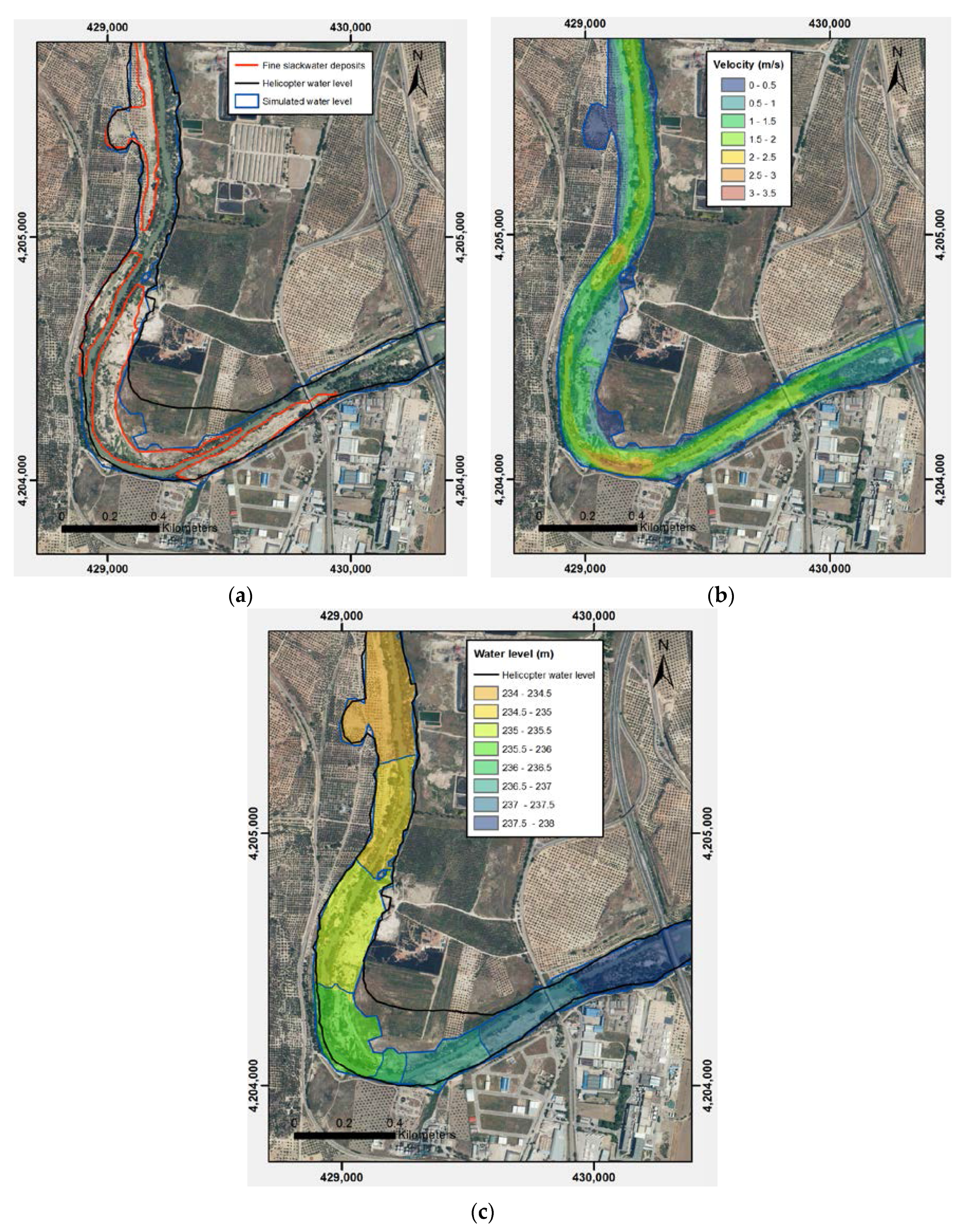
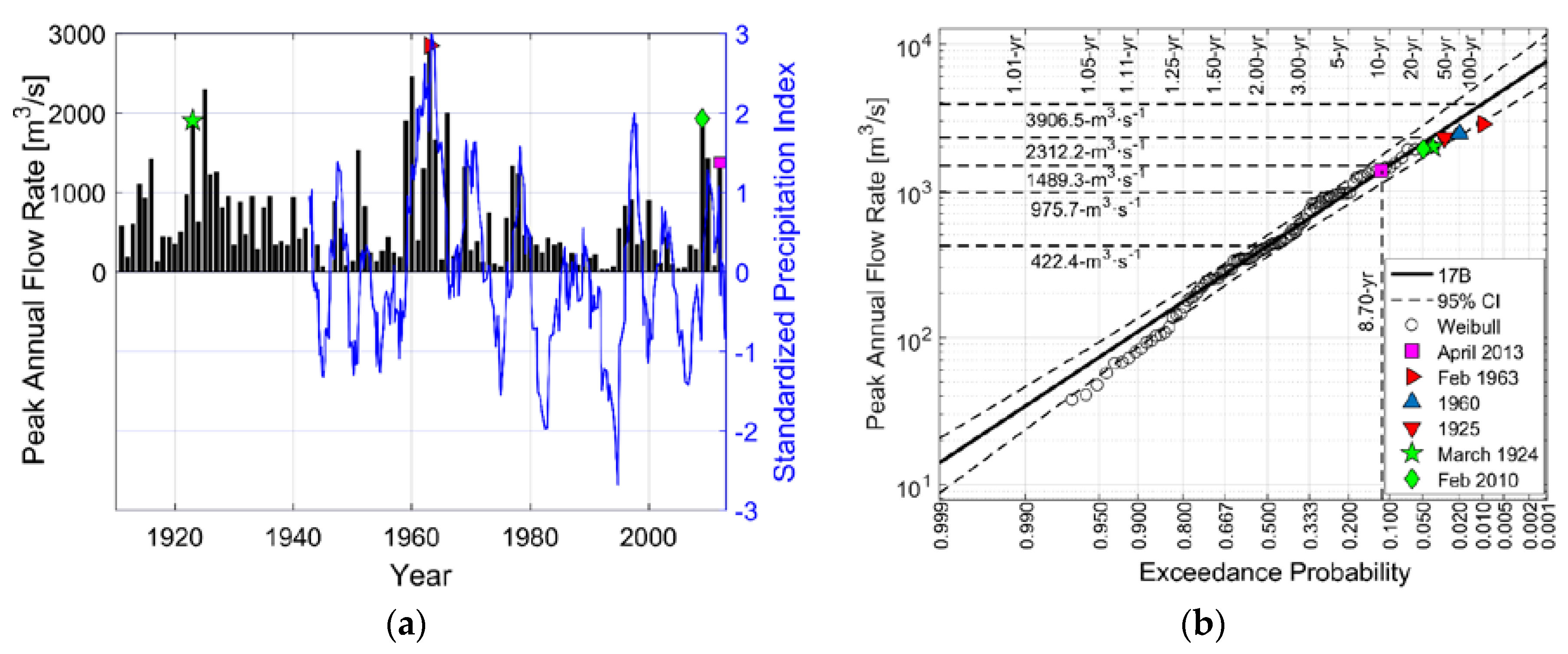
Figure 10a shows maximum annual river discharge values at the study site aiming to provide an idea of the severity and frequency of flooding since the year 1910. Climatically, the first half of the twentieth century registered periods of high flood recurrence (1910–1930) with discharges on the order of 1000–2300 m³·s⁻¹, but also of moderate events (1930–1950) lower than 1000 m³·s⁻¹. Unusually high flood frequencies occurred in the period 1951–1980. The most catastrophic flood developed in winter of 1963 with a peak water discharge as high as 2850 m³·s⁻¹. Persistently drier conditions with scarce hydrological events were observed between 1980 and 1996. In the 21st century, flood frequency and magnitude decrease, with peak annual flow rates of approximately 1300–2000 m³·s⁻¹ in the period 2009–2013. Since then, we are suffering a period of drought. Subsequently, the recurrence intervals of maximum flood magnitudes were evaluated using the Bulletin 17B and Expected Moments Algorithm procedures implemented in PeakFQ [43]. Figure 10b shows the exceedance probabilities and return periods of both systematic and historical (high outliers) floods. Floods highlighted with a green pentagram, and diamond symbols correspond with March 1924 and February 2010 extreme events, respectively, and an associated return period of about 20 years. Rare hydrological events with larger return periods occurred in 1960 (50 years) and 1963 (100 years).

It is worth proving that the observed decrease in peak streamflows in the post-impoundment era (i.e., since approximately 1950) is due to less frequent precipitation in the Guadalquivir River Basin, as established in climate change reports [3,4]. The climate component shows the decrease in time of the annual precipitation across the Guadalquivir Basin [13,14]. Here, we adopt the standardised precipitation index (SPI), which is based on a proper statistical distribution of the precipitation [44]. Originally, it was developed for drought detection. Later, it was used with success as a regional system for climate risk monitoring and to detect the potential threat of possible flood events.

Figure 10a compares the peak annual streamflow and the 36 months SPI curve. Interestingly, we got positive values of SPI during the periods of high flood recurrence commented beforehand. The largest value of 3.01 occurs in the hydrological year 1963 when the largest flood occurred. Other local maximums, with SPI values of 1.63, 1.57, 1.99 and 1.28, are well correlated with extreme floods in 1970, 1979, 1997 and 2010. Interestingly, reservoirs attenuated the hydrological event of 1996 because of their nearly empty states after the drought period 1980–1996, when SPI reached −2.68 (values lower than −1.65 correspond to extreme drought [45]). Unfortunately, all the reservoirs attained the top water level in the rest of extreme rainfall events, and could not regulate the peak streamflow.

4.2. Effects of Vegetation Encroachment and Aggradation on Channel Capacity

The term channel capacity has two senses according with the existing literature: originally, it represents the cross-sectional channel area at flood stage A_FS [46,47]; a broader meaning refers to the average cross-sectional discharge at flood stage Q_FS which is evaluated as the product of A_FS and the cross-sectional average flow velocity V_FS [5,48]. In the first case, the unique cause of changes in channel capacity can be bed aggradation/degradation or channel narrowing/widening. In the second case, channel capacity can be controlled not only by depth and width at flood stage but also bed slope and boundary roughness (e.g., grain size and bank vegetation). Hence, we refer to channel capacity at flood stage as the volume of flow that can be carried within the channel at flood stage Q_FS. To close the concept, we define the flood stage as an established gauge height for a given location above which a rise in water surface level begins to create a hazard [5]. We identified it with the bankfull stage from the proto-floodplain (top of the point bar surface) that supports woody vegetation [49].

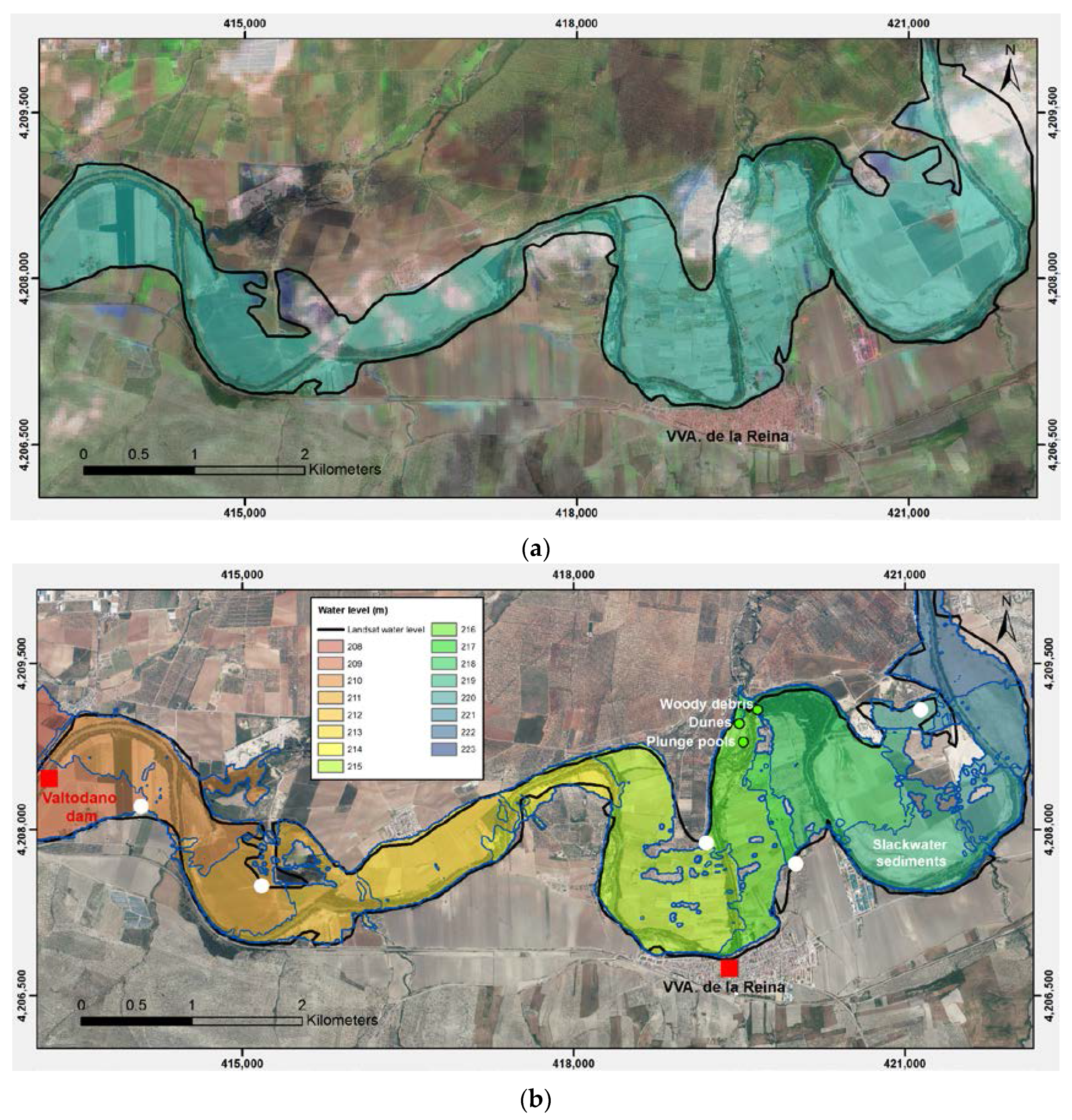
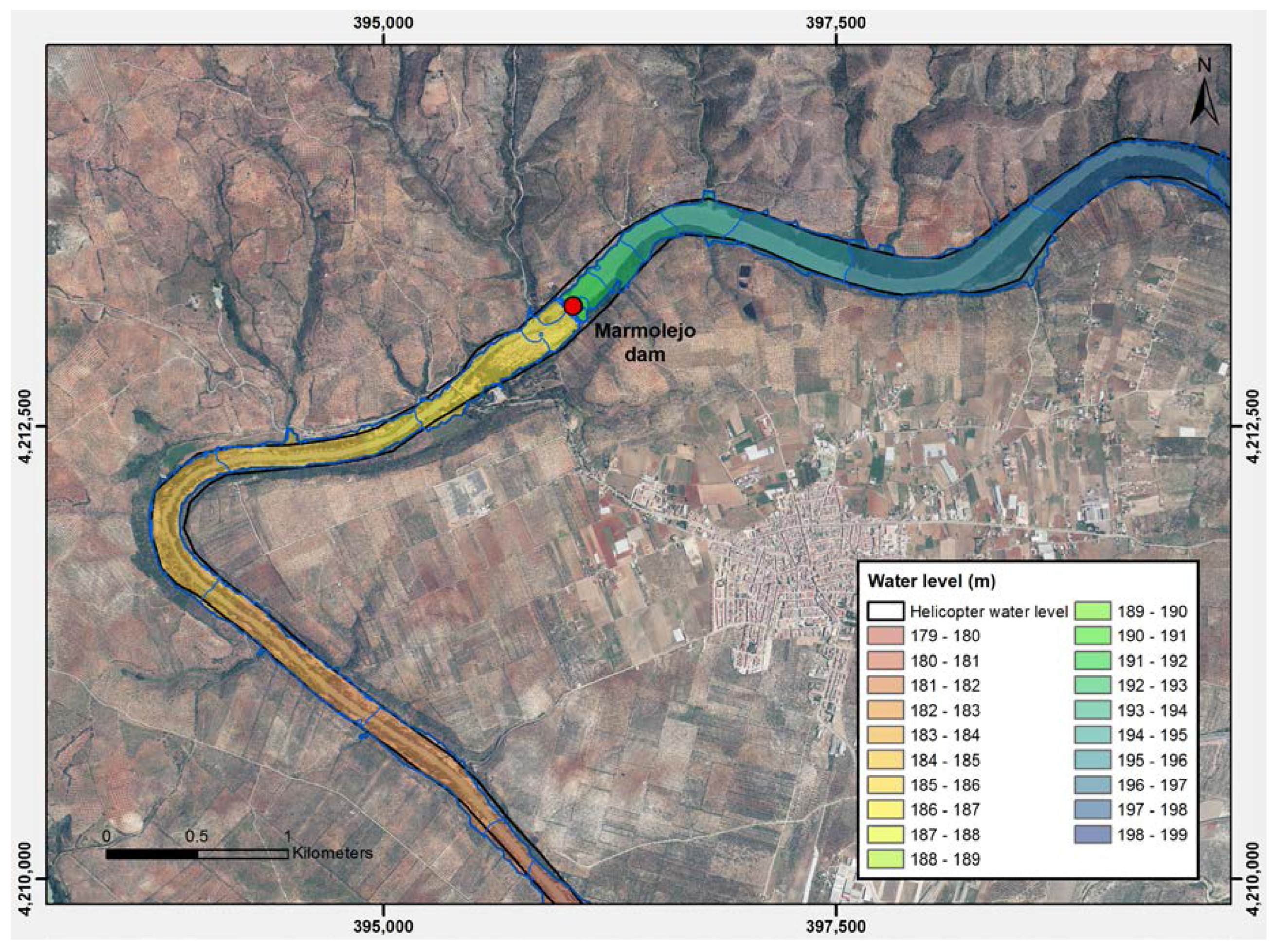
Widespread flood-level rise occurred all over the studied area after impoundment, which reflects a change in channel capacity (denoted from now on by ∆Q_FS). In the confined valley setting, we inferred the accumulated change in channel capacity from the rating curve at flood stage. In the inlet valley (Figure 6), the accumulated reduction in channel capacity amounts to ∆Q_FS = 568 m³·s⁻¹ since 1910 and represents the 56% of the original capacity Q_FS = 1010 m³·s⁻¹ for a 8 m flood depth (see Figure 5a). The major alteration process was the development of a shallow island in the middle of the channel. 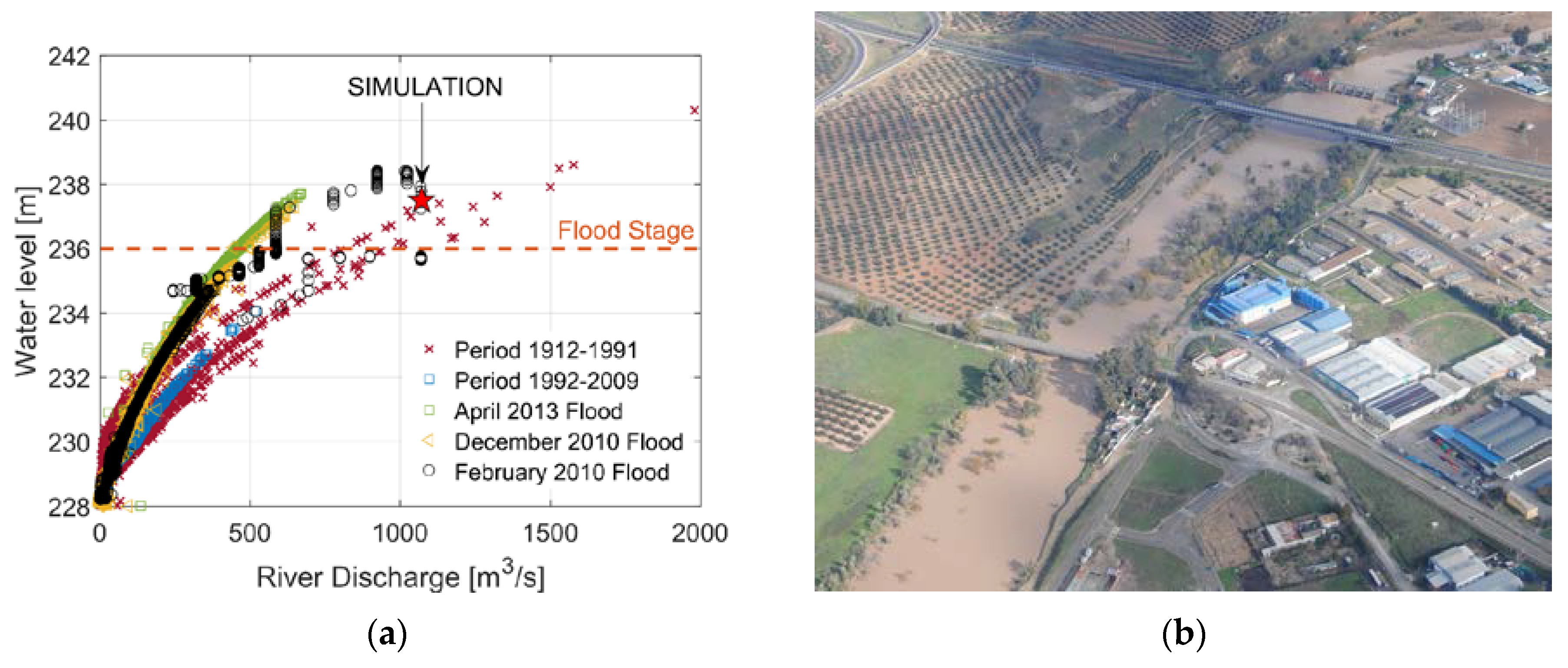It was colonized by non-flexible riparian vegetation (recall Figure 5b) that reduces the mean flow velocity V_FS. In the outlet valley (Figure 7), downstream of the dam, the influence of bank vegetation on channel capacity was moderate (Figure 8a). 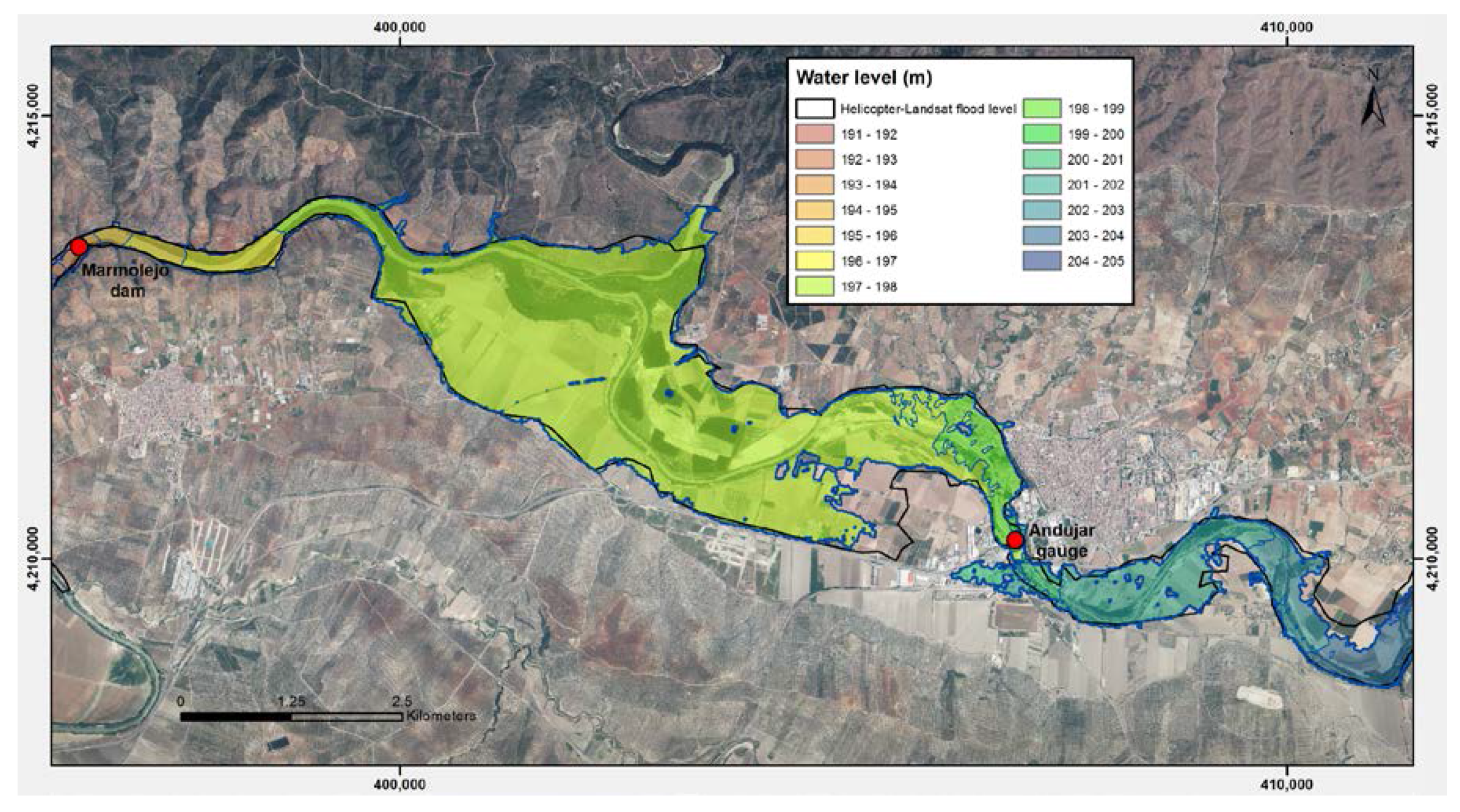Setting a flood depth of 7.2 m yields ∆Q_FS = 188 m³·s⁻¹ for Q_FS = 1565 m³·s⁻¹. In the floodplain downstream of Andújar city (Figure 9), the base-level rise upstream of the silted-up reservoir exacerbated flooding in the period 2009–2013 with respect to the middle of the twentieth century, but the lack of documentary records during the Spanish civil war and the dictatorial regime prevented their analysis.

Alternatively, we followed the original approach by Fergus [47] and characterised ∆Q_FS in terms of the change in cross-sectional channel area at flood stage ∆A_FS.

Table 5. Mean width, depth and channel capacity at flood stage in 1900 and 2013.

River Stretch	1900			2013
	BFS (m)	HFS (m)	AFS (m2)	BFS (m)	HFS (m)	AFS (m2)
City-confluence	121	6.2	711	111	4.3	506
Confluence-valley	138	9.0	1249	100	4.2	448

summarises channel change statistics in twenty cross profiles uniformly distributed from the city to the entrance of the outlet valley with a distance of 400 m between each profile. In the river stretch between the city and the confluence, the channel width (flow depth) at flood stage decreased from 121 (6.2) to 111 (4.3) m during the study period. Downstream of the confluence, the decrease from 138 (9) to 100 and (4.2) m was more pronounced than upstream. Hence, the mean cross-sectional channel area at flood stage A_FS in 1900 was 1249 and 448 m² in the river stretch upstream and downstream of the Guadalquivir-Jándula river confluence. This makes a difference with respect to present days as the actual channel area in each river reach is 448 and 506 m², which amounts to the relative reduction in cross-sectional channel area ∆A_FS/A_FS = 64% and 28%.

In the meandering floodplain (Figure 4), we proceeded to analyse the channel form, a procedure that provides a context for interpretation of past changes in the fluvial environment (Appendix B). We adopted the following two methods to quantify the original channel capacity in the early twentieth century. First, Dury’s algebraic equation was selected from available equations in the paleohydrology literature to estimate pre-impoundment channel capacity using geometrical data of the meanders into the lowest sand-mud terrace [50]. Second, results from regime based equations by Yalin and da Silva [51] linking the bankfull dimensions of the channel and the water discharge served not only to estimate channel capacity pre-impoundment but also to account for changes in channel roughness due to post-impoundment vegetation encroachment.

Substituting the mean wavelength value given in Appendix A into Dury’s correlation (A1), one obtains the pre-impoundment channel capacity Q_FS = 2023 m³·s⁻¹ in the meandering setting. Streamflows larger than 2000 m³·s⁻¹ were required to overtop the river banks and inundate the current floodplain in years previous to flow regulation. A similar result was obtained using equations by Yalin and da Silva [51], who reviewed all the available regime-data before the year 1990 and correlated the bankfull dimensions of the collected rivers and the river discharge. The main advantage of the second approach is that it incorporates the dependency on the roughness coefficient explicitly. In the situation of pre-vegetation encroachment, n = 0.035 s·m^−1/3 [1]. Evaluating (A3) with the mean thalweg slope S₀ = 0.076%, the mean bankfull width B = 184 m and flow depth in the range of 4–5 m, yields 1460 ≤ Q_FS ≤2118 m³·s⁻¹. Note that the upper bound is in close agreement with Dury’s solution Q_FS = 2023 m³·s⁻¹ and the National Database of Historical Floods [29,30], which reported flood episodes only in the years 1963 and 1945 with river discharges in the range of 2500–3000 m³·s⁻¹.

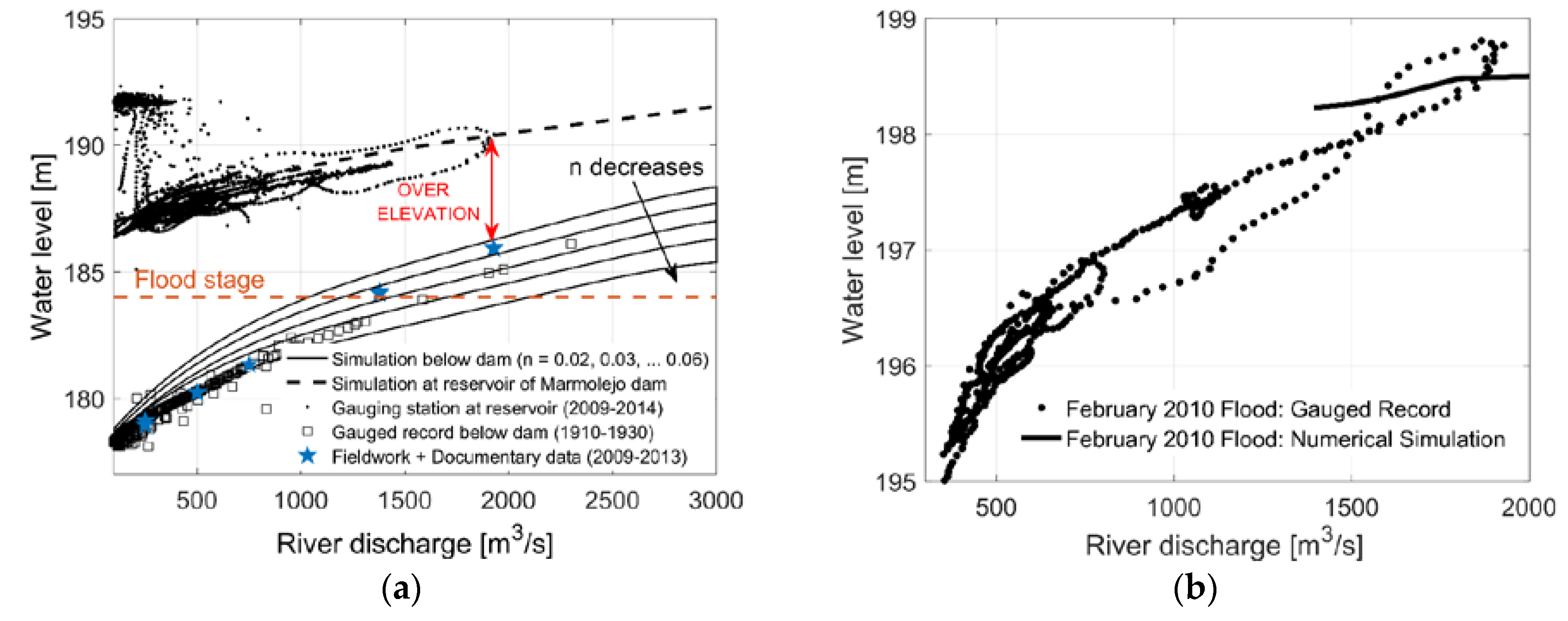
In the current situation of channel infilling and vegetation encroachment, the mean Manning’s roughness increases up to 0.06 s·m^−1/3 (Figure 8a). Such an increase in roughness leads to an overall reduction in channel capacity from 1460 to 852 m³·s⁻¹ for the bankfull flow depth of 4 m. As a matter of fact, inundations of the meandering stretch occurred during the years 2009–2013 at the water discharges of 800–1070 m³·s⁻¹, which is consistent with the prediction of the hydraulic model.

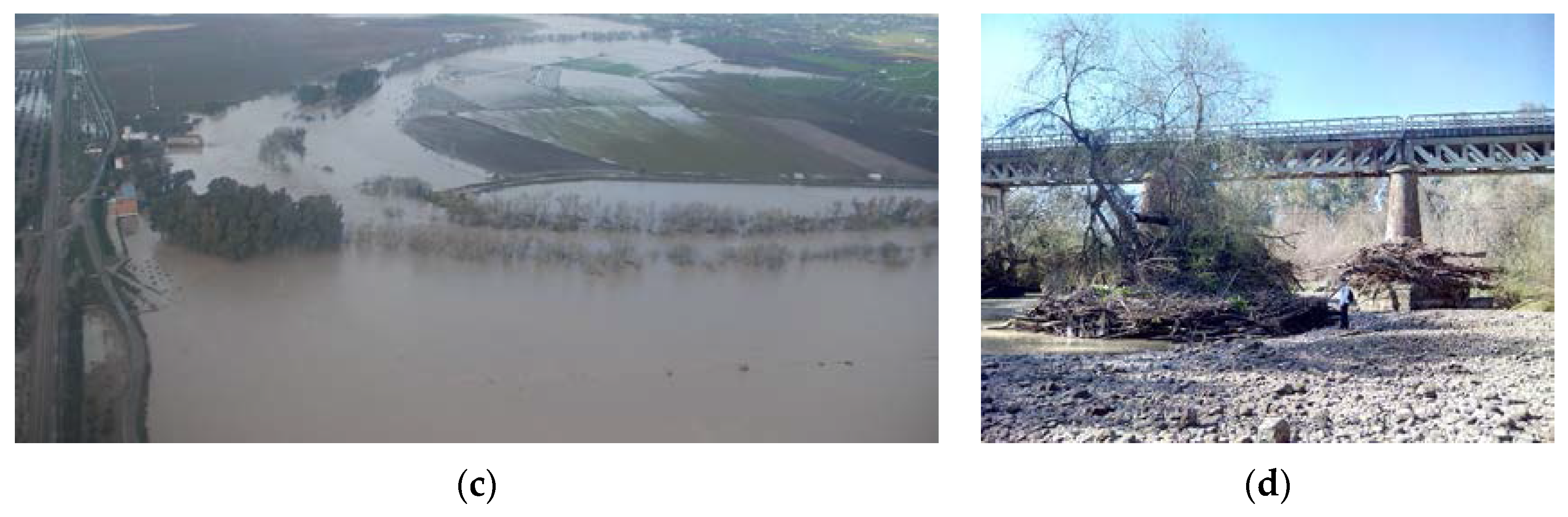
The unexpected increase in inundated areas in the Upper River Basin during extreme rainfall events in 2010–2013 (Figure 4, Figure 6, Figure 7 and Figure 9) contrasts with historical records of inundations before river flow regulation and trends in both precipitation and streamflow during the twentieth century (recall Figure 10). In the inlet valley of the study site, we found flows as deep as 12.3 m with a local streamflow of, approximately, 2000 m³·s⁻¹ in the inundation of the year 1963 (Figure 5a). The rest of floods in the period 1912–2009 were less severe and exhibited flow depths lower than 10.6 m with local river discharges smaller than 1577 m³·s⁻¹ at the same location. Surprisingly, maximum stages in the period 2010–2013 varied in the range of 9.7–10.4 m for streamflows in the range of 670–1024 m³·s⁻¹. Such flow depths are similar in magnitude than in 1924 when the river discharge achieved 1577 m³·s⁻¹. 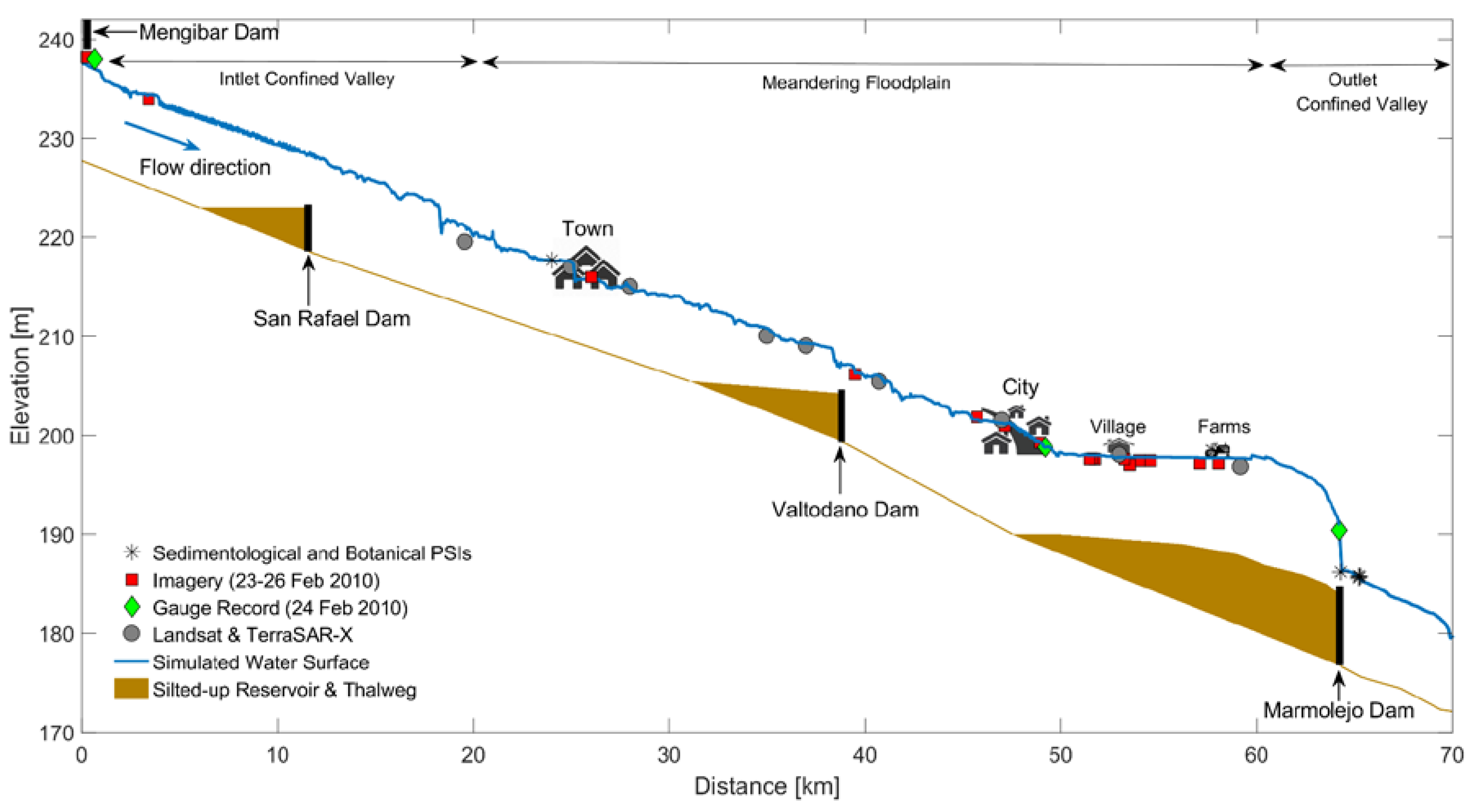Furthermore, flow depths corresponding with a 670 m³·s⁻¹ river discharge increased from 6.7–7.5 m to 9.7 m over the studied period. In the outlet valley, the deepest historical flood developed a flow depth of 8 m for 2300 m³·s⁻¹ that nearly equals the stage of a modern flood with the lower discharge of 1950 m³·s⁻¹. Nonetheless, the observed increase in flood risk during modern floods is due to the decrease in channel capacity post-impoundment.

4.3. Identification of Flood Driver at the Basin Scale

Land degradation processes in the catchment increased sediment yield and availability of fine sediments (mostly, silt and clay). We processed and quantified soil losses across the drainage basin using maps of soil use and vegetation cover between the years 1956, 1984 and 2007 [33]. Nearly half of the area dedicated to olive groves in 2007 currently replaces old arable crops from 1956 (

Table 6. Evolution of soil use in the Guadalquivir basin draining the study area between the years 1956, 1984 and 2007.

	1956		1984		2007
	Area (km2)	Percent	Area (km2)	Percent	Area (km2)	Percent
Arable crops	4990	30	4500	28	2610	16
Olive groves	2585	16	3098	19	4450	28
Scrub/forest	7179	44	7721	48	7838	48
Woody crops	387	3	544	3	591	4
Other	1136	7	295	2	629	4

). Specifically, land-use change since 1956 represents an increase (decrease) in olive groves (arable crops) from 16 (30) to 28 (16) per cent of the drainage area. Theoretical estimates and experimental measurements of mean annual soil loss rates by water erosion for arable crops and olive groves were borrowed from the literature, which yields 3 t·ha⁻¹·year⁻¹ [52] and 60 t·ha⁻¹·year⁻¹ [53], respectively. Scaling these factors by the corresponding areas in Table 6 yields an overall increase of 63% in the mean annual budget of sediments supplied from the basin to the river that raises from 1680 to 2740 t·year⁻¹ between the years 1956 and 2007.

The synergistic effect of increasing sediment supply and decreasing streamflow by flow regulation and climate provoked a widespread aggradation (base-level rise) and reduced channel capacity over time. In the second half of the twentieth century, extraordinary events of high flood recurrence activated sediment transport and geomorphic processes. Dam heightening and exceptional floods in the sixties induced reservoir sedimentation. Streamflow regulation and droughts in the period 1985–1997 favoured in-channel sediment storage. Furthermore, colonisation of sediment deposit by riparian vegetation led to abandonment channel and channel infilling. The channel width decreased at flood stage. This situation prevails along the whole Guadalquivir River nowadays and explains the increase in flood hazard observed in the flood episodes during the period 2009–2013.

5. Conclusions

This article presents the first flood study in the Guadalquivir River (Southern Spain) verifying the outputs of the model simulated inundation extent with respect to remote sensing data. Flood hazard maps computed with the two-dimensional hydraulic model DassFlow-Hydro 2.0 predict reasonably well the observed inundation area derived based on Lansat 5 data at the peak streamflow of approximately 1900 m³·s⁻¹ on 24 February 2010. We improved flood observation for cloud-covered areas and narrow, confined valleys via helicopter flood photographs and field survey of paleostage indicators. The overall accuracy of the modelled flooding area achieves more than 80%, which is a significant achievement regarding previous flood simulation studies with an overlap between modelled and observed extents lower than 70%. The local root mean square error of the simulated and observed water levels varies in the range of 1–8% and 1–5% of the maximum flow depth in the unconfined meandering floodplain and the confined valley setting, respectively.

Based on the above analysis of recent floods, series of orthophotos, historical topographic maps and available rating curves, we analysed the spatiotemporal changes of the Guadalquivir channel capacity over the period 1900–2013. Channel aggradation, reservoir sedimentation and vegetation encroachment are the main factors reducing the channel capacity after river impoundment. In the confined valley, the maximum reduction in channel capacity amounts to ∆Q_FS = 568 m³·s⁻¹ which represents the 56% of the original capacity Q_FS ≈ 1000 m³·s⁻¹ for a 8 m flood depth. In the unconfined floodplain, the decrease in the cross-sectional area upstream of a silted-up reservoir leads to a 28–64% reduction in channel capacity for the undisturbed value 1500 ≤ Q_FS ≤ 2000 m³·s⁻¹.

We conclude that geomorphic processes and anthropogenic alterations of the topography have both mediated and increased the flood risk and backwater effects over time. The observed decrease in channel capacity at flood stage contrasts with the observed and projected decrease of 20–33% in mean annual precipitation and streamflow in the Guadalquivir River under the current scenario of climate change. Hence, the long-term projection of flood risk from existing studies in the Guadalquivir Basin needs to be revisited and account for the probability of a further reduction in channel capacity in addition to the probability of extreme hydrological events and streamflow.

As the Guadalquivir River also flooded across the lower basin and inundated large industrial areas, the analysis in detail of the dynamics of the flood wave deserves an additional study there. To this end, the capabilities of DassFlow-Hydro 2.0 [22] to assimilate remote sensing data via the resolution of the adjoint-based inverse problem could be used instead of the direct flood mapping method adopted in this paper. Furthermore, new studies can be carried out in the Iberian Peninsula on regulated rivers with a similar geomorphic status as the Guadalquivir River (e.g., the Ebro River).

References

1. Bohorquez, P. Paleohydraulic reconstruction of modern large floods at subcritical speed in a confined valley: Proof of concept. Water 2016, 8, 567. [Google Scholar] [CrossRef]
2. Bohorquez, P.; Aranda, V.; Calero, J.; García-García, F.; Ruiz-Ortiz, P.A.; Fernández, T.; Salazar, C. Floods in the Guadalquivir River (Southern Spain). In Proceedings of the International Conference on Fluvial Hydraulics, RIVER FLOW 2014, Lausanne, Switzerland, 3–5 September 2014; pp. 1711–1719. [Google Scholar]
3. European Environment Agency. Climate Change, Impacts and Vulnerability in Europe 2016: An Indicator-Based Report; Publications Office of the European Union: Luxembourg, 2017; Available online: https://www.eea.europa.eu/publications/climate-change-impacts-and-vulnerability-2016 (accessed on 26 January 2017).
4. Intergovernmental Panel on Climate Change (IPCC). Climate Change 2013: The Physical Science Basis. Contribution of Working Group I to the Fifth Assessment Report of the Intergovernmental Panel on Climate Change; Stocker, T.F., Qin, D., Plattner, G.-K., Tignor, M.M.B., Allen, S.K., Boschung, J., Nauels, A., Xia, Y., Bex, V., Midgley, P.M., Eds.; Cambridge University Press: Cambridge, UK; New York, NY, USA, 2013. [Google Scholar]
5. Slater, L.J.; Singer, M.B.; Kirchner, J.W. Hydrologic versus geomorphic drivers of trends in flood hazard. Geophys. Res. Lett. 2015, 42, 370–376. [Google Scholar] [CrossRef]
6. Walter, R.C.; Merritts, D.J. Natural streams and the legacy of water-powered mills. Science 2008, 319, 299–304. [Google Scholar] [CrossRef] [PubMed]
7. Naylor, L.A.; Spencer, T.; Lane, S.N.; Darby, S.E.; Magilligan, F.J.; Macklin, M.G.; Möller, I. Stormy geomorphology: Geomorphic contributions in an age of climate extremes. Earth Surf. Process. Landf. 2017, 42, 166–190. [Google Scholar] [CrossRef]
8. Nied, M.; Schröter, K.; Lüdtke, S.; Nguyen, V.D.; Merz, B. What are the hydro-meteorological controls on flood characteristics? J. Hydrol. 2017, 545, 310–326. [Google Scholar] [CrossRef]
9. De Moel, H.; van Alphen, J.; Aerts, J.C.J.H. Flood maps in Europe—Methods, availability and use. Nat. Hazards Earth Syst. Sci. 2009, 9, 289–301. [Google Scholar] [CrossRef]
10. Alfieri, L.; Salamon, P.; Bianchi, A.; Neal, J.; Bates, P.; Feyen, L. Advances in pan-European flood hazard mapping. Hydrol. Process. 2014, 28, 4067–4077. [Google Scholar] [CrossRef]
11. Nones, M.; Gerstgraser, C.; Wharton, G. Consideration of hydromorphology and sediment in the implementation of the EU water framework and floods directives: A comparative analysis of selected EU member states. Water Environ. J. 2017. [Google Scholar] [CrossRef]
12. Costabile, P.; Macchione, F. Enhancing river model set-up for 2-D dynamic flood modelling. Environ. Model. Softw. 2015, 67, 89–107. [Google Scholar] [CrossRef]
13. Lorenzo-Lacruz, J.; Vicente-Serrano, S.M.; López-Moreno, J.I.; Morán-Tejeda, E.; Zabalza, J. Recent trends in Iberian streamflows (1945–2005). J. Hydrol. 2012, 414–415, 463–475. [Google Scholar] [CrossRef]
14. Alfieri, L.; Burek, P.; Feyen, L.; Forzieri, G. Global warming increases the frequency of river floods in Europe. Hydrol. Earth Syst. Sci. 2015, 19, 2247–2260. [Google Scholar] [CrossRef]
15. Toonen, W.H.J.; Middelkoop, H.; Konijnendijk, T.Y.M.; Macklin, M.G.; Cohen, K.M. The influence of hydroclimatic variability on flood frequency in the Lower Rhine. Earth Surf. Process. Landf. 2016, 41, 1266–1275. [Google Scholar] [CrossRef]
16. Baker, V.R. Paleoflood hydrology: Origin, progress, prospects. Geomorphology 2008, 101, 1–13. [Google Scholar] [CrossRef]
17. Benito, G.; Lang, M.; Barriendos, M.; Llasat, M.C.; Francés, F.; Ouarda, T.; Thorndycraft, V.; Enzel, Y.; Bardossy, A.; Coeur, D.; et al. Use of systematic, palaeoflood and historical data for the improvement of flood risk estimation. Review of scientific methods. Nat. Hazards 2004, 31, 623–643. [Google Scholar] [CrossRef]
18. Olthof, I. Mapping seasonal inundation frequency (1985–2016) along the St-John River, New Brunswick, Canada using the Landsat archive. Remote Sens. 2017, 9, 143. [Google Scholar] [CrossRef]
19. Schumann, G.J.-P.; Neal, J.C.; Mason, D.C.; Bates, P.D. The accuracy of sequential aerial photography and SAR data for observing urban flood dynamics, a case study of the UK summer 2007 floods. Remote Sens. Environ. 2011, 115, 2536–2546. [Google Scholar] [CrossRef]
20. Seier, G.; Stangl, J.; Schöttl, S.; Sulzer, W.; Sass, O. UAV and TLS for monitoring a creek in an alpine environment, Styria, Austria. Int. J. Remote Sens. 2017, 38, 2903–2920. [Google Scholar] [CrossRef]
21. Bohorquez, P.; García-García, F.; Pérez-Valera, F.; Martínez-Sánchez, C. Unsteady two-dimensional paleohydraulic reconstruction of extreme floods over the last 4000 year in Segura River, southeast Spain. J. Hydrol. 2013, 477, 229–239. [Google Scholar] [CrossRef]
22. Monnier, J.; Couderc, F.; Dartus, D.; Larnier, K.; Madec, R.; Vila, J.-P. Inverse algorithms for 2D shallow water equations in presence of wet dry fronts: Application to flood plain dynamics. Adv. Water Resour. 2016, 97, 11–24. [Google Scholar] [CrossRef]
23. Bohorquez, P.; Darby, S.E. The use of one- and two-dimensional hydraulic modelling to reconstruct a glacial outburst flood in a steep Alpine valley. J. Hydrol. 2008, 361, 240–261. [Google Scholar] [CrossRef]
24. Hall, J.; Arheimer, B.; Borga, M.; Brázdil, R.; Claps, P.; Kiss, A.; Kjeldsen, T.R.; Kriaučiūnienė, J.; Kundzewicz, Z.W.; Lang, M.; et al. Understanding flood regime changes in Europe: A state-of-the-art assessment. Hydrol. Earth Syst. Sci. 2014, 18, 2735–2772. [Google Scholar] [CrossRef]
25. Barredo, J.I.; Saurí, D.; Llasat, M.C. Assessing trends in insured losses from floods in Spain 1971–2008. Nat. Hazards Earth Syst. Sci. 2012, 12, 1723–1729. [Google Scholar] [CrossRef]
26. Seminara, G. Meanders. J. Fluid Mech. 2006, 554, 271–297. [Google Scholar] [CrossRef]
27. MAGRAMA (Ministerio de Agricultura y Pesca, Alimentación y Medio Ambiente). Sistema de Información del Anuario de Aforo. Available online: http://sig.magrama.es/aforos (accessed on 1 September 2015).
28. CHG (Confederación Hidrográfica del Guadalquivir). Sistema Automático de Información Hidrológica de la Cuenca del Guadalquir. Available online: http://www.chguadalquivir.es/saih/ (accessed on 1 September 2015).
29. Pascual, G.; Bustamante, A. Catálogo Nacional de Inundaciones Históricas. Actualización; Ministerio del Interior: Madrid, Spain, 2011. [Google Scholar]
30. Disaster Information Management System. Available online: http://www.desinventar.net (accessed on 1 September 2015).
31. Institute of Statistics and Cartography of Andalusia. Digital Catalogue of Historical Cartography. Available online: http://www.juntadeandalucia.es/institutodeestadisticaycartografia/cartoteca (accessed on 1 September 2015).
32. Spanish National Geographic Institute (IGN). Topographic Archive. Available online: http://www.ign.es/web/mapasantiguos (accessed on 1 September 2015).
33. Environmental Information Network of Andalusia (REDIAM). Comparador WMS Ortofotos; Cartografía de Inundaciones en Febrero-Marzo 2010 en las Cuencas de los ríos Guadalquivir y Guadalete; Mapa de usos y Coberturas Vegetales Multitemporal. Available online: http://www.juntadeandalucia.es/medioambiente/site/rediam (accessed on 1 September 2015).
34. Roy, D.P.; Ju, J.; Kline, K.; Scaramuzza, P.L.; Kovalskyy, V.; Hansen, M.; Loveland, T.R.; Vermote, E.; Zhang, C. Web-enabled Landsat Data (WELD): Landsat ETM+ composited mosaics of the conterminous United States. Remote Sens. Environ. 2010, 114, 35–49. [Google Scholar] [CrossRef]
35. Spanish National Geographic Institute (IGN). Plan Nacional de Ortofotografía Aérea. Available online: http://pnoa.ign.es/ (accessed on 1 September 2015).
36. Blocken, B.; Gualtieri, C. Ten iterative steps for model development and evaluation applied to Computational Fluid Dynamics for Environmental Fluid Mechanics. Environ. Model. Softw. 2012, 33, 1–22. [Google Scholar] [CrossRef]
37. Arcement, G.J., Jr.; Schneider, V.R. Guide for Selecting Manning’s Roughness Coefficients for Natural Channels and Flood Plains; United States Government Printing Office: Denver, CO, USA, 1989; Volume 2339.
38. Carling, P.A.; Herget, J.; Lanz, J.K.; Richardson, K.; Pacifici, A. Channel-scale erosional bedforms in bedrock and in loose granular material: Character, processes and implications. In Megaflooding on Earth and Mars; Burr, D.M., Carling, P.A., Baker, V.R., Eds.; Cambridge University Press: Cambridge, UK, 2009; pp. 13–32. [Google Scholar]
39. Baker, V.R. The channeled scabland: A retrospective. Annu. Rev. Earth Planet. Sci. 2009, 37, 393–411. [Google Scholar] [CrossRef]
40. Bates, P.; de Roo, A.P. A simple raster-based model for flood inundation simulation. J. Hydrol. 2000, 236, 54–77. [Google Scholar] [CrossRef]
41. Wood, M.; Hostache, R.; Neal, J.; Wagener, T.; Giustarini, L.; Chini, M.; Corato, G.; Matgen, P.; Bates, P. Calibration of channel depth and friction parameters in the LISFLOOD-FP hydraulic model using medium-resolution SAR data and identifiability techniques. Hydrol. Earth Syst. Sci. 2016, 20, 4983–4997. [Google Scholar] [CrossRef]
42. Aronica, G.; Bates, P.D.; Horritt, M.S. Assessing the uncertainty in distributed model predictions using observed binary pattern information within GLUE. Hydrol. Process. 2002, 16, 2001–2016. [Google Scholar] [CrossRef]
43. Veilleux, A.G.; Cohn, T.A.; Flynn, K.M.; Mason, R.R., Jr.; Hummel, P.R. Estimating Magnitude and Frequency of Floods Using the PeakFQ 7.0 Program; Fact Sheet 2013-3108; USGS Publications Warehouse: Reston, VA, USA, 2014.
44. Seiler, R.A.; Hayes, M.; Bressan, L. Using the standardized precipitation index for flood risk monitoring. Int. J. Climatol. 2002, 22, 1365–1376. [Google Scholar] [CrossRef]
45. Agnew, C.T. Using the SPI to identify drought. Drought Netw. News 2010, 12, 6–11. [Google Scholar]
46. Gregory, K.J.; Park, C. Adjustment of river channel capacity downstream from a reservoir. Water Resour. Res. 1974, 10, 870–873. [Google Scholar] [CrossRef]
47. Fergus, T. Geomorphological response of a river regulated for hydropower: River Fortun, Norway. Regul. Rivers Res. Manag. 1997, 13, 449–461. [Google Scholar] [CrossRef]
48. Masterman, R.; Thorne, C.R. Predicting influence of bank vegetation on channel capacity. J. Hydraul. Eng. 1992, 118, 1052–1058. [Google Scholar] [CrossRef]
49. Jacobson, R.B.; O’Connor, J.E.; Oguchi, T. Surficial geological tools in fluvial geomorphology. In Tools in Fluvial Geomorphology; Kondolf, G.M., Piégay, H., Eds.; John Wiley & Sons, Ltd.: Chichester, UK, 2016; pp. 11–39. ISBN 978-111-864-855-1. [Google Scholar]
50. Williams, G.P. Paleohydrologic Equations for Rivers. In Developments and Applications of Geomorphology; Costa, J.E., Fleisher, P.J., Eds.; Springer: Berlin/Heidelberg, Germany, 1984; pp. 343–367. ISBN 978-364-269-759-3. [Google Scholar]
51. Yalin, M.S.; da Silva, A.M.F. Fluvial Processes; IAHR Monograph; IAHR: Delft, The Netherlands, 2001. [Google Scholar]
52. Panagos, P.; Borrelli, P.; Poesen, J.; Ballabio, C.; Lugato, E.; Meusburger, K.; Montanarella, L.; Alewell, C. The new assessment of soil loss by water erosion in Europe. Environ. Sci. Policy 2015, 54, 438–447. [Google Scholar] [CrossRef]
53. Vanwalleghem, T.; Amate, J.I.; de Molina, M.G.; Fernández, D.S.; Gómez, J.A. Quantifying the effect of historical soil management on soil erosion rates in Mediterranean olive orchards. Agric. Ecosyst. Environ. 2011, 142, 341–351. [Google Scholar] [CrossRef]
54. Dury, G.H. Discharge prediction, present and former, from channel dimensions. J. Hydrol. 1976, 30, 219–245. [Google Scholar] [CrossRef]
Figure 1. Study area along the Guadalquivir River including the inundated area (light blue) on 24 February 2010 for Q = 1950 m3·s−1 at Marmolejo dam (flow from right to left). Urban areas at risk and hydropower stations are highlighted in red and yellow, respectively. Aerial photography shows a small portion of flooded areas in Llanos del Sotillo. Our earlier work [1] presents a detailed analysis of the flood dynamics in the confined valley of 6 km length downstream of Marmolejo dam.
Remotesensing 09 00727 g001
Figure 2. Hydrograph showing river discharges at: Zocueca (1); Encinarejo (2); Mengíbar (3); and Marmolejo (4) dams in February 2010.
Remotesensing 09 00727 g002
Figure 3. Longitudinal profile of maximum water levels in the numerical flood simulation (solid blue line) on 24 February 2010 with 2000 m3·s−1 streamflow in Marmolejo dam. Flow from left to right.
Remotesensing 09 00727 g003
Figure 4. (a) Flooded area derived based on Lansat 5 data and corrected with flood photographs on 24 February 2010; (b) Numerical flood simulation superposed on Lansat wet perimeter. Colours indicate altitudes of water surface. Flow from right to left. The inundated town at the bottom is Villanueva de Reina. Stage indicators correspond with Figure 3; (c) Photograph of the overtopped Valtodano dam (see location in panel b); (d) An example of botanical HWM-PSI. Person 1.85 m tall provides scale.
Remotesensing 09 00727 g004aRemotesensing 09 00727 g004b
Figure 5. (a) Rating curves at stream gauges (650 m downstream of Mengíbar dam); and (b) flooded area downstream of Mengíbar dam on 8 December 2010 with the local river discharge Q = 650 m3·s−1 (flow from top to bottom). Gauge stations located on the second bridge.
Remotesensing 09 00727 g005
Figure 6. (a) Simulated and observed inundation extent, together with slackwater deposits; (b) map of simulated velocity magnitude; and (c) contours of modelled water surface elevation.
Remotesensing 09 00727 g006
Figure 7. Contours of water elevation from the numerical flood simulation (transparent colour) and inundation perimeter derived based on helicopter flood photograph (black line) on 24 February 2010 at the outlet confined valley crossing Marmolejo dam (red dot). Flow from right to the bottom.
Remotesensing 09 00727 g007
Figure 8. Measured and simulated rating curves at stream gauges: (a) reservoir and foot of Marmolejo dam; and (b) Roman Bridge of Andújar city. Panel (a) includes a sensitivity study of the model results downstream of Marmolejo dam with variations in the Manning’s roughness coefficient.
Remotesensing 09 00727 g008
Figure 9. Numerical flood simulation (coloured transparent contour) and flooded area derived based on Landsat/TerraSAR-X/helicopter data (solid line in black) on 24 February 2010. The location of Marmolejo dam and the stream gauge near Andújar city is also given. Flow from right to left.
Remotesensing 09 00727 g009
Figure 10. (a) Flood frequency distribution and relative magnitude of the Guadalquivir River floods at Marmolejo dam (after [1]); and (b) flood frequency analysis of streamflow records using PeakFQ [43]. Estimates of flood magnitudes for several recurrence intervals (1–200 years) are also given.
Remotesensing 09 00727 g010