Article

An Accuracy Assessment of Derived Digital Elevation Models from Terrestrial Laser Scanning in a Sub-Tropical Forested Environment

1
Joint Remote Sensing Research Program, School of Earth and Environmental Sciences, University of Queensland, St. Lucia, Brisbane 4067, Queensland, Australia
2
Department of Science, Information Technology and Innovation (DSITI) Remote Sensing Centre, Ecosciences Precinct, Brisbane 4001, Queensland, Australia
3
School of Science and Technology, University of New England, Armidale 2350, New South Wales, Australia
4
Department of Geographical Sciences, University of Maryland, College Park, MD 20742, USA
*
Author to whom correspondence should be addressed.
Submission received: 15 June 2017 / Revised: 28 July 2017 / Accepted: 9 August 2017 / Published: 14 August 2017
(This article belongs to the Section Forest Remote Sensing)

Abstract

:
Forest structure attributes produced from terrestrial laser scanning (TLS) rely on normalisation of the point cloud values from sensor coordinates to height above ground. One method to do this is through the derivation of an accurate and repeatable digital elevation model (DEM) from the TLS point cloud that is used to adjust the height. The primary aim of this paper was to test a number of TLS scan configurations, filtering options and output DEM grid resolutions (from 0.02 m to 1.0 m) to define a best practice method for DEM generation in sub-tropical forest environments. The generated DEMs were compared to both total station (TS) spot heights and a 1-m DEM generated from airborne laser scanning (ALS) to assess accuracy. The comparison to TS spot heights found that a DEM produced using the minimum elevation (minimum Z value) from a point cloud derived from a single scan had mean errors >1 m for DEM grid resolutions <0.2 m at a 25-m plot radius. At a 1-m grid resolution, the mean error was 0.19 m. The addition of a filtering approach that combined a median filter with a progressive morphological filter and a global percentile filter was able to reduce mean error of the 0.02-m grid resolution DEM to 0.31 m at a 25-m plot radius using all returns. Using multiple scan positions to derive the DEM reduced the mean error for all DEM methods. Our results suggest that a simple minimum Z filtering DEM method using a single scan at the grid resolution of 1 m can produce mean errors <0.2 m, but for a small grid resolution, such as 0.02 m, a more complex filtering approach and multiple scan positions are required to reduced mean errors. The additional validation data provided by the 1-m ALS DEM showed that when using the combined filtering method on a point cloud derived from a single scan at the plot centre, errors between 0.1 and 0.5 m occurred in the TLS DEM for all tested grid resolutions at a plot radius of 25 m. These findings present a protocol for DEM production from TLS data at a range of grid resolutions and provide an overview of factors affecting DEMs produced from single and multiple TLS scan positions.

Graphical Abstract

1. Introduction

Extraction of forest structure attributes, such as stem density, diameter at breast height (DBH), basal area (BA), tree height, biomass, plant area index (PAI) and canopy density from LiDAR (light detection and ranging), has become an important method to inventory and monitor forest resources, and for informing forest management and conservation policy development [1,2,3,4,5]. Terrestrial LiDAR, also known as terrestrial laser scanning (TLS), can be used to measure and estimate these forest structure attributes at single-tree and plot levels [3,6,7]. Although structure attributes derived from TLS data are generally limited in extent to plot-level estimates due to scanning logistics (i.e., field operation time), these attributes can be used as predictors in regression models or machine learning algorithms to estimate structure from datasets over regional to global areas, i.e., airborne laser scanning (ALS) and multispectral or synthetic aperture radar (SAR) satellite imagery [8]).
Multi-temporal TLS measurements can be used to assess change over time in forest structure attributes [9,10,11,12]. However, the measurement of forest structure attributes must be able to detect “true” change, not “false” change detected from incorrect sensor settings, scanner placement or data post-processing. Accurately measuring forest structure attributes, such as understorey height and cover, first requires normalisation of TLS point heights to height above ground. For single-tree measurement, it is possible to normalise the point cloud height by placement of a marker at a pre-defined height. However, for cases where whole of plot forest attributes are to be derived and the site terrain is complex, the placement of a very large number of markers would be required, making this method too time intensive to be practical.
Creating an accurate DEM for normalising of the point cloud to height above ground ensures that TLS structure measurements collected at the plot level are accurate, repeatable and able to be used to detect and measure change. The accuracy of the DEM used to adjust point height, to a height above ground, is a significant control on differences in the estimation of forest structure attributes commonly reported in the literature [13]. In flat, open sites, the ground will not be obscured. However, forested and sloped environments are more complex than “open” landscapes. Trees occlude the ground behind them, and it is necessary to obtain multiple scans to remove or reduce occlusion.
Both ALS and TLS have been used routinely to characterize the ground surface [14,15,16,17]. ALS is able to characterize the ground over large areas, with the point density usually within 2–20 points per square metre. ALS providers generally undertake a vertical accuracy assessment, with a typical user specification being ±20 cm at a 95% confidence interval of survey control. TLS captures a more detailed representation of the ground surface than is possible with ALS, by generating highly accurate points (millimetre accuracy) with typically hundreds of ground points per square metre (depending on distance from the scanner and instrument settings). DEMs have been developed from TLS and their accuracy assessed in the surveying and geomorphology applications [15,18]. In forested environments, although the majority of published studies estimating forest structure attributes use DEMs derived from TLS point clouds, the accuracy of DEMs derived from TLS and the DEM influence on the accuracy of estimated forest structure attributes has not been widely investigated.
The primary aim of this paper was to test a number of TLS scan configurations, filtering options and output DEM pixel sizes, to define a best practise method for DEM generation in sub-tropical forest environments. This was achieved by addressing four objectives:
  • To assess TLS DEM accuracy by comparing DEMs generated from TLS to total station (TS) spot heights.
  • To compare a 1-m resolution DEM generated from ALS to TS spot heights, to determine if ALS can be used for accuracy assessment of a TLS DEM and if an ALS DEM can be used as a replacement for a TLS DEM for normalisation of the TLS point cloud height.
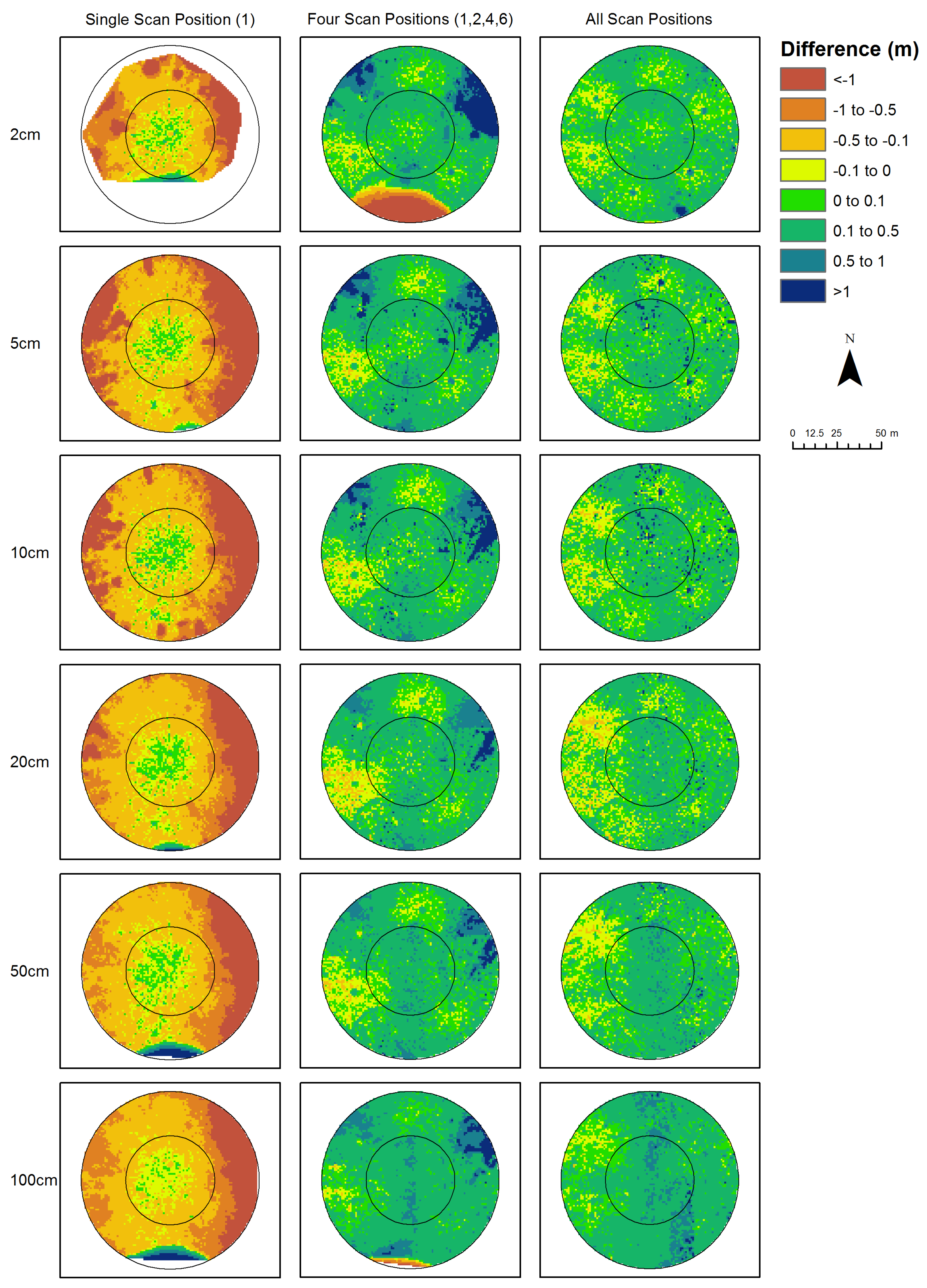
  • To compare DEMs generated from TLS to a 1-m resolution DEM generated from ALS to determine the spatial pattern of errors occurring in the TLS DEM.
  • To assess the repeatability of TLS DEM generation in sub-tropical forests, by evaluating error statistics for three consecutive TLS campaigns in this environment.
To assess the accuracy of a TLS DEM, it is necessary to obtain a validation dataset of a higher order of accuracy. A TS is capable of providing the ground classification certainty and elevation accuracy necessary to provide a reliable set of data for accuracy assessment (where one is certain the pole and prism used with the TS are on the ground) [15]. However, due to survey time requirements, the position of only a limited number of points can be measured with a TS, so the accuracy of the DEM can only be sampled at these locations [18]. Other research has used ALS to assess the accuracy of TLS-derived DEMs [13]. Using ALS data has the benefit of greater spatial coverage than can realistically be collected with a TS. However, further research is needed to determine ALS dataset accuracy under trees. This can be achieved by comparing the ALS DEM to the TS spot heights, to validate its elevation accuracy at the local study site. This will determine if the ALS DEM is suitable for validation of TLS DEMs or as a replacement for a TLS DEM in normalising the TLS point cloud to height above ground.

1.1. Background

Producing an accurate ground representation from LiDAR has proven to be a difficult problem to solve [19]. A review of the literature on DEMs produced from TLS in forested environments showed a number of different methods, using between 1–24 scans and with grid resolutions ranging from 0.02 m–8 m (Table 1). Studies estimating forest structure attributes from TLS often apply algorithms developed for DEM generation with ALS data, even though there are significant differences in point density and viewing geometry between these two types of LiDAR, which may mean that DEM development methods from ALS are not best suited to TLS datasets [20,21]. For example, due to the overhead and vertical acquisition of ALS, the pulse angle is less affected by foreground objects obscuring the ground surface (except in very dense canopies), as opposed to side-view TLS acquisition, where trees and grass block the laser pulse reaching the ground. In addition, ALS is captured in a broad nadir swath, whereas TLS is acquired in a horizontal radial acquisition pattern around the scanner location.
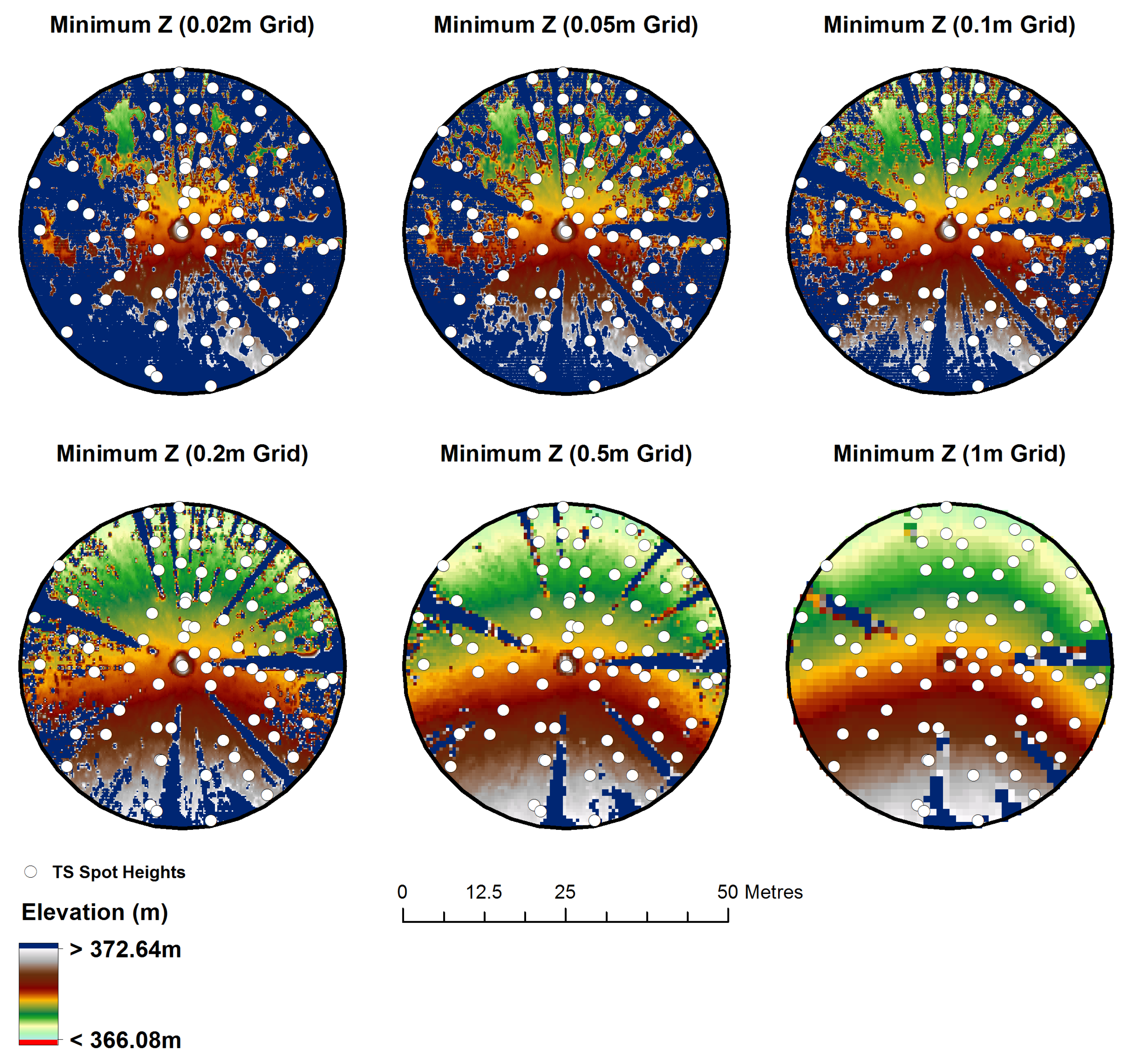
The simplest approach for TLS DEM generation is to use a height adjustment based on scanner height, which may be sufficient where the site is flat [13], but unlikely to be sufficient in sloping sites. Nearly all TLS studies use a minimum elevation (subsequently referred to as the minimum Z value to avoid confusion between scan and projected coordinates) within a specified bin size (i.e., 0.5 × 0.5 m in the X,Y coordinate plane) as the first step to determine ground points [13,15,21,22,23]. Other filters are then typically applied to further filter the dataset to only ground points. These include slope threshold [21], morphological filters [24], median filters [15], or a surface-fitting algorithm through the minimum Z values, i.e., RANSAC [23], linear plane fitting [13], or splines, and then, all points within a specified height threshold from this plane are classified as ground [21,23]. Morphological filters, which rely on an iterative change in window size, as well as slope and height thresholds, are often commonly applied to the generation of DEMs from airborne LiDAR [17,25]; however, only one example was found as applied to TLS [24]. A number of different interpolation methods was found for airborne LiDAR including nearest neighbour, natural neighbour, inverse distance weighting (IDW), kriging and bilinear interpolation [2,26,27], but again, their application to TLS data was a relatively limited subset of that used for ALS datasets.
Three validation data sources were found: ALS [13,21], TS [15] and data derived from the TLS point cloud [24]; while some studies reported no error attributes [22,23]. The methods used by [15,24] have the lowest reported errors, at grid resolutions of less than 1 m.
Based on this review of literature, we chose a method for DEM generation that combines the methods of [11,24] using a morphological filter and median filter, with a natural neighbour interpolation. The morphological filter was chosen for testing due to its successful and widespread use in ALS DEM generation [17,25] and current limited application, but promising results with TLS DEM generation [24]. Chaplot et al. [28] found that where point density was high (as in a TLS scan) the choice of interpolation method made little difference to the errors in the derived DEM; however, where point density was low, the spatial structure of the landscape influenced which interpolator performed the best, suggesting that with TLS, the interpolator is not likely to be a major influence on DEM accuracy. We chose natural neighbour interpolation, as it does not change the value of existing data points and produces interpolated values within the range of the input values. This is unlike some other interpolation methods, such as IDW or splines, that produce interpolated values at the original data point locations that are very close to the original values, but not exactly the same [29].

2. Materials and Methods

2.1. Study Site

The study site used for method development and with TS spot heights was located at an open forest (Eucalyptus spp.) long-term monitoring site known as Landers Hut 3 (code: GOLD0101) in D’Aguilar National Park near Brisbane, Queensland, Australia (~250 km2 in size) (Figure 1). The study site was defined by two plot radii (25 m and 50 m) both of which had their origin at 27 25 44.55 S 152 49 37.44 E. The GOLD0101 site has a mean slope of approximately 8 degrees, with the majority of the slope between 5 and 20 degrees as derived from airborne LiDAR captured in 2014. It has an understorey with long dense grass cover, some shrubs and woody debris and mature trees with heights up to 35 m. It is the same site described in [13].

2.2. Data

2.2.1. TS Data

Two permanent survey marks (PSMs) in conjunction with seven Topcon HiPer SR GNSS receivers were used to establish site control and link to the Queensland Ellipsoidal Height Adjustment (QEHA) and the Australian Height Datum (AHD). Five permanent control points (PCPs) were installed on-site to allow for known and repeatable control between scanning campaigns (Figure 1).
A total of 171 TS spot heights were collected within a 50-m radius of the plot centre and adjusted using Trimble Business Centre to process the static GNSS observations (note: spot heights were also collected outside this area, although not used in this analysis). The location of each TS spot height was chosen so that spot heights were spread across the study plot as shown in Figure 1. Additional points were collected in depressions and over mounds to accurately characterise the elevation features. All points had an overall maximum uncertainty of less than ±0.016 m in the horizontal and vertical directions. The measurement error associated with the PSM on site was less than ±0.021 m and ±0.040 m, respectively in the horizontal and vertical directions. Survey was completed on 23–24 November 2015.

2.2.2. TLS Data

A RIEGL VZ400 commercial terrestrial laser scanner was used to collect the terrestrial LiDAR data. The instrument is a time-of-flight laser scanner, has a laser wavelength of 1550 nm (near infra-red) and can detect multiple discreet returns (up to four recorded automatically). The RIEGL VZ400 has a 30–130-degree field of view when vertically positioned, with a tilt mount necessary to capture the overhead zenith angles. For this study, we have chosen to only use scans acquired in the vertical position, as the vertical scans capture a full 360 degrees in relation to the ground. The scanner was configured not to capture points closer than 0.5 m. The instrument has a beam divergence of 0.35 mrad and was configured to use a pulse repetition frequency of 300 kHz, with pulses emitted at every 0.04- or 0.06-degree increment (depending on the survey date). Relative reflectance is calculated onboard the instrument, as the ratio of the return amplitude to the predicted amplitude for a Lambertian surface at the given range. The return difference from the expected system response is recorded as the deviation, with a higher deviation indicating that the return does not match the expected return and is likely to be from a partial beam interception or a close range second interception [28], and lower deviations are likely to be from a hard surface where the beam is fully intercepted, i.e., ground or trunk.
Seven scan positions were acquired at the GOLD0101 site for each of three dates: 25 November 2015, 27 November 2015 and 9 February 2017. All scans acquired in 2015 used a 0.04-degree pulse increment, while those acquired in 2017 used a 0.06-degree increment. The dataset acquired on 27 November 2015 was used for the main analysis with the other two dates used to assess repeatability. Scans were completed at seven scan positions as shown in Figure 1, with scan positions in the outer circle collected at 33.3 m from the centre scan (Scan Position 1) and 60 degrees apart.
The scans were registered using an automated registration process described in detail in Goodwin et al. [15]. Point clouds from individual scans were aligned using highly reflective targets (10-cm cylinders placed on a pole approximately 1.3 m from the ground) distributed across the study plot. A reflective target was precisely positioned over each of the five PCPs marked during the TS survey campaign, at a known height of 1.8 m using a survey-grade bipod. These five reflective targets were used to tie the scan positions to real-world coordinates in the Map Grid Australia Zone 56 projection (EPSG: 28356). A total of 35 reflective targets were used with locations chosen so that the targets were widely distributed throughout the plot (50-m radius), and at least four targets were visible from each scan position (Figure 2). The root mean squared error (RMSE) for each of the three TLS survey dates was less than 0.02 m for all scan positions (Table 2).

2.2.3. ALS Data

ALS data were acquired as part of the South East Queensland (SEQ), Brisbane City Council LiDAR project, undertaken by Fugro Spatial Solutions on behalf of the Queensland State Government, Australia. Data were acquired using an ALS50 instrument combined with am IPAS50 inertial measurement unit (IMU), at a flying height of 2060 m and a swath width of 240 m. A maximum of four discrete returns was recorded, along with the intensity of the return. The data were collected on 28 October 2014. Expected vertical accuracy for the project is 0.3 m at the 95% confidence interval, although the suppliers note that accuracy may be outside these bounds in localised areas. Ground classification of points was completed by the LiDAR provider, using automated algorithms tailored for the major terrain and vegetation conditions across the project region. Project specifications required the point density to be greater than 1 point per square metre, although observed point density in the study area was on average greater than 4 points per square metre. The LiDAR supplier also provided derived 1 × 1 -km DEMs at a 1-m grid resolution produced using a triangulated irregular network (TIN). These ALS DEMs were used for the accuracy comparison to the TLS data. Spatial accuracy for the DEMs was assessed by the LiDAR provider across the entire ALS capture region of SEQ (~1350 km2). Error statistics for the ALS DEMs were computed by comparing 135 TS spot heights measured on open ground to the ALS DEMs (0.011-m mean error, a standard deviation of 0.067 m and an RMSE of 0.067 m at the 95% confidence interval).

2.3. TLS DEM Generation

All processing was completed using the open source Python LiDAR processing package PyLidar (http://pylidar.org). Additional Python code was written to apply filtering algorithms. Raster processing operations were completed using RIOS (http://rioshome.org), an open source Python package that simplifies the input and output of rasters using GDAL and NumPy Python packages for array handling (http://rioshome.org).

2.3.1. Minimum Z, Grid Resolution and Plot Radius

To test the influence of grid resolution and plot radius on the accuracy of output DEMs in a subtropical forest environment, we applied a minimum elevation (minimum Z coordinate, henceforth referred to as minimum Z) filter at six different pixel sizes (0.02 m, 0.05 m, 0.10 m, 0.20 m, 0.5 m and 1.00 m), on the single-centre scan (Scan Position 1) for plot radii of 25 m and 50 m. The minimum Z filter was applied by generating a three-band image: the minimum Z value (Image Band 1) and the corresponding X (Image Band 2) and Y (Image Band 3) positions of the minimum Z value. Natural neighbour interpolation was used to produce the DEM from these X,Y,Z values.

2.3.2. Return Type and Deviation

The effect of return type was tested by filtering the points used in the minimum Z surface. Minimum Z DEMs were generated using using all returns and single/last returns for the centre scan position (Scan Position 1) for the plot radii of 25 m and 50 m. We chose to test using a single DEM grid resolution of 0.2 m to show the overall effect of return type (it was not deemed necessary to test all grid resolutions, as the overall effect could be deduced from testing on a single grid resolution).
In addition, to compare the effect of using all returns and single/last returns only for a single scan, we generated four virtual transects (each 100 m in length) with points spaced every 0.5 m along each transect (Figure 3). For each sample point, we extracted the value for all returns and the single/last returns from a filtered minimum Z raster image with a grid resolution of 0.2 m (i.e., the minimum Z values before interpolation to a DEM). Elevation values for points where there were no data in either of the DEMs (i.e., no ground value) were removed from analysis leaving a total of 728 points. The difference in elevation was calculated by subtracting the extracted values from the all returns DEM from the single/last returns DEM (i.e., single/last returns DEM—all returns DEM), so that a positive elevation difference value indicated that the single/last returns DEM had a higher elevation than the all returns DEM. These differences were summarised by range from the origin of the centre scan (Scan Position 1) by taking the mean of the elevation difference values within each 1-m interval of the range for all transects (i.e., 0–50-m range).
The RIEGL manufacturer’s guideline for using a deviation threshold is to retain points with a deviation of less than 10. This was tested as an additional filter for the DEM generated from all returns at a 0.2-m grid resolution for the single-centre scan (Scan Position 1) at plot radii of 25 m and 50 m. We also tested the deviation threshold for DEMs produced using all returns from the single-centre scan, at all grid resolutions at a 25-m plot radius. Generally, it is the intermediate returns that have deviation values above the deviation threshold of 10, so these needed to be included in the analysis (i.e., all returns). The filtered output minimum Z values were interpolated using the natural neighbour algorithm.

2.3.3. Slope, Median and PMF Filter Combinations

Additional filters were tested to remove non-ground points for the single-centre scan at a 25-m and 50-m plot radius. These included a slope filter, which calculated the slope within a 5 × 5 -pixel window using Fleming and Hoffer’s algorithm [30] and removed any minimum Z values from consideration where the slope was greater than 45 degrees (100%); a median filter using a 5 × 5 -pixel window; and a median filter with the window size based on the resolution of the input minimum surface, so that the window size was equivalent to 1 × 1 m (in pixels). In the remainder of this text, these filters are referred to as SLOPE, MEDIAN5 and MEDIAN100, respectively.
The next addition was a progressive morphological filter (PMF) based on the PMF developed by Zhang et al. [25]. It was applied after each of the SLOPE, MEDIAN5 and MEDIAN100 filters, so that points were filtered using the combination of filters: SLOPE + PMF, MEDIAN5 + PMF, MEDIAN100 + PMF. A PMF is an iterative morphological grey opening, in which the window sizes are increased in specified increments. The filter first applies the nearest neighbour interpolator to fill areas of no data, and then, the opening is done. The PMF has a number of parameters that can be tuned, and we have used the following values: initial window size (i = 1 pixel), maximum window size (maxW), window size increment (incW), slope threshold (s = 0.3), the initial height difference threshold for differentiating ground returns (dh0 = 0.05 m) and the maximum height difference threshold for differentiating ground returns (dhmax = 0.2 m). The values used for these parameters were chosen after varying the values in a series of tests and assessment of the outputs to select values that produced the smoothest surface visually. The maximum number of iterations for the PMF is determined by incW and maxW (both in units of pixels, i.e., 50 pixels for maxW). If a single value is set for these parameters, the number of iterations changes based on input grid resolution. We have used the following formula to adjust the incW and maxW values so that the maximum allowable number of iterations is 10.
maxW = integer (1.0/grid resolution in metres)
if maxW ≥ 10:
  incW = int(maxW/10.0)
else:
  maxW = 10.0
  incW = 1.0
For example, using the above formula at 0.02-m DEM grid resolution, maxW is calculated as 50 and incW as 5, thus keeping the number of iterations at 10. This adaption was to ensure a maximum window size of 1 m was used, as window sizes were proving unable to remove non-ground points in the DEM with window sizes less than this width. The other reason for its use was that beyond 10 iterations, the processing time started to become prohibitive. The values for these parameters may need to be fine tuned for sites in different forest types.
Once the PMF is applied to the filtered Z values, a height difference between the output PMF values and the input values is calculated, and input values (minimum Z) within a height threshold of 0.2 m of the PMF surface were retained and progressed to the next step in the processing chain. This height threshold was chosen based on visual inspection and can be adjusted to suit the study site. Using a threshold was necessary to return to the Z values input into the PMF, as the PMF adjusts the values, and for DEM generation, we want to use the original Z coordinate values (and associated X,Y values). Following these steps, the X,Y,Z values retained as ground points were interpolated to a DEM using a natural neighbour interpolator.
Finally, a global percentile was used to remove any minimum Z value from consideration as ground where the Z value was greater than the 98th percentile of all Z values. The remaining X,Y,Z values were interpolated using the natural neighbour algorithm to produce a MEDIAN100 + PMF + global percentile DEM.

2.3.4. Multiple Scan Positions

To examine the influence of scan number on accuracy, DEMs were produced from the combined point cloud of four scan positions (Positions 1, 2, 4 and 6 in Figure 1) and the combined point cloud from all scan positions, at each grid resolution, using two filtering methods: the minimum Z only filtering method (all returns) and the filtering method MEDIAN100 + PMF + global percentile. The scans were combined by taking the minimum Z value for a particular pixel (i.e., from all scans) returned from the filtering process and then using the natural neighbour interpolator to produce the DEM surface.

2.3.5. Additional TLS Survey Dates

For each of the additional two dates (25 November and 9 February 2017), all seven scan positions were combined and processed at 0.2-m grid resolution using the filtering method developed from the single date (27 November 2015) analysis (MEDIAN100 + PMF + global percentile).

2.4. Accuracy Assessment

For each of the filtering methods, return types, deviation, pixel sizes and scan position numbers tested, the accuracy of the DEM was assessed by computing the error attributes in relation to the TS spot heights. Visual assessment was also used for each combination (i.e., grid resolution and filter combination), although to limit the length of results presented, we have chosen only to show this for the single-centre scan minimum Z DEMs and the single-centre scan combined filtering (i.e., SLOPE, MEDIAN5, MEDIAN100 and PMF combinations). Error statistics for each TLS DEM and the TS control data were calculated by subtracting the TLS DEM from the TS spot height elevation (i.e., TLS DEM—TS spot heights) and computing the error statistics: mean error, standard deviation of errors, minimum residual, maximum residual and RMSE values. For all TLS DEMs, the number (n) of TS spot heights at the 25-m plot radius was n = 71. At the 50-m plot radius, it was n = 171, except for DEMs produced from a single-centre scan at a grid resolution of 0.02 m where it was n = 158. Note there are less TS spot heights used for the assessment of the single-scan position of the 0.02-m grid resolution DEMs at the 50-m plot radius because at this grid resolution, there were not enough points to interpolate the full area within the 25–50-m range for the single-scan position. For all results presented, both a 25-m and a 50-m plot radius were used. For the all returns, single/last returns and all returns deviation filtering methods, errors are presented for only the 0.2-m grid resolution.
TS spot heights were compared to the airborne LiDAR DEM and error statistics calculated by subtracting the TS spot height elevation from the ALS DEM (i.e., ALS DEM—TS spot heights), so that a positive difference indicated that the ALS DEM was higher in elevation than the TS spot height and a negative difference that the ALS DEM was lower in elevation than the TS spot height. Note that the RMSE value given in Section 2.2.3 for the ALS DEM refers to the RMSE across the entire capture region. We have compared the TS spot heights to the ALS DEM to determine the local RMSE value at the study site within a 50-m plot radius.
A comparison was completed of the ALS DEM to the TLS DEMs derived from the point cloud for the single-centre scan (Scan Position 1), four scan positions (Scan Positions 1, 2, 4 and 6 in Figure 1) and the combined point clouds from all seven scan positions, at each grid resolution. The TLS DEM was subtracted from the ALS DEM (i.e., ALS DEM—TLS DEM), so that a positive difference indicated that the the TLS DEM was below the ALS DEM and a negative difference that the TLS DEM was above the ALS DEM. The differences in elevation images are used to visually show the distribution of elevation differences within both the 25-m and 50-m plot radius.
The DEMs generated from the combined point cloud of all seven scan positions for each of the additional two survey dates were compared to the TS spot heights using the error statistics mean error, the standard deviation of errors and RMSE values. The error statistics for all three survey dates were then compared to each other to assess repeatability.

3. Results

3.1. Comparison of TLS DEMS to TS Spot Heights

3.1.1. Minimum Z, Grid Resolution and Plot Radius

The comparison of error statistics for the minimum Z DEMs produced from the single-centre scan (Scan Position 1) using all returns showed that errors were higher at the 50-m range for all pixel sizes, than at the 25-m range; and that the smaller the pixel size, the larger the error for both the 25-m and 50-m range (Table 3). For example, at a 50-m plot radius, the mean error was greater than 1 m and the RMSE greater than 2 m for all tested pixel sizes <1.0 m, but errors were largest at the 0.02-m pixel size (mean error 8.74 m). At the 25-m plot radius, mean error was less than 1 m at the pixel sizes of 0.2 m, 0.5 m and 1.0 m. Maximum errors were greater than 2 m for all pixel sizes at both the 25-m and 50-m plot radii, except for the 1-m grid resolution at the 25-m plot radius.
A visual comparison of DEMs produced using only the minimum Z surface at all grid resolutions (at the 25-m range) shows the increasingly smoothed ground surface achieved as grid resolution increases from 0.02 m–1.0 m, i.e., as pixel size increases, fewer pits and spikes are present in the DEM (Figure 4). However, there are still areas where the ground is not being determined even at the 1-m grid size. These errors have been highlighted by applying a minimum-maximum image stretch to the TLS DEMS in Figure 4 using the minimum and maximum values from the ALS DEM within the 25-m plot radius, to show areas above the maximum ALS DEM elevation as dark blue. The TS points only sample a limited area of the site, and a visual examination of output DEMs is necessary to fully understand how each method is performing in defining the ground surface.

3.1.2. Return Type and Deviation

All returns, single/last returns and all returns plus the deviation threshold (threshold = 10) for a 0.2-m grid resolution DEM were compared using only the minimum Z value as the ground classifier and the natural neighbour interpolator for the single-centre scan (Scan Position 1) for plot radii of 25 m and 50 m (Table 4). Mean error of residuals increased from 4.05 m for all returns, to 5.80 m for single/last returns only at the 50-m plot radius. At the 25-m radius, mean error increased from 0.82 m–0.95 m for all returns and single/last returns, respectively. The higher mean error for DEMs produced using single/last returns suggests that the practice of using only single/last returns, as done in ALS DEM generation, is not applicable to TLS data and can introduce increased error.
The deviation threshold was tested on the single-centre scan with all returns (Scan Position 1) for a grid resolution of 0.2 m and a plot radius of 25 m and 50 m. It did not change error statistics as compared to the DEM produced using all returns at the same grid resolution and plot radius (without the deviation threshold applied), suggesting that the manufacturer’s suggested threshold is not improving the output DEM surface at this grid resolution.
We also tested the deviation threshold for DEMs produced using all returns from the single-centre scan, at all grid resolutions for a 25-m plot radius, and found that mean errors were identical to the all returns DEM derived from the single-centre scan position, except for the grid resolution of 0.02-m. For the all returns DEM with deviation threshold applied at a 0.02 m grid resolution, the mean error was 5.60 m for the all returns DEM, compared to 5.79 m for the all returns DEM at a 0.02 m grid resolution (Figure 6). Note that we did not present these results here in table format because the deviation threshold essentially made no difference.
Using sample points extracted along four virtual transects, we further investigated the differences between elevation for the filtered Z coordinate values being used to produce the DEMs. For 78% of points, there was no difference, i.e., the Z coordinate values were the same for all returns and single/last returns. However, errors (single/last returns—all returns DEM) were consistently positive, showing that the single/last returns were higher in elevation (had a higher Z coordinate value) and that intermediate/first returns were therefore closer to the ground. The number of errors also increased with range: at a 0–25-m range, 4.1% of points were higher in elevation than the all returns Z coordinate value for the same range, but at a 25–50-m range, 17.9% of points had a higher elevation than the all return filtered Z coordinate value (Figure 5).

3.1.3. Slope, Median and PMF Filter Combinations

Comparing the mean residual errors for all method combinations shows that for all methods, the mean error reduces as the grid size increases, but results in a trade-off of spatial resolution in the output DEM. It is only the methods that use the PMF that are able to produce a mean error <1 m at the smaller grid resolutions of 0.02 m and 0.05 m (Figure 6).
A visual comparison of each DEM method is presented in Figure 7 for the single-centre scan position (Scan Position 1) using a grid resolution of 0.02 m. From this, it can be clearly seen that the addition of the PMF filter to both tested median filters (MEDIAN5 + PMF and MEDIAN100 + PMF) reduces overall error (the dark blue areas). In addition, it shows the effect of using a global percentile threshold as the final processing step (MEDIAN100 + PMF + global percentile) for removing remaining points above the ground, i.e., shown by the removal of the high (dark blue) elevation areas. Note that we have used a grid resolution of 0.02 m here to show the effect of the combined filters on the smallest tested grid resolution (the worst case scenario, as it has the largest errors of all pixel sizes (Figure 6)).
For the single-centre scan (Scan Position 1), the combined minimum Z, MEDIAN100 + PMF + global percentile (98%) method (Table 5) compared to the minimum Z with all returns method (Table 3) has much lower mean error, standard deviation, maximum residual and RMSE, i.e., a mean error of 0.31 cm for a 25-m radius plot for the 0.02-m grid resolution for the MEDIAN100 + PMF + global percentile, compared to a mean error of 5.80 m for the minimum Z with all returns for the same plot radius and grid resolution. At a 50-m radius from the plot centre, the errors for the combined filter are larger than at a 25-m plot radius, but all mean errors are <1 m for all grid resolutions. For the minimum Z, the all returns method at the 50-m plot radius, the mean error was as high as 8.74 m for the 0.02-m DEM.

3.1.4. Multiple Scan Positions

Two DEM methods were chosen to process the multiple scan positions: the minimum Z using all returns and the combined minimum Z all returns, MEDIAN100 + PMF + global percentile (98%) method. The combined method was chosen based on it having the lowest error statistics and also visually having the “smoothest” surface at all pixel resolutions for the single-scan position analysis (Figure 7 and Table 5). These methods were applied to four scan positions (Positions 1, 2, 4 and 6 in Figure 1) and the combined point cloud from all seven scan positions, although for the combined filtering method (minimum Z, MEDIAN100 + PMF + global percentile (98%)), error statistics are only presented for the all scan position analysis.
For the minimum Z all returns DEM method, errors for the four scan position DEMs are less than for the DEMS created from the single-scan position for all tested grid resolutions (Table 3 and Table 6). The DEMs generated from all scan positions have the lowest errors for this method. It should be noted that even when using all scan positions, the mean error for a grid resolution of 0.02 m is 4.68 m at a 25-m plot radius. However, the mean error for grid resolutions ≥0.2 m is ≤0.34 m at the 25-m plot radius.
For the DEMs generated from all scan positions using the MEDIAN100 + PMF + global percentile method, there is not much difference in errors from those produced from the single-centre scan only with this method, for the 25-m plot radius (Table 5 and Table 7). For example, the mean error of the DEM generated from the single-centre scan position at the 0.02-m grid resolution at the 25-m plot radius is 0.31 m, and for the same grid resolution and plot radius when using a point cloud derived from all seven scan positions, it is 0.28 m. This suggests that there is no real benefit in lower error associated with using all scan positions at a 25-m plot radius. However, for the 50-m plot radius, additional scan positions are able to improve on the error attributes, as compared to the point cloud from the single scan (i.e., reduce mean error from 0.62 m–0.28 m). As with the DEMs produced from the single-centre scan using this combined method, errors for the 0.02-m grid resolution DEM using this combined method with all scan positions are much lower than for the minimum Z only method using all scan positions.

3.2. Comparison of ALS DEM to TS Spot Heights

The TS spot heights were compared to the airborne LiDAR 1-m DEM (i.e., ALS DEM—TS spot heights). A mean residual error of 0.15 m and an RMSE of 0.18 m were obtained (Table 8). The positive values for these error statistics suggest that the ALS DEM is higher in elevation than the true ground surface. The RMSE value is larger than the value given by the LiDAR provider for the entire SEQ regional ALS capture (0.067 m at a 95% confidence interval); however, only 7% of the values are above the expected 0.3 m vertical accuracy given by the ALS provider.

3.3. Comparison of TLS DEMs to ALS DEMS

Comparison of the TLS DEMs to the ALS DEM enables accuracy to be checked across the TLS DEM rather than only at the specified TS spot heights. This comparison relies on the accuracy of the ALS DEM, which as demonstrated above is on average within 0.15 m of the TS spot heights.
The visual comparison of differences between the ALS DEM and the TLS DEMs using the combined method with all returns (i.e., minimum Z all returns + MEDIAN100 + PMF + global percentile) for a single scan position, four scan positions and all scan positions at 25-m and 50-m plot radii is presented in Figure 8. The height difference values were computed by subtracting the TLS DEM from the ALS DEM (i.e., ALS DEM–TLS DEM), so that negative values indicate that the TLS DEM is higher in elevation than the ALS DEM and positive values that the TLS DEM is lower in elevation than the ALS DEM.
The single-scan position TLS DEMs at all grid resolutions is higher in elevation than the ALS DEM, except at close range to the scan origin. For example, the light green and yellow show areas very close in height to the ALS DEM, and these are all within the 25-m range circle. This suggests that a point cloud derived from a single scan position is not sufficient to capture the ground surface at a 25-m range without introducing errors up to 0.5 m.
Using multiple TLS scans to produce the DEM results in a larger proportion of the area within both the 25-m and 50-m radius plot being closer in elevation to the ALS DEM. However, the elevation differences increase with distance from the scan location. There is a general tendency for the errors to be positive, meaning overall, the TLS DEMs from multiple scan positions are lower in elevation than the ALS DEM. This is the same as what was observed with the TS control to ALS DEM comparison, with the TS spot heights on average below the ALS DEM.
These results conflict with the finding from the previous section on the comparison of TS spot heights to the DEMs produced using single and multiple scan positions, which showed that multiple scan positions did not improve error attributes over those from a single scan position at the 25-m plot radius. This is because the ALS DEM is able to sample the ground elevation at many more locations than the TS spot heights, and our ALS DEM to TLS DEM comparison shows that errors are likely to be reduced within the 25-m plot radius when using multiple scan positions.

3.4. Repeatability of TLS DEMs

Using the chosen DEM processing method (minimum Z, median 100 + PMF + global percentile) with a grid resolution of 0.2 m, a plot radius of 25 m and 50 m and all scan positions, the error attributes for all three survey dates examined were similar, with the plot radius having minimal influence (Table 9). The error attributes for the most recent scanning campaign were slightly lower than for the two campaigns completed in 2015. This is most likely due to reduced grass cover at the site in 2017 (visual observation) and, therefore, less occlusion of the ground surface.

4. Discussion

The implications of an incorrect DEM for forest structure parameter estimation are that if the points are adjusted to an incorrect height, they will be from a different position. For example, errors will result in DBH estimation if points from inaccurate positions are used, no matter how good the DBH estimation method for fitting the tree circumference. When calculating foliage profiles, the points position in relation to one another (and therefore, the amount of foliage by height) will be impacted based on the DEM. However, it is the understorey attributes that are most likely to be affected by the DEM. Various different definitions exist for defining understorey, but all rely on some kind of height or structure to define areas close to the ground (i.e., within 2 m of the ground surface [31]). If the DEM used has large errors, then the errors may be greater than the height threshold used to define the understorey layer.
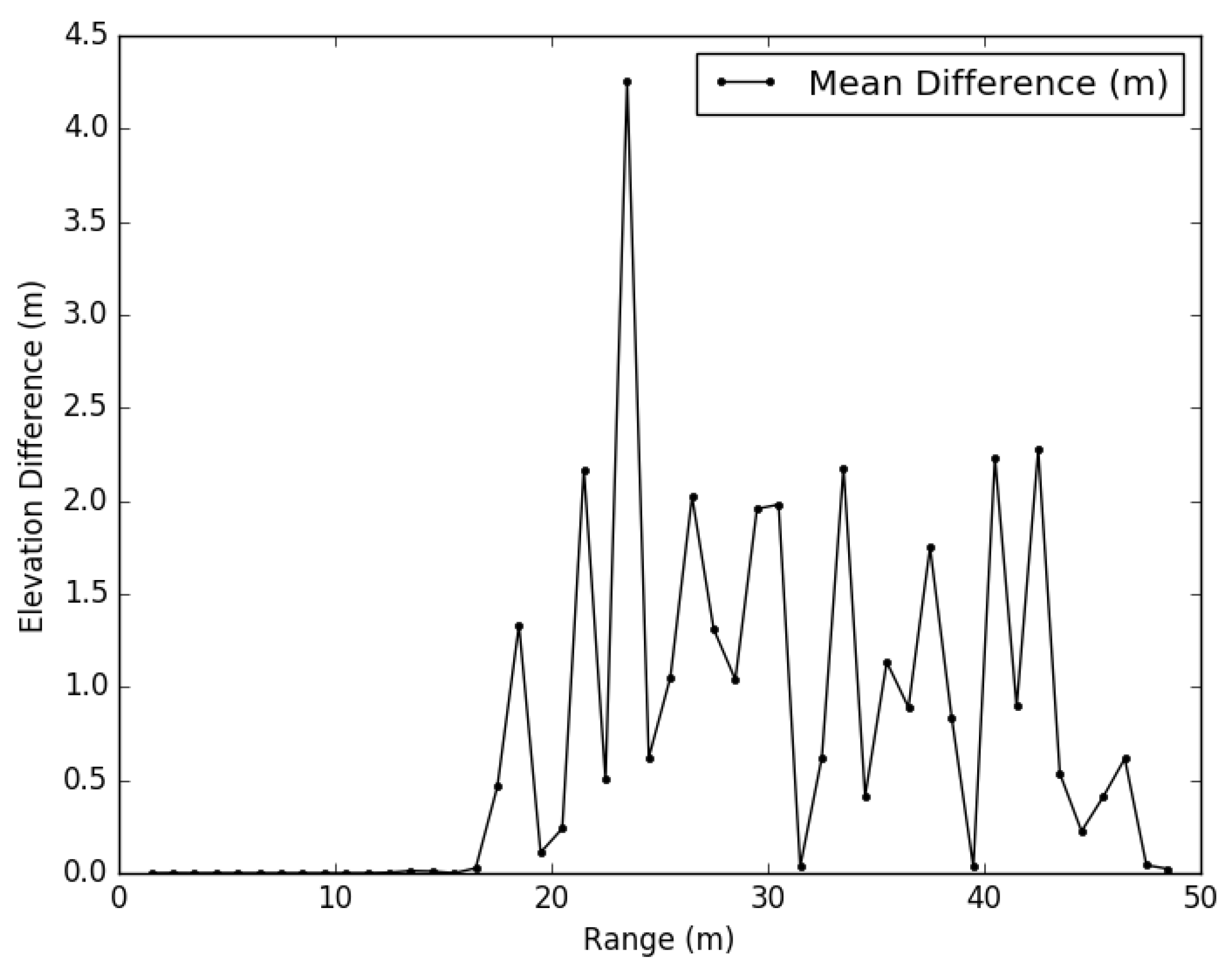
The research presented in this paper shows that even when using a high resolution TLS instrument, in a forest environment, multiple scans are necessary to adequately characterise the DEM surface within a 50-m range from the plot centre. Based on our comparison to ALS data, a multiple scan position survey design with a 25-m radius plot will reduce errors compared to a single scan position design. However, survey time restrictions do not always allow for scan acquisition at multiple scan positions. Our results show that if using a DEM produced from a single scan, it would be advised to limit the range to <25 m from the plot centre.
The mean error for the comparison of the ALS DEM to TS spot heights was 0.15 m, which shows that the airborne LiDAR DEM is consistently above the “true” ground surface. This may be due to dead time for successive ALS measurements not being sufficient, i.e., the laser point return is from grass or understorey, and due to the near nadir view point, the dead time is greater than the distance to the ground, or the inability of the laser to penetrate fully to the ground. The dead time for successive measurements is similar for TLS, but is likely to be less important than for ALS, due to the much larger number of laser returns generated with TLS, increasing the chance that some of them will pass through grass and understorey gaps to hit the ground. Note that RMSE values for comparison of the TLS DEMs to TS spot heights were also all positive, and therefore, the TLS DEMs were also on average above the ground surface measured by the total station, again likely due to the obfuscation of the ground by grass and understorey.
Using a larger grid resolution (i.e., 1 m) to generate the DEM, a simple method such as minimum Z is able to produce a DEM with low error (i.e., 0.19-m mean error for a 1-m grid resolution using a single scan position and at a 25-m plot radius). However, at this resolution, small features in the ground surface are not able to be identified (i.e., they are smaller than 1 m), and so, for use in estimating understorey attributes, it is advised to use a smaller grid resolution and a more complex DEM method such as the one presented here.
The low mean error (0.15 m) from the ALS DEM to TS spot height comparison suggests that where the grid resolution of the ALS DEM fits with the intended forest attributes to be extracted (i.e., the features of interest are not smaller than the ALS grid resolution), then it is appropriate to use the ALS DEM to normalise the TLS point cloud to the height above ground. However, the point density of ALS captures is not always sufficiently high enough to allow a DEM to be produced at the required resolution (often, point density means that the smallest grid resolution possible for an ALS DEM is a 1-m grid resolution). For extracting forest understorey attributes related to features such as coarse woody debris, smaller in size than 1 m, the use of a TLS DEM to normalise point cloud height will be necessary.
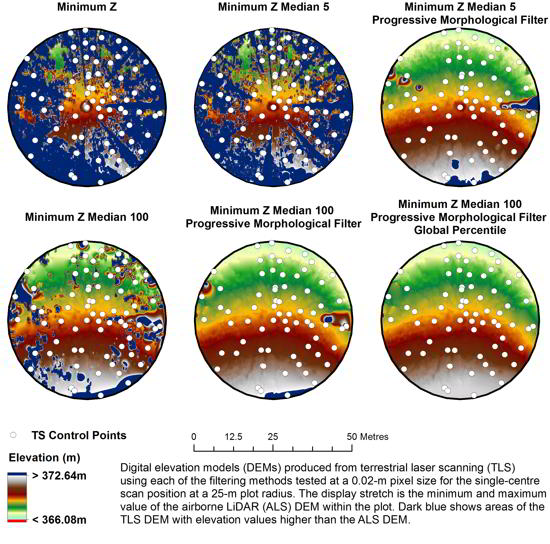
Our results suggest that the practice of using only single and last returns in DEM production from ALS data is not appropriate for TLS data and introduces additional error. The PMF method is routinely used with airborne LiDAR to generate DEMs [15,24]. The results from our analysis show that the combination of a PMF filter with a median filter and global percentile greatly reduces the error of TLS DEMs at smaller grid sizes such as 0.02 m. It is therefore suggested as an important processing step for DEM production from TLS data where a DEM is required at fine grid resolution.
The site we used for our analysis is relatively complex, having areas of varying slope, moderate to high grass cover and a moderate tree density. Using our suggested scan setup of seven scan positions, we were able to produce a DEM with mean error of 0.28 m for a 50-m radius plot under these conditions. This setup should also be appropriate in sites with lower tree density, slope and grass cover. This method however is not designed to be a one fits all solution, but rather to be modified based on plot characteristics, by fine tuning the thresholds and increasing the complexity from the simple minimum Z filter, through to the more complex minimum Z + median 100 + PMF + global percentile method.
Further research is planned to investigate the retrieval of fine-scale understorey attributes from TLS data, including understorey attributes related to point density and average height, as well as the detection of coarse woody debris. For this to be achievable, it was first necessary to derive a robust method of DEM production at a small grid resolution. The literature search conducted did not uncover such a method, and so, the work presented within this paper aims to fill that gap and to provide a general overview of the findings related to TLS DEM production within a forest environment. The lack of understanding of TLS-generated DEM surfaces (or in some cases, the lack of DEM altogether) may influence the accuracy and repeatability of forestry overstorey and understorey attributes produced from TLS data. Accounting for subtle errors is particularly important in monitoring applications, as multiple errors from successive TLS surveys can be compounded and lead to inaccurate results.

5. Conclusions

There are many considerations when producing a DEM from TLS data, and to date, these have not been well understood in the literature (with many methods simply relying on those used for ALS DEM production). Our chosen method presents a protocol for DEM production from TLS data and provides an overview of factors affecting DEMs produced from single and multiple scan positions. In environments with a very low slope, this may not be necessary, and methods such as plane fitting or block point adjustment using the scanner height may suffice. Where comparison against validation data is not possible (due to its unavailability), a simple visual examination of the DEM quality may suffice to identify problems (i.e., overstorey inclusion) and suggest a modified method or threshold adjustment to the user, i.e., introduction of the PMF filter or a global percentile. The method presented here can be accommodated for different environments by progressively adding processing steps, combined with repeated visual or validation data assessment of errors in the output DEMs.

Acknowledgments

We wish to thank Isacc Stiller from the Queensland Department of Natural Resources and Mines (DNRM) for the collection and processing of the total station data at GOLD0101. Furthermore, many thanks to Neil Flood for his help and advice with Python programming. Funding for this research has been provided through the Queensland Government Department of Science, IT and Innovation (DSITI). We would also like to acknowledge DSITI and the Terrestrial Ecosystem Research Network (TERN) Auscover for access and use of the RIEGL VZ400 terrestrial laser scanner.

Author Contributions

Jasmine Muir wrote the paper, devised the analysis methods and analysed the data. Nicholas Goodwin and John Armston designed the original field experiment layout. Stuart Phinn, Nicholas Goodwin, John Armston and Peter Scarth provided input into the contents of the paper, suggestions for analysis and editing of the draft and final versions. Nicholas Goodwin was responsible for the field data collection.

Conflicts of Interest

The authors declare no conflict of interest.

Abbreviations

The following abbreviations are used in this manuscript:
ALSAirborne Laser Scanning
AHDAustralian Height Datum
BABasal Area
DBHDiameter at Breast Height
DEMDigital Elevation Model
IDWInverse Distance Weighting
IMUInertial Measurement Unit
PAIPlant Area Index
PCPPermanent Control Point
PMFProgressive Morphological Filter
PSMPermanent Survey Marks
QEHAQueensland Ellipsoidal Height Adjustment
RMSERoot Mean Squared Error
TINTriangulated Irregular Network
TLSTerrestrial Laser Scanning
TSTotal Station

References

  1. Asner, G.P.; Owen-Smith, N.; Loarie, S.R.; Davies, A.B.; Le Roux, E.; Levick, S.R. Habitat differences do not explain population declines of sable antelope in an African savanna: Vegetation structure and sable habitat use. J. Zool. 2015, 297, 225–234. [Google Scholar] [CrossRef]
  2. Danson, F.M.; Morsdorf, F.; Koetz, B. Airborne and terrestrial laser scanning for measuring vegetation canopy structure. In Laser Scanning for the Environmental Sciences; Heritage, G.L., Large, A.R.G., Charlton, M., Eds.; Blackwell Pub.: Chichester, UK, 2009. [Google Scholar]
  3. Liang, X.; Kankare, V.; Hyyppä, J.; Wang, Y.; Kukko, A.; Haggrén, H.; Yu, X.; Kaartinen, H.; Jaakkola, A.; Guan, F.; et al. Terrestrial laser scanning in forest inventories. ISPRS J. Photogramm. Remote Sens. 2016, 115, 63–77. [Google Scholar] [CrossRef]
  4. Van Leeuwen, M.; Nieuwenhuis, M. Retrieval of forest structural parameters using LiDAR remote sensing. Eur. J. For. Res. 2010, 129, 749–770. [Google Scholar] [CrossRef]
  5. Zhao, F.; Yang, X.; Schull, M.A.; Román-Colón, M.O.; Yao, T.; Wang, Z.; Zhang, Q.; Jupp, D.L.; Lovell, J.L.; Culvenor, D.S.; et al. Measuring effective leaf area index, foliage profile, and stand height in New England forest stands using a full-waveform ground-based LiDAR. Remote Sens. Environ. 2011, 115, 2954–2964. [Google Scholar] [CrossRef]
  6. Beland, M.; Baldocchi, D.D.; Widlowski, J.L.; Fournier, R.A.; Verstraete, M.M. On seeing the wood from the leaves and the role of voxel size in determining leaf area distribution of forests with terrestrial LiDAR. Agric. For. Meteorol. 2014, 184, 82–97. [Google Scholar] [CrossRef]
  7. Calders, K.; Newnham, G.; Burt, A.; Murphy, S.; Raumonen, P.; Herold, M.; Culvenor, D.; Avitabile, V.; Disney, M.; Armston, J.; et al. Nondestructive estimates of above-ground biomass using terrestrial laser scanning. Methods Ecol. Evol. 2015, 6, 198–208. [Google Scholar] [CrossRef]
  8. Zhao, K.; Popescu, S.; Nelson, R. Lidar remote sensing of forest biomass: A scale-invariant estimation approach using airborne lasers. Remote Sens. Environ. 2009, 113, 182–196. [Google Scholar] [CrossRef]
  9. Calders, K.; Schenkels, T.; Bartholomeus, H.; Armston, J.; Verbesselt, J.; Herold, M. Monitoring spring phenology with high temporal resolution terrestrial LiDAR measurements. Agric. For. Meteorol. 2015, 203, 158–168. [Google Scholar] [CrossRef]
  10. Eitel, J.U.; Höfle, B.; Vierling, L.A.; Abellán, A.; Asner, G.P.; Deems, J.S.; Glennie, C.L.; Joerg, P.C.; LeWinter, A.L.; Magney, T.S.; et al. Beyond 3-D: The new spectrum of LiDAR applications for earth and ecological sciences. Remote Sens. Environ. 2016, 186, 372–392. [Google Scholar] [CrossRef]
  11. Goodwin, N.R.; Armston, J.D.; Muir, J.; Stiller, I. Monitoring gully change: A comparison of airborne and terrestrial laser scanning using a case study from Aratula, Queensland. Geomorphology 2017, 282, 195–208. [Google Scholar] [CrossRef]
  12. Paynter, I.; Saenz, E.; Genest, D.; Peri, F.; Erb, A.; Li, Z.; Wiggin, K.; Muir, J.; Raumonen, P.; Schaaf, E.S.; et al. Observing ecosystems with lightweight, rapid-scanning terrestrial LiDAR scanners. Remote Sens. Ecol. Conserv. 2016, 2, 174–189. [Google Scholar] [CrossRef]
  13. Calders, K.; Armston, J.; Newnham, G.; Herold, M.; Goodwin, N. Implications of sensor configuration and topography on vertical plant profiles derived from terrestrial LiDAR. Agric. For. Meteorol. 2014, 194, 104–117. [Google Scholar] [CrossRef]
  14. Bater, C.W.; Coops, N.C. Evaluating error associated with LiDAR-derived DEM interpolation. Comput. Geosci. 2009, 35, 289–300. [Google Scholar] [CrossRef]
  15. Goodwin, N.R.; Armston, J.; Stiller, I.; Muir, J. Assessing the repeatability of terrestrial laser scanning for monitoring gully topography: A case study from Aratula, Queensland, Australia. Geomorphology 2016, 262, 24–36. [Google Scholar] [CrossRef]
  16. Heritage, G.L.; Milan, D.J.; Large, A.R.; Fuller, I.C. Influence of survey strategy and interpolation model on DEM quality. Geomorphology 2009, 112, 334–344. [Google Scholar] [CrossRef]
  17. Meng, X.; Currit, N.; Zhao, K. Ground Filtering Algorithms for Airborne LiDAR Data: A Review of Critical Issues. Remote Sens. 2010, 2, 833–860. [Google Scholar] [CrossRef]
  18. Fan, L.; Atkinson, P.M. Accuracy of Digital Elevation Models Derived From Terrestrial Laser Scanning Data. IEEE Geosci. Remote Sens. Lett. 2015, 12, 1923–1927. [Google Scholar] [CrossRef]
  19. Mongus, D.; Žalik, B. Parameter-free ground filtering of LiDAR data for automatic DTM generation. ISPRS J. Photogramm. Remote Sens. 2012, 67, 1–12. [Google Scholar] [CrossRef]
  20. Moskal, L.M.; Zheng, G. Retrieving Forest Inventory Variables with Terrestrial Laser Scanning (TLS) in Urban Heterogeneous Forest. Remote Sens. 2011, 4, 1–20. [Google Scholar] [CrossRef]
  21. Puttonen, E.; Krooks, A.; Kaartinen, H.; Kaasalainen, S. Ground Level Determination in Forested Environment with Utilization of a Scanner-Centered Terrestrial Laser Scanning Configuration. IEEE Geosci. Remote Sens. Lett. 2015, 12, 616–620. [Google Scholar] [CrossRef]
  22. Liang, X.; Hyyppä, J. Automatic Stem Mapping by Merging Several Terrestrial Laser Scans at the Feature and Decision Levels. Sensors 2013, 13, 1614–1634. [Google Scholar] [CrossRef] [PubMed]
  23. Yang, X.; Strahler, A.H.; Schaaf, C.B.; Jupp, D.L.; Yao, T.; Zhao, F.; Wang, Z.; Culvenor, D.S.; Newnham, G.J.; Lovell, J.L.; et al. Three-dimensional forest reconstruction and structural parameter retrievals using a terrestrial full-waveform LiDAR instrument (Echidna®). Remote Sens. Environ. 2013, 135, 36–51. [Google Scholar] [CrossRef]
  24. Pirotti, F.; Guarnieri, A.; Vettore, A. Ground filtering and vegetation mapping using multi-return terrestrial laser scanning. ISPRS J. Photogramm. Remote Sens. 2013, 76, 56–63. [Google Scholar] [CrossRef]
  25. Zhang, K.; Chen, S.C.; Whitman, D.; Shyu, M.L.; Yan, J.; Zhang, C. A progressive morphological filter for removing nonground measurements from airborne LIDAR data. IEEE Trans. Geosci. Remote Sens. 2003, 41, 872–882. [Google Scholar] [CrossRef]
  26. Axelsson, P. Processing of laser scanner data—Algorithms and applications. ISPRS J. Photogramm. Remote Sens. 1999, 54, 138–147. [Google Scholar] [CrossRef]
  27. Heritage, G.L.; Large, A.R.G.; Charlton, M. Laser Scanning for the Environmental Sciences; Blackwell Pub.: Chichester, UK, 2009. [Google Scholar]
  28. Chaplot, V.; Darboux, F.; Bourennane, H.; Leguédois, S.; Silvera, N.; Phachomphon, K. Accuracy of interpolation techniques for the derivation of digital elevation models in relation to landform types and data density. Geomorphology 2006, 77, 126–141. [Google Scholar] [CrossRef]
  29. Li, J.; Heap, A.D. A Review of Spatial Interpolation Methods for Environmental Scientists; Geoscience Australia: Canberra, Australia, 2008.
  30. Fleming, M.D.; Hoffer, R.M. Machine Processing of Landsat MSS Data and DMA Topographic Data for Forest Cover Type Mapping. 1979. Available online: http://docs.lib.purdue.edu/ cgi/viewcontent.cgi? article=1079&context=larstech (accessed on 14 August 2017).
  31. Muir, J.; Schmidt, M.; Tindall, D.; Trevithick, R.; Scarth, P.; Stewart, J.B. Field Measurement of Fractional Ground Cover: A Technical Handbook Supporting Ground Cover Monitoring for Australia; Technical Report; ABARES: Canberra, Australia, 2011.
Figure 1. GOLD0101 site location (top left), photo of the study site (top right), DEM (bottom left) and slope (bottom right) derived from ALS captured in 2014. A white circle shows the 25-m radius from the centre TLS scan position (Scan Position 1).
Remotesensing 09 00843 g001aRemotesensing 09 00843 g001b
Figure 2. Position of reflective targets used in Scan Position 1 (centre scan) registration (red cross on white circle) and permanent control points (PCPs) used for registration of scans to real-world coordinates (blue circle) for the 27 November 2015 TLS data acquisition. The location of all seven scan positions is shown in Figure 1.
Remotesensing 09 00843 g002
Figure 3. Position of virtual transects used to test the effect of range on the elevation difference between the filtered minimum Z images produced from all returns and single/last returns at a 0.2-m grid resolution for the single-centre scan (Scan Position 1). The outer circle is the 50-m plot radius, and the inner circle is the 25-m plot radius.
Remotesensing 09 00843 g003
Figure 4. DEMs produced using the minimum Z value for each of the grid resolutions tested for the single-centre scan position at a 25-m plot radius. The display stretch is the minimum and maximum value of the airborne LiDAR DEM within the plot. Dark blue shows areas of the TLS DEM with elevation values higher than the ALS DEM.
Remotesensing 09 00843 g004
Figure 5. Mean elevation difference of the filtered elevation values (0.2-m grid resolution) for all returns and only single/last returns (single/last returns—all returns) binned at 1-m intervals of range from the scan origin for centre Scan Position 1.
Remotesensing 09 00843 g005
Figure 6. Mean residual error (m) of TS spot heights for different methods of generating DEMs from the single-centre scan at a 25-m plot radius (n = 71).
Remotesensing 09 00843 g006
Figure 7. DEMs produced using each of the filtering methods tested at a 0.02-m pixel size, for the single-centre scan position, at a 25-m plot radius. The display stretch is the minimum and maximum value of the airborne LiDAR DEM within the plot. Dark blue shows areas of the TLS DEM with elevation values higher than the ALS DEM.
Remotesensing 09 00843 g007
Figure 8. Difference between the single-centre scan, four scan positions (1, 2, 4, 6) and all scan positions, for the 2014 ALS dataset (1-m pixel resolution) at a 25-m range (inner circle) and a 50-m (outer circle) range from the plot centre. Note that there was too much space between ground points at 0.02-m resolution for the interpolation to work across the entire area of the 25 m–50 m plot radius for the single-centre scan (Scan Position 1).
Remotesensing 09 00843 g008
Table 1. Selected citations on DEMs derived from terrestrial laser scanning data.
Ref.FilterInterpolationNo. of ScansPixel SizePlot SizeError Stat.
[13]Last returnsLinear Plane1, 4, 51–8 m 50 × 50 m0.5–0.6 m
Minimum ZFittingRMSE
[15]Minimum ZTriangulated <0.05 m mean error
Median 3 × 3 Irregular240.02–0.5 m> 100 × 100 m
1st and allNetwork (TIN)
[21]RadialSpline Height6radius dependent25 m radius0.2–0.3 m RMSE
Binning
Slope
[22]Minimum ZNone4N/A10 m radiusN/A
[23]Minimum ZIn-painting5, 90.5 m 50 × 50 mN/A
RANSAC
[24]Single andN/A10.1 m> 100 × 100 m0.227–0.411 m *
Last ReturnsRMSE
Intensity−0.003–0.134 m
Morphologicalmean error
ALS validation dataset; TS validation dataset; * TLS point cloud-derived validation dataset.
Table 2. RMSE and number of reflectors used for registration of each scan position from the 27 November 2015 survey. The location of scan positions is shown in Figure 1.
Scan PositionNo. of ReflectorsRMSE (m)
1300.000
2150.007
3110.012
4160.014
5180.016
6180.012
7170.015
Table 3. Comparison of error statistics (mean, standard deviation of errors (SD), minimum (Min), maximum (Max) and root mean squared error (RMSE) for DEMs generated using minimum Z values from all returns for the 25-m plot radius (TS spot heights n = 71) and the 50-m plot radius (TS spot heights n = 171 for grid resolutions ≥0.05 m and n = 158 for the 0.02-m grid resolution) from the centre scan position (Scan Position 1) at all tested grid resolutions.
Pixel Size (m)Plot Radius (m)Mean (m)SD (m)Min (m)Max (m)RMSE (m)
0.02255.805.510.0918.118.00
0.05254.165.120.0818.896.60
0.10252.453.580.0717.954.34
0.20250.821.840.0711.552.02
0.50250.300.540.054.660.62
1.00250.190.100.000.560.22
0.02508.746.260.0924.7910.75
0.05507.946.750.0824.7110.42
0.10505.945.910.0722.678.38
0.20504.055.400.0722.196.75
0.50501.572.900.0514.233.30
1.00500.631.230.0010.871.38
Table 4. Comparison of error statistics for the single-centre scan (Scan Position 1) using all returns, only single/last returns and all returns plus a deviation threshold (deviation < 10) for the 25-m and 50-m plot radii. All DEMs were produced at a 0.2-m grid resolution.
Plot Radius (m)DEMMean (m)SD (m)Min (m)Max (m)RMSE (m)No. of Points
25All Returns0.821.840.0711.552.0271
25Single/Last Returns0.952.210.0712.652.4171
25All Returns Deviation0.821.840.0711.552.0271
50All Returns4.055.400.0722.196.75171
50Single/Last Returns5.805.740.1022.888.14171
50All Returns Deviation4.055.400.0722.196.75171
Table 5. Method: minimum Z + median 100 + PMF + global percentile. Comparison of the error statistics for the DEM filtering method at the 25-m plot radius (TS spot heights n = 71) and the 50-m plot radius (TS spot heights n = 171 for grid resolutions ≥0.05 m and n = 158 for 0.02-m grid resolution), for the single-centre scan (Scan Position 1) at all tested grid resolutions.
Plot Radius (m)Pixel Size (m)Mean (m)SD (m)Min (m)Max (m)RMSE (m)
Single Scan250.020.310.150.000.920.34
0.050.310.140.070.740.34
0.100.270.120.060.580.30
0.200.250.120.070.580.28
0.500.220.110.050.580.25
1.000.190.100.000.560.21
500.020.620.780.005.690.99
0.050.991.510.0710.641.80
0.100.861.330.069.461.58
0.200.540.500.073.520.73
0.500.440.32−0.341.430.54
1.000.380.36−1.261.330.52
Table 6. Method: minimum Z all returns. Comparison of error statistics for the DEM filtering method at the 25-m plot radius (TS spot heights n = 71) and the 50-m plot radius (TS spot heights n = 171) at all tested grid resolutions produced from the point cloud from the four scan positions (Scan Positions 1, 2, 4 and 6) and from the combined point cloud from all seven scan positions. Error statistics for the single-centre scan position using the minimum Z all returns method are shown in Table 3.
Plot Radius (m)Pixel Size (m)Mean (m)SD (m)Min (m)Max (m)RMSE (m)
Four Scans250.025.264.440.0716.536.88
0.052.823.620.0714.034.59
0.101.462.500.0710.812.90
0.200.481.160.077.701.26
0.500.200.120.050.780.23
1.000.170.070.000.390.18
500.026.565.450.0721.858.53
0.054.635.440.0728.787.15
0.103.154.730.0727.485.69
0.201.563.510.0724.023.84
0.500.380.940.029.911.02
1.000.220.150.001.130.27
All Scans250.024.684.040.0716.276.18
0.051.932.650.0713.293.28
0.100.892.020.0710.552.21
0.200.340.930.077.850.99
0.500.170.070.050.390.18
1.000.150.060.000.350.16
500.024.924.840.0321.016.90
0.052.553.660.0318.714.46
0.101.412.950.0217.653.27
0.200.531.550.0313.451.64
0.500.180.100.010.570.21
1.000.160.070.000.420.17
Table 7. Method: minimum Z + median 100 + PMF + global percentile. Comparison of error statistics for DEM filtering method at the 25-m plot radius (TS spot heights n = 71) and the 50-m plot radius (TS spot heights n = 171) for DEMs at all tested grid resolutions from the combined point cloud from all seven scan positions. Error statistics for the single-centre scan position using the minimum Z + median 100 + PMF + global percentile method are shown in Table 5.
Plot Radius (m)Pixel Size (m)Mean (m)SD (m)Min (m)Max (m)RMSE (m)
All Scans250.020.280.110.080.680.30
0.050.310.380.073.180.49
0.100.260.250.072.090.36
0.200.190.090.070.480.21
0.500.170.070.050.390.18
1.000.150.060.000.350.17
500.020.280.110.030.680.30
0.050.290.280.023.180.41
0.100.250.190.022.090.31
0.200.200.100.030.500.23
0.500.180.090.010.510.20
1.000.160.070.000.420.17
Table 8. Comparison of TS spot heights to ALS 1-m grid resolution DEM.
Mean (m)SD (m)Min (m)Max (m)RMSE (m)
TS Spot Heights0.150.10−0.160.440.18
Table 9. Comparison of the error statistics for DEMs produced from TLS surveys on three different dates, at a 25-m and a 50-m range from the plot centre, using all scan positions with a 0.2-m grid resolution and the minimum Z + median 100 + PMF + global percentile method. TS spot heights n = 71 for a plot radius of 25 m and n = 171 at a plot radius of 50 m.
Range (m)Error Statistic25 November 201527 November 20159 February 2017
25Mean Error (m)0.220.190.16
SD (m)0.090.090.08
RMSE (m)0.240.210.18
50Mean Error (m)0.220.200.15
SD (m)0.100.100.09
RMSE (m)0.240.230.17

