
Extension of a Fast GLRT Algorithm to 5D SAR Tomography of Urban Areas


Dipartimento di Ingegneria, Università degli Studi di Napoli “Parthenope”, Naples 80143, Italy
*
Author to whom correspondence should be addressed.
Remote Sens. 2017, 9(8), 844; https://0-doi-org.brum.beds.ac.uk/10.3390/rs9080844
Submission received: 12 June 2017
/
Revised: 26 July 2017
/
Accepted: 4 August 2017
/
Published: 14 August 2017
Abstract
:This paper analyzes a method for Synthetic Aperture Radar (SAR) Tomographic (TomoSAR) imaging, allowing the detection of multiple scatterers that can exhibit time deformation and thermal dilation by using a CFAR (Constant False Alarm Rate) approach. In the last decade, several methods for TomoSAR have been proposed. The objective of this paper is to present the results obtained on high resolution tomographic SAR data of urban areas, by using a statistical test for detecting multiple scatterers that takes into account phase variations due to possible deformations and/or thermal dilation. The test can be evaluated in terms of probability of detection (PD) and probability of false alarm (PFA), and is based on an approximation of a Generalized Likelihood Ratio Test (GLRT), denoted as Fast-Sup-GLRT. It was already applied and validated by the authors in the 3D case, while here it is extended and experimented in the 5D case. Numerical experiments on simulated and on StripMap TerraSAR-X (TSX) data have been carried out. The presented results show that the adopted method allows the detection of a large number of scatterers and the estimation of their position with a good accuracy, and that the consideration of the thermal dilation and surface deformation helps in recovering more single and double scatterers, with respect to the case in which these contributions are not taken into account. Moreover, the capability of method to provide reliable estimates of the deformations in urban structure suggests its use in structure stress monitoring.
1. Introduction
Multi-channel Synthetic Aperture Radar (SAR) interferometry allows accurate reconstructions of the height profile of the observed scenes [1,2,3]. Spaceborne differential interferometric SAR (DInSAR) [4] involves the exploitation of multiple interferograms computed from pairs of complex SAR images and aims at measuring surface deformations. This technique evolved in the last three decades since its first appearance. Among the different proposed methods for surface deformation measurement and monitoring, based on the exploitation of SAR images, the Permanent Scatterers (PS) techniques have been shown to be effective and largely applied. They make use of a stack of SAR images, are essentially phase-only model based, and mostly assume the presence of only one dominant scatterer per resolution cell [5,6,7,8,9,10,11,12,13,14]. Recently, the introduction of new sensors in X-Band, such as TerraSAR-X (TSX) and the Italian COSMO-SkyMed (CSK) constellation, have stimulated this research field since the very small wavelength (~3.1 cm) allows for measuring small surface displacements, even those caused by thermal dilation of the imaged targets, which affects the phase signature [6]. In fact, in [7,8,9,10], a Permanent Scatterers Inteferometry (PSI) technique based on an extended phase model has been shown to be capable of separating the thermal expansion from the total observed deformation, thus providing the map of the thermal expansion parameter. Anyway, conventional PSI techniques consider the case of single point-wise scatterers exhibiting a high temporal coherence in each range-azimuth resolution cell. More recently, extended PSI approaches have been introduced for considering distributed scatterers [11] and partially coherent scatterers [12] for increasing the density of measurement points over non-urban areas. Moreover, models involving higher order statistics, in order to allow two or more scattering centers within the same resolution cell, have been introduced [13].
The main limitation of PS approaches is the assumption of only single scatterers in the resolution cell that does not allow for properly treating the layover problem, which severely affects the urban areas. The presence of multiples scatterers interfering in the same resolution cell may impair the method’s performance, and misdetections of persistent scatterers and inaccuracies in height velocity and time series measurements may occur.
In SAR tomography (TomoSAR) [14], the use of a stack of complex-valued images makes possible the separation of the scatterers interfering within the same range-azimuth resolution cell, by synthesizing apertures along the elevation direction and achieving elevation resolution, so as to provide the full 3D scene reflectivity profile along azimuth, range, elevation, and also along average velocity deformation [15]. TomoSAR consists of resolving an inversion problem. Different estimators, such Singular Value Decomposition (SVD) [16], and Compressive Sensing (CS) [17,18,19,20], have been proposed, showing the good capability of TomoSAR of obtaining accurate 3D building reconstructions [21,22]. In [23,24], the possibility of combining SAR tomography with a PSI approach, toward the objective of improving deformation sampling in layover-affected urban areas, has been investigated.
One of the main issues to be faced in TomoSAR techniques is the presence of outliers that limits the accuracy in extracting true scatterers. For selecting the most reliable scatterers and reducing the outliers occurrence, scatterers detection can be framed in the more general context of adaptive radar detection of targets embedded in Gaussian noise, which can be addressed using the techniques of statistical hypothesis testing [25]. This is a very active research field, which has been an object of great interest in the last decades. A comprehensive and systematic analysis of composite hypothesis testing and of the detectors design criteria, including Generalized Likelihood Ratio Test (GLRT), can be found in [26,27]. In SAR Tomography, a sequential GLRT [28], allowing for discriminating between single and double scatterers and to estimate their intensity and elevation, has been recently introduced. This approach has been also extended to allow the simultaneous retrieval of scatterer elevation and deformation parameters [29,30,31], showing that X-Band is particularly effective in estimating the thermal dilation contribution. Anyway, this method does not exhibit good performance when trying to super resolve close scatterers.
In [32], an alternative implementation of the GLRT approach, denoted as Sup-GLRT, has been analyzed. It is based on the exploitation of the sparsity assumption and on the search of the signal support (i.e., the positions of the non-zero samples in the unknown sparse vector) that best matches the data. This statistical test exploits a nonlinear maximization for detecting at most Kmax different scatterers in the same azimuth-range resolution cell and for estimating their elevation. In principle, this approach allows improved spatial and radiometric resolutions, since it is based on nonlinear processing. Moreover, it permits evaluating detection performance in terms of probability of detection achievable with a given number of measurements and signal-to-noise ratio, and probability of false alarm (PFA), which can be fixed to an assigned value. Then, by imposing a small value of PFA, the outliers’ occurrence can be noticeably reduced.
In [33], a similar sequential approach has been proposed—the parametric multi-look relaxation (M-RELAX) algorithm used to recover multiple backscattering sources mapped into the same resolution cell. It is a spectral estimation technique, which follows a different approach from the Sup-GLRT detector. The main difference between the two approaches is related to the search stop criterion: in [33], the search terminates when a convergence, based on a properly defined cost function, has been reached, while, in Sup-GLRT, the search terminates when the generalized likelihood ratio is below a threshold that is evaluated fixing a false alarm probability.
A drawback of Sup-GLRT is that numerical complexity increases very rapidly with the size of the unknown vector. This issue is of fundamental importance for the extension of the method to the four-dimensional (4D) case [15], where the estimation of the deformation velocity is added, or to the five-dimensional (5D) case, where the estimation of the thermal dilation is considered along with the deformation velocity [28]. Recently, in [34], an approximated version of Sup-GLRT, denoted Fast-Sup-GLRT, has been presented. The approximation introduced allows to drastically reduce the computational cost, which for Sup-GLRT is increasing with a combinatorial trend [32] alongside the size N of the unknown vector, while a trend which is linear with N is obtained by using Fast-Sup-GLRT. In [34], the method has been introduced and analyzed only for the 3D case, while its practicability for the 4D and 5D cases has not been addressed.
In this paper, we extend the tomographic detection approach followed by the Fast-Sup-GLRT to the 5D case, in order to obtain 5D reconstructions of the illuminated scenes. 5D tomographic processing is based on the use of an extended phase model having a strong impact on the size of the unknown reflectivity vector, which becomes very large; for this reason, the practical application of a statistical detection approach to 5D SAR tomography fully benefits from the approximation introduced by the Fast-Sup-GLRT detector. Anyway, an important issue that has to be investigated to state its applicability to 5D SAR tomography is the evaluation of the probability of detection achievable with a given probability of false alarm and of the estimation accuracy for height, deformation velocity and thermal dilation, in the case of the extended phase model.
The extended phase model and the approximated procedure for the search of the positions of the non-zero samples in the unknown sparse vector that best match the data are briefly reviewed in Section 2. In Section 3, results on simulated and real data are presented to validate and substantiate the proposed approach. It is shown, both on simulated and real data, the need of taking into account the extended phase model in order to detect scatterers affected by time deformation. Moreover, by means of an appropriate analysis, it is shown that keeping the probability of a false alarm to a constant and low value allows the selection of the scatterers providing reliable height and deformation estimates. High-resolution SAR data have been considered, in order to highlight the need for a method able to separate multiple scatterers. In fact, with this kind of data, the interference between scatterers on the ground and on buildings (façade and roof) is more frequent and the layover problem is more severe. StripMap TSX (provided by DLR German Space Centre) data have been used.
2. Tomographic Signal and 5D Scatterer Detection
Let us assume to have a stack of M SAR interferometric images of the same scene, acquired at different times tn and with different orthogonal baselines with respect to a reference acquisition. The images are properly registered, with a sub-pixel accuracy, and preprocessed to remove flat Earth interferometric phase [35] and to depurate the focused images from the atmospheric and nonlinear deformation contributions on a small scale (low resolution) [31]. Then, in any range-azimuth pixel, the m-th acquired image um is given by the superposition of the signal backscattered by the targets located at the given azimuth and range coordinates, and at different elevation s. Then, the image signal, in the case of slow moving scatterers, can be expressed by [31]:
where λ is the operating wavelength, the distance between the image pixel and the reference antenna, S1 the extension of the observed scene along elevation, and d(s,tm) is the deformation of the scatterer at the elevation s and at the time tm, which is typically related to subsidence or geophysical phenomena.
With the advent of the last generation SAR sensors, working at higher frequency, such as CSK and TSX/TDX working at X-Band, the model of the deformation signal d(s,tm) has been extended by including minute deformation components, such as thermal dilation.
This is a direct consequence of the reduction of the wavelength that allows a higher phase sensitivity to range variations.
Then, the model adopted for the deformation signal is typically assumed to be composed of linear and nonlinear contributions [31]:
where Tm is the temperature of the scene at the time tm, v0(s) is the velocity of the slow linear deformation, having the dimension of (m/s), and k0(s) is a thermal coefficient, having the dimension of (m/°C), of the scatterer at elevation s, representing the phase-to temperature sensitivity and depending upon material and/or physical structure.
d(s, tm,Tm) = v0(s)tm + k0(s)Tm + dNL(s, tm, Tm),
We consider now the term and express it through the 2D Fourier transform:
computed in the temporal and thermal frequencies 2tm/λ and 2Tm/λ. We note that if the nonlinear deformation dNL(s, tm, Tm) is small respect to λ, is a peaked function, with a peak in the origin of the v-k plane. Substituting (2) and (3) in (1), and neglecting the integration volume changes with respect to small shifts of integration variables, it is obtained:
where V1 and K1 are the range of values of v and k, and , with the function with a peak in the point . In the ideal case of the absence of nonlinear deformations, the function g tends to a two-dimensional Dirac delta function of the two variable v and k, located in the point of coordinates . Then, the unknown elevation reflectivity profile can be derived from by sampling it in the values of v and k, for which assumes its maximum value. The function , in principle, can be obtained from the acquired data by inverting the 3D Fourier transform (4).
The discrete version of the signal Model (4) is obtained by discretizing s, v and k with steps ∆s = ρs/ηs, ∆v = ρv/ηv and ∆k = ρk/ηk with ηs, ηv and ηk oversampling factors (greater than or equal to one) and ρs, ρv and ρk the Rayleigh resolutions given by:
with SB, tB and TB the overall baseline, time and temperature spans of the measured data, respectively. After discretization, Equation (4) becomes:
Equation (5) expresses a Discrete Fourier Transform (DFT) relation between the data u and the unknown . Therefore, in principle, the problem of reconstructing the scatterers located at different elevations and with deformation velocities and thermal dilation, even interfering in the same azimuth-range resolution cell, can be performed by means of an inverse 3D DFT. This procedure, however, would require the image acquisition in a fine grid of points uniform with respect to the baselines s’, the acquisition time t and the temperature T. This requirement is not met in practical applications, where the number of measurements is much lower than the one required. Moreover, they are not uniformly spaced. Then, alternative techniques have to be used.
Equation (5) can be written in matrix form, introducing the N × 1 column vector γ whose elements are the samples computed in all the triplets (i,l,n), with i = 1, …, Ns, l = 1, …, Nv, n = 1, …, Nk, and N = NsNvNk, and the M × 1 data vector u collecting the measurements , with m = 1, …, M, so that:
where w is an M × 1 vector representing noise and clutter, and Φ is an M × N measurement matrix, whose m-th row φm is given by vec(Φm3), where vec is the operator transforming a three-dimensional matrix of size Ns × Nv × Nk in a row vector of size N = NsNvNk. By loading in the vector all the elements of the matrix scanned in a preassigned order, and Φm3 is the three-dimensional matrix of size Ns × Nv × Nk, whose element of entries (i,l,n) is given by:
We note that the number of columns N = Ns × Nv × Nk of the matrix Φ depend on the grid used for the discretization (6).
Due to the impulsive behavior of respect to v and k, we can observe that, for a fixed value of s, only one element of γ, corresponding to a single value of the couple (v,k), will be different from zero. Then, many elements of the vector γ will be equal to zero. Moreover, when the observed scene is an urban area or a scarcely vegetated area, the discretized elevation profile can be assumed to be sparse along s, since only a few scatterers can be present in the same azimuth–range resolution cell. In this case, we can assume that, at most, Kmax scatterers are present in the same range-azimuth resolution cell, and the detection problem can be formulated in terms of the following Kmax + 1 statistical hypotheses [32]:
Hi: presence of i scatterers, with i = 0, …, Kmax.
For deciding which statistical hypothesis is verified, a statistical multiple hypothesis GLRT test [36] can be used. This approach has the advantage of enabling the test performance in terms of probabilities of false alarms, of detection and of false detection.
As far as the statistical model of (6) is concerned, the noise vector w can be assumed as circularly symmetric complex (or proper complex) Gaussian vector, with uncorrelated samples and mutually uncorrelated real and imaginary parts, with zero-mean and same variance . When the scatterers are absent (hypothesis H0), u is a circularly symmetric Gaussian random vector with zero-mean and covariance matrix , with I the identity matrix, while, when i scatterers are present (hypothesis Hi), u is a circularly symmetric Gaussian random vector, with the same covariance matrix and mean , with γ an i-sparse vector [32] with support . In this assumption, we notice that , where and are the M × i matrix and the I × 1 vector obtained by extracting from and the i columns and the i samples, respectively, corresponding to the positions of the non-zero elements in . Then, the joint statistical distribution of the data vector u in the statistical hypothesis Hi can be written as:
where the noise variance , the vector γ and its support Ωi are unknown. Then, a sequential sub-optimal GLRT test, based on Kmax steps, can be applied. At each step i + 1, with i = 0, …, Kmax − 1, the following statistical binary hypothesis test, devoted to decide for the presence i scatterers (hypothesis Hi) or for the presence of more than i scatterers (hypothesis HK>i), is applied:
By deriving the Maximum Likelihood (ML) estimates of and in closed form and substituting it in (10), at each step I + 1, the following binary hypothesis test, denoted as Sup-GLRT, is obtained [32]:
where is the support of cardinality i (i.e., the positions of the i elements different from zero in the vector γ) minimizing the term , where , with H denoting the Hermitian and a matrix of size M × i obtained by extracting from only the i columns of index l1, l2, …, li, corresponding to the signal support. For i = 0, it results as , since = Ø.
We notice that, the test (11) applied at each i+1 step, is equivalent to performing a model order selection between the models of order i and those of order Kmax. This problem is discussed in [37], where it is shown that a natural implementation of the GLRT with a specific threshold can be considered equivalent to the model order selection approach based on the Information Criterion (IC) rule.
From (11), it is evident that Sup-GLRT involves at each step i + 1 an i-dimensional search of the support maximizing the numerator, besides to the Kmax-dimensional minimization of the denominator, which is common to all the steps of the sequential test, and can be performed only once. It can be easily shown that the computational complexity increases with a combinatorial trend with the size N of the vector γ.
To reduce computational complexity, the i-dimensional search of the generic support can be performed by minimizing the term through i iterative minimizations based on a one-dimensional exhaustive search over i supports of cardinality one. The sequential GLRT test based on this approximated minimization is denoted as Fast-Sup-GLRT and has been analyzed in detail in [34]. It can be easily shown that the computational cost of the minimization procedure is linear with N [34].
For better explaining the adopted minimization approach, we assume that we want to detect the presence of two scatterers (i.e., Kmax = 2). Then, we have to search for the support of cardinality 2, i.e., the positions of the two non-zero elements in the unknown reflectivity vector, which best matches the data. The Fast-Sup-GLRT detector performs this search in the following way: first, the position l1 of the most significant element in the unknown vector is searched for (among all the possible N positions) by minimizing with respect to l the term where, and l = 1, …, N; then, after fixing the position of the first scatterer to l1, the search of the second position l2 (among the remaining N − 1 positions) is performed by minimizing with respect to l the term where and l = 1,…, l1 − 1, l1 + 1,…, N.
In order to give an intuitive explanation of how the algorithm works in the case Kmax = 2, we suppose that the two scatterers are perfectly estimated and that the maximization over the support is done without any approximation. The algorithm has two steps. In the first step, the detector is used for testing if the acquired signal is just noise or if at least one scatterer is present. The decision is based on the comparison with a proper threshold of the ratio between the total energy of the signal (representing the energy of the noise component plus the energy of the target component, if present), and the energy of the signal computed along all the directions different from the ones estimated for the two scatterers (this essentially amounts to canceling the contribution of the scatterers to the total signal energy, so that a smaller value, representing the energy of the noise component, is obtained). If the targets are absent, this ratio will be very close to one, while, if at least one scatterer is present, this ratio will assume a higher value, since the energy at the numerator will be certainly higher than the one at the denominator. Then, if the considered ratio is greater than a proper threshold β1, the algorithm moves to the second testing step, since there is a high probability that one or two scatterers are present; otherwise, it stops with the decision that the targets are absent. In the second step, the decision is based on the value of the ratio between the energy along all the directions different from the one estimated for the first scatterer (this essentially amounts to canceling the energy contribution of the first scatterer) and the energy computed along all the directions different from the direction estimated for the two scatterers. If this ratio is lower than a proper threshold β2, there is a high probability that only one scatterer is present, while, if it is greater than β2, there is a high probability that two scatterers are present, and a subsequent decision is taken. Of course, the thresholds β1 and β2 influence the false alarm and detection probabilities, and then have to be properly set. The effect of the estimation errors and of the approximation introduced by the Fast-Sup-GLRT can be also controlled through the threshold setting, which is performed on the base of a false alarm probability.
The thresholds βi at each step i of the detection test can be derived following a Constant False Alarm Rate (CFAR) approach, consisting in setting βi in such a way to obtain, at each step i, an assigned probability of false detection . All of the thresholds can be numerically evaluated by means of Monte Carlo simulation. For instance, for evaluating β1, the Monte Carlo approach consists of simulating a large number of realizations of clutter plus noise signals, i.e., the data u0 under hypothesis H0. Then, for a given PFD1 = PFA = , the threshold β1 is evaluated such that with a probability equal to the fixed PFA (where is defined by (11) with i = 1). Since we consider a PFA of 10−3, we used in all the simulations a sample size of 105. Moreover, we highlight that the thresholds are depending on i, but are not depending on scatterers’ parameters, as it will be shown in the next section.
Once the best support matching the data (i.e., the number of detected scatterers and their positions in the vector γ) has been estimated assuring a given probability of false detection, elevation, velocity and thermal dilation of the detected scatterers can be derived, since they are directly related to the position of the non-zero elements in the γ vector.
In [38], a similar Iterative GLRT to detect targets sequentially in a multiple-input multiple-output (MIMO) radar and using a different statistical signal model and different spectral estimators, like Capon and amplitude and phase estimation of a sinusoid (APES) algorithm, is proposed. This approach first performs a GLRT to get the location of the dominant target, and then detects and localizes the other targets by using a GLRT conditioned on the most recently available estimates.
The Fast-Sup-GLRT has similarities also with Orthogonal Matching Pursuit (OMP) [39], an iterative greedy algorithm that selects at each step the dictionary element best correlated with the residual part of the signal. Anyway, OMP is not based on the statistical signal model and on multiple hypothesis testing. The presented approach, instead, is formulated as a target detection problem, and the thresholds are set on the basis of a constant probability of false alarm criterion, while, in OMP, the thresholds are chosen in such a way to ensure a certain degree of sparsity of the unknown vector.
3. Results and Discussion
In this section, experimental results on simulated data are first shown, in order to evaluate detection performance of the extension of the Fast-Sup-GLRT detector to the 5D case. Then, results on real TerraSAR-X data are presented.
We refer to Table 1 for system parameters of the simulated and real data experiments.
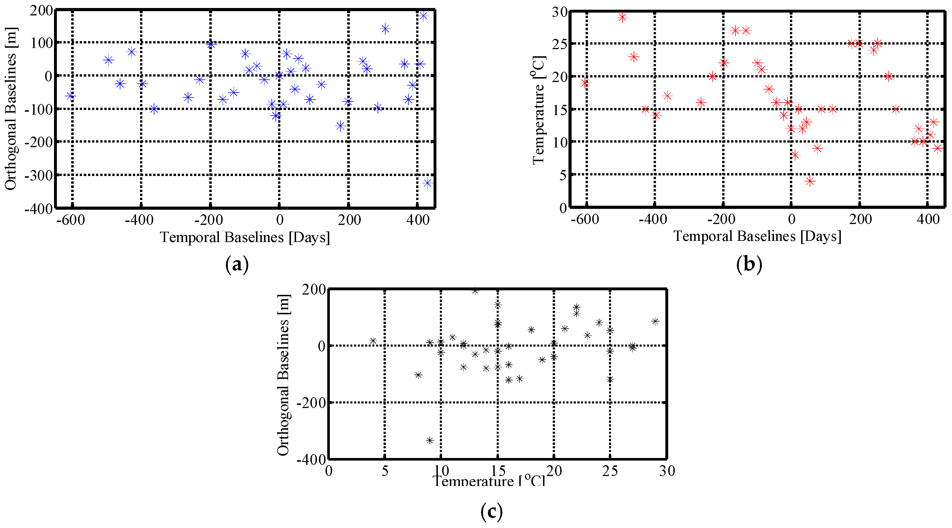
We consider 38 TerraSAR-X images whose spatial and temporal baselines and temperatures are reported in Figure 1, where the distributions of the spatial baselines (orthogonal component) vs. the temporal baselines (Figure 1a), of the temperatures vs. the temporal baselines (Figure 1b), and of the spatial baselines (orthogonal component) vs. the temperatures (Figure 1c) are shown. An average value of the air temperature for each image is used. The total spatial baseline span is about 507 m, thus the Rayleigh resolution in elevation is 18.7 m, the total temporal span is 2.8 years, and the temperature range is around 25 °C. In Figure 1, it can be seen that the two conditions specified in [7,29]—that the observed period has to be as large as possible, and that it is important to minimize the correlation between spatial baselines (orthogonal components), temporal baselines and temperature values—are satisfied.
In processing simulated and real data, we limit the search to two targets (Kmax = 2) per resolution cell, since, in urban applications, the number of scatterers is usually assumed to be one or two, as in all the reported references. In [34], the detection performance of Fast-Sup-GLRT in the 3D case has been extensively analyzed. It was shown that, if the product of the number of acquisitions for the SNR (Signal to Noise Ratio) is sufficiently high, two scatterers can be detected as distinct scatterers, and correctly located, with a probability of detection very close to one and a probability of false alarm very close to zero, even if their spacing is lower than the Rayleigh system resolution.
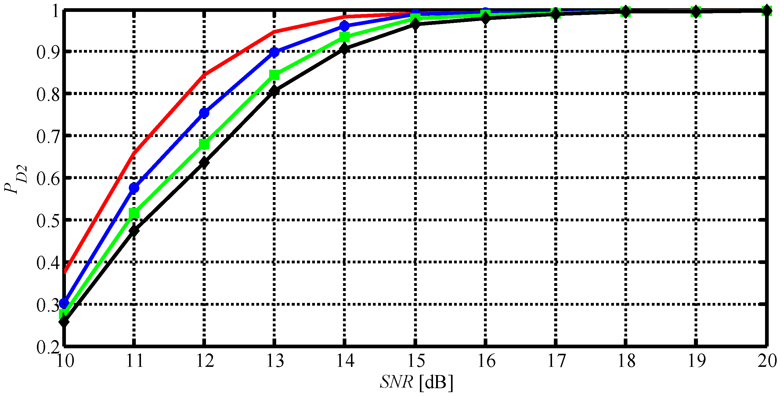
Since, in this paper, we want to show the effectiveness of the proposed method in 5D real case applications, we analyze the impact of data non-idealities (e.g., residual phases) on threshold setting. We simulate a random phase error on each acquisition, so as to induce a temporal decorrelation on the scatterers signals, revealed by different values of the average coherence between the scatterers’ signals at the master and the other acquisitions. We show in Figure 2 the probabilities of detection PD2 for two scatterers at distance Ds = ρs/ηs = 3.1 m, with ηs = 6, obtained from data with no decorrelation (red), and with an average coherence equal to 0.93 (blue), 0.85 (green), and 0.8 (black). We assume a fixed PFA = PFD2 = 10−3, a number of acquisitions M = 38, and we vary the amplitude of the two scatterers such that SNR goes from 10 dB to 20 dB for each scatterer. The detection probabilities have been obtained using the thresholds evaluated using Model (6), where the scatterers are considered fully coherent. The performance loss is negligible for SNR greater than 14 dB. This behavior shows that, for sufficiently high SNR values, a scatterer’s coherence loss, which is adding up to that introduced by additive noise, negligibly impacts the detection performance obtained using the threshold setting based on simulated data. We note that it has been assumed that the scatterers have the same amplitude. In the general case, instead, the scatterers will have different intensities. In this more realistic case, the expected detection performance will be certainly better than the one obtained in the case of equal intensity scatterers with SNR = MinSNR, where MinSNR is the SNR of the weaker scatterer. Then, for finding a lower bound for the detection performance, the probability of detection obtained by considering two scatterers with the same intensity value corresponding to SNR = MinSNR can be considered.
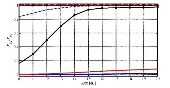
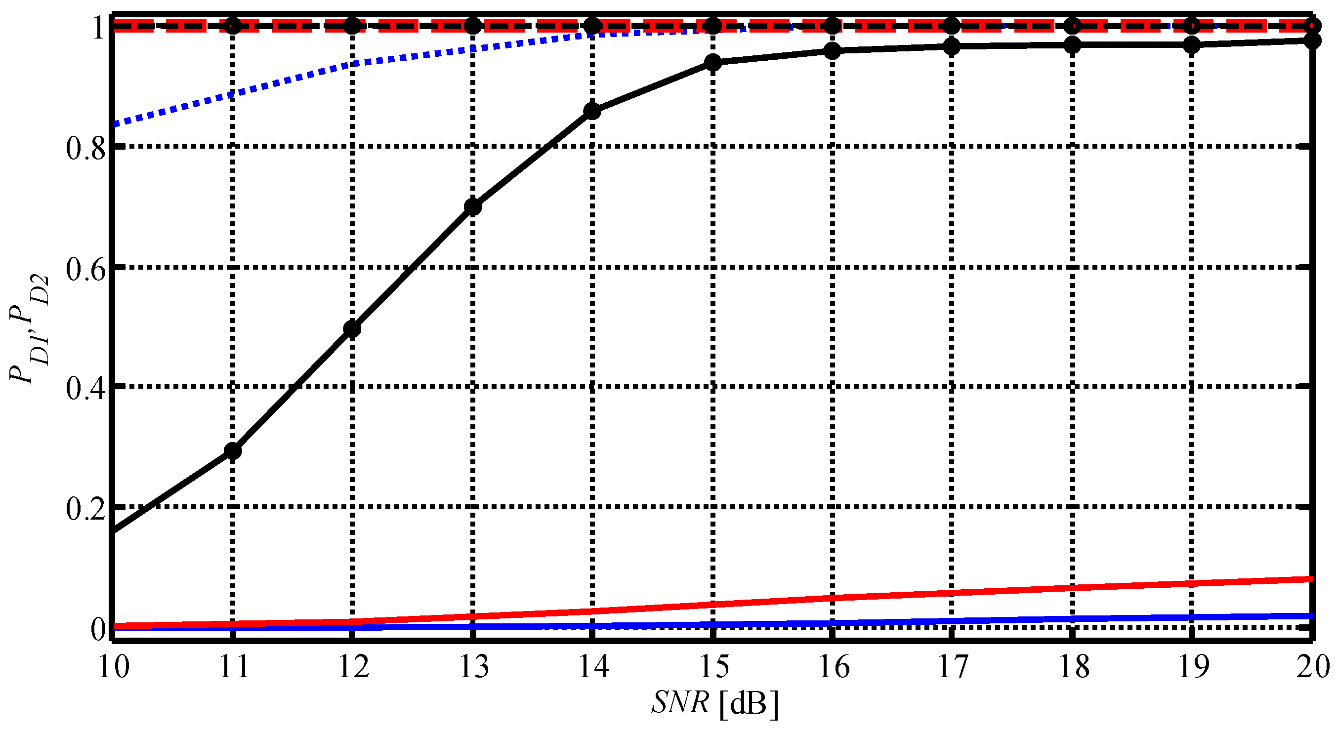
To show the effectiveness of the use of the extended phase Model (4) when temporal deformations are present, we show the detection performance for the case of two scatterers at distance Ds = ρs/ηs = 3.1 m, with ηs = 6, and exhibiting thermal dilation, in particular, for two values of thermal coefficient k = 0.3 mm/°C and k = 0.4 mm/°C. In Figure 3, we report the performance in terms of probabilities of detection PD1 and PD2 for the two cases, when no surface deformation and thermal dilation are considered (3D detector) and when they are taken into account (5D detector). We observe that the 3D detector for data simulated with a thermal coefficient k = 0.3 mm/°C exhibits a PD1 (red, dashed) equal to one, while, for k = 0.4 mm/°C (blue, dashed), the PD1 starts decreasing. The PD2 for the 3D detector in the two cases (red, blue, solid) is very small. It has been considered also the case of k = 0.5 mm/°C, but it has been found that the 3D detector is not able to detect any point (neither single nor double), so that the corresponding detection probabilities are equal to zero. Instead, the 5D detector, as expected, has the same behavior for all the three values of k. The PD1 (black, dashed) is always equal to one, while the PD2 (black, solid) increases with SNR and for an SNR greater than 14 dB is over 0.8. We conclude that the 3D detector, in the presence of thermal dilation deformation, is still able to find single and few double scatterers, when the phenomenon is limited, as in the case of low buildings, since thermal dilation increases linearly with the height. When thermal dilation increases, the 3D detector is not able to find any scatterer. Introducing an extended phase model, as in the 5D detector, allows for detecting with probability one all the singles and with high probability the doubles, provided that the SNR is high enough.
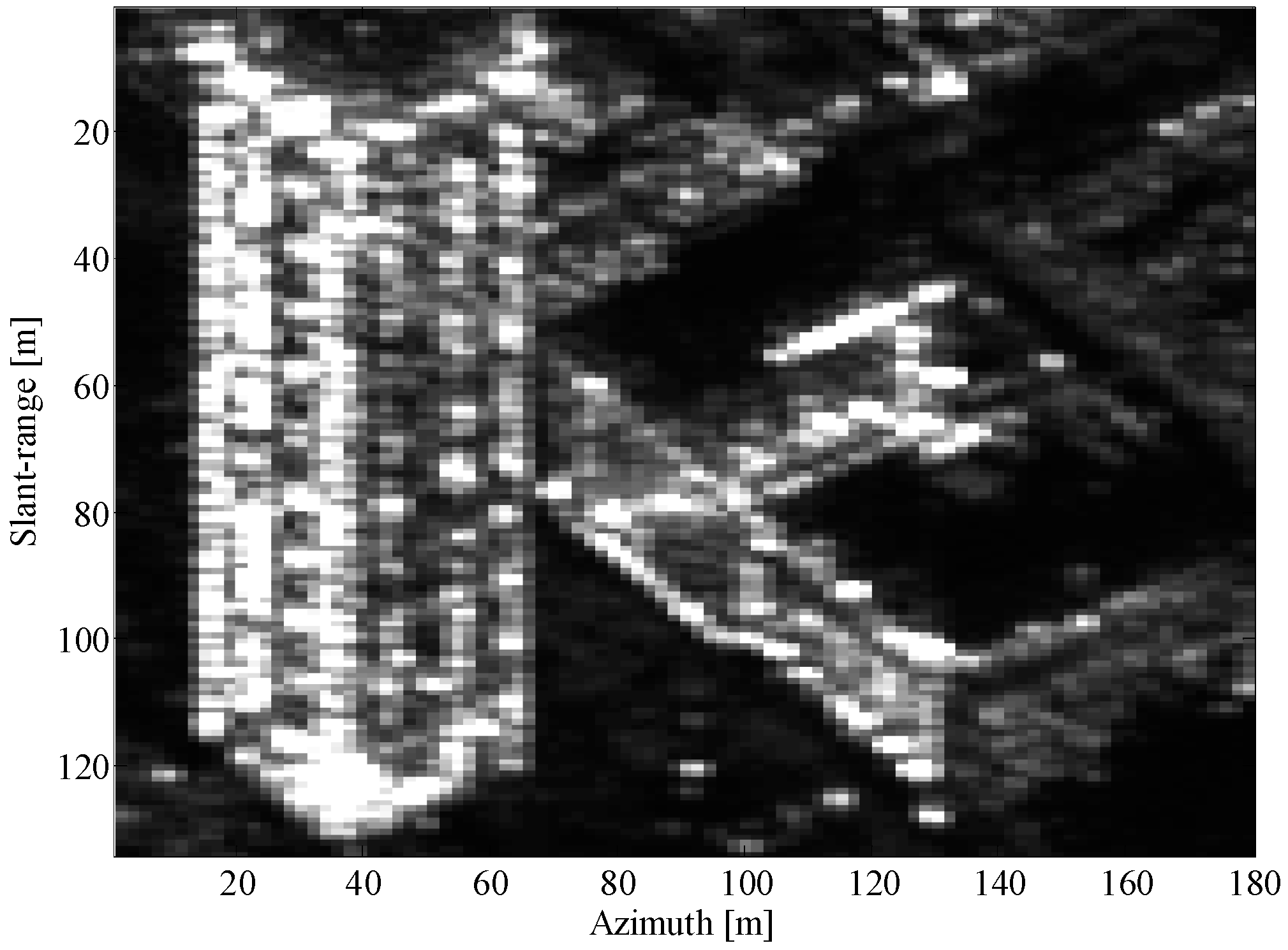
The proposed detector is also tested on the urban area of Barcelona, Spain, where the Art Hotel Tower, 44-storey, 154 m tall, is located (see Figure 4). A very tall building has been chosen, since the detection of scatterers located in a large elevations range is more critical. It is a tower of green colored glass, surrounded by a perimeter structure’s completely white steel exterior at the front and visible, without any coating, so we expect a high sensitivity to temperature changes, as also it has been shown in [8] on the same test site. There is also another building near the tower about 40 m tall, and concrete made, thus it should be less sensitive to temperature changes. We assume a stack of M = 38 range-azimuth focused TerraSAR-X images, whose baselines are shown in Figure 1. The slant range resolution is 1.2 m, the resolution in azimuth is 3.3 m, and the resolution in elevation achieved with the oversampling factor ηs = 6 is 3.1 m (in height 1.8 m) comparable with the resolution in azimuth and range. The thresholds have been computed by Monte Carlo simulation for the considered system parameters (Table 1), fixing PFD2 = PFA = 10−3 and the oversampling factor ηs = 6.
In order to assess the performance of the proposed method with respect to other methods presented in the literature, a fair comparison consists in comparing Fast-Sup-GLRT with another CFAR approach. We consider the Sequential GLRT with Cancellation (SGLRTC) [28], which exhibits a computational complexity equivalent to Fast-Sup-GLRT. As already showed in [34] for the 3D case, SGLRTC is not able to super resolve, i.e., to separate scatterers closer than the system resolution. We do not compare the method with a PS approach because it is not based on a CFAR criterion and is not able to separate double scatterers. Then, it is very difficult to choose a proper metric for performing a fair quantitative comparison between PS and GLRT based aproaches. Anyway, a detailed analysis of the results obtained using SGLRTC and PS approaches has been presented in [23]. It was found that a significant part of the layover-affected pixels along the facades of high-rise buildings have been either totally rejected in the PS processing, or partially rejected, in the sense that a second coherent scatterer is present but has not been individually identified as a PS. This can cause a decrease in the number of points globally detected by the PS technique compared to the one obtained using SGLRTC with the same localization accuracy. Moreover, if double scatterers are erroneously detected as single scatterers, wrong estimates of the scatterer height, temporal deformation and thermal dilation will be provided. This point will be discussed more in details in the following.
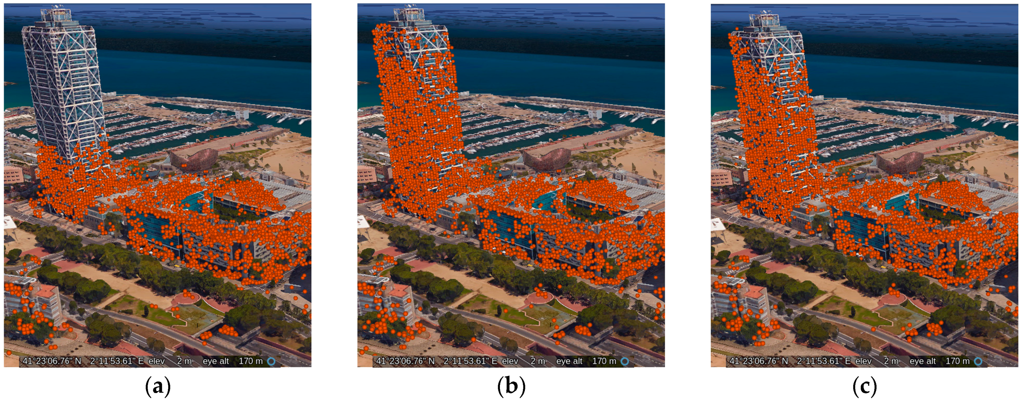
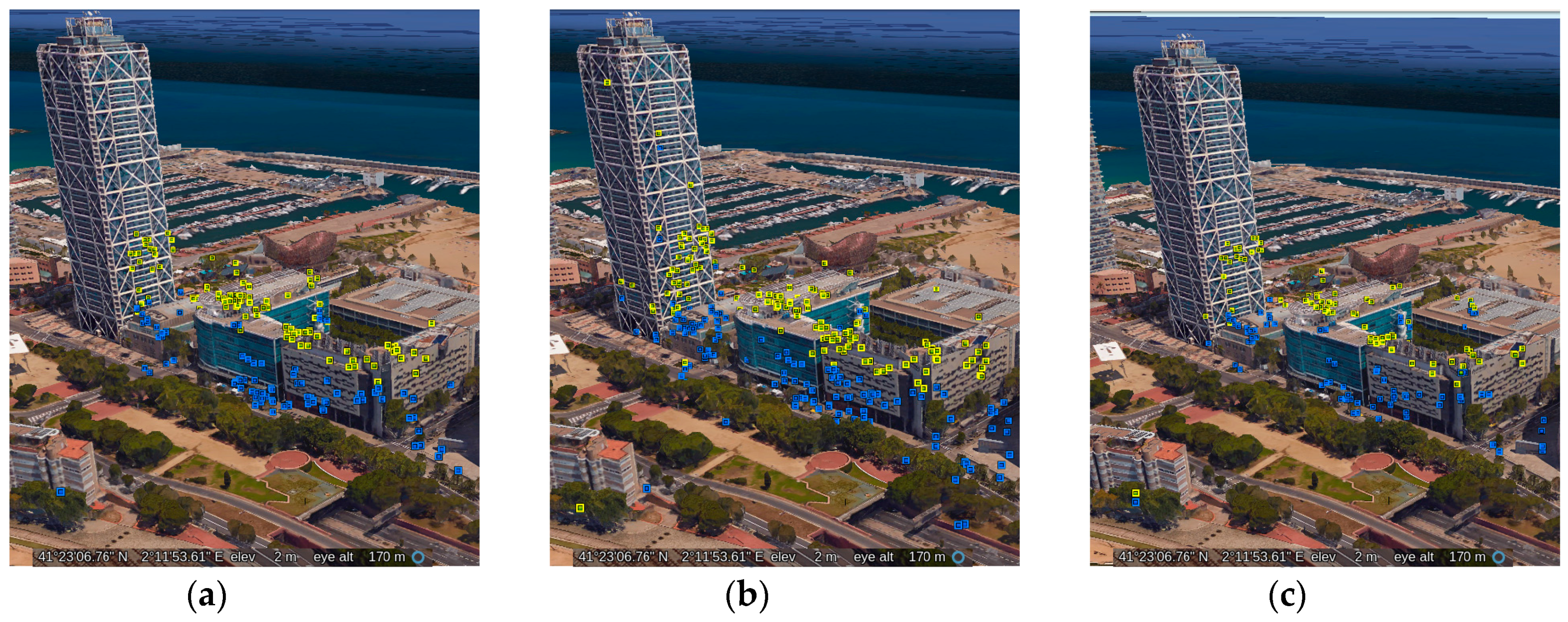
In Figure 4, the SAR intensity image of test site is presented. We compare results obtained in three cases: when no surface deformation and thermal dilation are considered (3D Fast-Sup-GLRT) and when they are taken into account using Fast-Sup-GLRT (5D Fast-Sup-GLRT) and SGLRTC (5D SGLRTC). We note that the grid used for the discretization (6) is such that the M × N measurement matrix Φ in the 3D case is 38 × 95 while in the 5D case is 38 × 13775. In Figure 5, we present the single scatterers detected (red circle single scatterer) and reported on the 3D Google Earth optical image, using 3D Fast-Sup-GLRT (a), 5D Fast-Sup-GLRT (b) and 5D SGLRTC (c). In Figure 6, we present the doubles scatterers detected (lower scatterers in blue, higher scatterers in yellow) and reported on the 3D Google Earth optical image, using 3D Fast-Sup-GLRT (a), 5D Fast-Sup-GLRT (b) and 5D SGLRTC (c). Using 3D Fast-Sup-GLRT, 3729 singles and 208 doubles were found, while using 5D Fast-Sup-GLRT 5206 singles and 292 doubles were detected. The 5D SGLRTC detector, instead, provides 4796 singles and 177 doubles. Then, 5D Fast-Sup-GLRT detector allowed a gain of 40% in additional scatterers (both singles and doubles) with respect to the 3D one ((Points detected 5D − Points detected 3D)/(Points detected 3D) × 100), while it allowed an improvement of 10% in the number of detected scatterers with respect to 5D SGLRTC.
We note that the number of detected double scatterers is not very high, thus indicating that not many coherent double scatterers are present in the observed scene. This certainly depends on the site geometry and on the range and azimuth resolutions of the StripMap TSX images, which are not very high. Anyway, we note that the detected scatterers appear correctly located on the buildings and on the ground, thus confirming their reliability, and that the number of doubles detected by 5D SGLRTC is even lower than the one obtained using 5D Fast-Sup-GLRT. Moreover, the density of the detected doubles is in accordance with the one shown on the same site in [23], although, in [23], a larger number of baselines was used.
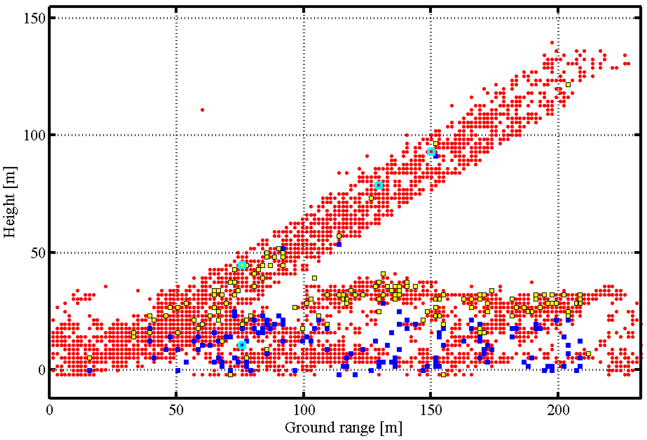
For highlighting the layover effect and the double scatterers localization, the scatterers detected with 5D Fast-Sup-GLRT have been projected onto the ground range-height plane and plotted in Figure 7 (single scatterers in red, lower double scatterers in blue, higher double scatterers in yellow). The ground plane, the layover areas and the roofs appear clearly distinguishable. Moreover, it appears that the higher double scatterers are prevalently located in the layover area on the skyscraper façade and on the lower building roof, while the lower double scatterers are prevalently located on the ground structures. In Figure 8 the detected scatterers are positioned on 3D Google Earth optical image. Height values have been used for colorization of the points (single circle, double square): using 3D Fast-Sup-GLRT (a); 5D Fast-Sup-GLRT (b); and 5D SGLRTC (c).
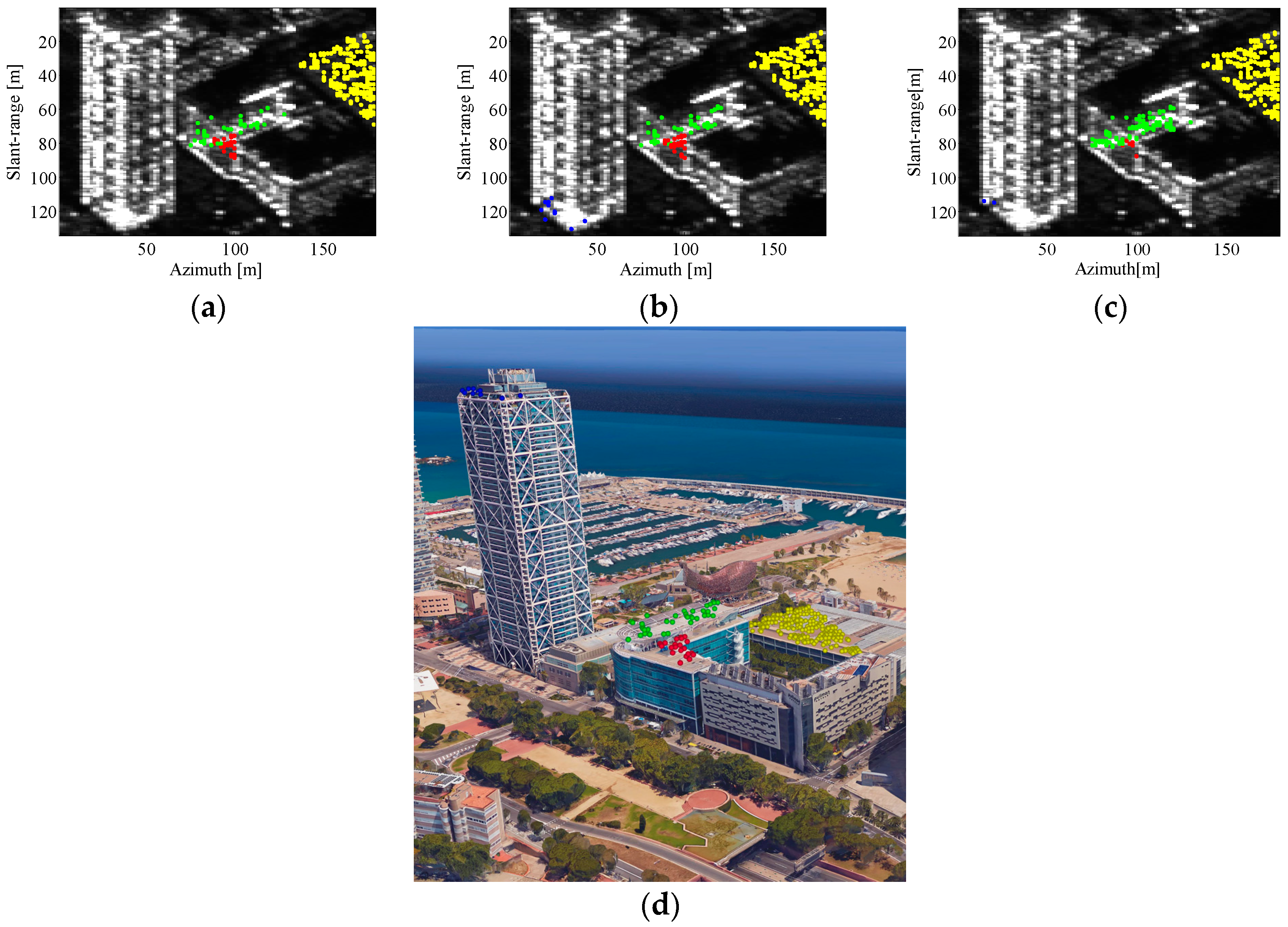
In order to assess the height estimation performance of the presented approach, we selected four groups of points identifiable on the roof of two buildings whose true height can be recovered and it is used as ground truth. In Figure 9, we show the points detected using 3D Fast-Sup-GLRT (a), 5D Fast-Sup-GLRT (b) and 5D SGLRTC (c) on the SAR intensity image and on the 3D Google Earth optical image for the 5D Fast-Sup-GLRT detector (d). In Table 2, we report the true heights, the average and the Root Mean Square Error (RMSE) values of the estimated heights for the four groups of points.
We note that, for the blue points, which are on the top of the tower, we can only consider the 5D case, as in the 3D case the top of the tower is not reached. For all of the four groups, the RMSE values are of the order of the height resolution, which is 1.8 m. We do not find substantial differences, between 3D Fast-Sup-GLRT, 5D Fast-Sup-GLRT and 5D SGLRTC, for the error values of the scatterers located on the low building, since, in this case, the effect of the thermal dilation is negligible and the three algorithms behave in the same way. Instead, the scatteres located on the top of the tower, which exhibit a more significant thermal dilation, are not selected by the 3D detector. Then, we can conclude that the estimates provided by the detected points are accurate enough in the three cases, proving that the adopted detection criterion, consisting of keeping constant and low the probability of false alarm, allows for selecting only reliable scatterers, providing estimates with comparable accuracy.
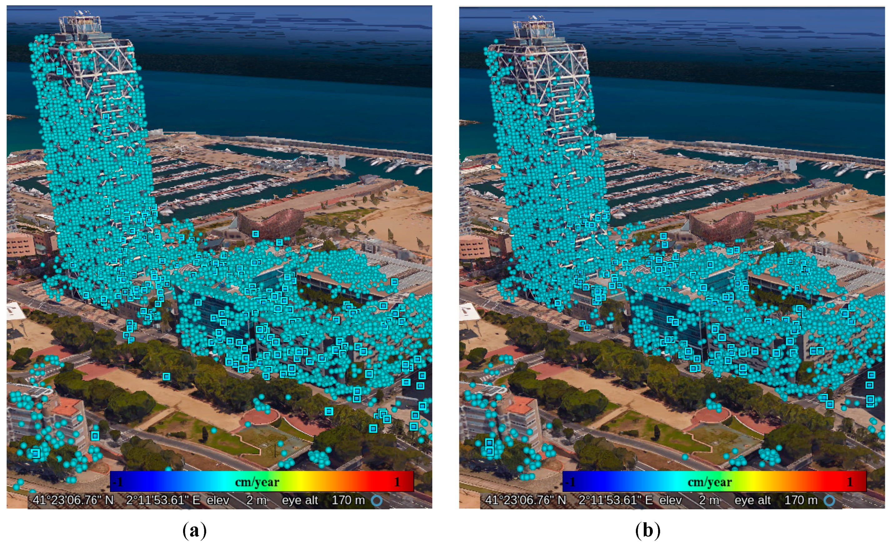
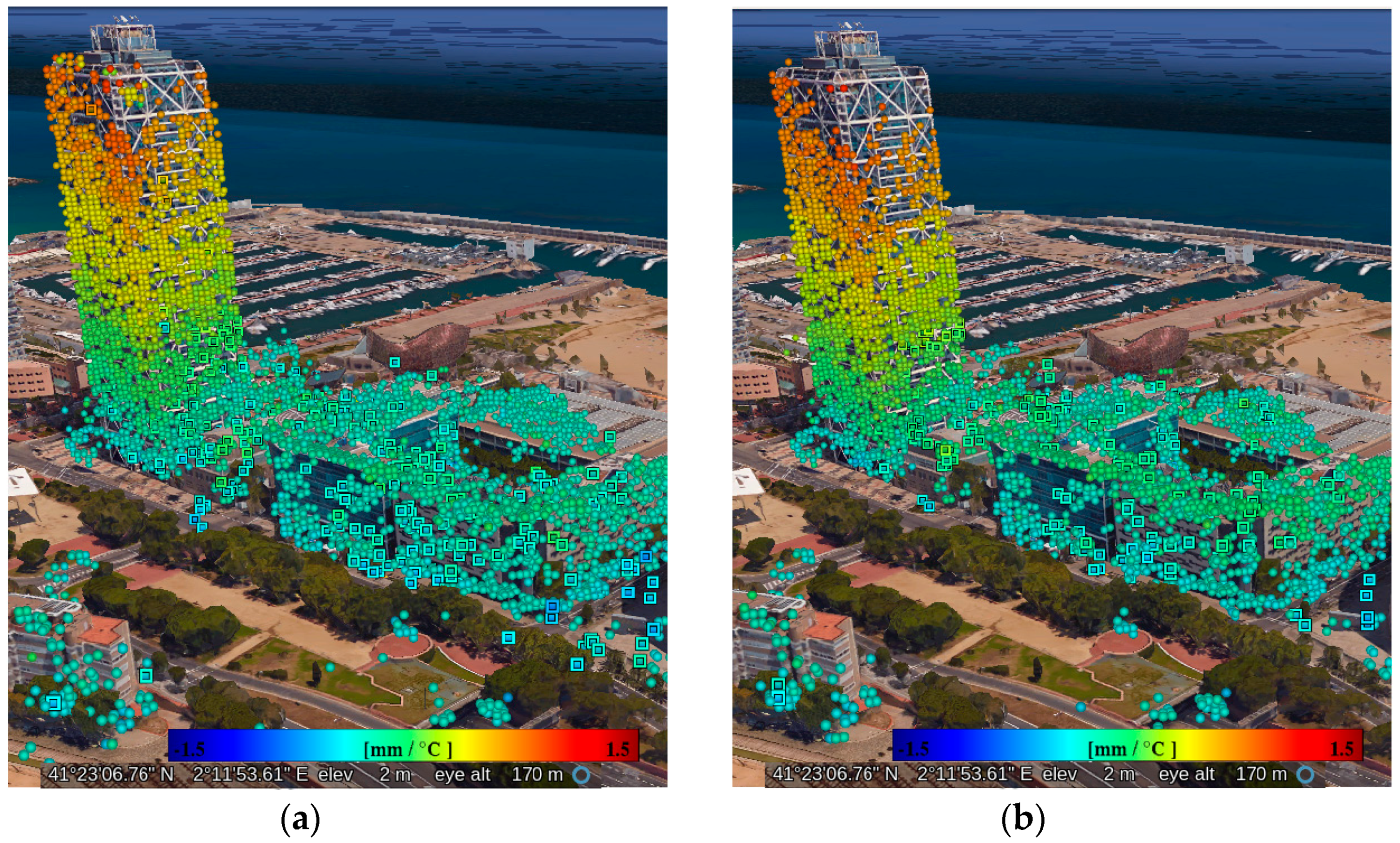
In Figure 10 and Figure 11, we report the estimated average deformation velocity map, with velocity expressed in cm/year, and the estimated thermal dilation map, with dilation coefficient expressed in mm/°C, obtained using 5D Fast-Sup-GLRT (a) and 5D SGLRTC (b).
We note that there is no deformation velocity while the contribution of thermal dilation is considerable for the taller building. In fact, the main structure of the Art Hotel Tower is external and completely in steel, hence directly exposed to the seasonal temperature changes. The thermal map shows values that roughly range from 0 to 1.5 mm/°C, compatible with a coefficient of thermal expansion of 12 × 10−6/°C for a steel structure of 154 m. For the other building concrete made, the values of the thermal map roughly range from 0 to 0.3 mm/°C, and are compatible with a coefficient of thermal expansion of 9.8 × 10⁻⁶/°C for a concrete structure of 41 m. There are not significant differences between the two methods. We cannot provide a ground truth validation of the obtained results, but, in [8], an experiment is presented on the same test site where the thermal dilation coefficients on the Art Hotel Tower, estimated from 28 StripMap TSX images and using an extended PSI model, were compared with those derived by Ku-band Ground Based SAR (GBSAR) data, finding a good agreement. The range values of the thermal dilation map estimated by Fast-Sup-GLRT is in accordance with the values estimated in [8].
The added value of the presented approach with respect to the one in [8] is to resolve a layover looking for multiple scatterers and to control the false alarm rate in order to mitigate the effect of all the sources of noise and artifacts, such as water vapor, humidity, mechanical noise, and wind.
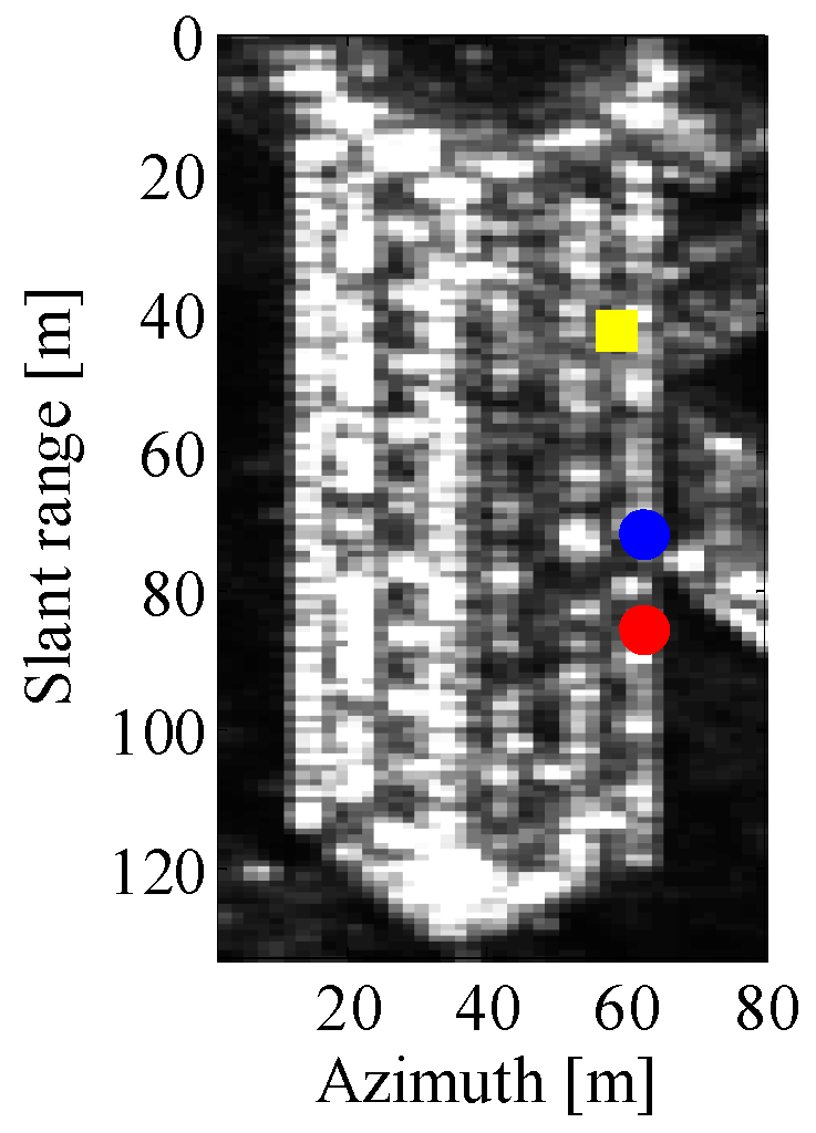
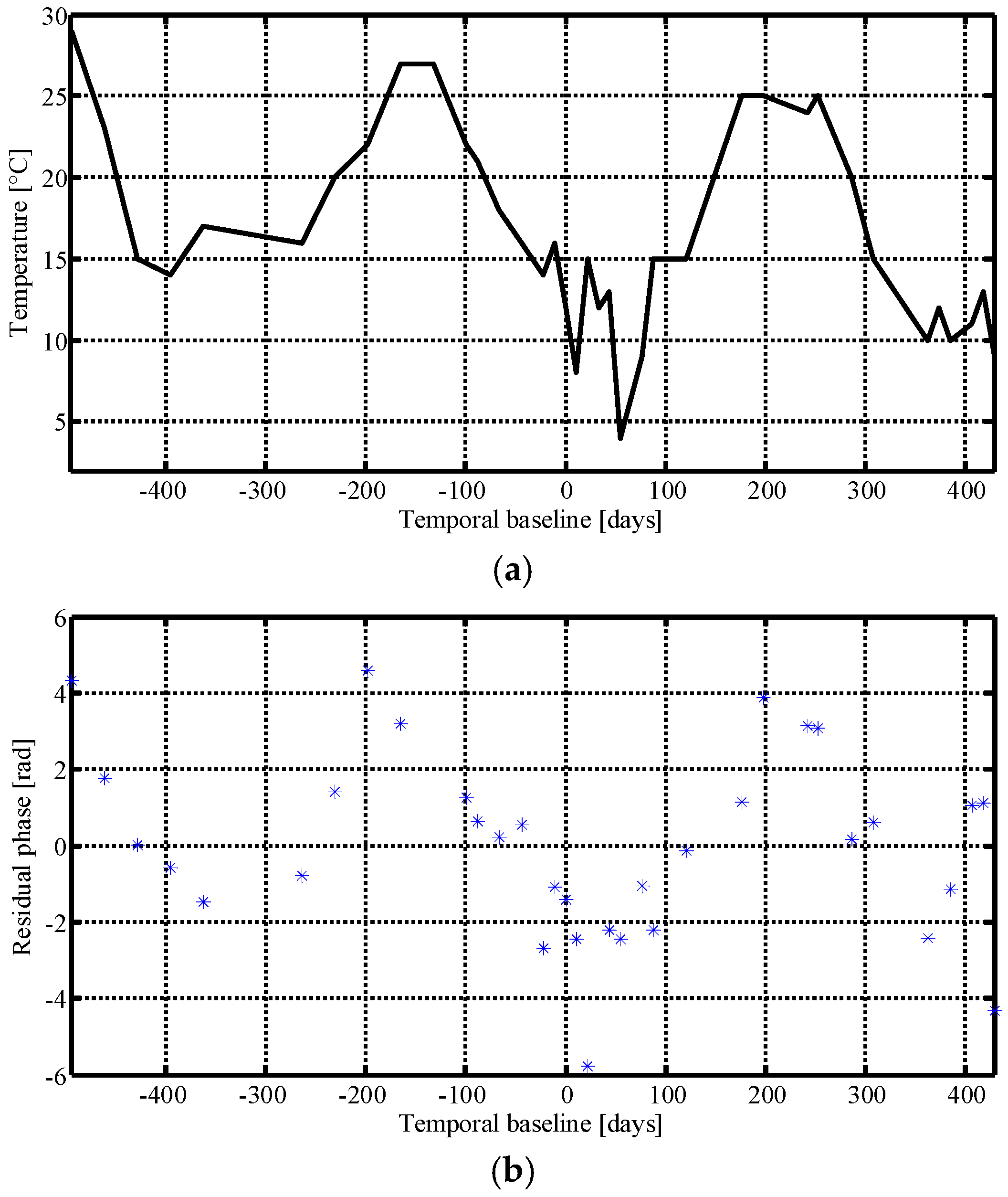
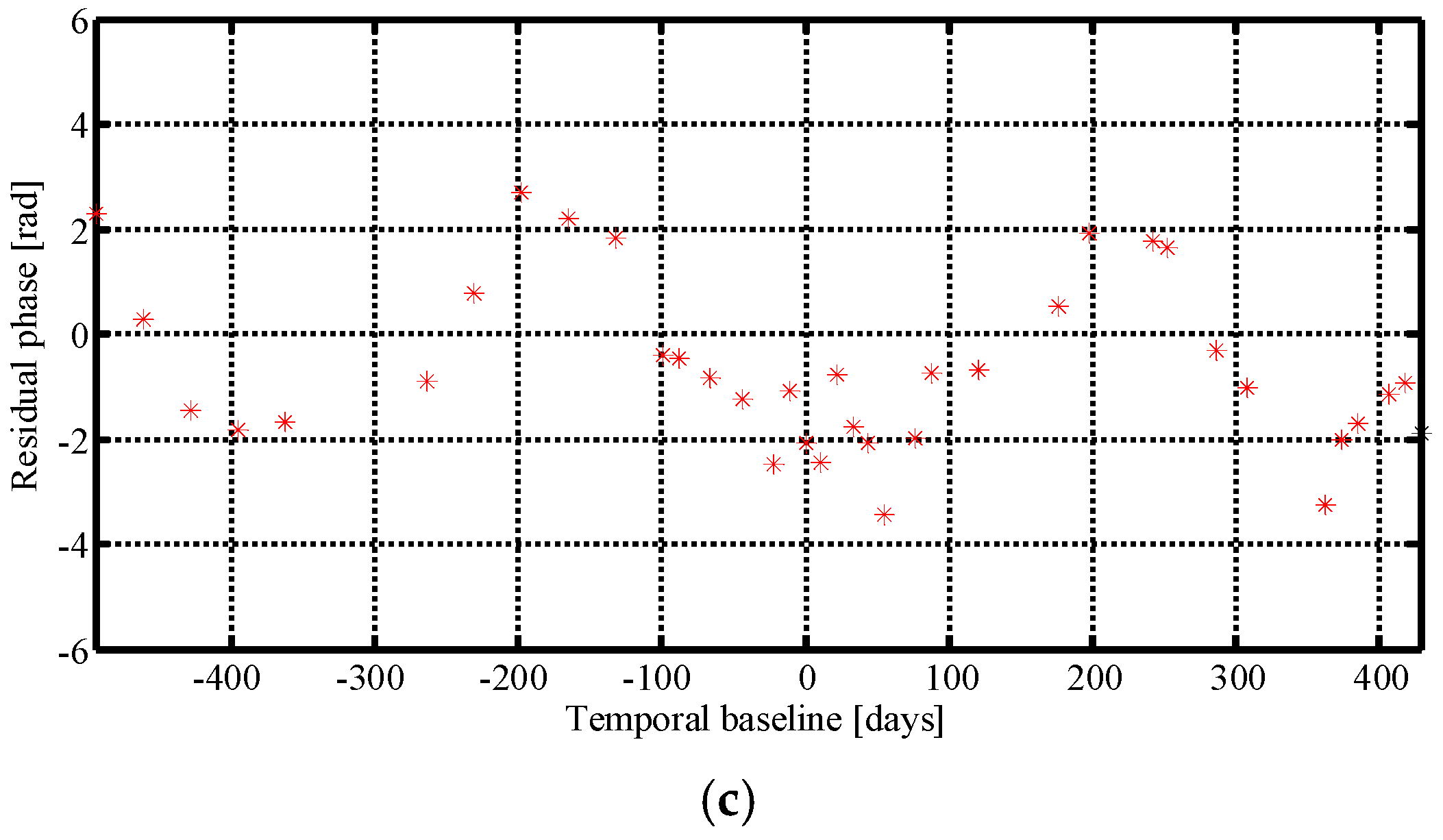
For a further verification of the obtained results, we considered two single scatterers (blue and red circle) detected with 5D Fast-Sup-GLRT on the tower at the heights 78 m and 83 m, and shown in Figure 12. The height localization of the two scatterers is highlighted in Figure 7 with red circles with a cyan contour. In Figure 13, we plot the behavior of the residual interferometric phases, obtained after compensation of the topographic phase term related to the scatterers height, against temporal baselines and temperatures. In Figure 13a, we show the temporal changes of the temperature values and, in Figure 13b,c, the residual phases of the two scatterers vs. the temporal baselines. It is quite evident that that the residual phases exhibit the same temporal behavior of the temperatures, thus confirming that residual phases can be produced by a thermal dilation effect. Then, in Figure 14a,b, we plot the residual phases vs. the temperature. We notice that the exhibited trend is linear and in good accordance with the linear trend corresponding to the estimated thermal dilation coefficients of the two considered scatterers, thus confirming a strong relation with the thermal dilation effect.
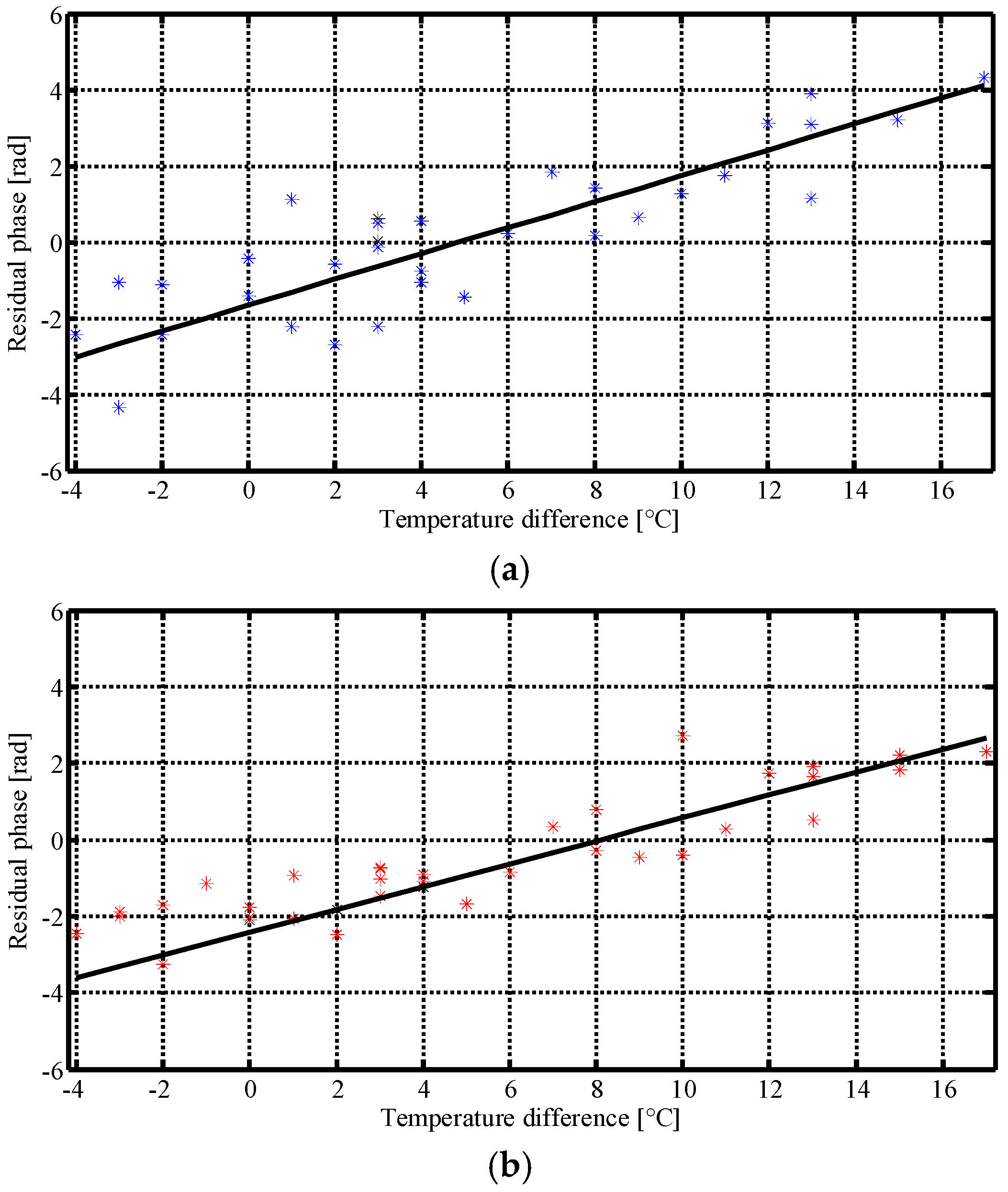
The same analysis has been performed on a couple of double scatterers detected using 5D Fast-Sup-GLRT, and reported with a yellow square on the SAR intensity image in Figure 12. The height localization of the two double scatterers is highlighted in Figure 7 with yellow and blue squares with a cyan contour. It can be seen that the scatterer with a higher height is on the tower, which has an outer steel structure, while the other, that exhibits a lower height, is on a concrete made ground structure. For evaluating the residual phase of these double scatterers, the first step was the computation of the data components associated with each of the two scatterers, performed by subtracting the estimated scatterers’ contribution from the overall data signal. Then, the residual phases, obtained after the topographic term compensation of both data components, have been evaluated and plotted vs. the temperatures in Figure 15a,b for the higher (yellow square) and the lower scatterer (yellow circle), respectively. The corresponding estimated heights and thermal dilation coefficients are of about 45 m and 0.4 mm/°C for the higher scatterer, and 10 m and 0 mm/°C for the lower scatterer. The related linear phases are also plotted in Figure 15a,b. It can be noted that the estimated values are revealing a thermal dilation effect on the tower, due to the outer steel structure, and an absence of thermal effect on the concrete made ground structure, as expected. Moreover, we notice that the residual phases of both scatterers’ components are in a good accordance with the estimated phases.
For showing the importance of separating double targets, when present, we considered the results obtained by setting Kmax = 1, which amounts to searching only single scatterers. In this case, 115 of the 292 double scatterers are still detected as single scatterers, while the others are lost. Anyway, the estimate of their height and/or deformation velocity and thermal dilation coefficient can be different from the one provided by the search of double scatterers. For instance, the double scatterer considered previously, shown with a yellow square in Figure 12, is still detected as a single scatterer with an estimated height of about 42 m and a thermal dilation coefficient of 0.3 mm/°C. To verify if this estimate is satisfying, we report the residual phase of the considered pixel of the image stack, after topographic term compensation, in Figure 15c. It is quite evident that the accordance between the residual phase values and the estimated linear phase is weaker than the one found in the double scatterer case. This example shows that the separation of double scatterers is important for obtaining more accurate estimates of height, deformation velocity and thermal dilation coefficient in urban structures’ monitoring.
4. Conclusions
In this paper, a fast statistical test for detecting at most Kmax scatterers from multi-baseline SAR images has been extended to 5D tomographic reconstruction.
The test does not require the knowledge of the noise variance and can be evaluated in terms of probability of detection and probability of false alarms. Then, fixing a proper threshold on the base of an assigned PFA, the proposed method is able to limit the outliers and misdetections, and provides reliable estimates of the position and of the temporal and thermal deformations of the detected scatterers (5D tomography). The practical application of the method to the 5D case is made possible by the fact that the computational cost is linear with the size N of the reflectivity unknown vector. This allows for considering an extended phase model taking into account time deformation and/or dilation (4D and 5D). Performance analysis is carried out on StripMap TSX data of an area of Barcelona (Spain) where, due to the high resolution, the layover effect is present. Presented results show the effectiveness of the proposed approach in detecting reliable single and double scatterers in urban areas, useful for the measurement of surface deformations of manmade structures. Moreover, it has been shown that taking into account velocity deformation and thermal dilation helps in recovering more scatterers, both single and double, and also in detecting the top of tall buildings. The two contributions, linear temporal deformation and thermal dilation, have been separated and estimated. A physical interpretation of the detected thermal dilation phenomenon, in accordance with the geometry and material of the structure considered, has been given. In addition, it has been shown that the separation of double scatterers allows for detecting a larger number of reliable scatterers and for obtaining more accurate estimates’ height, deformation velocity and thermal dilation coefficient in urban structures monitoring.
Acknowledgments
We thank the DLR, for providing the TSX data (proposal MTH3182). We thank the European Space Agency (ESA), for providing the software NEST (Next ESA SAR Toolbox).
Author Contributions
Alessandra Budillon and Gilda Schirinzi developed the algorithm; Angel Caroline Johnsy pre-processed real data and produced the geocoded results; all of the authors contributed and performed the experiments; and all of the authors contributed to the paper writing.
Conflicts of Interest
The authors declare no conflict of interest.
References
- Baselice, F.; Ferraioli, G.; Pascazio, V.; Schirinzi, G. Contextual information-based multichannel synthetic aperture radar interferometry: Addressing DEM reconstruction using contextual information. IEEE Signal Proc. Mag. 2014, 31, 59–68. [Google Scholar] [CrossRef]
- Fornaro, G.; Lombardini, F.; Pauciullo, A.; Reale, D.; Viviani, F. Tomographic Processing of Interferometric SAR Data: Developments, applications, and future research perspectives. IEEE Signal Process. Mag. 2014, 31, 41–50. [Google Scholar] [CrossRef]
- Baselice, F.; Budillon, A.; Ferraioli, G.; Pascazio, V.; Schirinzi, G. Multibaseline SAR Interferometry from Complex Data. IEEE J. Sel. Top. Appl. Earth Obs. Remote Sens. 2014, 7, 2911–2918. [Google Scholar] [CrossRef]
- Gabriel, A.K.; Goldstein, R.M.; Zebker, H.A. Mapping small elevation changes over large areas: Differential radar interferometry. J. Geophys. Res. 1989, 94, 9183–9191. [Google Scholar] [CrossRef]
- Ferretti, A.; Prati, C.; Rocca, F. Nonlinear subsidence rate estimation using permanent scatterers in differential SAR interferometry. IEEE Trans. Geosci. Remote Sens. 2000, 38, 2202–2212. [Google Scholar] [CrossRef]
- Gernhardt, S.; Adam, N.; Eineder, M.; Bamler, R. Potential of very high resolution SAR for persistent scatterer interferometry in urban areas. Ann. GIS 2010, 16, 103–111. [Google Scholar] [CrossRef]
- Crosetto, M.; Monserrat, O.; Iglesias, R.; Crippa, B. Persistent scatterer interferometry: Potential, limits and initial C- and X-band comparison. Photogramm. Eng. Remote Sens. 2010, 76, 1061–1069. [Google Scholar] [CrossRef]
- Crosetto, M.; Monserrat, O.; Cuevas-González, M.; Devanthéry, N.; Luzi, G.; Crippa, B. Measuring thermal expansion using X-band persistent scatterer interferometry. ISPRS J. Photogramm. Remote Sens. 2015, 100, 84–91. [Google Scholar] [CrossRef]
- Monserrat, O.; Crosetto, M.; Cuevas, M.; Crippa, B. The thermal expansion component of Persistent Scatterer Interferometry observations. IEEE Geosci. Remote Sens. Lett. 2011, 8, 864–868. [Google Scholar] [CrossRef]
- Devanthéry, N.; Crosetto, M.; Monserrat, O.; Cuevas-González, M.; Crippa, B. An Approach to Persistent Scatterer Interferometry. Remote Sens. 2014, 6, 6662–6679. [Google Scholar] [CrossRef]
- Ferretti, A.; Fumagalli, A.; Novali, F.; Prati, C.; Rocca, F.; Rucci, A. A new algorithm for processing interferometric data-stacks: SqueeSAR. IEEE Trans. Geosci. Remote Sens. 2011, 49, 3460–3470. [Google Scholar] [CrossRef]
- Perissin, D.; Wang, T. Repeat-pass SAR interferometry with partially coherent targets. IEEE Trans. Geosci. Remote Sens. 2012, 50, 271–280. [Google Scholar] [CrossRef]
- Ferretti, A.; Bianchi, M.; Prati, C.; Rocca, F. Higher-order permanent scatterers analysis. EURASIP J. Appl. Signal Proc. 2005, 2005, 3231–3242. [Google Scholar] [CrossRef]
- Reigber, A.; Moreira, A. First Demonstration of Airborne SAR Tomography Using Multibaseline L-band Data. IEEE Trans. Geosci. Remote Sens. 2000, 38, 2142–2152. [Google Scholar] [CrossRef]
- Lombardini, F. Differential tomography: A new framework for SAR interferometry. IEEE Trans. Geosci. Remote Sens. 2005, 43, 37–44. [Google Scholar] [CrossRef]
- Fornaro, G.; Lombardini, F.; Serafino, F. Three-Dimensional Multipass SAR Focusing: Experiments with Long-Term Spaceborne Data. IEEE Trans. Geosci. Remote Sens. 2005, 40, 702–714. [Google Scholar] [CrossRef]
- Budillon, A.; Evangelista, A.; Schirinzi, G. Three-Dimensional SAR Focusing From Multipass Signals Using Compressive Sampling. IEEE Trans. Geosci. Remote Sens. 2011, 49, 488–499. [Google Scholar] [CrossRef]
- Zhu, X.X.; Bamler, R. Tomographic SAR Inversion by L1-Norm Regularization—The Compressive Sensing Approach. IEEE Trans. Geosci. Remote Sens. 2010, 48, 3839–3846. [Google Scholar] [CrossRef]
- Zhu, X.X.; Bamler, R. Super-Resolution Power and Robustness of Compressive Sensing for Spectral Estimation with Application to Spaceborne Tomographic SAR. IEEE Trans. Geosci. Remote Sens. 2012, 50, 247–258. [Google Scholar] [CrossRef]
- Budillon, A.; Ferraioli, G.; Schirinzi, G. Localization Performance of Multiple Scatterers in Compressive Sampling SAR Tomography: Results on COSMO-SkyMed Data. IEEE J. Sel. Top. Appl. Earth Obs. Remote Sens. 2014, 7, 2902–2910. [Google Scholar] [CrossRef]
- Zhu, X.X.; Shahzad, M. Façade Reconstruction Using Multiview Spaceborne TomoSAR Point Clouds. IEEE Trans. Geosci. Remote Sens. 2014, 52, 3541–3552. [Google Scholar] [CrossRef]
- D’Hondt, O.; Guillaso, S.; Hellwich, O. Geometric primitive extraction for 3d reconstruction of urban areas from tomographic SAR data. In Proceedings of the Joint Urban Remote Sensing Event (JURSE), Sao Paulo, Brazil, 21–23 April 2013; pp. 206–209. [Google Scholar]
- Siddique, M.A.; Wegmüller, U.; Hajnsek, I.; Frey, O. Single-Look SAR Tomography as an Add-On to PSI for Improved Deformation Analysis in Urban Areas. IEEE Trans. Geosci. Remote Sens. 2016, 54, 6119–6137. [Google Scholar] [CrossRef]
- Ma, P.; Lin, H. Robust Detection of Single and Double Persistent Scatterers in Urban Built Environments. IEEE Trans. Geosci. Remote Sens. 2016, 54, 2124–2139. [Google Scholar] [CrossRef]
- Kelly, E.J. An adaptive detection algorithm. IEEE Trans. Aerosp. Electron. Syst. 1986, 2, 115–127. [Google Scholar] [CrossRef]
- Ciuonzo, D.; De Maio, A.; Orlando, D. A unifying framework for adaptive radar detection in homogeneous plus structured interference—Part I: On the maximal invariant statistic. IEEE Trans. Signal Proc. 2016, 64, 2894–2906. [Google Scholar] [CrossRef]
- Ciuonzo, D.; De Maio, A.; Orlando, D. A unifying framework for adaptive radar detection in homogeneous plus structured interference—Part II: Detectors design. IEEE Trans. Signal Proc. 2016, 64, 2907–2919. [Google Scholar] [CrossRef]
- Pauciullo, A.; Reale, D.; De Maio, A.; Fornaro, G. Detection of Double Scatterers in SAR Tomography. IEEE Trans. Geosci. Remote Sens. 2012, 50, 3567–3586. [Google Scholar] [CrossRef]
- Fornaro, G.; Serafino, F.; Reale, D. 4D SAR imaging for height estimation and monitoring of single and double scatterers. IEEE Trans. Geosci. Remote Sens. 2009, 47, 224–237. [Google Scholar] [CrossRef]
- Fornaro, G.; Reale, D.; Verde, S. Bridge thermal dilation monitoring with millimeter sensitivity via multidimensional SAR imaging. IEEE Geosci. Remote Sens. Lett. 2013, 10, 677–681. [Google Scholar] [CrossRef]
- Reale, D.; Fornaro, G.; Pauciullo, A. Extension of 4D SAR imaging to the monitoring of thermally dilating scatterers. IEEE Trans. Geosci. Remote Sens. 2013, 51, 5296–5306. [Google Scholar] [CrossRef]
- Budillon, A.; Schirinzi, G. GLRT Based on Support Estimation for Multiple Scatterers Detection in SAR Tomography. IEEE J. Sel. Top. Appl. Earth Obs. Remote Sens. 2016, 9, 1086–1094. [Google Scholar] [CrossRef]
- Gini, F.; Lombardini, F.; Montanari, M. Layover solution in multibaseline SAR interferometry. IEEE Trans. Aerosp. Electron. Syst. 2002, 38, 1344–1356. [Google Scholar] [CrossRef]
- Budillon, A.; Johnsy, A.C.; Schirinzi, G. A Fast Support Detector for Super-Resolution Localization of Multiple Scatterers in SAR Tomography. IEEE J. Sel. Top. Appl. Earth Obs. Remote Sens. 2017, 10, 1–12. [Google Scholar] [CrossRef]
- Madsen, S.N.; Zebker, H.A.; Martin, J. Topographic mapping using radar interferometry: Processing techniques. IEEE Trans. Geosci. Remote Sens. 1993, 31, 246–256. [Google Scholar] [CrossRef]
- Budillon, A.; Schirinzi, G. Performance Evaluation of a GLRT Moving Target Detector for TerraSAR-X along-track interferometric data. IEEE Trans. Geosci. Remote Sens. 2015, 53, 3350–3360. [Google Scholar] [CrossRef]
- Stoica, P.; Yngve, S.; Jian, Li. On information criteria and the generalized likelihood ratio test of model order selection. IEEE Signal Proc. Lett. 2004, 11, 794–797. [Google Scholar] [CrossRef]
- Xu, L.; Li, J. Iterative generalized-likelihood ratio test for MIMO radar. IEEE Trans. Signal Proc. 2007, 55, 2375–2385. [Google Scholar] [CrossRef]
- Tropp, J. Greed is good: Algorithmic results for sparse approximation. IEEE Trans. Inf. Theory 2004, 50, 2231–2242. [Google Scholar] [CrossRef]
Figure 1.
(a) distribution of the spatial baselines (orthogonal components) vs. the temporal baselines; (b) distribution of the temperature values vs. the temporal baselines; (c) distribution of the spatial baselines (orthogonal components) vs. temperature values.
Figure 1.
(a) distribution of the spatial baselines (orthogonal components) vs. the temporal baselines; (b) distribution of the temperature values vs. the temporal baselines; (c) distribution of the spatial baselines (orthogonal components) vs. temperature values.

Figure 2.
Probabilities of detection PD2 for Fast-Sup-GLRT, with a fixed PFA = PFD2 = 10−3, M = 38 and different values of SNR, for two scatterers at distance Ds = 3.1 m, for the cases of fully correlated scatterers (solid, red), and partially correlated scatterers with average coherence 0.93 (circle, blue), 0.85 (square, green), 0.8 (diamond, black) using the simulated thresholds obtained for the no decorrelation case.

Figure 3.
Probabilities of detection PD1 and PD2 for Fast-Sup-GLRT, with a fixed PFA = PFD2 = 10−3, M = 38 and different values of SNR, for two scatterers at distance Ds = 3.1 m, and exhibiting thermal dilation. The PD1 (in dashed line) and PD2 (in solid line) for the 3D detector are shown in red for k = 0.3 mm/°C, and in blue for k = 0.4 mm/°C. The PD1 (in dashed line) and PD2 (in solid line) for the 5D detector are shown in black and are the same for both the thermal coefficient values.

Figure 4.
Intensity SAR image of Art Hotel Tower, Barcelona, Spain (Copyright German Aerospace Centre DLR 2007–2010).
Figure 4.
Intensity SAR image of Art Hotel Tower, Barcelona, Spain (Copyright German Aerospace Centre DLR 2007–2010).

Figure 5.
Single scatterers detected and positioned on 3D Google Earth optical image, using 3D Fast-Sup-GLRT (a); 5D Fast-Sup-GLRT (b); and 5D SGLRTC (c).
Figure 5.
Single scatterers detected and positioned on 3D Google Earth optical image, using 3D Fast-Sup-GLRT (a); 5D Fast-Sup-GLRT (b); and 5D SGLRTC (c).

Figure 6.
Double Scatterers (first in blue, second in yellow) detected and positioned Fast-Sup-GLRT on 3D Google Earth optical image, using 3D Fast-Sup-GLRT (a), 5D Fast-Sup-GLRT (b), and 5D SGLRTC (c).
Figure 6.
Double Scatterers (first in blue, second in yellow) detected and positioned Fast-Sup-GLRT on 3D Google Earth optical image, using 3D Fast-Sup-GLRT (a), 5D Fast-Sup-GLRT (b), and 5D SGLRTC (c).

Figure 7.
Single (red) and Double Scatterers (lower scatterer in blue, higher scatterer in yellow) detected using 5D Fast-Sup-GLRT, in the ground range–height plane and the three scatterers used for the phase history in cyan contour.
Figure 7.
Single (red) and Double Scatterers (lower scatterer in blue, higher scatterer in yellow) detected using 5D Fast-Sup-GLRT, in the ground range–height plane and the three scatterers used for the phase history in cyan contour.

Figure 8.
Scatterers detected and positioned on 3D Google Earth optical image. Height values have been used for colorization of the points (single circle, double square): using 3D Fast-Sup-GLRT (a); 5D Fast-Sup-GLRT (b); and 5D SGLRTC (c).
Figure 8.
Scatterers detected and positioned on 3D Google Earth optical image. Height values have been used for colorization of the points (single circle, double square): using 3D Fast-Sup-GLRT (a); 5D Fast-Sup-GLRT (b); and 5D SGLRTC (c).

Figure 9.
Scatterers detected used to asses height estimation errors, are shown on SAR intensity image using 3D Fast-Sup-GLRT (a); 5D Fast-Sup-GLRT (b); and 5D SGLRTC (c); and on the 3D Google Earth optical image for 5D Fast-Sup-GLRT (d).
Figure 9.
Scatterers detected used to asses height estimation errors, are shown on SAR intensity image using 3D Fast-Sup-GLRT (a); 5D Fast-Sup-GLRT (b); and 5D SGLRTC (c); and on the 3D Google Earth optical image for 5D Fast-Sup-GLRT (d).

Figure 10.
Estimated average deformation velocity map, with velocity expressed in cm/year, using 5D Fast-Sup-GLRT (a) and 5D SGLRTC (b).
Figure 10.
Estimated average deformation velocity map, with velocity expressed in cm/year, using 5D Fast-Sup-GLRT (a) and 5D SGLRTC (b).

Figure 11.
Estimated thermal dilation map, with dilation coefficient expressed in mm/°C, using 5D Fast-Sup-GLRT (a) and 5D SGLRTC (b).
Figure 11.
Estimated thermal dilation map, with dilation coefficient expressed in mm/°C, using 5D Fast-Sup-GLRT (a) and 5D SGLRTC (b).

Figure 12.
Two single scatterers (blue and red circle) detected on the tower at the heights 78 m and 83 m and one double scatterer (yellow square) at heights 45 m and 10 m.
Figure 12.
Two single scatterers (blue and red circle) detected on the tower at the heights 78 m and 83 m and one double scatterer (yellow square) at heights 45 m and 10 m.

Figure 13.
(a) temperatures history vs. temporal baseline; (b) residual phase history for the blue scatterer in Figure 12; (c) residual phase history for the red scatterer in Figure 12.


Figure 14.
(a) residual phase vs. temperature for the blue scatterer in Figure 12 (blue asterisks) and linear behavior of its estimated thermal dilation (black, solid); (b) residual phase vs. temperature for the red scatterer in Figure 12 (red asterisks) and linear behavior of its estimated thermal dilation (black, solid).

Figure 15.
Residual phases vs. temperature for the yellow double scatterer in Figure 12: (a) residual phase for the higher scatterer (yellow squares) and linear behavior of its estimated thermal dilation (black, solid); (b) residual phase for the lower scatterer (yellow circles) and linear behavior of its estimated thermal dilation (black, solid); (c) residual phase for the single scatterer detected using Kmax = 1 (black asterisks) and linear behavior of its estimated thermal dilation (black, solid).


Table 1.
TerraSAR-X parameters.
| TerraSAR-X Parameters | |
|---|---|
| Wavelength | 0.031 m |
| View angle | 35° |
| Range distance | 618 km |
Table 2.
Height estimation errors.
| Points | Yellow | Green | Red | Blue | |||||||
|---|---|---|---|---|---|---|---|---|---|---|---|
| True height [m] | 20 | 41 | 36 | 140 | |||||||
| Algorithm | 3D | 5D | SGLRTC | 3D | 5D | SGLRTC | 3D | 5D | SGLRTC | 5D | SGLRTC |
| Estimated Avarage [m] | 20.31 | 20.20 | 21.30 | 40.89 | 40.92 | 40.45 | 36.07 | 36.22 | 35.91 | 140.22 | 140.32 |
| RMSE [m] | 0.88 | 0.88 | 1.54 | 0.67 | 0.69 | 1.02 | 1.26 | 1.18 | 0.67 | 0.92 | 1.82 |
© 2017 by the authors. Licensee MDPI, Basel, Switzerland. This article is an open access article distributed under the terms and conditions of the Creative Commons Attribution (CC BY) license (http://creativecommons.org/licenses/by/4.0/).
Share and Cite
MDPI and ACS Style
Budillon, A.; Johnsy, A.C.; Schirinzi, G. Extension of a Fast GLRT Algorithm to 5D SAR Tomography of Urban Areas. Remote Sens. 2017, 9, 844. https://0-doi-org.brum.beds.ac.uk/10.3390/rs9080844
AMA Style
Budillon A, Johnsy AC, Schirinzi G. Extension of a Fast GLRT Algorithm to 5D SAR Tomography of Urban Areas. Remote Sensing. 2017; 9(8):844. https://0-doi-org.brum.beds.ac.uk/10.3390/rs9080844
Chicago/Turabian StyleBudillon, Alessandra, Angel Caroline Johnsy, and Gilda Schirinzi. 2017. "Extension of a Fast GLRT Algorithm to 5D SAR Tomography of Urban Areas" Remote Sensing 9, no. 8: 844. https://0-doi-org.brum.beds.ac.uk/10.3390/rs9080844
Note that from the first issue of 2016, this journal uses article numbers instead of page numbers. See further details here.