An Integrated Approach to Generating Accurate DTM from Airborne Full-Waveform LiDAR Data

Department of Earth and Space Science and Engineering, York University, 4700 Keele St., Toronto, ON M3J 1P3, Canada
*
Author to whom correspondence should be addressed.
Remote Sens. 2017, 9(8), 871; https://0-doi-org.brum.beds.ac.uk/10.3390/rs9080871
Submission received: 1 June 2017
/
Revised: 15 August 2017
/
Accepted: 20 August 2017
/
Published: 22 August 2017
(This article belongs to the Section Forest Remote Sensing)
Abstract
:In this study, full-waveform LiDAR data were exploited to detect weak returns backscattered by the bare terrain underneath vegetation canopies and thus improve the generation of a digital terrain model (DTM). Building on the methods of progressive generation of triangulation irregular network (TIN) model reported in the literature, we proposed an integrated approach where echo detection, terrain identification, and TIN generation were carried out iteratively. The proposed method was tested on a dataset collected by a Riegl LMS Q-560 scanner over a study area near Sault Ste. Marie, Ontario, Canada (46°33′56′′N, 83°25′18′′W). The results demonstrated that more terrain points under shrubs could be identified, and the generated DTMs exhibited more details in the terrain than those obtained using the progressive TIN method. In addition, 1275 points across this study area were surveyed on the ground and used to validate the proposed approach. The estimated elevations were shown to have a strong linear relationship with the measured ones, with R2 values above 0.98, and the RMSEs (Root Mean Squared Errors) between them were less than 0.15 m even for areas with hilly terrains underneath vegetation canopies.
1. Introduction
An accurate digital terrain model (DTM) is critical to many applications ranging from transportation planning and landform monitoring to forest and water resource management [1,2]. Although technologies, such as aerial photogrammetry, have been available in the past to generate DTMs, the use of airborne discrete LiDAR (Light Detection and Ranging) data revolutionizes the generation of the digital representation of a terrain surface in terms of accuracy and resolution [2,3]. A discrete LiDAR instrument can record more than one echo backscattered from a surface object and measure its 3D coordinates together with on-board position and navigation sensors [4]. Research indicates that the vertical accuracy of the DTM generated from LiDAR data can reach up to 15 cm RMSE (root mean square error) for open and hard surface [5]. The accuracy tends to decrease on vegetated landscapes, such as those under shrubs and trees, because in vegetated areas, either the return generated by such low vegetation canopies as shrubs are often mistaken as those from bare terrains or no returns are generated from terrain at all [6,7,8].
For the past decade, research on improving of DTM generation from LiDAR data can be divided into two clusters. One group is focused on developing advanced filtering and interpolation algorithms by fully exploiting local contextual information [9,10,11,12,13]. Specifically, an adaptive approach to employ different interpolation methods based on the complexity of local terrain was designed in Maguya et al. (2013) [9]. Similarly, an adaptive threshold was employed in filtering non-ground points in Su et al. (2015) [10]. A novel energy function balanced by adaptive ground saliency was used to adapt to steep slopes, discontinuous terrains, and complex objects in the filtering process to identify ground points in Hu et al. (2015) [11]. A strategy based on segmentation using smoothness constraint was introduced by Zhang and Lin (2013) [12] to iteratively expand ground seed surfaces into surrounding smooth terrains as much as possible. A novel cloth simulation filtering was proposed in Zhang et al. (2016) [13] that employed the nature of cloth and modified the physical process of cloth simulation to adapt to terrain point cloud. With the abovementioned methods, more and reliable ground points were generated compared with previously existing approaches [9,10,11,12,13]. However, the gap in the input LiDAR data resulting from such objects as dense vegetation canopies remains a significant challenge. The increasing availability of the small footprint full-waveform airborne LiDAR system provides good opportunity for the improvement of the DTM generation, which leads to the second group of studies.
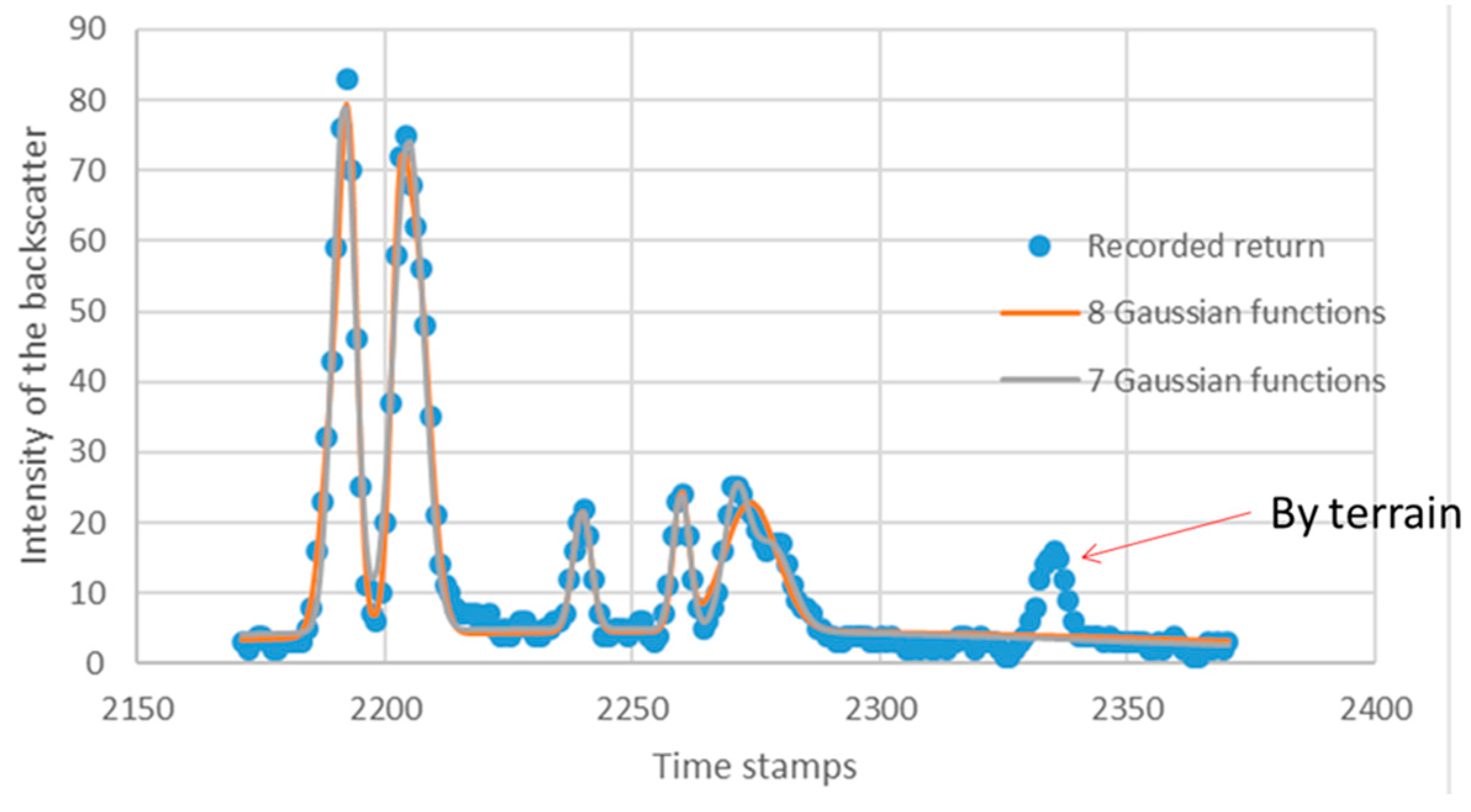
This new LiDAR instrument offers certain advantages for the DTM generation in dense vegetation over that recording discrete returns. Specifically, full-waveform systems store the whole signature of a returned radiation [14], so that advanced methods can be applied to detect weak echoes generated from terrain under vegetation canopies [15]. In addition, waveform parameters such as the pulse width and the backscatter cross-section can be used to improve the separation between terrain and vegetation canopies [16]. However, the classification of terrain points in a dense natural forest is still very difficult, even with the additional waveform parameters [16]. In 2009, Lin and Mills [17] proposed a novel routine to integrate the pulse width information to the progressive densification filter developed by Axelsson [18]. Their approach was demonstrated to be more effective in terms of the removal of low vegetation points and a more accurate DTM generation, compared with the traditional methods. Nonetheless, in their method [17], the pulse information was derived using a Gaussian decomposition method [19,20] before the integrated filtering process. To the best of the authors’ knowledge, all existing algorithms for the DTM generation from full-waveform data start their processing chains by decomposing signals to discrete returns (e.g., [21,22,23]). A problem with these methods is that weak echoes from the terrain may not be detected using a decomposition method, but they are very important to increase the DTM accuracy in densely vegetated terrain. To illustrate this issue, a recorded full-waveform of the return by a tree and the terrain underneath it is shown in Figure 1, where the echo generated by the terrain is marked. The function-fitting utility in Matlab was used to fit the full-waveform with a sum of Gaussian functions. Different numbers of Gaussian functions were tried. The best results in term of the residual error and visual inspection were achieved by fitting seven or eight Gaussian functions to the observations (Figure 1).
As expected, the “weak” echo generated by the terrain underneath the tree could not be detected. One may argue that the peak of the weak terrain echo may be detected based on the first and second derivative of the waveform. However, such an approach may lead to many false positives. Rigorous constraints are needed to filter out unwanted peaks. For example, in Xu et al., 2016 [24], initial echo components were first identified based on peak and inflection points in a full-waveform signal and then iteratively sifted based on a pre-determined energy term. This method was especially effective with overlapping echo components. In Ma et al., 2017 [25], an advanced optimization method, the grouping Levenberg-Marquardt (LM) algorithm, was used to fit the generalized Gaussian mixture function to a waveform. The grouping LM optimization method was demonstrated to be less sensitive to the initial parameters compared with the traditional one. Instead of using Gaussian functions, Salas et al. (2016, 2017) [26,27] introduced the new Moment Distance (MD) framework to characterize the canopy height based on the geometry and return power of the LiDAR waveform without having to go through curve modeling processes. Similarly, several studies in bathymetry used strategies in waveform decomposition considering there were usually two echoes with one from water surface and the other from the bottom [28,29].
In this study, we proposed an alternative method employing gained knowledge on the possible position of terrain to detect weak returns backscattered by the bare terrain and evaluate the benefit of their inclusion in the DTM generation. The developed method was validated using ground-measured elevations in a study area near Sault Ste. Marie, Ontario, Canada and demonstrated to generate accurate DTM.
2. Materials and Methods
2.1. Study Area and Data Used
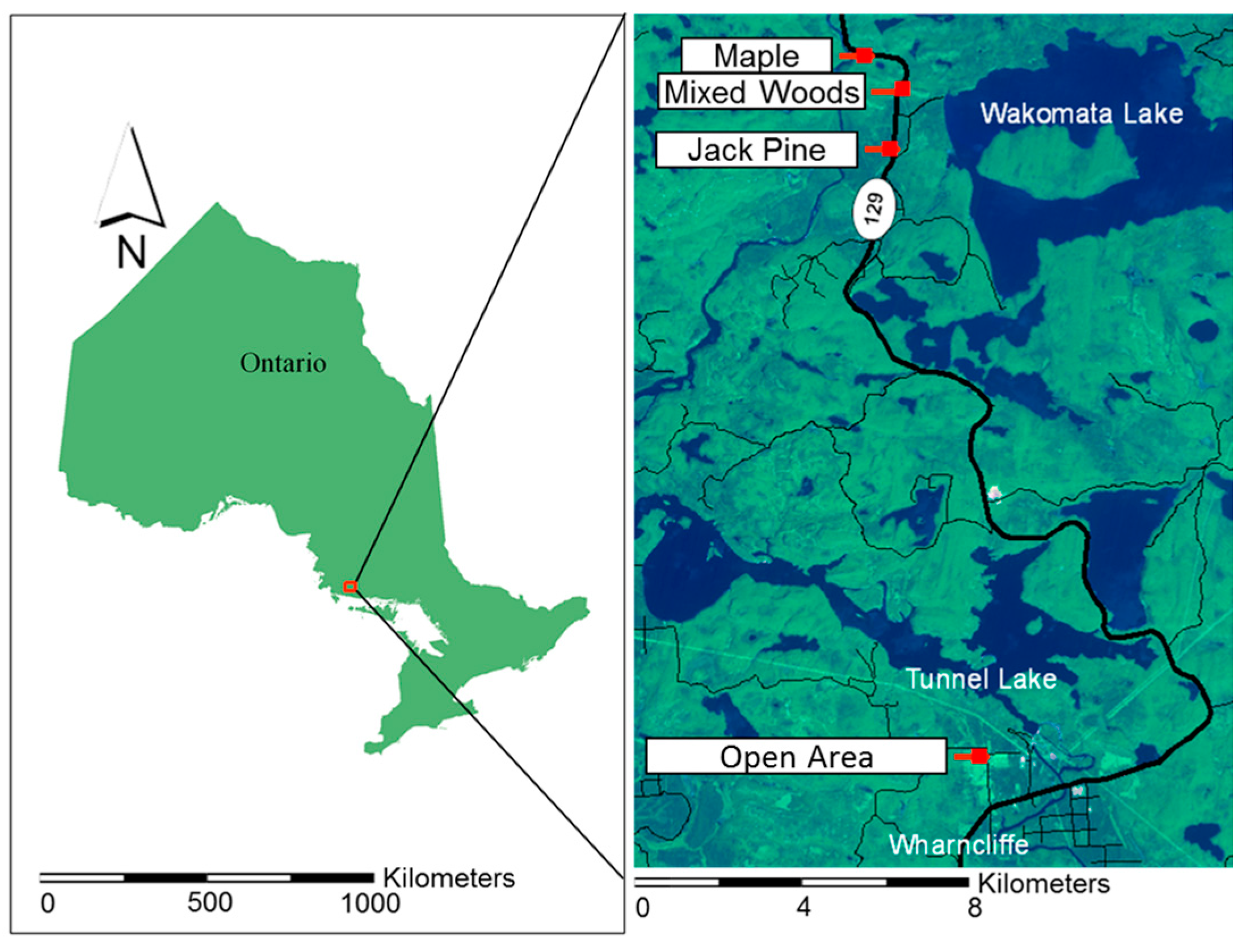
The study area is located in a Great Lakes-St. Lawrence forest region near Sault Ste. Marie, Ontario, Canada (46°33′56′′N, 83°25′18′′W), as shown in Figure 2. The terrain within the study area varies from 220 m to 440 m above the mean sea level and has a mild slope. The images of DTM and slope at a spatial resolution of 30 m by 30 m are shown in Figure 3. Four test sites, identified as Open Area, Maple, Mixed Woods, and Jack Pine, were selected and surveyed on the ground to validate the developed algorithm. The Open Area of the site features relatively flat terrain and sparse coverage with shrubs and spruce. Even though the terrain in the whole area is relatively flat, as shown in Figure 3, there are small rolling hills in the sites of Maple and Jack Pine and steep hills in the site of Mixed Woods. In the three forest sites (Maple, Jack Pine, and Mixed Woods), tree canopies are dense and closed, and maple, jack pine, and mixed coniferous and deciduous trees dominate, respectively.
The full-waveform LiDAR data used in this study were acquired in August 2009 over each site with a Riegl LMS Q-560 scanner mounted on an aircraft with an Applanix’ POS AV 310 system. The data were collected at the flight height of 150–300 m above the terrain by GeoDigital International (http://www.geodigital.com/) on two flight lines. The nominal footprint was approximately 10–20 cm. In addition to full-waveform data, the scanner also provided discrete data with a point density of 20 points per square meters (4 pulses per square meter). The ortho-views of the discrete LiDAR data of the four sites are shown in Figure 4, illustrating the canopy coverages in the study area.
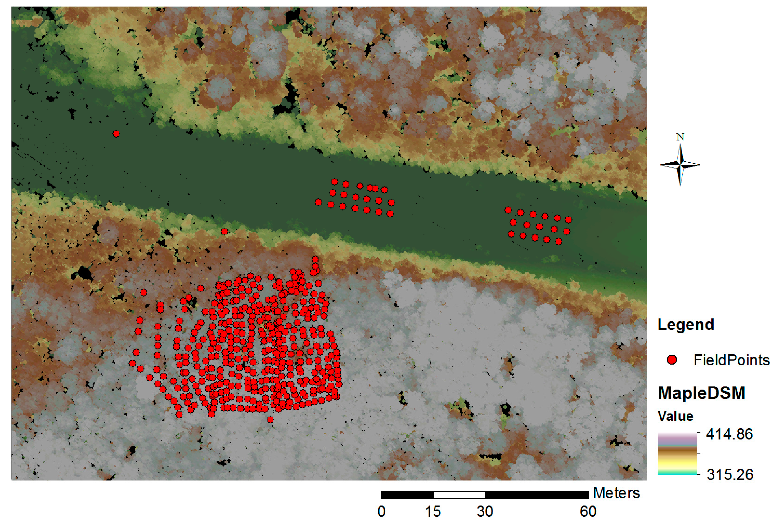
In order to validate the derived DTM, a ground surveying mission was introduced. Each study site was surveyed using relative static GPS positioning techniques and total station equipment within the designed geodetic network. Due to the labor intensity of ground survey operation, a subset of each site was selected, which was representative to the site and easy to access. Within each subset, one point was normally surveyed within 1 squared meter if logistically possible. The numbers of points surveyed were 301 (Open Area), 398 (Maple), 249 (Mixed Woods), and 327 (Jack Pine) for the four sites, respectively. In addition, a number of points on roads were also collected to help assess the horizontal accuracy of the LiDAR data. As an example, the layout of the collected points for the site of Maple is shown in Figure 5. The surveyed topographic points had accuracies of 4.33 cm horizontally and 3.57 cm vertically in heavily wooded areas and 3.67 cm horizontally and 2.22 cm vertically in open areas. The detailed procedures followed in the field and the results were provided in [30].
2.2. Methods
2.2.1. Overview
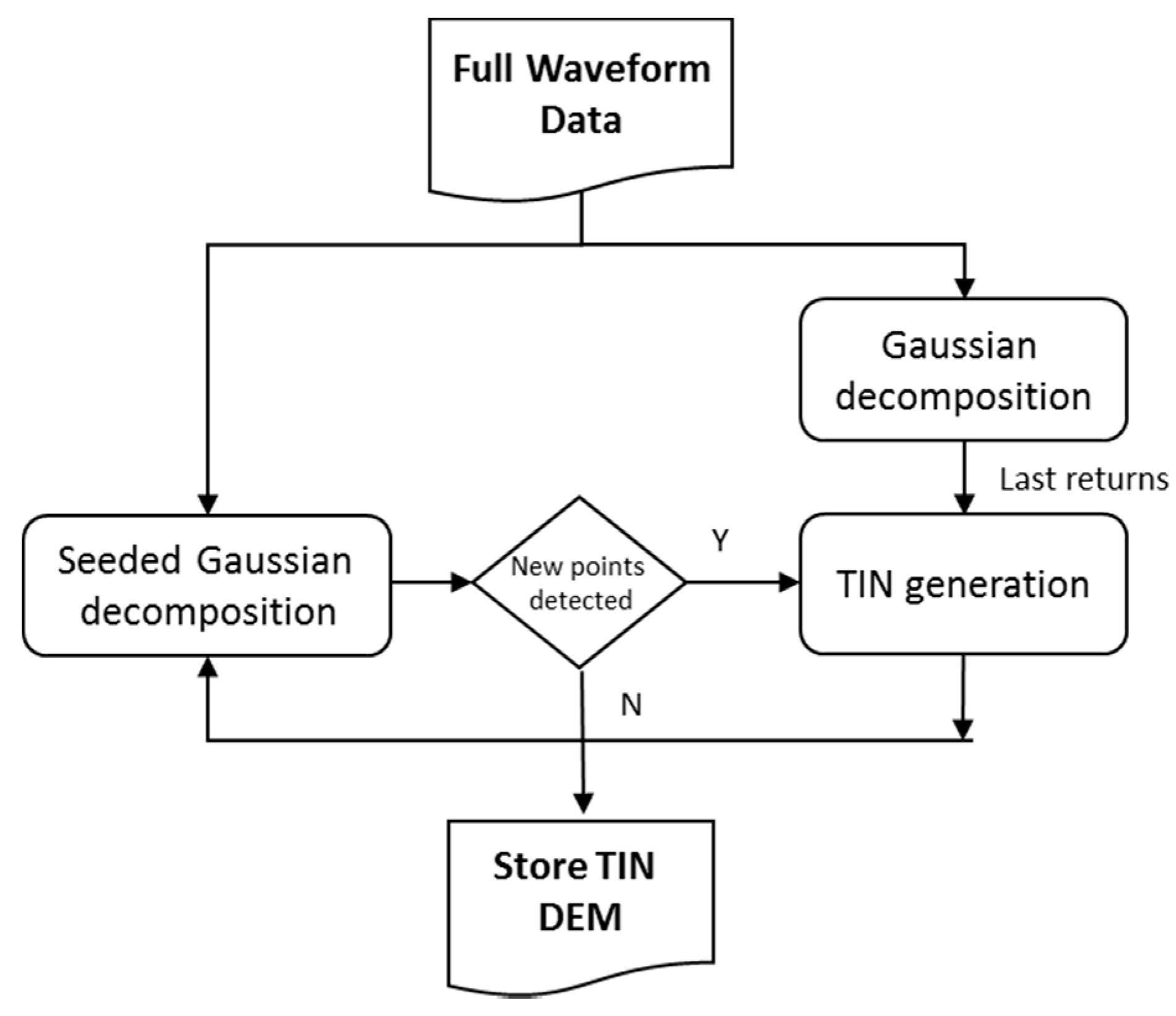
As illustrated in Figure 1 and discussed in Section 1, with a standard Gaussian decomposition method, weak returns generated by the terrain underneath trees are normally hard to detect. However, if one knows where the terrain would roughly be and thus where to look for a weak echo, the Gaussian decomposition could be constrained to a certain interval to detect the weak terrain echo. As a result, an integrated approach was proposed in this study to progressively carry out echo detection, identification of terrain points, and generation of triangular irregular network (TIN). As shown in the algorithmic diagram (Figure 6), with this method, each full-waveform was first decomposed into several discrete echoes using the Gaussian decomposition method [31,32]. A TIN model was then built from the terrain points and used to guide the detection of the weak echoes backscattered by the terrain but undetected by the Gaussian decomposition method. To do this, for any given TIN facet, the full-waveforms of the returns associated with the pulses passing through this TIN facet were examined near the surface for any terrain echoes. This process was identified as “seeded Gaussian decomposition” in Figure 6. The latest detected terrain points were used for the further iteration. These processes continued until no further terrain points were detected. In the following, the steps in the proposed method will be described in details.
2.2.2. Gaussian Decomposition
The Gaussian decomposition method [31,32] is commonly used to decompose the recorded full-waveform into several discrete echoes by fitting the Gaussian models, shown in Equation (1), to the recorded signal.
where is the number of the used Gaussian functions and was determined a prior to the decomposition, and , , and are the magnitude, central position, standard deviation (echo width) of the Gaussian function (echo) , respectively, that would be solved by minimizing the cost function (Equation (2)) using the Levenberg-Marquardt optimization method [15,33].
where is the number of samples in the recorded echo, and and are the magnitudes calculated by Equation (1) and measured at each sample point , respectively. For each waveform, only the samples whose amplitudes were greater than a threshold were used in the Gaussian decomposition. In this study, the method used in [34,35] was adopted, and the threshold T was set as three times the standard deviation of the noise, whose level in the data was estimated based on the recorded 15,000 samples of the emitted waveforms. For the LiDAR data used in this study, the standard deviation of the noise was estimated to be 3.5, and thus was set as 10.5. It is worth mentioning that was set to a higher value in this study to minimize the effect of the noise. A higher value might result in some weak echoes being overlooked, which was not an issue, since the weak echoes generated by terrain under vegetation canopies were detected in the subsequent steps. The number of Gaussian functions to be used to fit a given waveform was determined by the number of local maxima detected as zero-crossings toward the negative direction in the first-derivative of this waveform. The location and magnitude of the counted local maxima were used for the initial values of the Gaussian variables as well (Equation (1)). After Gaussian decomposition, the last or the only return of each waveform were identified and further examined to suppress any false returns caused by the so-called ringing effect [36,37], which is caused by the detection electronics of a LiDAR instrument when a strong backscatter signal is received. The delay between the true echo and its ringing copy lies typically within the range of 10 to 14 ns. In this study, based on experiments, a last return was considered to be an artifact caused by the ringing effect and removed if it trailed a strong return with a time delay between 10 to 14 ns and was 7 times weaker in the magnitude than the strong echo. The position, magnitude, and width of the remaining last returns or the only returns were recorded and used in the subsequent processes. A processing procedure was developed and implemented to geo-reference the locations of the detected LiDAR returns as well as each full-waveform signal using on board INS (Integrated Navigation System) data. It involved a series of coordinate transformation. Please refer to [30] for details.
2.2.3. TIN Generation
The progressive TIN method [18] was used in this study to construct the TIN representation of the DTM. A variation of the progressive TIN algorithm is also deployed as a module in the TerraSolid’s software: TerraScan [38]. The progressive TIN algorithm implemented in this study is a realization of TerraSolid’s ground extraction tool and was developed based on [18] and the information extracted from TerraScan’s User Guide. Starting from the lowest points in the neighborhoods with a pre-determined size, an initial TIN model was then constructed. During each iteration, all the points were evaluated against the TIN using the following threshold parameters: iteration angle, iteration distance, and terrain angle, all of which were user-defined. The iteration angle threshold was the maximum accepted value for an angle that was computed between the candidate terrain point, the closest vertex of the TIN, and candidate point’s projection onto the surface of the TIN facet (angle is labelled in Figure 7). The iteration distance threshold was the maximum allowable distance (in magnitude) of the normal vector computed between the TIN facet to the candidate point (labelled in Figure 7). The third and final threshold parameter used was the terrain angle, which was the threshold for the slopes of the three new TIN facets that form as a result of the addition of the candidate point. If a candidate point satisfied all three thresholds, it was accepted by the TIN model. Once all the points were evaluated, the new vertices were added to the TIN model. The algorithm ran until there were no new points to be added to the model or until fewer points than a preset threshold were introduced into the model, producing a TIN model ready to be used in the seeded Gaussian decomposition. For the study area, the maximum iteration angle and distance were set to 6 degrees and 1.4 m, respectively, and the maximum resulting terrain angle was chosen to be 80 degrees. These values were determined experimentally. The algorithm was implemented using CGAL (Computational Geometry Algorithm Library, http://www.cgal.org/). Triangulation was done via Delaunay triangulation in CGAL. The implemented progressive TIN generation was also applied to the discrete LiDAR data provided by the laser scanner (together with the full-waveform signals) and the generated DTMs were compared with those obtained by the proposed method (Figure 6).
2.2.4. Seeded Gaussian Decomposition
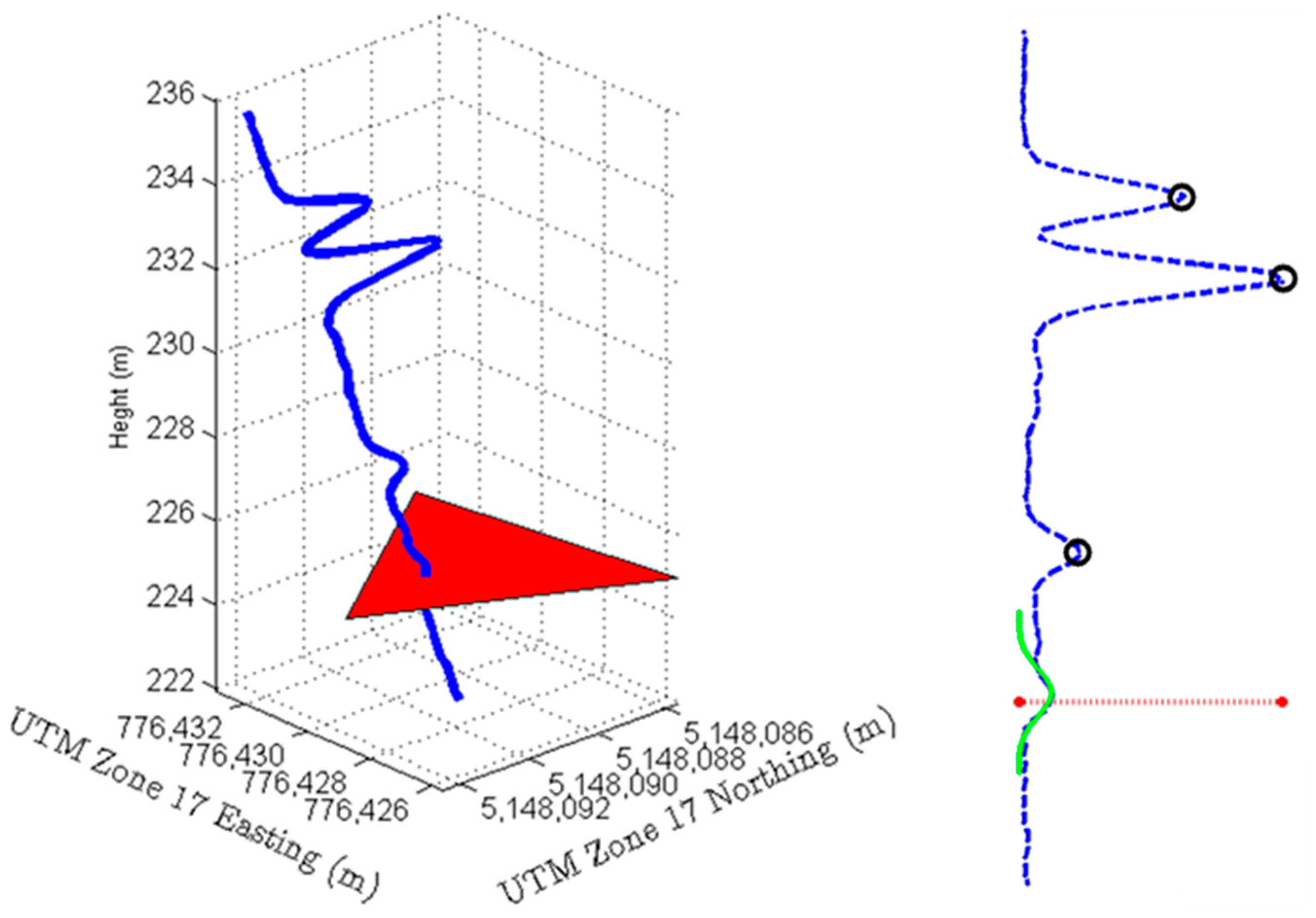
Every facet of the TIN model, obtained from the progressive TIN algorithm, was treated as a plane. Its equation was determined by its three vertices. To determine which waveforms passed a particular facet, each waveform was represented as a line defined by the point of origin (X0, Y0, Z0) where the laser scanner was located and the unit direction vector to which the emitted pulse pointed. For a given facet, if a waveform was found to intersect with this facet by solving the line and plane equations, the location on the waveform where the laser pulse intersected with the facet was used as the seed to assist the Gaussian decomposition. If no waveform passed through a given facet, the process moved on to next facet. As an example, one of the laser pulses passing through the red facet in the TIN model along with its full-waveform return is shown in Figure 8.
For the waveform in Figure 8, three returns were detected (blue dashed line with circle marking the peak) using the typical Gaussian decomposition method described above. These returns were backscattered from a tree. The red dashed line shows the location of the intersection of the facet and the waveform. The intersection location was used as a seed to initiate a fitting of a Gaussian function near the seed, which generated additional return (green curve). The seeded Gaussian decomposition was similar to the typical Gaussian decomposition method described previously with the seeded region (approximately one meter in either direction from the estimated terrain level) evaluated from right to left in order to locate the cluster of points that best resembled a return pulse (green line in Figure 8). The rightmost maxima point in the seeded region was then identified as a first point of a segment to be fitted. The segment was grown recursively starting from the maxima point and expanded in both directions to include all the samples that were less in the amplitude than the samples added in a previous iteration. If the total length on the segment satisfied the minimum point requirement (7 samples minimum due to the larger noise effects associated with the lower amplitude pulses), the Gaussian fitting was performed on the extracted segment to fit one return only. If the fitted echo was not caused by ringing effect, the position of the echo was geo-referenced and then included into the dataset. Otherwise, the next candidate cluster in the seeded region (going right to left) was evaluated. After the process of seeded Gaussian decomposition, a number of new candidate terrain points were detected. These new candidate points were fed back into the module of “TIN generation” (Figure 6) and the previously built TIN was modified. If there were no more new points detected with the aid of the seeds, the latest TIN terrain model was stored as the final DTM. In general, two iterations were sufficient for vast majority of the discernible low amplitude echoes to be included into the DTM.
2.2.5. Validation
To validate the effectiveness of the proposed method, several quantitative measures were employed. As mentioned earlier, the elevations of a series of points in each study site were measured using traditional surveying methods (Section 2.1). For each surveyed point, the LiDAR-derived elevation was calculated from its corresponding TIN facet in the generated DTM. Both the DTMs generated by the proposed and progressive TIN methods were evaluated. The correlation coefficients between the ground-measured and LiDAR-derived elevations were calculated and a Fisher’s z-test was applied to evaluate whether the correlation coefficients corresponding to the proposed and progressive TIN methods were significantly different. Let the population correlation coefficients in elevations between the ground-measured and those derived from the progressive TIN and developed methods be and , respectively; their corresponding sample correlation coefficients and ; and the sample size . The null and alternative hypothesis for the Fisher’s z-test was ; . The z-statistics was calculated by Equation (3). At the significant level of 0.05, the critical value is 1.96. If the calculated z-value was smaller than 1.96, the null hypothesis was accepted, otherwise, the alternative hypothesis was accepted.
In addition, the basic statistics of the differences between the LiDAR-derived and the ground-measured elevations were calculated, such as the minimum, maximum, mean, standard deviation, and RMSE. An F-test was employed to evaluate the ratio of two variances for their homogeneity, here specifically about whether the proposed method had a smaller RMSE in comparison with the progressive TIN method. Let the population mean squared error of those elevations derived from the progressive TIN and developed methods be and , respectively; their corresponding estimated values as and with the sample size which are materialized by using the elevation differences from two methods against the ground measured values as their references. The null and alternative hypothesis for the Fisher’s F-test was ; . The F-statistics was calculated as F = . At the significantly level of 0.05 for the sample size at 200, the critical value is 1.26. Because the sample sizes were over 200 for all of four sites; the critical value for each case was smaller than 1.26. If the calculated F-value was smaller than 1.26, the null hypothesis was accepted, otherwise, the alternative hypothesis was accepted. For the details of the hypothesis tests, please refer to [39,40].
3. Results
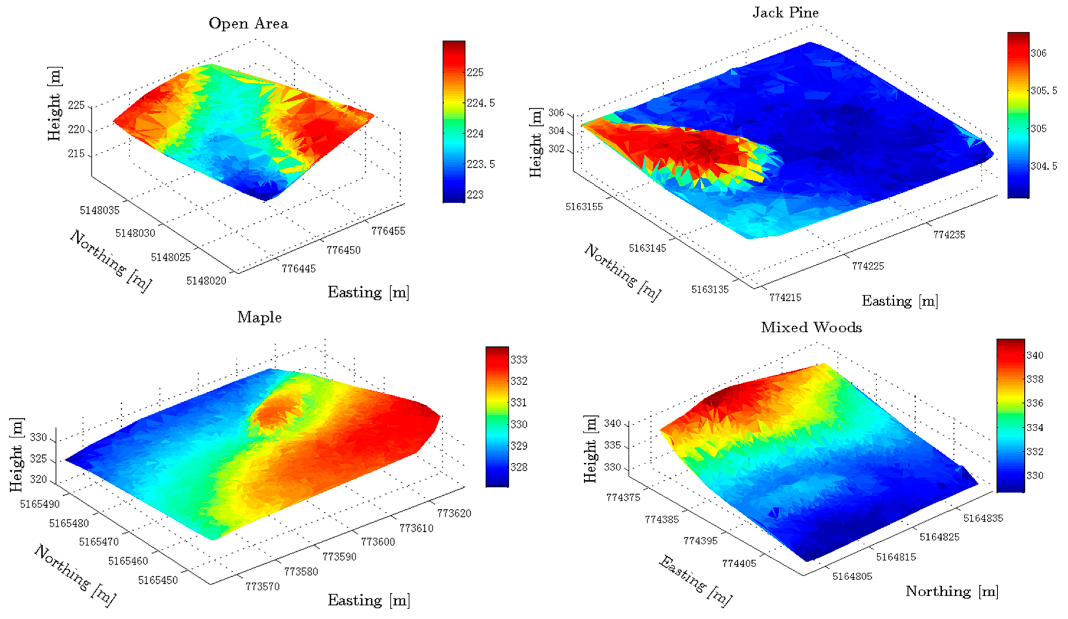
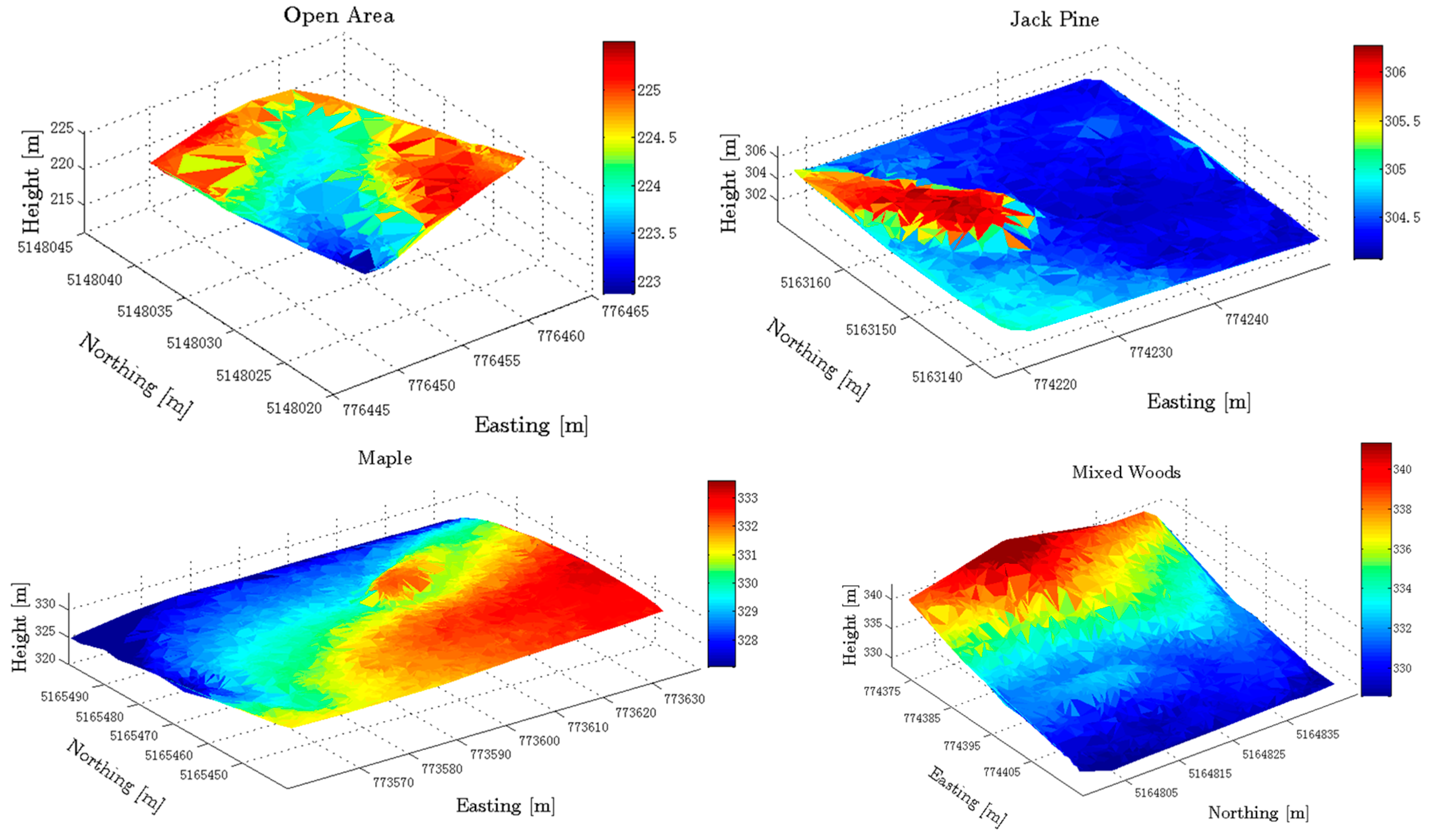
The generated DTMs for the study sites are shown in Figure 9. For comparison, the DTMs generated using the progressive TIN method described in Section 2.2.3 are shown in Figure 10. By observing the presented DTMs, more details can be seen from the ones generated by the proposed algorithm. Obviously, the additional terrain points detected using the novel integrated algorithm provided a better definition of the shapes of the mounds. As shown in Table 1, on average the number of the terrain points per square meter detected by the developed algorithm was bigger than the one by the progressive TIN method.
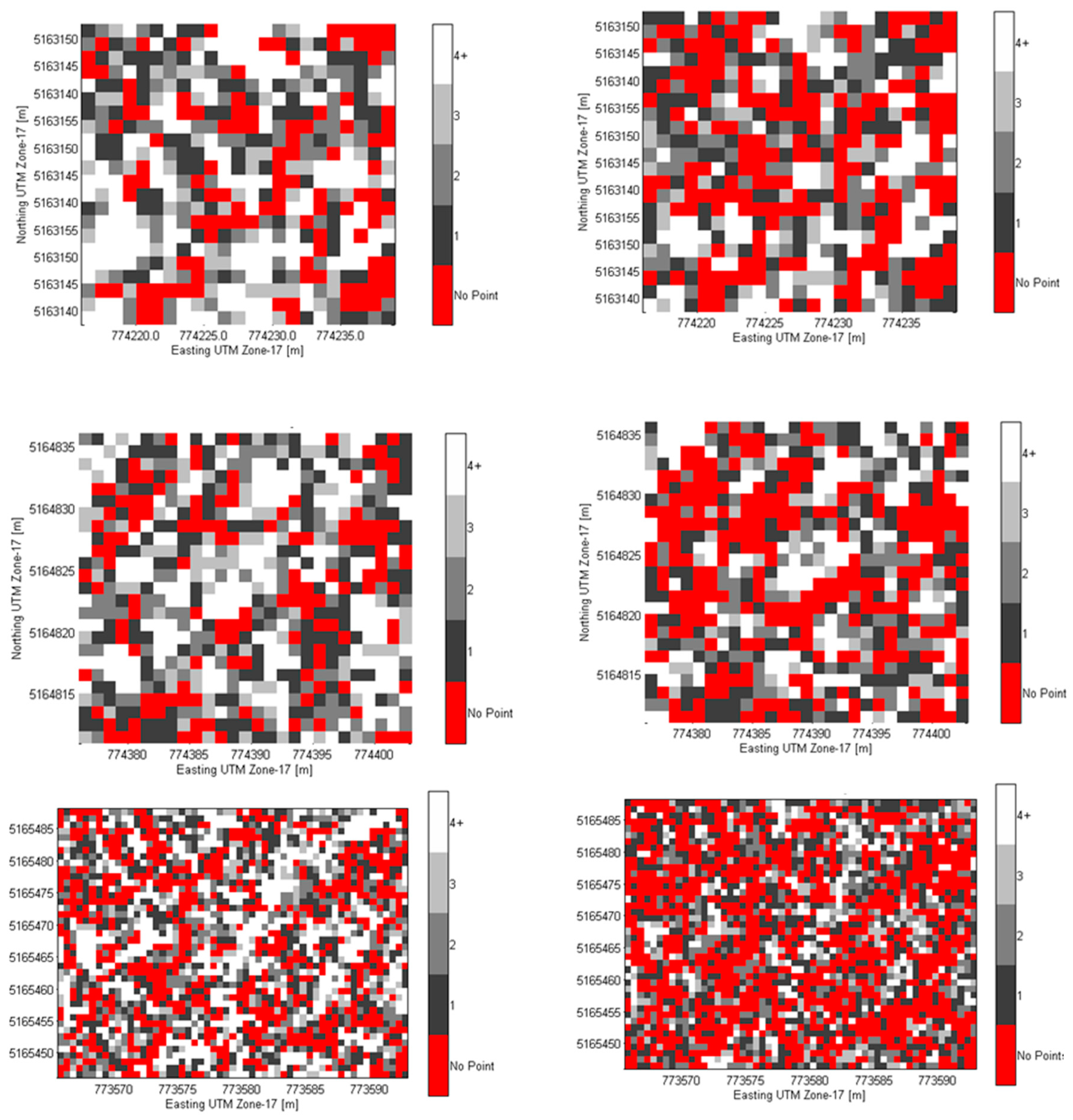
To examine how the increased terrain points affect DTM generation, each test site was assigned a one-by-one meter grid and the number of points that fell within each grid cell was calculated. A ratio of the number of cells containing at least one point to the total number of cells was computed for each site to provide the information on coverage of the derived terrain model as the visualization of the grid demonstrated the distribution of gaps in coverage. Figure 11 displays the results of this analysis for all the study sites generated using both the proposed novel iterative algorithm and the progressive TIN method. The plots in Figure 11 demonstrated that the novel DTM extraction method systematically had a better point coverage than that of the DTMs obtained by the progressive TIN method. This overall improvement in coverage could be more beneficial for terrain reconstruction than the detection of a large number of points in areas that already had ground points detected. By minimizing gaps in coverage, there was a greater probability of detecting terrain variations that could have been missed otherwise, and therefore a more accurate representation of the terrain could be obtained as a result.
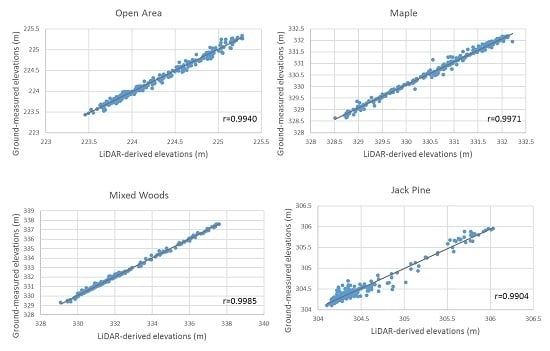
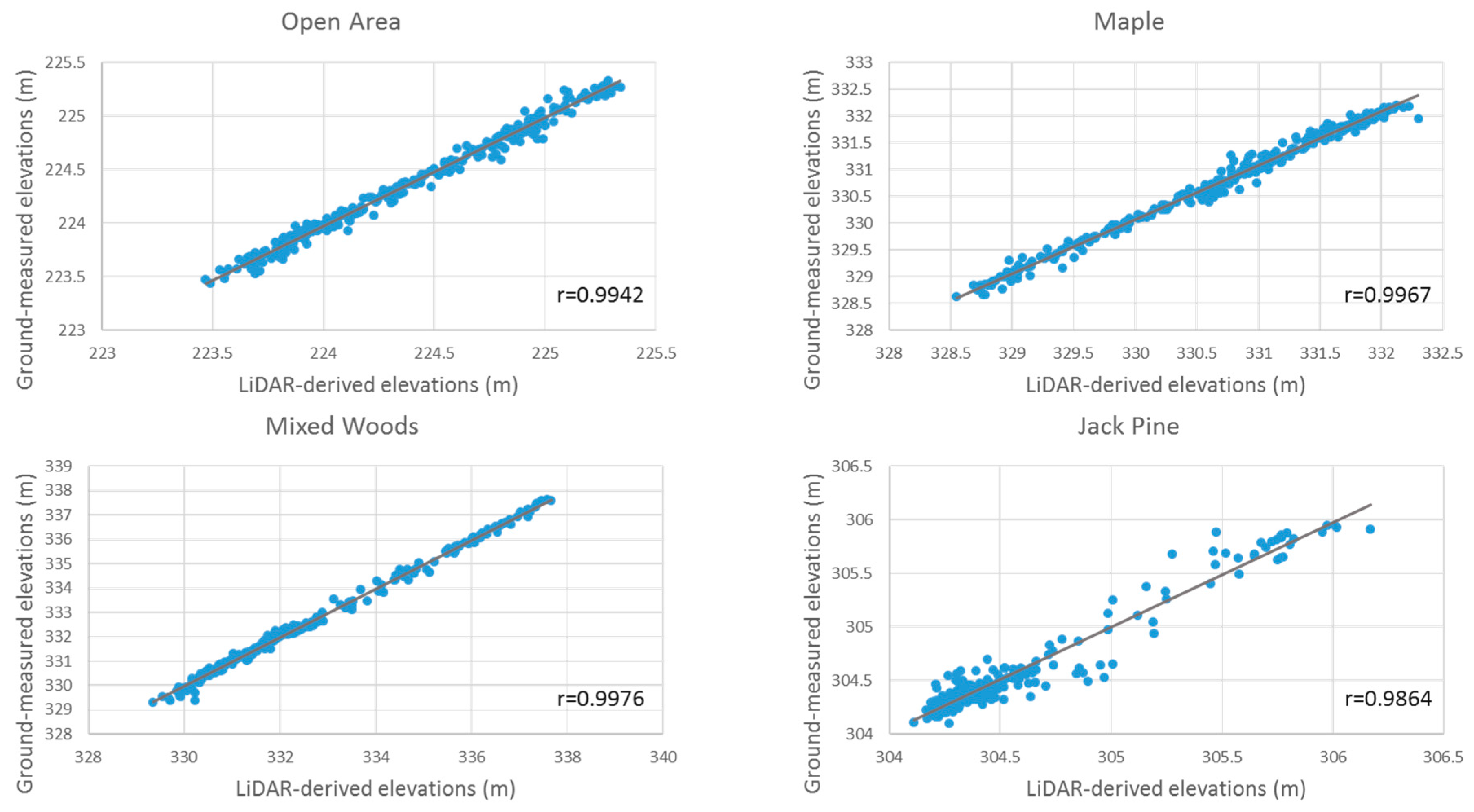
The scattering plots between the LiDAR-derived elevations generated by the developed method and by the progressive TIN method vs. the ground-measured elevations for the four study sites are shown in Figure 12 and Figure 13, respectively. The results from the Fisher’s z-test on the correlation coefficients are summarized in Table 2. The statistical summary about the differences between the LiDAR-derived and the ground-measured elevations is given in Table 3.
4. Discussion
As shown in Table 1 and Figure 11, with the developed method, the number of terrain points detected was increased. This increase in the number of the terrain points was contributed by the detected weak echoes that were back-scattered by the terrain underneath vegetation. For the Maple site with dense deciduous canopies present, some laser pulses could pass through within-crown gaps and were reflected back by the terrain as the weak echoes, which could not be normally detected by the current available processing methods. For other sites, a number of the evergreen trees exited. These coniferous trees with few within-crown gaps allowed relatively few LiDAR pulses travelling through and thus few returns were generated by the underneath terrain. Furthermore, thick underbrush existed in the sites of Jack Pine and Open Area, which could further impede the LiDAR penetration to ground. As reviewed in Section 1, several advanced methods [9,10,11,12,13] were reported in the literature to generate more reliable terrain points for a given set of discrete points using local properties. These methods can be used together with the proposed method to further filter out falsely identified terrain points. A further discussion will be provided in the next paragraph. The proposed method provided an alternative way to improve the decomposition of a full-waveform signal. Different from the newly emergent methods [24,25,26], this method used an iteratively built terrain model to guide the process of full-waveform decomposition and was not sensitive to the initial values.
By comparing the DTMs generated from the developed algorithm (Figure 12) and those from the progressive TIN method (Figure 13) for the four study sites, one can see that the sites of Maple and Open Area achieved similar accuracies. For the sites of Jack Pine and Mixed Woods, the developed algorithm reached better results in predicting surface elevations demonstrated by the higher correlation coefficients. The Fisher’s z-test (Table 3) demonstrated that the differences in the correlation coefficients obtained by these two methods were significant at the significant level of 0.05. For the Open Area site, the terrain was relatively flat and even with a few of the terrain points, a high accurate DTM could be achieved. Both the progressive TIN and the developed methods generated similar results as indicated by the similar correlation coefficients. For other sites, some small mounds were observed during field inspection and some points were collected around these mounds. As mentioned in Section 2.1, 398, 249, and 327 points were surveyed on the ground for the sites of Maple, Mixed Woods, and Jack Pine, respectively. Among the large number of surveyed points (398) in the Maple site, most of them lied on the relatively flat terrain. As a result, the accuracy improvement in this site was not as significant as in the sites of Mixed Woods and Jack Pine. Similarly, the RMSE and F-test results in Table 3 showed that the proposed method generated higher accurate DTMs compared with the progressive TIN method for the sites of Jack Pine and Mixed Woods at the significant level of 0.05. For the sites of Maple and Open Area, the two methods generated similar results. The F-test was also applied to the standard deviations of the differences. For the sites of Open Area and Maple, the standard deviations related to the two methods were similar, while the standard deviation for the progressive TIN method was significantly larger than the one for the proposed method for the sites of Jack Pine and Mixed Woods. Examining the mean values of the differences between the ground-measured and LiDAR-derived elevations reveals that the developed method tended to underestimate the elevation. This might be because that weak echoes caused by noise were falsely taken as those detected by terrains. A better filtering methods, such as those proposed in [9,10,11,12,13] may help to remove false terrain points. It is worth mentioning that noise might be introduced by adding the weak echoes, which might negatively affect the accuracy of the generated DTM, especially in the flat areas. In the future study, a cost-benefit analysis may be necessary to evaluate how much point position accuracy can be sacrificed in order to extract additional terrain features. This decision-making process would subdivide the scanned area into zones and identify areas that would benefit from having additional point coverage. This would assist in determining where the inclusion of the lower amplitude pulses would benefit the terrain extraction and where it would be detrimental to quality of the derived DTM. There certainly is a need to monitor the accuracy of the derived points, and to have an error value assigned to the coordinates of each point extracted from the LiDAR waveform.
Based on the 1275 (301 + 398 + 249 + 327) points surveyed in four study sites across this study area, the estimated elevations using the developed method had a strong linear relationship with the measured ones with r above 0.99 and the RMSEs between them were less than 0.15 m even for areas with hilly terrains underneath vegetation canopies. Such an accuracy can normally be achieved for open and hard surface [5]. The reported accuracies in [5] might be improved by using the advanced filtering methods in [9,10,11,12,13]. As mentioned earlier, this developed method can be employed together with these new filtering methods to improve DTM generated as well, which will be investigated in future studies.
5. Conclusions
In this study, an integrated approach was developed to improve the DTM generation in the vegetated area by detecting the weak pulses (with low amplitudes) generated from the terrain under trees, which could not be detected by the commonly used Gaussian fitting. Our results show that in heavily forested areas, the extraction of low amplitude return pulses from full-waveform LiDAR signatures provided a denser point sampling of the terrain in comparison with the commercially available methodology which was shown to be instrumental to improving the quality of the derived terrain model.
The point distribution and density plots (Figure 11) demonstrated the consistent improvements in point coverage of the derived DTM when one compares the developed algorithm with the progressive TIN method. For areas containing hilly terrain, the increased point coverage leads to a more accurate modeling of the terrain variations and thus a more accurate representation of the ground surface. It is visible from the DTMs generated using the developed algorithm for the sites of Maple, Mixed Woods, and Jack Pine (Figure 9 and Figure 10) that the addition of weak echoes backscattered by the terrain underneath vegetation canopies provided detailed characterization of the variable terrain in these sites. Statistical analysis carried out on elevations of more than 1000 points demonstrated that the elevations estimated from the developed methods had a strong linear relationship with ground-measured ones with correlation coefficients above 0.99 and the RMSEs between them were less than 0.15 m even for areas with hilly terrains underneath vegetation canopies. For the sites of Mixed Woods and Jack Pine, the correlation coefficients were significantly higher and the RMSEs were lower than those with the existing progressive TIN method at the significant level of 0.05. The site of Open Area and Maple featuring a flat terrain did not benefit from the introduction of the weak echoes. In this study, the evaluation of this developed method was carried out based on ground-measured elevations. In future work, we will extend the validation to some of the end-products of DTM. We will assess the performance of our method in the analysis of specific geomorphic features.
Acknowledgments
The authors are grateful for financial support provided by the Natural Sciences and Engineering Research Council (NSERC) of Canada, the Canadian Space Agency, and GeoDigital, Inc. We would like the acknowledge Ontario Ministry of Natural Resources for the 30 m by 30 m DTM data.
Author Contributions
B. Hu, D. Gumerov, and J. Wang conceived and designed the experiments. D. Gumerov performed the experiments and analyzed the data under the guidance of B. Hu and J. Wang. W. Zhang contributed data analysis. B. Hu wrote the paper with the contributions from other co-authors.
Conflicts of Interest
The authors declare no conflict of interest.
References
- Gonga-Saholiariliva, N.; Gunnell, Y.; Petit, C.; Mering, C. Techniques for quantifying the accuracy of gridded elevation models and for mapping uncertainty in digital terrain analysis. Prog. Phys. Geogr. 2011, 35, 739–764. [Google Scholar] [CrossRef]
- Liu, X. Airborne LiDAR for DEM generation: Some critical issues. Prog. Phys. Geogr. 2008, 32, 31–49. [Google Scholar]
- Glennie, C. Rigorous 3D error analysis of kinematic scanning LiDAR systems. J. Appl. Geod. 2007, 1, 147–157. [Google Scholar] [CrossRef]
- Baltsavias, E.P. Airborne laser scanning: Existing systems and firms and other resources. ISPRS J. Photogramm. Remote Sens. 1999, 54, 165–198. [Google Scholar] [CrossRef]
- Su, J.; Bork, E. Influence of vegetation, slope, and LiDAR sampling angle on DEM accuracy. Photogramm. Eng. Remote Sens. 2006, 72, 1265–1274. [Google Scholar] [CrossRef]
- Hodgson, M.E.; Bresnahan, E. Accuracy of airborne LiDAR-derived elevation: Empirical assessment and error budget. Photogramm. Eng. Remote Sens. 2004, 70, 331–339. [Google Scholar] [CrossRef]
- Tinkham, W.T.; Huang, H.; Smith, A.M.S.; Shrestha, R.; Falkowski, M.J.; Hudak, A.T.; Link, T.E.; Glenn, N.F.; Marks, D.G. A comparison of two open source LiDAR surface classification algorithms. Remote Sens. 2011, 3, 638–649. [Google Scholar] [CrossRef]
- Tinkham, W.T.; Smith, A.M.S.; Hoffman, C.M.; Hudak, A.T.; Falkowski, M.J.; Swanson, M.E.; Gessler, P.E. Investigating the influence of LiDAR ground surface errors on the utility of derived forest inventories. Can. J. For. Res. 2012, 42, 413–422. [Google Scholar] [CrossRef]
- Maguya, A.S.; Junttila, V.; Kauranne, T. Adaptive algorithm for large scale dtm interpolation from LiDAR data for forestry applications in steep forested terrain. ISPRS J. Photogramm. Remote Sens. 2013, 85, 74–83. [Google Scholar] [CrossRef]
- Su, W.; Sun, Z.; Zhong, R.; Huang, J.; Li, M.; Zhu, J.; Zhang, K.; Wu, H.; Zhu, D. A new hierarchical moving curve-fitting algorithm for filtering LiDAR data for automatic DTM generation. Int. J. Remote Sens. 2015, 36, 3616–3635. [Google Scholar] [CrossRef]
- Hu, X.; Ye, L.; Pang, S.; Shan, J. Semi-global filtering of airborne LiDAR data for fast extraction of digital terrain models. Remote Sens. 2015, 7, 10996–11015. [Google Scholar] [CrossRef]
- Zhang, J.; Lin, X. Filtering airborne LiDAR data by embedding smoothness-constrained segmentation in progressive TIN densification. ISPRS J. Photogramm. Remote Sens. 2013, 81, 44–59. [Google Scholar] [CrossRef]
- Zhang, W.M.; Qi, J.B.; Wan, P.; Wang, H.T.; Xie, D.H.; Wang, X.Y.; Yan, G.J. An Easy-to-Use Airborne LiDAR Data Filtering Method Based on Cloth Simulation. Remote Sens. 2016, 8, 501. [Google Scholar] [CrossRef]
- Mallet, C.; Bretar, F. Full-waveform topographic LiDAR: State-of-the-art. ISPRS J. Photogram. Remote Sens. 2009, 64, 1–16. [Google Scholar] [CrossRef]
- Chauve, A.; Mallet, C.E.; Bretar, F.E.E.; Durrieu, S.; Deseilligny, M.P.; Puech, W. Processing full-waveform LiDAR data: Modeling raw signals. Int. Arch. Photogramm. Remote Sens. Spat. Inf. Sci. 2007, 36, 102–107. [Google Scholar]
- Wagner, W.; Hollaus, M.; Briese, C.; Ducic, V. 3D vegetation mapping using small-footprint full-waveform airborne laser scanners. Int. J. Remote Sens. 2008, 29, 1433–1452. [Google Scholar] [CrossRef]
- Lin, Y.-C.; Mills, J.P. Integration of full-waveform information into the airborne laser scanning data filtering process. Int. Arch. Photogramm. Remote Sens. Spat. Inf. Sci. 2009, 38, 224–229. [Google Scholar]
- Axelsson, P. DEM generation from laser scanner data using adaptive TIN models. Int. Arch. Photogramm. Remote Sens. 2000, 33, 110–117. [Google Scholar]
- Lin, Y.-C.; Mills, J.P.; Smith-Voysey, S. Detection of weak and overlapping pulses from waveform airborne laser scanning data. In Proceedings of the SilviLaser, Edinburgh, UK, 17–19 September 2008; pp. 478–487. [Google Scholar]
- Reitberger, J.; Krzystek, P.; Stilla, U. Analysis of full-waveform LiDAR data for the classification of deciduous and coniferous trees. Int. J. Remote Sens. 2008, 29, 1407–1431. [Google Scholar] [CrossRef]
- Doneus, M.; Briese, C. Digital terrain modelling for archaeological interpretation within forested areas using full-waveform laser scanning. In Proceedings of the 7th International Symposium on Virtual Reality, Archaeology and Cultural Heritage (VAST), Nicosia, Cyprus, 30 October–4 November 2006. [Google Scholar]
- Goncalves, G.; Pereira, L. Assessment of the performance of eight filtering algorithms by using LiDAR data of unmanaged eucalypt forest. In Proceedings of the Silvilaser 2010: The 10th International Conference on LiDAR Applications for Assessing Forest Ecosystems, Freiburg, Germany, 14–17 September 2010. [Google Scholar]
- Mandlburger, G.; Briese, C.; Pfeifer, N. Progress in LiDAR sensor technology—Chance and challenge for DTM generation and data administration. In Proceedings of the 51th Photogrammetric Week, Stuttgart, Germany, 3–7 September 2007. [Google Scholar]
- Xu, L.; Duan, L.; Li, X. A high success rate full-waveform LiDAR echo decomposition method. Meas. Sci. Technol. 2016, 27, 015205. [Google Scholar] [CrossRef]
- Ma, H.; Zhou, W.; Zhang, L.; Wang, S. Decomposition of small-footprint full waveform LiDAR data based on generalized Gaussian model and grouping LM optimization. Meas. Sci. Technol. 2017, 28, 045203. [Google Scholar] [CrossRef]
- Salas, E.A.L.; Henebry, G.M. Canopy Height Estimation by Characterizing Waveform LiDAR Geometry Based on Shape-Distance Metric. AIMS Geosci. 2016, 2, 366–390. [Google Scholar] [CrossRef]
- Salas, E.A.L.; Amatya, S.; Henebry, G.M. Application of Iterative Noise-adding Procedures for Evaluation of Moment Distance Index for LiDAR Waveforms. AIMS Geosci. 2017, 3, 187–215. [Google Scholar] [CrossRef]
- Wang, C.; Li, Q.; Liu, Y.; Wu, G.; Liu, P.; Ding, X. A comparison of waveform processing algorithms for single-wavelength LiDAR bathymetry. ISPRS J. Photogramm. Remote Sens. 2015, 101, 22–35. [Google Scholar] [CrossRef]
- Pan, Z.; Glennie, C.; Hartzell, P.; Fernandez-Diaz, J.; Legleiter, C.; Overstreet, B. Performance Assessment of High Resolution Airborne Full Waveform LiDAR for Shallow River Bathymetry. Remote Sens. 2015, 7, 5133–5159. [Google Scholar] [CrossRef]
- Gumerov, D. DTM Generation in Forested Areas from Full-Waveform Airborne LiDAR Data. Master’s Thesis, York University, Toronto, ON, Canada, 20 November 2014. [Google Scholar]
- Hofton, M.; Minster, J.; Blair, J. Decomposition of laser altimeter waveforms. IEEE Trans. Geosci. Remote Sens. 2000, 38, 1989–1996. [Google Scholar] [CrossRef]
- Wagner, W.; Ulrich, A.; Ducic, V.; Melzer, T.; Studnicka, N. Gaussian decomposition and calibration of a novel small-footprint full-waveform digitising airborne laser scanner. ISPRS J. Photogram. Remote Sens. 2006, 60, 100–112. [Google Scholar] [CrossRef]
- Jutzi, B.; Stilla, U. Measuring and processing the waveform of laser pulses. In Proceedings of the 7th Optical 3-D Measurement Techniques, FIG/IAG/ISPRS, Vienna, Austria, 3–5 October 2005; pp. 194–203. [Google Scholar]
- Stilla, U.; Jutzi, B. Waveform analysis for small-footprint pulsed laser systems. In Topographic Laser Ranging and Scanning: Principles and Processing; Shan, J., Toth, C.K., Eds.; CRC Press: Boca Raton, FL, USA, 2008; pp. 215–234. [Google Scholar]
- Lin, Y.C.; Mills, J.P.; Smith-Voysey, S. Rigorous pulse detection from full-waveform airborne laser scanning data. Int. J. Remote Sens. 2010, 31, 1303–1324. [Google Scholar] [CrossRef]
- Roncat, A.; Wagner, W.; Melzer, T.; Ullrich, A. Echo detection and localization in full-waveform airborne laser scanner data using the averaged square difference function estimator. Photogramm. J. Finl. 2008, 21, 62–75. [Google Scholar]
- Magruder, L.A.; Neuenschwander, A.L. LiDAR full-waveform data analysis for detection of faint returns through obscurants. In Proceedings of the SPIE 7323; Turner, M.D., Kamerman, G.W., Eds.; SPIE: Bellingham, WA, USA, 2009; Volume 7323. [Google Scholar]
- Soininen, A. Terrascan User’s Guide. Terrasolid: Helsinki, Finland; Available online: http://www.terrasolid.com/download/user_guides.php (accessed on 30 May 2017).
- Wackerly, D.D.; Mendenhall, W., III; Scheaffer, R.L. Mathematical Statistics with Applications, 7th ed.; Cengage Learning, Inc.: Belmont, CA, USA, 2008. [Google Scholar]
- Bartoszynski, R.; Niewiadomska-Bugaj, M. Probability and Statistical Inference, 2nd ed.; John Wiley & Sons Inc.: Hoboken, NJ, USA, 2007. [Google Scholar]
Figure 1.
An example of a returned full-waveform of a laser pulse passing through a tree (blue points), the modelled ones by fitting the summation of eight and seven Gaussian functions to whole waveform (orange and grey lines, respectively). The echo generated by the terrain is pointed by the red arrow.

Figure 2.
The location of the study area (left panel) and the plots for validation (right panel).

Figure 3.
(a) Digital elevation model of the study area at the spatial resolution of 30 m by 30 m. (b) The slope calculated from the digital elevation model in (a).
Figure 3.
(a) Digital elevation model of the study area at the spatial resolution of 30 m by 30 m. (b) The slope calculated from the digital elevation model in (a).

Figure 4.
The ortho-views of the discrete LiDAR data of the four forest sites.

Figure 5.
The topographic points collected in the field in the Maple site and on a road that were used as references to assess the horizontal accuracy of LiDAR points and to validate the generated DTM using the proposed method, overlain on the digital surface model generated from the LiDAR data.
Figure 5.
The topographic points collected in the field in the Maple site and on a road that were used as references to assess the horizontal accuracy of LiDAR points and to validate the generated DTM using the proposed method, overlain on the digital surface model generated from the LiDAR data.

Figure 6.
The diagram of the developed method.

Figure 7.
Progressive triangular irregular network (TIN) algorithm parameters: θ, the iteration angle and D, the iteration distance, P is the point to be tested, and A, B, and C are the TIN facet vertices.
Figure 7.
Progressive triangular irregular network (TIN) algorithm parameters: θ, the iteration angle and D, the iteration distance, P is the point to be tested, and A, B, and C are the TIN facet vertices.

Figure 8.
Left panel: A recorded waveform passing through a facet of the terrain TIN model. Right Panel: The black circles are the peaks of the returns detected by the typical Gaussian decomposition method. The red line shows the location of the seed (point of intersection of the waveform and the TIN facet) used for the seeded Gaussian decomposition, and the green curve is the result of fitting one Gaussian function to the region near the seed.

Figure 9.
The TIN representation of the generated digital terrain model (DTM) models using the developed algorithm.
Figure 9.
The TIN representation of the generated digital terrain model (DTM) models using the developed algorithm.

Figure 10.
The TIN representation of the generated DTM models using the progressive TIN method.

Figure 11.
The grid of point densities and coverage at each site, with the densities from the developed algorithm on the left and the progressive TIN method on the right. The red color represents the cells where there were no points detected for the given terrain model, and the points ranging from black to white representing a range from 1 point per cell to 4+ points per cell. The panels from the top to bottoms are the results for the sites of Jack Pine, Mixed Woods, and Maple, respectively.

Figure 12.
The linear relationship between the LiDAR-derived elevations using the developed algorithm and the ground measurements in the four study sites.
Figure 12.
The linear relationship between the LiDAR-derived elevations using the developed algorithm and the ground measurements in the four study sites.

Figure 13.
The linear relationship between the LiDAR-derived elevations using the progressive TIN method and the ground measurements in the four study sites.
Figure 13.
The linear relationship between the LiDAR-derived elevations using the progressive TIN method and the ground measurements in the four study sites.


Table 1.
The average density of the terrain points (points/m2) detected by the developed algorithm and by the progressive TIN method.
Table 1.
The average density of the terrain points (points/m2) detected by the developed algorithm and by the progressive TIN method.
| Sites | Progressive TIN | Developed Algorithm |
|---|---|---|
| Open Area | 1.6 | 2.5 |
| Maple | 1.3 | 2.5 |
| Mixed Woods | 1.8 | 2.3 |
| Jack Pine | 2.1 | 2.9 |
Table 2.
Fisher’s z-test on the correlation coefficients between the ground-measured and LiDAR derived elevations with subscripts 1 and 2 for progressive TIN and developed algorithm, respectively.
Table 2.
Fisher’s z-test on the correlation coefficients between the ground-measured and LiDAR derived elevations with subscripts 1 and 2 for progressive TIN and developed algorithm, respectively.
| Correlation Coefficient | Sample Size | z-Value | Acceptance | ||
|---|---|---|---|---|---|
| Open Area | 0.9942 | 0.9940 | 301 | −0.21 | |
| Maple | 0.9967 | 0.9971 | 398 | 0.47 | |
| Mixed Woods | 0.9976 | 0.9985 | 249 | 2.67 | |
| Jack Pine | 0.9864 | 0.9904 | 327 | 2.04 | |
Table 3.
The statistics on the differences between the LiDAR-derived and ground-measured elevations (with the LiDAR-derived elevation as the minuend).
Table 3.
The statistics on the differences between the LiDAR-derived and ground-measured elevations (with the LiDAR-derived elevation as the minuend).
| Methods | Differences (m) | Sites | |||
|---|---|---|---|---|---|
| Open Area | Maple | Mixed Woods | Jack Pine | ||
| Progressive TIN | Minimum | −0.159 | −0.494 | −0.453 | −0.413 |
| Maximum | 0.210 | 0.357 | 0.825 | 0.433 | |
| Mean | 0.023 | −0.072 | 0.022 | −0.008 | |
| Standard deviation | 0.055 | 0.092 | 0.145 | 0.098 | |
| RMSE, | 0.059 | 0.117 | 0.147 | 0.098 | |
| Developed method | Minimum | −0.210 | −0.0606 | −0.440 | −0.347 |
| Maximum | 0.165 | 0.285 | 0.237 | 0.370 | |
| Mean | 0.011 | −0.077 | −0.051 | −0.017 | |
| Standard deviation | 0.057 | 0.089 | 0.114 | 0.084 | |
| RMSE, | 0.058 | 0.118 | 0.125 | 0.086 | |
| F-test | 1.06 | 1.01 | 1.38 | 1.33 | |
| Acceptance | |||||
© 2017 by the authors. Licensee MDPI, Basel, Switzerland. This article is an open access article distributed under the terms and conditions of the Creative Commons Attribution (CC BY) license (http://creativecommons.org/licenses/by/4.0/).
Share and Cite
MDPI and ACS Style
Hu, B.; Gumerov, D.; Wang, J.; Zhang, A.W. An Integrated Approach to Generating Accurate DTM from Airborne Full-Waveform LiDAR Data. Remote Sens. 2017, 9, 871. https://0-doi-org.brum.beds.ac.uk/10.3390/rs9080871
AMA Style
Hu B, Gumerov D, Wang J, Zhang AW. An Integrated Approach to Generating Accurate DTM from Airborne Full-Waveform LiDAR Data. Remote Sensing. 2017; 9(8):871. https://0-doi-org.brum.beds.ac.uk/10.3390/rs9080871
Chicago/Turabian StyleHu, Baoxin, Damir Gumerov, Jianguo Wang, and And Wen Zhang. 2017. "An Integrated Approach to Generating Accurate DTM from Airborne Full-Waveform LiDAR Data" Remote Sensing 9, no. 8: 871. https://0-doi-org.brum.beds.ac.uk/10.3390/rs9080871
Note that from the first issue of 2016, this journal uses article numbers instead of page numbers. See further details here.