Mapping Smallholder Yield Heterogeneity at Multiple Scales in Eastern Africa

1
Department of Earth System Science and Center on Food Security and the Environment, Stanford University, Stanford, CA 94305, USA
2
National Bureau of Economic Research, Cambridge, MA 02138, USA
3
One Acre Fund, Kigali, Rwanda
*
Author to whom correspondence should be addressed.
Remote Sens. 2017, 9(9), 931; https://0-doi-org.brum.beds.ac.uk/10.3390/rs9090931
Submission received: 3 August 2017
/
Revised: 1 September 2017
/
Accepted: 4 September 2017
/
Published: 8 September 2017
(This article belongs to the Special Issue Remote Sensing of Smallholder Subsistence Agriculture Using Satellites and UAVs)
Abstract
:Accurate measurements of crop production in smallholder farming systems are critical to the understanding of yield constraints and, thus, setting the appropriate agronomic investments and policies for improving food security and reducing poverty. Nevertheless, mapping the yields of smallholder farms is challenging because of factors such as small field sizes and heterogeneous landscapes. Recent advances in fine-resolution satellite sensors offer promise for monitoring and characterizing the production of smallholder farms. In this study, we investigated the utility of different sensors, including the commercial Skysat and RapidEye satellites and the publicly accessible Sentinel-2, for tracking smallholder maize yield variation throughout a ~40,000 km2 western Kenya region. We tested the potential of two types of multiple regression models for predicting yield: (i) a “calibrated model”, which required ground-measured yield and weather data for calibration, and (ii) an “uncalibrated model”, which used a process-based crop model to generate daily vegetation index and end-of-season biomass and/or yield as pseudo training samples. Model performance was evaluated at the field, division, and district scales using a combination of farmer surveys and crop cuts across thousands of smallholder plots in western Kenya. Results show that the “calibrated” approach captured a significant fraction (R2 between 0.3 and 0.6) of yield variations at aggregated administrative units (e.g., districts and divisions), while the “uncalibrated” approach performed only slightly worse. For both approaches, we found that predictions using the MERIS Terrestrial Chlorophyll Index (MTCI), which included the red edge band available in RapidEye and Sentinel-2, were superior to those made using other commonly used vegetation indices. We also found that multiple refinements to the crop simulation procedures led to improvements in the “uncalibrated” approach. We identified the prevalence of small field sizes, intercropping management, and cloudy satellite images as major challenges to improve the model performance. Overall, this study suggested that high-resolution satellite imagery can be used to map yields of smallholder farming systems, and the methodology presented in this study could serve as a good foundation for other smallholder farming systems in the world.
1. Introduction
Low crop yields in smallholder farming systems of Africa are widely acknowledged as an impediment to improving food security and reducing poverty in this region [1]. One reason for low productivity is the limited access of farmers to high-yielding varieties, fertilizers, and modern management technologies [2]. Another important reason is the tremendous heterogeneity of soils and weather in the local cropping systems, which precludes any single strategy from working over a broad region. Despite the urgent need and the complexity of closing yield gaps in this region, however, the productivity of individual smallholder farms remains poorly measured. Lacking accurate field-level yield estimates is a serious constraint to both researchers and policy-makers, making it difficult to identify the causes of yield gaps, track progress in response to extension or other interventions, and to evaluate the impact of a particular policy. Although significant efforts have been proposed on ground, such as designing and implementing nationally representative household surveys [3], these approaches are often labor-intensive and, hence, have limited coverage.
By their nature, satellite data can be used to characterize crop production across a large area and through time with low cost [4]. The recent advent of new satellite sensors with both high spatial (less than 10 m) and temporal resolution (less than 2 weeks) as well as the powerful geospatial big-data platform such as Google Earth Engine (GEE) brings an opportunity to routinely observe millions of individual smallholder farms and increases the possibility of accurately mapping crop type [5] and field-level crop productivity [6]. Recently, reference [7] demonstrated the potential to estimate smallholder maize yield variation in a ~400 km2 region within western Kenya, using a combination of 1-m Terra Bella Skysat imagery and hundreds of field plots. In their paper, satellite-based estimates were able to explain up to 40% of variations in ground-based yield measures. Reference [7] further showed that these estimates were able to detect positive yield responses to fertilizer applications and hybrid seed adoption. However, the proposed approach in [7] was only tested for a single set of sensors (i.e., Skysat) and for a small region for two years (2014–15), and, therefore, it remains unclear whether the approach is generally applicable to the eastern Africa smallholder farming system.
This study aims to expand the evaluation of satellite-based yield estimates to a broad region in western Kenya. The work presented here has advanced those in ref. [7] in at least three substantial ways. First, utility of different sensors was investigated, including the commercial Skysat and RapidEye satellites and the publically accessible Sentinel-2. Second, we tested multiple possibilities for improving yield estimation accuracy, including using alternate vegetation indices, updating the phenology process in the crop model used for yield estimation, and implementing alternative approaches to modeling the ratio of yield to total biomass (following reference [8]). Third, the methodology was tested with substantially more data across a broader region for the 2016 growing season, including: (i) farmer interviews and plot outlines for 766 maize fields in a sub-region of western Kenya, and (ii) nearly 4000 crop cuts collected throughout a ~40,000 km2 western Kenya region.
2. Materials and Methods
2.1. Study Area and Field Data Collection
We focused on 14 counties (i.e., Bungoma, Busia, HomaBay, Kakamega, Kericho, Kisumu, Kisii Migori, Nandi, Nyamira, Siaya, Trans Nzoia, Uasin Gishu, and Vihiga) in the western Kenya region (Figure 1) where One Acre Fund (1AF), an agricultural microfinance, distribution, and training organization, is active. This region is dominated by smallholder agriculture, with about 25% of fields smaller than 0.5 acre in size and more than half less than 1 acre [9]. Maize is the primary staple crop in this region, yet is often intercropped with other crops such as bean, banana, cassava, and sugar cane. In this study, a field with only maize planted is referred to as “purestand field” and a field with a mixture of maize and other crops is referred to as “intercropped field”. The sowing window for maize is typically March to April, following the onset of the main rainfall season. Two sets of yield data were collected during the 2016 growing season. The first dataset consists of household survey information for 766 maize fields in Bungoma and Kakamega counties (Figure 1; hereafter, B-K sub-region). Farmers were randomly selected by 1AF and visited twice, once before harvest to solicit information on management practices (such as sowing and harvest dates) and to outline individual plots, and once after harvest to solicit information on final harvest details. Plot boundaries were measured by Garmin GPSMAP64 devices with a reported 3-m accuracy. The second dataset is nearly 4000 crop cuts and their corresponding planting dates across the 14 counties in western Kenya (Figure 1; hereafter, 1AF region). For each field, two 5 × 8 m2 plots were randomly selected, and the average yield of each of the two plots was reported. The locations of the crop cuts were not accurately georeferenced, and, therefore, we aggregated the data to the level of District (subunit of County) and Division (subunit of Districts). The median number of crop cuts was 52 for districts and 13 for divisions.
We collected weather data for various sites through aWhere (2017), a globally available, cloud-based resource database of forecasts, current, and historic observations. For each reported location, weather variables were interpolated using aWhere’s in-house 3D curvilinear algorithm that assimilates information from multiple nearby stations. Data resolution for eastern Africa is around 0.1°, depending on the distribution density of weather stations. During the 2016 growing season, weather conditions were warmer and drier in the west part of the study area, and cooler and wetter towards the northeast and southeast (Figure 1).
2.2. Satellite Image Processing
We employed remote sensing data from three different satellite constellations, including 2-m resolution Skysat imagery from Terra Bella, 5-m resolution RapidEye imagery from Planet, and 10-m resolution Sentinel-2 imagery from the European Space Agency. A summary of the bands used in this study is given in Table 1. Among the three, Sentinel-2 data were publicly available through the GEE, while Skysat and RapidEye data were generously provided by Terra Bell and Planet, respectively, and uploaded to GEE for processing. All images were delivered as Top-Of-Atmosphere (TOA) product. We did not further apply radiometric corrections to the satellite data, because there is no existing algorithm onboard GEE that can efficiently accomplish the task, and therefore we used the TOA product rather than Surface-Reflectance (SR) in yield estimation. Cloud contamination is often a serious issue in this tropical area. For the B-K sub-region, we identified one relatively cloud-free image from Skysat on 17 May and two cloud-free images from RapidEye on June 1st and June 4th (Figure S1). Images from Sentinel-2 collection were either heavily contaminated by cloud or very hazy. For the broader 1AF region, we identified two relatively cloud-free Sentinel-2 images on 27 May and 6 June (Figure S2), while the other two sensors only cover a small fraction of the study area. Clouds and shadows remaining in these images were masked using a random forests classifier trained on manually delineated samples throughout the region. Collectively, six commonly used vegetation indices (VIs) were calculated and investigated as the candidate explanatory variables for yields in the sub-region (Table 2). The preferred VIs were then used in the 1AF region for yield estimation. Temperature data on a regional scale was approximated by the 1-km MODerate-resolution Imaging Spectroradiometer (MODIS) Aqua MYD11A2 (8-day composite) version 5 land surface temperature (LST) products on board the GEE. We used LST data from the Aqua satellite because its overpass times of 1:30 am and pm at local was closer to the timing of daily minimum and maximum temperature than the Terra satellite [10].
2.3. Land Cover Classification
To isolate maize-growing pixels from the rest, we generated a crop cover map for the area of interest. We trained a random forest classifier using Sentinel-2 features extracted from 400 crop field boundaries obtained within the B-K sub-region, which included information on crop types and 63 polygons encompassing non-crop classes. The non-crop polygons were defined by visually assessing high-resolution imagery from Google Earth and covered urban, shrub, forest, and swamp pixels. Each polygon was sampled randomly 20 times, resulting in a total sample size of 9260. Eighty percent of these pixels were used for training, with the remaining 20% reserved for testing.
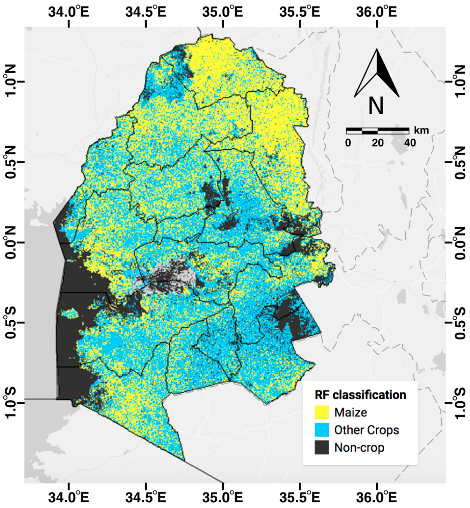
We computed the Sentinel-2 input features using an annual metrics-based compositing approach [16]. Metrics composites are generated by sorting all observations available for a given pixel and extracting the one corresponding to the desired percentile of their distribution. This process is done on a per-band basis, and it is repeated for a prescribed number of percentiles. In this project, we computed the 10th, 25th, 50th, 75th, and 100th percentile of all reflective bands along with their corresponding day-of-year, and the Normalized Difference Vegetation Index (NDVI) and Green Chlorophyll Vegetation Index (GCVI). The metrics-based compositing technique has been already successfully used in several classification studies (e.g., [17]) and has the main advantage of characterizing the target’s phenology implicitly without requiring any assumption on the seasonality. While this configuration was not accurate enough to resolve all different crop types included in the crop cuts, we obtained a test accuracy of 80% after combining the samples in three broader classes: (1) maize crops (MC), (2) other crops (OC), and (3) non-crop (NC). In this final configuration, the random forest classifier was set to use 300 trees, with a minimum leaf sample size of five. The classification map generated using the GEE for the 1AF region is given in Figure 2.
2.4. Satellite Based Yield Estimation
We tested two approaches to estimate yield using satellite images. The first approach, referred to as the “calibrated” approach, related VIs to yield measurements with a simple linear regression model:
where indicates a specific field or administration unit, is the satellite observing date, is the number of image dates, is the weather variable, and ε is the residual error. Here, we used the mean temperature () from May through July; precipitation and vapor pressure deficit were not significant at both the B-K sub-region and the 1AF region based on our preliminary analysis, thus, were excluded from the model. The second approach, referred to as the “uncalibrated” approach, used a well-validated crop model to generate pseudo-observations of yields and VIs to derive the regression coefficients of β in Equations (1) [6,7]. In this way, ground-measured yield was no longer required for calibration. Weather data for the “calibrated” approach and crop simulations were from aWhere database, while MODIS temperature data were used for the 1AF regional yield estimation.
2.4.1. Agricultural Production Systems Simulator (APSIM) Simulation
The Agricultural Production Systems Simulator (APSIM)-Maize model was used to generate 50 simulations for each hypothetical site using a typical range of local sowing dates (Figure S4), initial soil moisture (i.e., 60%, 80%, and 100% of the total extractable soil water), fertilizer rates (i.e., 0, 25, and 50 kg/ha N), and seeding rates (i.e., 3, 4, and 5 plants/m2). The simulated canopy nitrogen content was then converted to daily VIs (e.g., GCVI) based on relationships obtained in field experiments [18] and along with simulated yields were used to build the predictive linear regression model. We used a single cultivar Hybred511, which gives the typical maize phenology in this region, and a single predefined soil profile for the Katumani, Kenya, research station within APSIM for all simulations. Further varying the cultivar maturity length and soil profile properties had nominal impact on yield estimation. Weather inputs to the APSIM model, including daily maximum and minimum temperature, precipitation, and solar radiation, were obtained from the aWhere weather database. We randomly selected two hypothetical sites (i.e., 0.418°N, 34.768°E and 0.682°N, 34.801°E) to generate APSIM simulations for the B-K sub-region, and another seven sites for the 1AF region (Figure 1).
2.4.2 Multiple Avenues to Improve Performance
One underpinning assumption of the uncalibrated approach is that APSIM can reasonably reproduce the seasonal progress of canopy N and yield. However, this assumption can often be violated as shown in several maize model intercomparison studies (e.g., [19,20]). Following our experience with tuning APSIM simulations for rainfed maize in the US Midwest [8], we tested multiple modifications throughout the simulation pipeline.
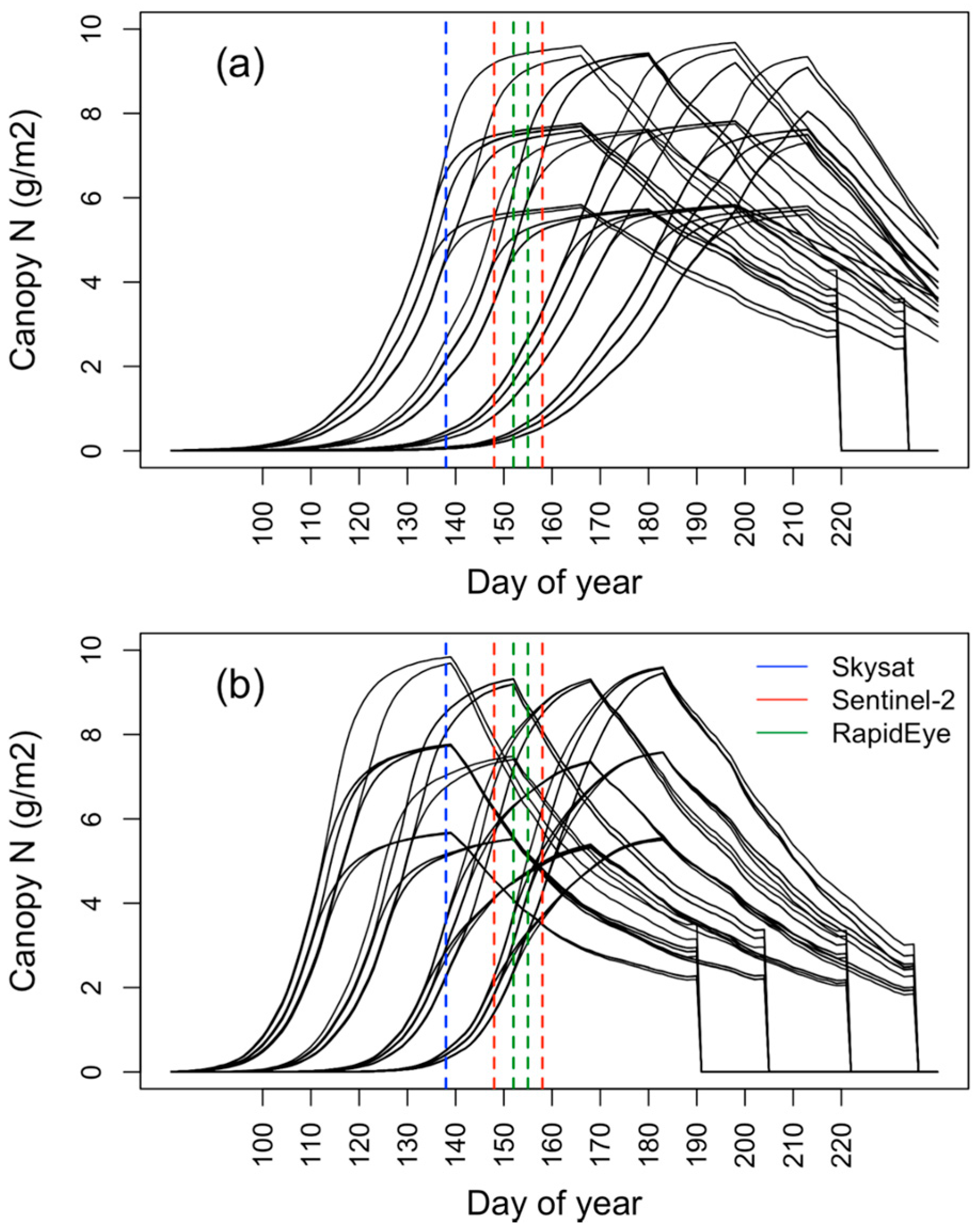
First, we changed a few phenology parameters that control the leaf appearance and senescence to the calibrated values in [8], because simulated canopy green-up curves by the default APSIM phenology parameters were known to be too slow in the early season for modern cultivars [21]. We did not repeat the phenology calibration procedure introduced by reference [8], because it requires frequent cloud-free observations during the growing season thus currently not feasible for the study area. An example of seasonal progress of canopy N (CN) from 50 random simulations of the APSIM-Maize model with default and updated phenology parameters is given in Figure 3. Using the updated phenology advanced the green-up phase and led to more realistic flowering time by early July in 2016.
Second, we compared the difference of using GCVI and MTCI, both of which showed superior performance compared to other VIs in our preliminary analysis, for constructing the linear regression. Following [18], the relationship between GCVI and CN content is:
GCVI = 0.8 × CN
By synthesizing the relationship between MTCI and canopy chlorophyll content (R2 = 0.89) from [21] and the relationship between canopy chlorophyll content and CN (R2 = 0.94) from [18], we converted CN to MTCI using:
MTCI = 0.789 × CN + 3.05
It should also be noted that MTCI from Sentinel-2 has a 20-m resolution, since the Red-edge band of Sentinel-2 has a coarser resolution than that of the NIR or visible bands (Table 1).
Third, existing crop modeling literature (e.g., [22]) suggested that mechanistic simulations of yields by grain formation and growth often underperform simpler approaches that predict yield by multiplying simulated biomass by a constant harvest index (HI). We therefore tested two types of simulations for calibration, one that uses APSIM to directly simulate yields, and another that first uses APSIM to calculate the end-of-season harvestable biomass and then estimates yields by multiplying a constant HI (0.45 in this study). The uncertainty associated with this approach is discussed in details later.
Finally, we tested the effect of using wide vs. narrow sowing windows when generating the representative simulations for each site. Although farmer-reported sowing dates had a wide range from March to May, the majority were within a relative narrower range of about three weeks (Figure S4). Thus, greater weight should be given to simulations from the narrower window. Based on the distribution of 1AF reported sowing dates, we used “15 March”, “25 March”, “8 April”, and “20 April” as the wide sowing window and “1 April”, “5 April”, and “11 April” as the narrow sowing window for the B-K sub-region; for the 1AF region, the wide window was “10 March”, “25 March”, “5 April”, and “15 April”, and the narrow window was “25 March”, “5 April”, and “12 April”.
3. Results
3.1. 1AF-Measured Yield
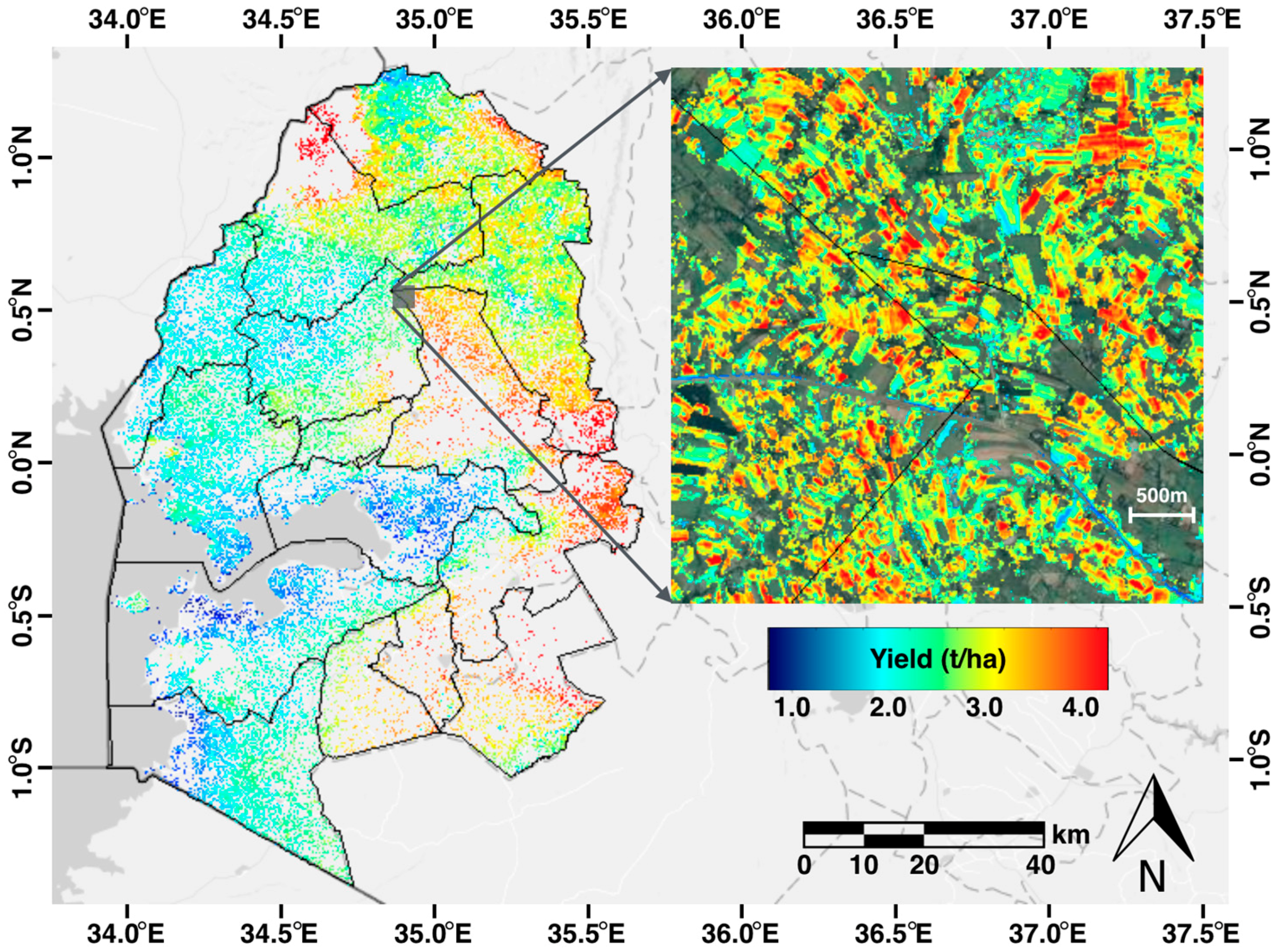
The spatial pattern of crop cut yields in general followed the weather gradient across the study area (Figure 1). Higher yields occurred in the northeast and the southeastern districts, where growing season temperature () was lower and precipitation was abundant (Figure 1e,f). Low yields were mostly reported in the west, where is high. For both districts and divisions, the standard error of the mean for aggregated yields ranged from 100 to over 500 kg/ha (Figure S3). High yield standard errors (greater than 300 kg/ha) located in the north were typically because of a small number of observations. Districts and divisions with lower standard error mostly occurred in the west and the central regions. Reported yields at division level had a higher frequency of yield standard error above 300 kg/ha than at District level, suggesting lower credibility of conclusions made at the division level.
3.2. Performance of Multiple VIs at Bungoma
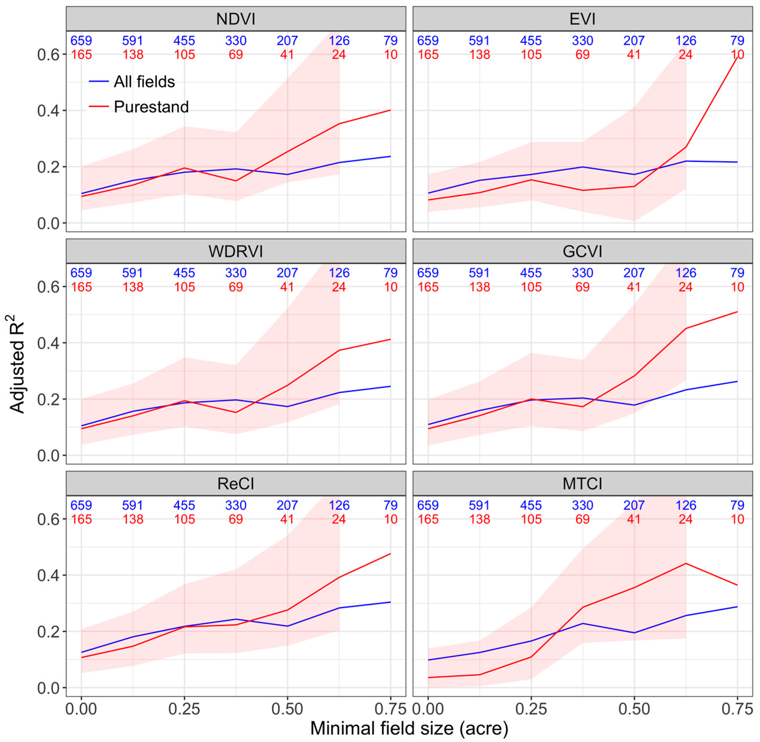
For all VIs tested, the agreement (as measured by adjusted R2) between ground-measured and satellite-derived calibrated yield estimates was consistently better on larger fields, especially when field size was greater than 0.5 acre (Figure 4). Almost all VIs tested can explain more than 40% of the variation in measured yields when field size was greater than 0.75 acre, although the value should be interpreted with caution because the sample size was small (i.e., 10 fields). Not surprisingly, purestand fields outperformed estimates for intercropped fields when field size was greater than 0.5 acre. However, purestand fields only account for about 20% of the total surveyed fields (Figure 4). Both GCVI and MTCI outperformed other indices (although differences were not statistically significant due to small sample sizes) for fields between 0.5 and 0.75 acre, among which MTCI captured about 35% and 45% of the yield variation when minimal field size was 0.5 and 0.625 acre, respectively. We therefore selected GCVI and MTCI for further yield estimation on a regional scale, and designated the regression model for purestand fields with minimal size of 0.5 acre as the preferred calibrated model for the B-K sub-region (Table S1). Among the independent variables, both the Skysat imagery on 17 May and the RapidEye imagery on 1 June and 4 June contributed to the model performance as the adjusted R2 was lower when either of them were removed from the regression. The usefulness of the early season Skysat imagery was likely because it helped capture differences in sowing dates.
3.3. Performance of the Calibrated Model
The preferred calibrated model for the B-K sub-region explained 28.2% and 35.6% of yield variations in purestand fields when using GCVI and MTCI as explanatory variables, respectively (Table 3). Such performances were competitive to the model proposed by [7] for the similar region, which purely used cloud-free Skysat imagery as explanatory variables. The remaining unexplained variation in yields can be attributed to other factors such as the presence of weeds and the fraction of the planted area that was not harvested (typically due to drought, waterlogging, animal damage, or theft). However, these factors were not quantitatively surveyed and thus could not be assessed directly.
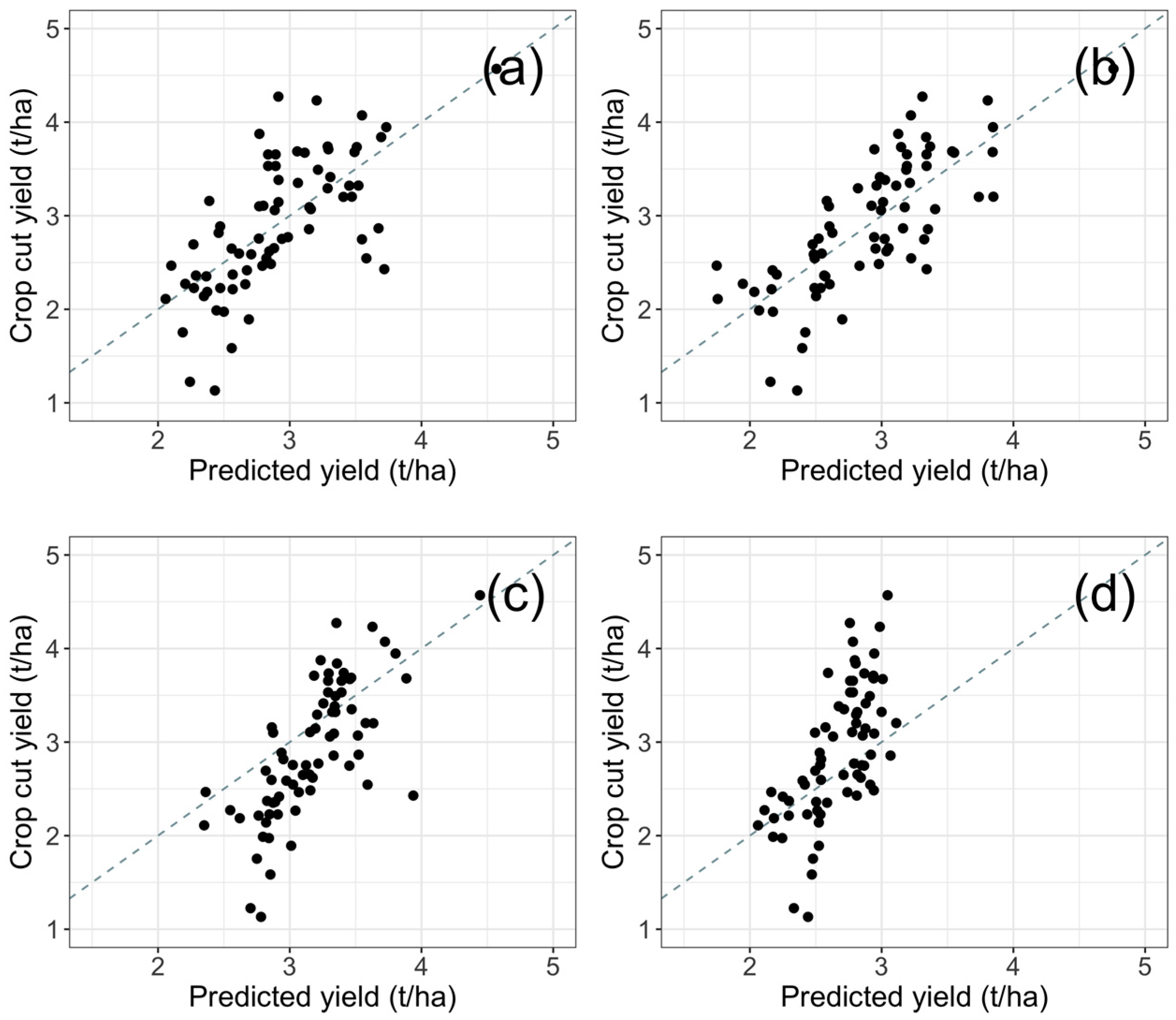
The calibrated model for the 1AF Region that used Tavg and the coarser resolution Sentinel-2 imagery as the explanatory variables had fairly good performance, especially at the district level where aggregated yield measurements were most reliable (Table 3; Figure 5a,b). Using MTCI instead of GCVI improved the model adjusted R2 by 25% at the division level and 31% at the district level, although MTCI data were only half of the spatial resolution as that of the GCVI data due to the coarser resolution of red edge bands of Sentinel-2 (Table 1). Excluding districts from the “Kisii” and “Nyamira” County in the south that had either much earlier or wider range of sowing dates further improved calibrated models (Table 3). Yield estimates were mostly between 2 to 4 t/ha and were slightly smaller than the measurement range of 1 to 4 t/ha (Figure 5a,b). The best performance was achieved when using MTCI at the district level, which captured 57% and 66% of the crop cut yield variations with and without the two early sowing counties, respectively. This level of agreement between predicted and measured yields was close to [23], who trained a multiple regression model for southwestern Kenya with a range of satellite and ground-level data such as NDVI, agrometeorological data, and government produced maps of crop yields and area planted.
3.4. Performance of the Uncalibrated Model
The uncalibrated model coefficients and associated R2 of the regressions derived from APSIM-Maize simulations for both the B-K sub-region and the 1AF region are listed in Tables S1 and S2. In general, using updated phenology parameters and a narrower sowing window significantly improved the R2 of the regression using simulated data. (Using GCVI vs. MTCI had no effect on the calibration R2 because conversions between CN and VIs were all linear.) In the B-K sub-region, the uncalibrated yield estimates, derived by applying these coefficients to the actual observations of GCVI or MTCI, were slightly worse than the calibrated model estimates (Table 4), but still captured up to one-third of the variation for purestand fields with minimal size of 0.5 acre. The agreement between measured yields and uncalibrated model estimates was highest for the model built on simulations with updated phenology parameters, MTCI, Biomass×HI estimation, and narrow sowing window. Prediction performance was mostly unsatisfying for the full survey sample (including very small and intercropped fields), except for cases when updated phenology parameter and narrow sowing window were used.
For the broader 1AF region, uncalibrated model estimates were fairly encouraging, capturing about one-third of the ground-based yield variations at the division level, and nearly half of variability at the district level (Table 4). The overall better performance at the district level was likely in part due to smaller standard error in the crop cut yields aggregation (Figure S3). Overall, models derived from pseudo training samples with MTCI and Biomass×HI estimation had better performance, and were not affected by the width of sowing window. Surprisingly, although models derived from default phenology per se had smaller R2 for training on simulations than that of models using updated phenology (Table S2), the former actually did a better job than the latter in yield estimation as measured by the adjusted R2 (Table 4) and the spread of estimates (Figure 5c,d). We believe this was likely because the larger regression coefficient for in models with default phenology better captured the spatial gradient in temperature, which was a significant explanatory variable for yields in the 2016 growing season.
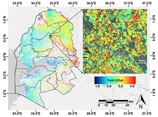
A map of the yield estimates for the 1AF region using the uncalibrated model derived from APSIM simulations with default phenology, MTCI, Biomass×HI estimation, and Narrow sowing window is given in Figure 6. The spatial pattern of low-high yields matched well with the 1AF measurements (Figure 1c) and a high spatial correlation with can be distinguished (Figure 1e). Importantly, the satellite estimates capture both these broad gradients as well as large amounts of yield variation at finer spatial scales within and between fields (Figure 6).
4. Discussion
Our results highlight the potential of using high-resolution satellite imagery for generating smallholder productivity estimates. Overall, by using two or three relatively cloud-free satellite images and growing season mean temperature, we successfully capture about one-third to one-half of the variation in yield measurements. The competitive performance by the uncalibrated approach is noteworthy as this approach does not require any ground data for calibration and, thus, has a greater potential for scale up to broader regions. Although a considerable amount of variability in ground-based yield estimates remains unexplained by our satellite estimates, some of this variability is likely noise in the ground-based estimates, as indicated by the fact that results were better when using district than division aggregates. Moreover, satellite-based estimates do not need to be perfect to be useful for a range of applications [4]. For example, yield differences can be used to evaluate the impact of certain agricultural interventions by governmental programs or nongovernmental organization (NGO) projects. Furthermore, the ability to map yield at field level across a region over time could contribute to our ability to understand the magnitude and determinants of yield gaps, thus enabling more effective transformation in agronomic managements.
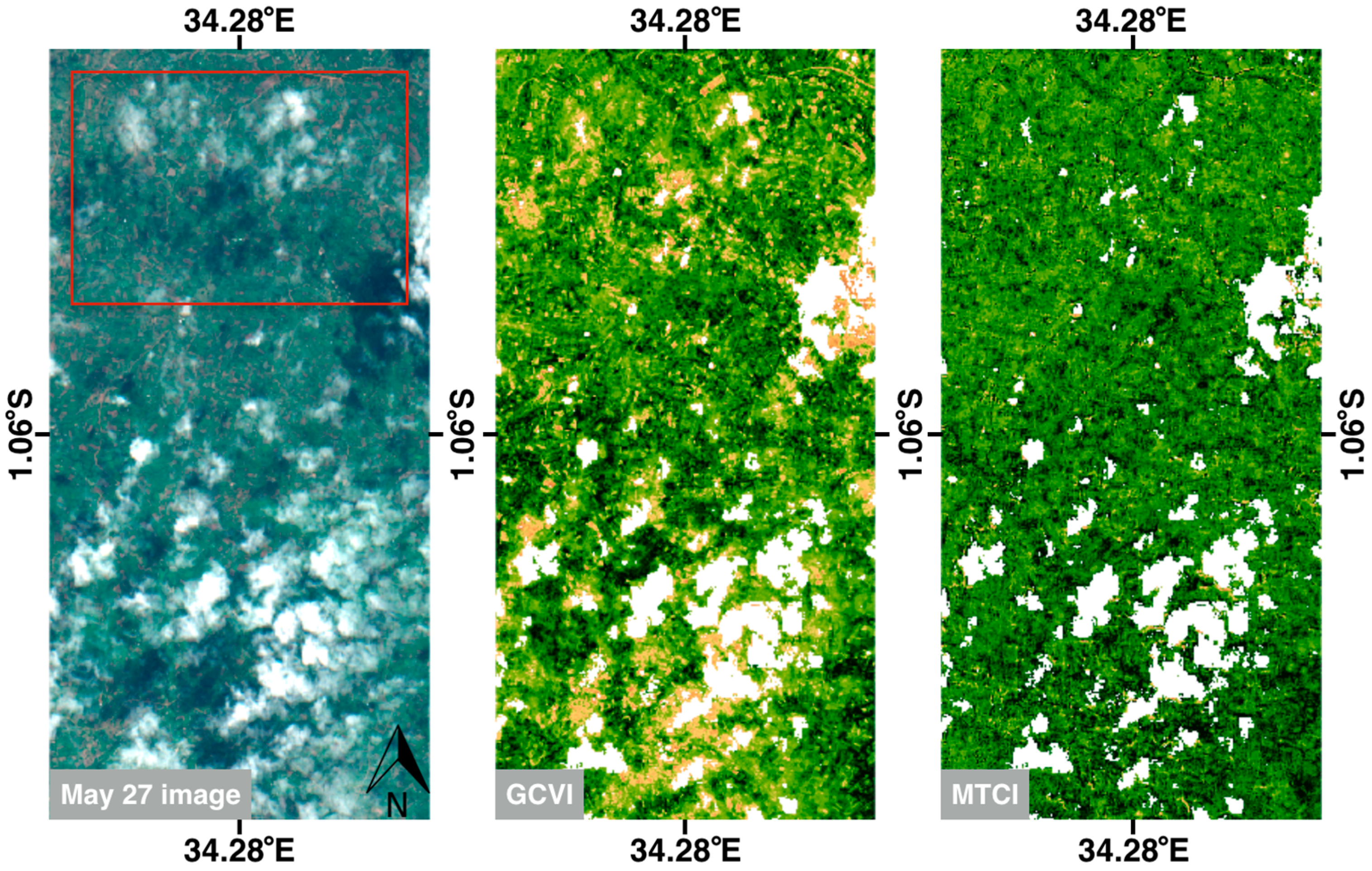
Several of the multiple refinements tested in this study helped to improve the uncalibrated model performance, among which using MTCI seems to be the most effective option in this region. The consistent outperformance of MTCI compared to other VIs for both the B-K sub-region and the 1AF region is likely due in part to its greater sensitivity to canopy chlorophyll content [15,24]. Potentially more important is the fact that MTCI is much less affected by atmospheric conditions because its calculation is based on the difference in reflectance between two nearby bands that will be similarly affected by atmospheric scattering [15]. As is highlighted in Figure 7, GCVI showed obvious patterns associated with cloud edges and haze, whereas MTCI was less affected. Unfortunately, several of the most recent high-resolution satellite sensors (e.g., Planet Scope and Worldview series) lack the red edge bands for calculating MTCI.
A second lesson, consistent with the study of the US by reference [8], is that using Biomass×HI to derive yields for training was consistently superior to relying on the direct APSIM yield simulation. The poorer performance by using APSIM simulated yields instead of biomass likely indicates the weaker capability of APSIM in reproducing the temperature effect on grain number and grain filling rate (which jointly determined the end-season yield) than the effect on photosynthesis and biomass accumulation; thus, the more mechanistic simulation of grain number and grain filling adds another layer of uncertainty. Using constant HI works well likely because a substantial fraction of weather-induced HI variability is already captured by the biomass by the time when total kernel numbers is determined (i.e., flowering stage in APSIM), thus, a dynamic HI approach may double-account the weather stress. Employing other crop models is not likely a promising solution, because almost all crop models have no memory of the temperature effects on photosynthesis that will be carried over to yield production [23].
Contrary to our expectation, using updated phenology parameters did not improve the yield estimation, even though the updated parameters resulted in more realistic timing of the peak season. One caveat is that we only tested a set of parameters that were derived in the US Midwest, which may not fit this tropical region. As more frequent imagery has become available since the 2017 growing season, we expect to further improve the uncalibrated approach after conducting a phenology calibration locally as well as deriving a set of APSIM cultivars for this region. Using a narrower sowing window, which considerably increased the R2 of the training regression model, also did not meaningfully improve the yield prediction.
Finally, the current land classification map could be a significant source of uncertainty to our yield estimates on a regional scale. The random forest classifier we used to generate the regional land cover map was originally trained for the B-K sub-region, but has not been tested for the 1AF region due to a lack of ground data. Based on our visual check, the classifier was slightly weak in distinguishing maize field with trees and shrubs. Our future plan is to collect more ground information on field crop type across the 1AF region through our local partners.
5. Conclusions
This study showed that multiple high-resolution satellite sensors can be used to derive models for predicting yields of smallholder farms. The calibrated models that were trained using ground data roughly captured one-third of the variation in surveyed yields, and more than one-half at aggregated administrative units. An alternative scalable uncalibrated approach that did not require yield measurements for calibration performed almost as well as the calibrated approach, especially at the aggregated units. The proposed preferred model successfully captured the spatial pattern of yield gradient at a regional scale, and highlighted the within- and between-field yield heterogeneity at a local scale. We also tested multiple approaches in this study to improve the uncalibrated model performance, among which using MTCI instead of GCVI and using a fixed ratio of yield to biomass had consistent benefits in this region. Further improvement can be expected in the near future when more frequent satellite observations throughout the growing season become available (e.g., from Sentinel-2 and Planet constellations). Overall, yield mapping in this region is very challenging due to the considerable landscape heterogeneity, small field sizes, and prevalence of intercropping. Yet our results suggest that the recently available satellite missions are a viable tool to estimate and understand yield variation at the field scale across smallholder farms in Africa, and the methodology presented in this study could serve as a good foundation for other smallholder farming systems in the world.
Supplementary Materials
The following are available online at www.mdpi.com/2072-4292/9/9/931/s1.
Acknowledgments
We acknowledge Ben Wekesa and Peter LeFrancois for leading field survey data collection in Bungoma. We thank One Acre Fund for leading the crop cut measurements and in particular Kalie Gold and Charles Ogechi for coordinating the data collection. We also thank Planet for providing the RapidEye imagery and Terra Bella for providing the Skysat imagery. Partial support for this project was provided by the Feed the Future Innovation Lab for Sustainable Intensification (Cooperative Agreement No. AID-OAA-L-14-00006), funded by the United States Agency for International Development (USAID). The contents are the sole responsibility of the authors and do not necessarily reflect the views of USAID or the United States Government.
Author Contributions
Zhenong Jin, Marshall Burke, and David Lobell conceived of the work. All authors collected and processed the data. Zhenong Jin and David Lobell wrote the first draft of the manuscript, and all authors contributed to the final manuscript.
Conflicts of Interest
The authors declare no conflict of interest.
References
- World Bank World Development Report 2008—Agriculture for Development. Available online: https://openknowledge.worldbank.org/handle/10986/5990 (accessed on 5 September 2017).
- Morton, J.F. The impact of climate change on smallholder and subsistence agriculture. Proc. Natl. Acad. Sci. USA 2007, 104, 19680–19685. [Google Scholar] [CrossRef] [PubMed]
- Carletto, C.; Jolliffe, D.; Banerjee, R. From Tragedy to Renaissance: Improving Agricultural Data for Better Policies. J. Dev. Stud. 2015, 51, 133–148. [Google Scholar] [CrossRef]
- Lobell, D.B. The use of satellite data for crop yield gap analysis. Field Crop. Res. 2013, 143, 56–64. [Google Scholar] [CrossRef]
- Shelestov, A.; Lavreniuk, M.; Kussul, N.; Novikov, A.; Skakun, S. Exploring Google Earth Engine Platform for Big Data Processing: Classification of Multi-Temporal Satellite Imagery for Crop Mapping. Front. Earth Sci. 2017, 5, 1–10. [Google Scholar] [CrossRef]
- Lobell, D.B.; Thau, D.; Seifert, C.; Engle, E.; Little, B. A scalable satellite-based crop yield mapper. Remote Sens. Environ. 2015, 164, 324–333. [Google Scholar] [CrossRef]
- Burke, M.; Lobell, D.B. Satellite-based assessment of yield variation and its determinants in smallholder African systems. Proc. Natl. Acad. Sci. USA 2017, 114, 2189–2194. [Google Scholar] [CrossRef] [PubMed]
- Jin, Z.; Azzari, G.; Lobell, D.B. Improving the accuracy of satellite-based high-resolution yield estimation: A test of multiple scalable approaches. Agric. For. Meteorol. 2017, 247, 207–220. [Google Scholar]
- Carletto, C.; Gourlay, S.; Winters, P. From guesstimates to GPStimates: Land area measurement and implications for agricultural analysis. J. Afr. Econ. 2015, 24, 593–628. [Google Scholar] [CrossRef]
- Vancutsem, C.; Ceccato, P.; Dinku, T.; Connor, S.J. Evaluation of MODIS land surface temperature data to estimate air temperature in different ecosystems over Africa. Remote Sens. Environ. 2010, 114, 449–465. [Google Scholar] [CrossRef]
- Rouse, J.W.; Haas, R.H.; Schell, J.A.; Deering, D.W. Monitoring Vegetation Systems in the Great Okains with ERTS. In Proceedings of the Third Earth Resources Technology Satellite-1 Symposium, Washington, DC, USA, 10–14 December 1973; Freden, S.C., Mercanti, E.P., Eds.; NASA: Washington, DC, USA, 1974. [Google Scholar]
- Huete, A.R.; Liu, H.Q.; Batchily, K.; Van Leeuwen, W. A comparison of vegetation indices over a global set of TM images for EOS-MODIS. Remote Sens. Environ. 1997, 59, 440–451. [Google Scholar] [CrossRef]
- Gitelson, A.A. Wide Dynamic Range Vegetation Index for remote quantification of biophysical characteristics of vegetation. J. Plant Physiol. 2004, 161, 165–173. [Google Scholar] [CrossRef] [PubMed]
- Gitelson, A.A.; Gritz, Y.; Merzlyak, M.N. Relationships between leaf chlorophyll content and spectral reflectance and algorithms for non-destructive chlorophyll assessment in higher plant leaves. J. Plant Physiol. 2003, 160, 271–282. [Google Scholar] [CrossRef] [PubMed]
- Dash, J.; Curran, P.J. The MERIS terrestrial chlorophyll index. Int. J. Remote Sens. 2004, 2523, 5403–5413. [Google Scholar] [CrossRef]
- Hansen, M.C.; Egorov, A.; Potapov, P.V.; Stehman, S.V.; Tyukavina, A.; Turubanova, S.A.; Roy, D.P.; Goetz, S.J.; Loveland, T.R.; Ju, J.; et al. Monitoring conterminous United States (CONUS) land cover change with Web-Enabled Landsat Data (WELD). Remote Sens. Environ. 2014, 140, 466–484. [Google Scholar] [CrossRef]
- Azzari, G.; Lobell, D.B. Landsat-based classification in the cloud: An opportunity for a paradigm shift in land cover monitoring. Remote Sens. Environ. 2017. [Google Scholar] [CrossRef]
- Schlemmera, M.; Gitelson, A.; Schepersa, J.; Fergusona, R.; Peng, Y.; Shanahana, J.; Rundquist, D. Remote estimation of nitrogen and chlorophyll contents in maize at leaf and canopy levels. Int. J. Appl. Earth Obs. Geoinf. 2013, 25, 47–54. [Google Scholar] [CrossRef]
- Bassu, S.; Brisson, N.; Durand, J.-L.L.; Boote, K.; Lizaso, J.; Jones, J.W.; Rosenzweig, C.; Ruane, A.C.; Adam, M.; Baron, C.; et al. How do various maize crop models vary in their responses to climate change factors? Glob. Chang. Biol. 2014, 20, 2301–2320. [Google Scholar] [CrossRef] [PubMed]
- Kumudini, S.; Andrade, F.H.; Boote, K.J.; Brown, G.A.; Dzotsi, K.A.; Edmeades, G.O.; Gocken, T.; Goodwin, M.; Halter, A.L.; Hammer, G.L.; et al. Predicting maize phenology: Intercomparison of functions for developmental response to temperature. Agron. J. 2014, 106, 2087–2097. [Google Scholar] [CrossRef]
- Archontoulis, S.V.; Miguez, F.E.; Moore, K.J. Evaluating APSIM Maize, Soil Water, Soil Nitrogen, Manure, and Soil Temperature Modules in the Midwestern United States. Agron. J. 2014, 106, 1025. [Google Scholar] [CrossRef]
- Jin, Z.; Zhuang, Q.; Tan, Z.; Dukes, J.S.; Zheng, B.; Melillo, J.M. Do maize models capture the impacts of heat and drought stresses on yield? Using algorithm ensembles to identify successful approaches. Glob. Chang. Biol. 2016, 22, 3112–3126. [Google Scholar] [CrossRef] [PubMed]
- Rojas, O. Operational maize yield model development and validation based on remote sensing and agro-meteorological data in Kenya. Int. J. Remote Sens. 2007, 28, 3775–3793. [Google Scholar] [CrossRef]
- Peng, Y.; Nguy-Robertson, A.; Arkebauer, T.; Gitelson, A.A. Assessment of canopy chlorophyll content retrieval in maize and soybean: Implications of hysteresis on the development of generic algorithms. Remote Sens. 2017, 9, 226. [Google Scholar] [CrossRef]
Figure 1.
Study region in west Kenya (a). Grey area is where One Acre Fund crop cut yields are available; (b) individual crop cut yields (black boundaries delineate counties and grey boundaries delineate districts); and (c) aggregated crop cut yields at District level with star symbols showing the hypothetical sites for crop model simulations. (d) Sub-region from where household survey data come. (e) Apr-July mean temperature; and (f) total precipitation in 2016 is given with the colored rectangle indicating the surveyed sub-region.

Figure 2.
Land cover classification of the study area. Map was generated using Sentinel-2 imagery with a spatial resolution of 10 m.
Figure 2.
Land cover classification of the study area. Map was generated using Sentinel-2 imagery with a spatial resolution of 10 m.

Figure 3.
An example of seasonal progress in canopy nitrogen from 50 random simulations by the Agricultural Production Systems Simulator (APSIM)-Maize model with default (a) and updated (b) phenology parameters (e.g., leaf appearance and senescence). The clustering of simulated curves over the day of year reflects four different sowing dates used in the simulation (i.e., “15 March”, “25 March”, “8 April”, and “20 April”). The timing when cloud-free satellite imagery was available is highlighted in colored vertical lines.

Figure 4.
Performance of VIs in predicting farmer-reported yields as a function of field size for 2016. Numbers at the top of each panel show the number of fields included in each estimate. Red shaded region reports bootstrapped 95% confidence interval on the purestand-field estimates.
Figure 4.
Performance of VIs in predicting farmer-reported yields as a function of field size for 2016. Numbers at the top of each panel show the number of fields included in each estimate. Red shaded region reports bootstrapped 95% confidence interval on the purestand-field estimates.

Figure 5.
Comparison of selected model predictions with crop cut yields. (a) Calibrated model with GCVI, (b) calibrated model with MTCI, (c) uncalibrated model with default phenology parameter and MTCI, and (d) uncalibrated model with updated phenology parameter and MTCI. Grey dashed lines indicate 1:1 line.

Figure 6.
An example of yield estimates for the 1AF region in 2016 using the uncalibrated model and Sentinel-2 data. The inset panel is an example of finer scale yield estimates.
Figure 6.
An example of yield estimates for the 1AF region in 2016 using the uncalibrated model and Sentinel-2 data. The inset panel is an example of finer scale yield estimates.

Figure 7.
Snapshots of June 7 image by Sentinel-2 in raw and the derived GCVI and MTCI. A red square highlighted the area where cloud contamination affected the GCVI more than MTCI.
Figure 7.
Snapshots of June 7 image by Sentinel-2 in raw and the derived GCVI and MTCI. A red square highlighted the area where cloud contamination affected the GCVI more than MTCI.


Table 1.
Spectral information of multiple sensors used in this study.
| Band | Use | Spectral Range | Pixel Size |
|---|---|---|---|
| Skysat | |||
| B | Blue | 450–515 nm | 2 m |
| G | Green | 515–595 nm | 2 m |
| R | Red | 605–695 nm | 2 m |
| N | Near Infrared (NIR) | 740–900 nm | 2 m |
| RapidEye | |||
| b1 | Blue | 440–510 nm | 5 m |
| b2 | Green | 520–590 nm | 5 m |
| b3 | Red | 630–685 nm | 5 m |
| b4 | Red Edge (RE) | 690–730 nm | 5 m |
| b5 | NIR | 760–850 nm | 5 m |
| Sentinel-2 | |||
| B2 | Blue | 458–523 nm | 10 m |
| B3 | Green | 543–578 nm | 10 m |
| B4 | Red | 650–680 nm | 10 m |
| B5 | Red Edge (RE) | 698–713 nm | 20 m |
| B8 | NIR | 785–900 nm | 10 m |
Table 2.
Vegetation indices (VIs) tested in this study. Bands used to calculate these VIs were defined in Table 1.
Table 2.
Vegetation indices (VIs) tested in this study. Bands used to calculate these VIs were defined in Table 1.
| Vegetation Index | Formula | Reference |
|---|---|---|
| Normalized Difference Vegetation Index (NDVI) | (NIR − Red)/(NIR + Red) | Rouse et al., 1973 [11] |
| Enhanced Vegetation Index (EVI) | 2.5 × (NIR − Red)/(NIR + 6 × Red + 7 × Blue − 1) | Huete et al., 1997 [12] |
| Wide Dynamic Range Vegetation Index (WDRVI) | (0.2 × NIR − Red)/(0.2 × NIR + Red) | Gitelson, 2004 [13] |
| Green Chlorophyll Vegetation Index (GCVI) | (NIR/Green − 1) | Gitelson et al., 2003 [14] |
| Red edge Chlorophyll Index (ReCI) | NIR/RE − 1 | Gitelson et al., 2003 [14] |
| MERIS Terrestrial Chlorophyll Index (MTCI) | (NIR − RE)/(RE − Red) | Dash and Curran, 2004 [15] |
Table 3.
Adjusted coefficient of determination (R2) of calibrated regression model that was trained using ground yield data. Values for the B-K sub-region (Bungoma and Kakamega counties) were derived from regressions with fields larger than 0.5 acre. Values in the brackets were derived from regression that excluded two counties with early sowing. Values within each column or each row were not statistically different based on F-tests. 1AF = One Acre Fund.
| Vegetation Index | B-K Sub-region | 1AF Region | ||
|---|---|---|---|---|
| Full | Purestand | Division | District | |
| GCVI | 0.18 | 0.28 | 0.29 (0.36) | 0.43 (0.49) |
| MTCI | 0.20 | 0.36 | 0.36 (0.44) | 0.57 (0.66) |
Table 4.
Adjusted coefficient of determination (R2) of uncalibrated regression model that was trained using crop model simulations. HI = harvest index.
Table 4.
Adjusted coefficient of determination (R2) of uncalibrated regression model that was trained using crop model simulations. HI = harvest index.
| Simulation Settings | B-K Sub-region | 1AF Region | |||||
|---|---|---|---|---|---|---|---|
| Phenology | VI | Yield Estimates | Sowing Window | Full | Purestand | Division | District |
| Default | GCVI | Yields | Wide | 0.018 | 0.038 | 0.277 ** | 0.426 ** |
| Default | GCVI | Yields | Narrow | 0.009 | 0 | 0..279 ** | 0.424 ** |
| Default | GCVI | Biomass×HI | Wide | 0.007 | 0.02 | 0.285 ** | 0.423 ** |
| Default | GCVI | Biomass×HI | Narrow | 0 | 0 | 0.281 ** | 0.42 ** |
| Default | MTCI | Yields | Wide | 0.016 | 0.238 ** | 0.335 ** | 0.525 ** |
| Default | MTCI | Yields | Narrow | 0.013 | 0.208 * | 0.349 ** | 0.531 ** |
| Default | MTCI | Biomass×HI | Wide | 0.007 | 0.204 * | 0.355 ** | 0.51 ** |
| Default | MTCI | Biomass×HI | Narrow | 0 | 0.118 ˙ | 0.349 ** | 0.509 ** |
| Updated | GCVI | Yields | Wide | 0.015 | 0 | 0.116 ** | 0.112 ** |
| Updated | GCVI | Yields | Narrow | 0.11 ˙ | 0.25 ** | 0.21 ** | 0.291 ** |
| Updated | GCVI | Biomass×HI | Wide | 0 | 0 | 0.284 ** | 0.413 ** |
| Updated | GCVI | Biomass×HI | Narrow | 0.172* | 0.169* | 0.289 ** | 0.421 ** |
| Updated | MTCI | Yields | Wide | 0.006 | 0.115 ˙ | 0.109 ** | 0.116 ** |
| Updated | MTCI | Yields | Narrow | 0.06 | 0.222 ** | 0.19 ** | 0.255 ** |
| Updated | MTCI | Biomass×HI | Wide | 0 | 0.102 ˙ | 0.293 ** | 0.404 ** |
| Updated | MTCI | Biomass×HI | Narrow | 0.147 * | 0.363 ** | 0.316 ** | 0.44 ** |
Note: Significance level: ** for p-value < 0.001, * for p-value < 0.01, ˙ for p-value < 0.05.
© 2017 by the authors. Licensee MDPI, Basel, Switzerland. This article is an open access article distributed under the terms and conditions of the Creative Commons Attribution (CC BY) license (http://creativecommons.org/licenses/by/4.0/).
Share and Cite
MDPI and ACS Style
Jin, Z.; Azzari, G.; Burke, M.; Aston, S.; Lobell, D.B. Mapping Smallholder Yield Heterogeneity at Multiple Scales in Eastern Africa. Remote Sens. 2017, 9, 931. https://0-doi-org.brum.beds.ac.uk/10.3390/rs9090931
AMA Style
Jin Z, Azzari G, Burke M, Aston S, Lobell DB. Mapping Smallholder Yield Heterogeneity at Multiple Scales in Eastern Africa. Remote Sensing. 2017; 9(9):931. https://0-doi-org.brum.beds.ac.uk/10.3390/rs9090931
Chicago/Turabian StyleJin, Zhenong, George Azzari, Marshall Burke, Stephen Aston, and David B. Lobell. 2017. "Mapping Smallholder Yield Heterogeneity at Multiple Scales in Eastern Africa" Remote Sensing 9, no. 9: 931. https://0-doi-org.brum.beds.ac.uk/10.3390/rs9090931
Note that from the first issue of 2016, this journal uses article numbers instead of page numbers. See further details here.