Evaluation of Remote-Sensing-Based Landslide Inventories for Hazard Assessment in Southern Kyrgyzstan

Abstract

Large areas in southern Kyrgyzstan are subjected to high and ongoing landslide activity; however, an objective and systematic assessment of landslide susceptibility at a regional level has not yet been conducted. In this paper, we investigate the contribution that remote sensing can provide to facilitate a quantitative landslide hazard assessment at a regional scale under the condition of data scarcity. We performed a landslide susceptibility and hazard assessment based on a multi-temporal landslide inventory that was derived from a 30-year time series of satellite remote sensing data using an automated identification approach. To evaluate the effect of the resulting inventory on the landslide susceptibility assessment, we calculated an alternative susceptibility model using a historical inventory that was derived by an expert through combining visual interpretation of remote sensing data with already existing knowledge on landslide activity in this region. For both susceptibility models, the same predisposing factors were used: geology, stream power index, absolute height, aspect and slope. A comparison of the two models revealed that using the multi-temporal landslide inventory covering the 30-year period results in model coefficients and susceptibility values that more strongly reflect the properties of the most recent landslide activity. Overall, both susceptibility maps present the highest susceptibility values for similar regions and are characterized by acceptable to high predictive performances. We conclude that the results of the automated landslide detection provide a suitable landslide inventory for a reliable large-area landslide susceptibility assessment. We also used the temporal information of the automatically detected multi-temporal landslide inventory to assess the temporal component of landslide hazard in the form of exceedance probability. The results show the great potential of satellite remote sensing for deriving detailed and systematic spatio-temporal information on landslide occurrences, which can significantly improve landslide susceptibility and hazard assessment at a regional scale, particularly in data-scarce regions such as Kyrgyzstan.

1. Introduction

The eastern rim of the Fergana Basin in southern Kyrgyzstan is a tectonically active region that experiences regular landslide occurrences. The threat to people and infrastructure posed by this high landslide activity requires a systematic and objective assessment of the landslide hazard, which has not yet been performed for this region. Although analyses of landslide susceptibility have been conducted by local experts, these analyses have been of a qualitative nature and concentrated on areas in the vicinity of settlements and roads. Factors that complicate this task are the large size of the study area (approximately 2300 km²) and the limited availability of spatially detailed and up-to-date information on landslide occurrences and predisposing factors.

In such a setting, the use of satellite remote sensing has high potential for large-area detailed characterization of predisposing factors and for the generation of improved landslide inventories. Using time series of archived remote sensing data enables multi-temporal reconstruction of backdated landslide occurrences for large areas covering a time period of several decades. However, such a task requires analyzing large amounts of remote sensing data, which can only be accomplished using automated methods. We have developed such a method for the automated object-based detection of landslide occurrences using multi-sensor time series of optical satellite images [1,2]. This method is based on the analysis of normalized difference vegetation index (NDVI) trajectories [3] and has been successfully applied in this study area [2]. In this paper, we investigate the suitability of the resulting systematic multi-temporal landslide inventory covering a 30-year time period for conducting subsequent analyses of landslide susceptibility and hazard.

Landslide susceptibility analysis is the first step in the overall framework of landslide hazard and risk assessment [4,5,6,7]. This analysis requires spatial information on past landslide occurrences (landslide inventory) and spatial characterization of landslide predisposing factors to evaluate the spatial probability of where landslides may occur in the future. The reliability of susceptibility mapping is significantly influenced by the quality and completeness of the landslide inventory. To achieve a high degree of completeness, different information sources have to be analyzed, thus resulting in different types of landslide inventories.

Guzzetti et al. [5] distinguish between the following inventory types: archive inventory (based on records in archives, newspapers, and so on), historical inventory (showing the cumulative effect of landsliding over a long period of time without further temporal differentiation), event-based inventory (landslides caused by a single triggering event, such as a strong earthquake), seasonal inventory (landslides triggered within one active season) and multi-temporal inventory (continuous monitoring of landslide activity over longer periods of time independent of particular triggering events). The multi-temporal inventory is the most labor-intensive inventory type and the only one with the potential for spatio-temporal completeness, and it generally requires the use of remote sensing [2].

The majority of the research on landslide hazard focuses on assessing landslide susceptibility, often because of difficulties in obtaining the multi-temporal information on landslide occurrences required for landslide hazard analysis [8]. At the methodological level, many papers compare results obtained using different susceptibility calculation approaches, such as logistic regression, frequency ratio, and neural networks, among others [9,10,11,12]. Since all of these methods are data-driven methods, the resulting models also largely depend on the type and quality of the input data, although this aspect generally receives less attention. However, several publications also discuss the influence of the type and quality of the used landslide inventory information on the results of susceptibility mapping [8,13,14,15].

In our investigation, we focus on the influence of the inventory properties on landslide susceptibility and hazard analysis with special consideration of the contribution of satellite remote sensing. For this purpose, we derived two landslide inventories: (i) a systematic multi-temporal inventory generated by automated landslide detection from time series of satellite remote sensing data and (ii) a historical inventory prepared by an expert based on the visual interpretation of high-resolution satellite remote sensing data as well as incorporating already existing knowledge on landslide occurrences. Detailed descriptions of the methodologies used for the derivation of these two inventories can be found in [1,2,16,17].

The historical inventory represents the more conventional approach to landslide mapping, and it requires the time-consuming involvement of an expert. This inventory allows the cumulative assessment of landslide activity that has occurred in an area up to the time when the inventory is prepared. Since the historical inventory incorporates all available records, the quality of the inventory also depends on the overall availability of historical information for a specific region. Using high-resolution satellite remote sensing can partially compensate for missing historical documentation as long as the morphological indicators for past landslide activity are still present in today’s relief. Historical inventories are generally limited in terms of temporal information on landslide occurrences. However, such information is needed to provide the temporal component required for landslide hazard analysis [5].

Preparing the necessary multi-temporal inventories including multiple time steps—ideally after each triggering event and/or period of landslide activation—imposes limits on manual approaches of landslide mapping, particularly if large areas need to be analyzed. Therefore, remote-sensing-based automated approaches become increasingly more important. In this study, we pose the question of to what extent the use of an automatically derived multi-temporal remote-sensing-based landslide inventory leads to different results in the susceptibility analysis compared to the historical inventory prepared by an expert. Furthermore, we aim to investigate the potential of the multi-temporal nature of the automatically derived inventory for assessing the temporal component of landslide hazard, which to date has received less attention among the scientific contributions toward improved hazard assessment because of the widespread lack of suitable multi-temporal data on landslide occurrences.

2. Study Area and Database

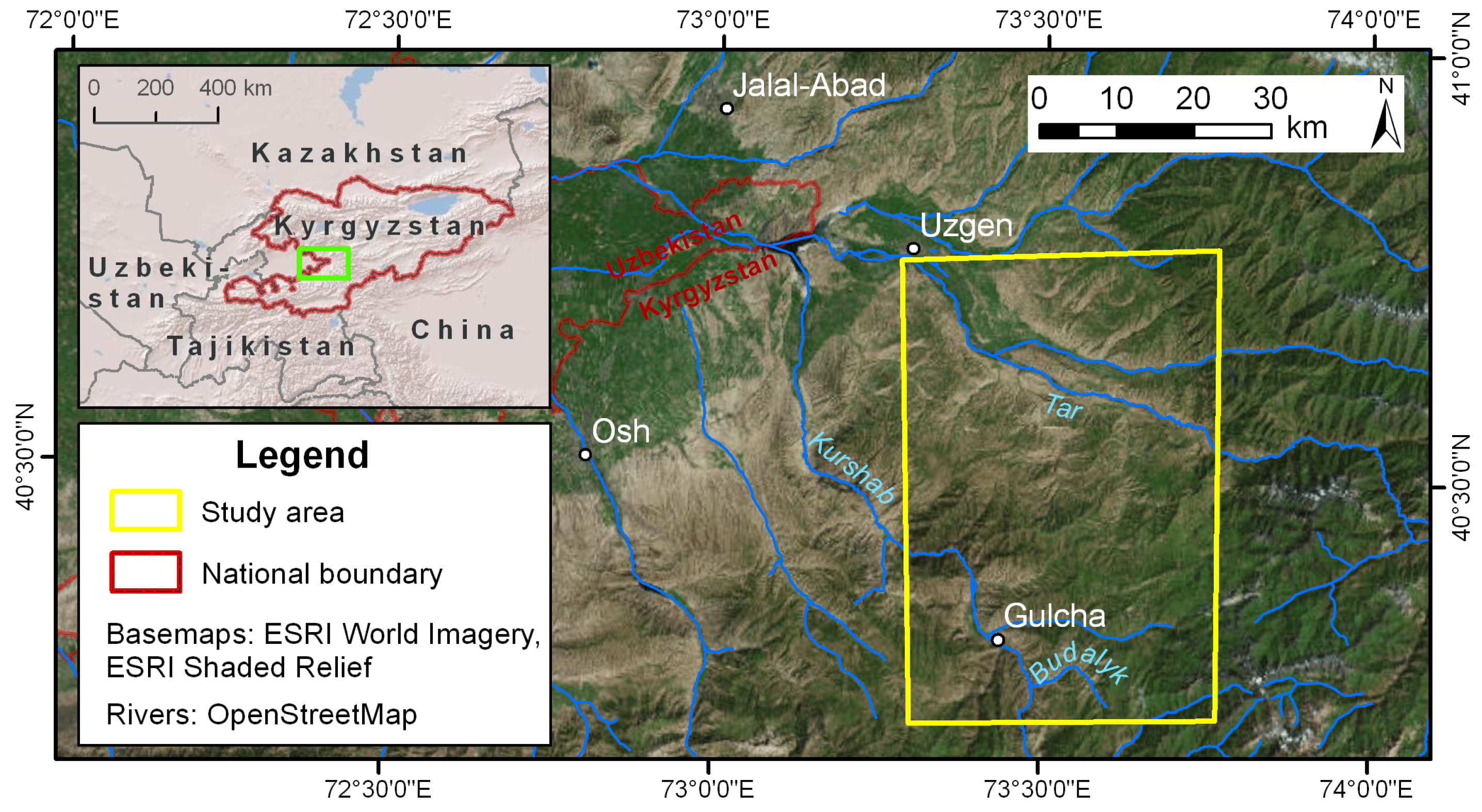
2.1. Study Area

The approximately 60-by-40-km-large study area is located in Osh Province (oblast) of Kyrgyzstan (Figure 1) at the foothills of the Tian Shan. This territory is primarily composed of weakly consolidated Mesozoic and Cenozoic rocks, which have been folded by subsequent tectonic deformations, thus contributing to their instability. Loess cover of varying thickness is deposited in the folds, which leads to particularly fast and dangerous slope failures. Rather than being associated with individual triggering events, most landsliding in the study area occurs in the spring months with significant variations in landslide intensity among the years. These variations have been linked to snow accumulation in the winter months, intensity of snow melting and additional precipitation during the snow melt [18,19].

Earthquakes contribute to the destabilization and can act together with the hydrometeorological factor [20].

The study area is a part of a larger region (approximately 12,000 km² in size) that is affected by intensive landsliding. If the hazard analysis is to be extended to the larger area, then the automated detection allows the analysis to be extended with less effort compared to the expert identification, which would be practically as labor intensive as it was in the smaller study area. In this case, it is important to know whether the quality of the analysis based on the automated detection results is different from that of the analysis based on the expert interpretation results.

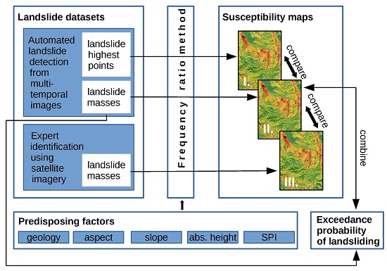
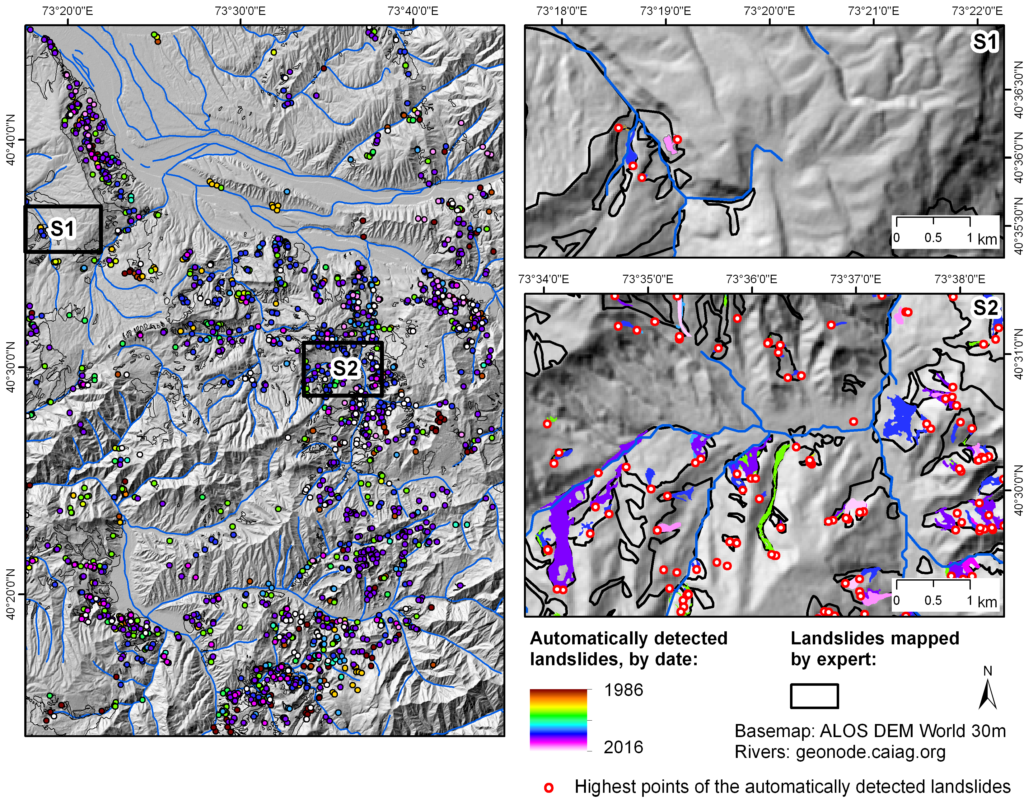
2.2. Landslide Inventory

Regular landslide monitoring in southern Kyrgyzstan was conducted by the local authorities until 1991, with a substantial decrease in the 1990s followed by a gradual resumption. To characterize the landslide activity in the region as fully as possible, multiple information sources need to be combined, each with its strengths and limitations [16,17]. The landslide datasets used in this study were prepared using two different methods:

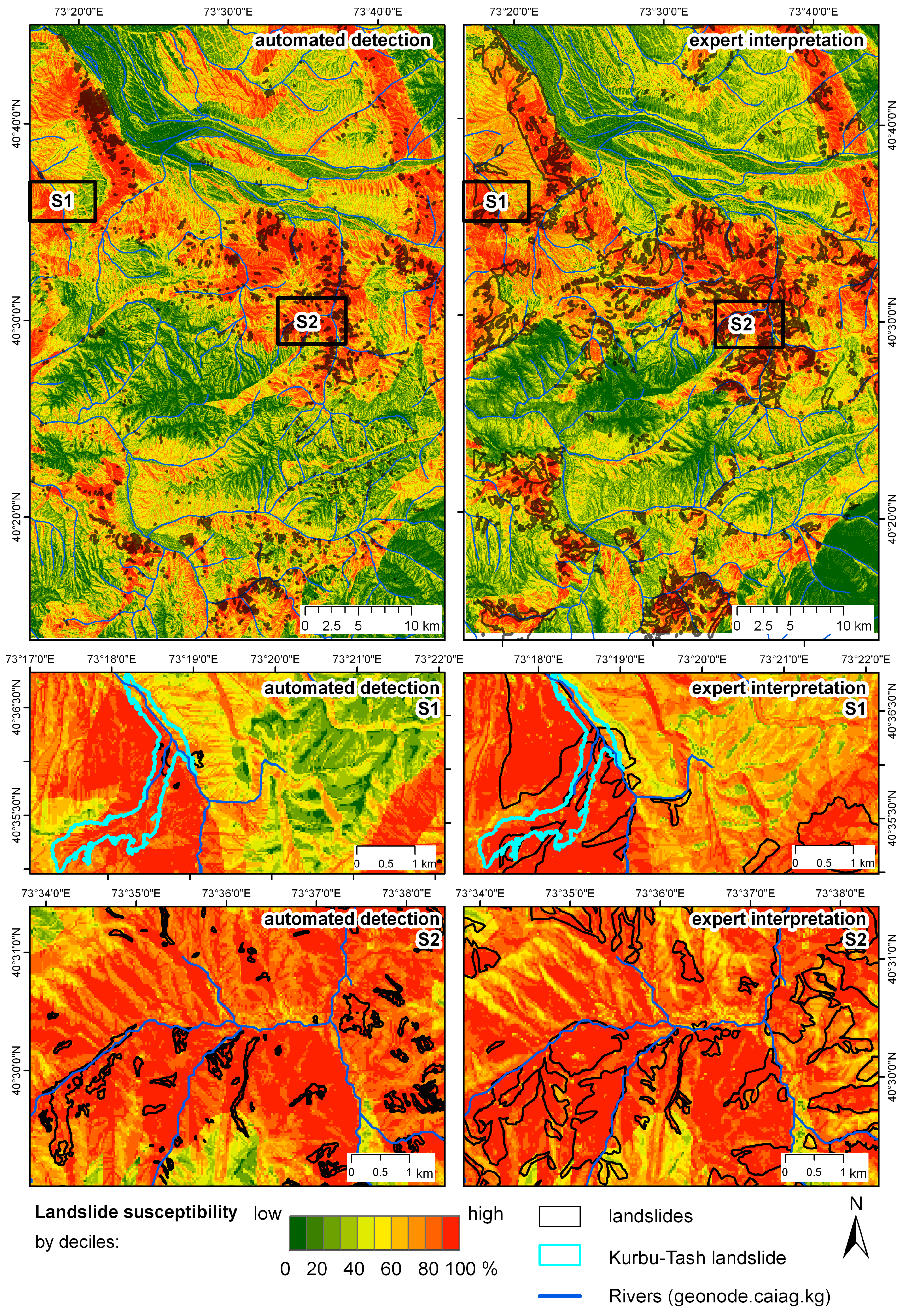
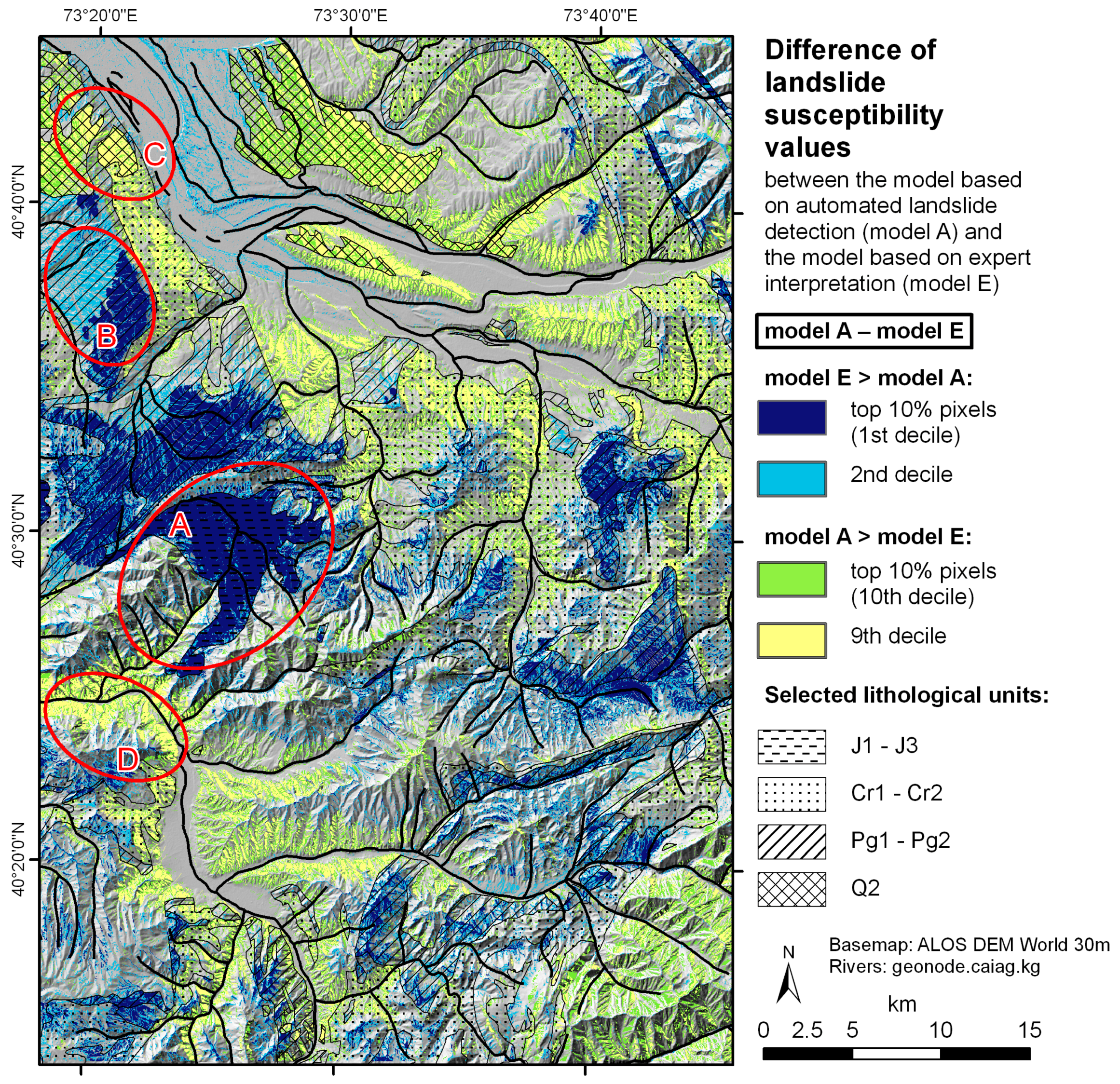
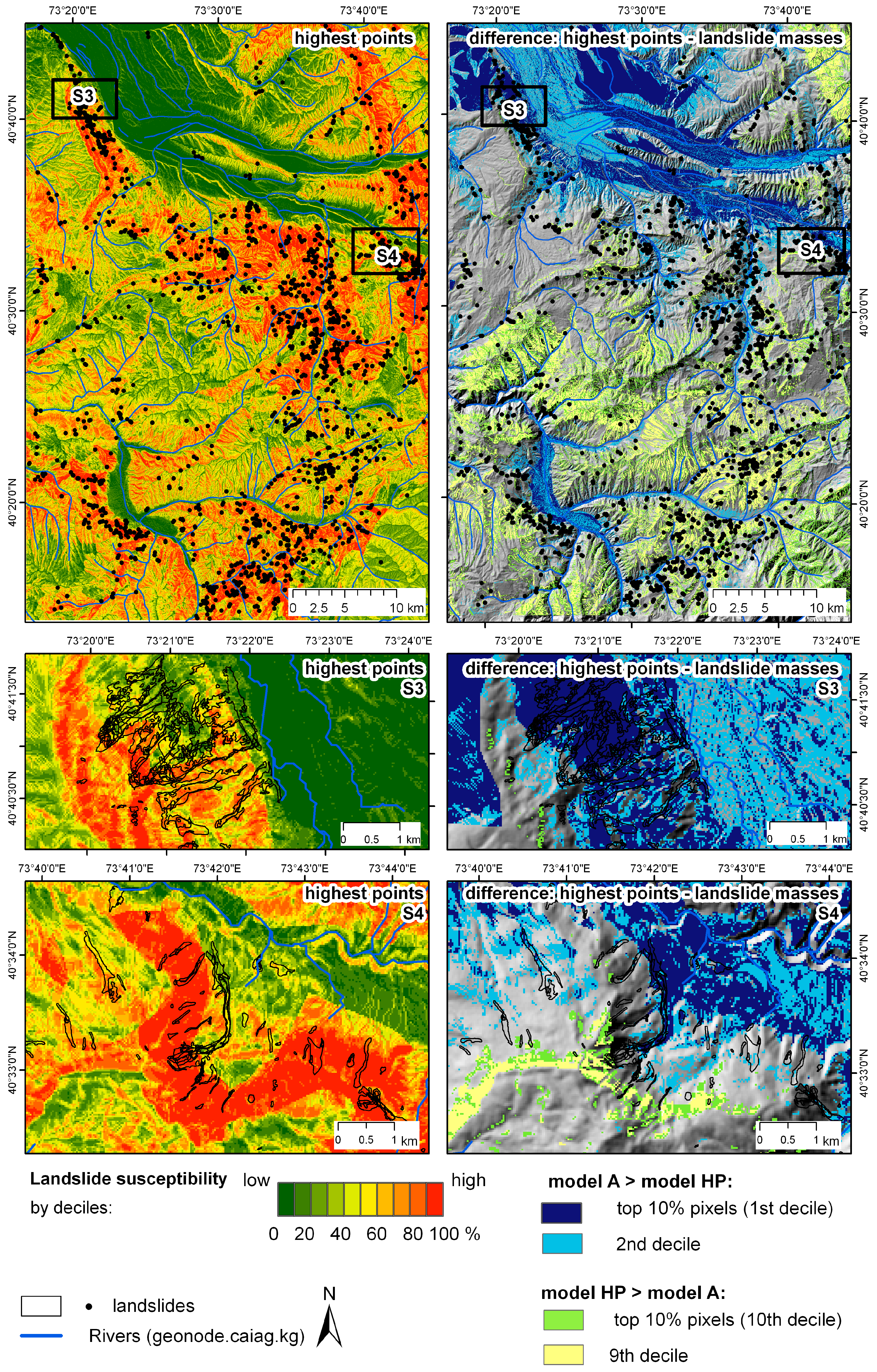
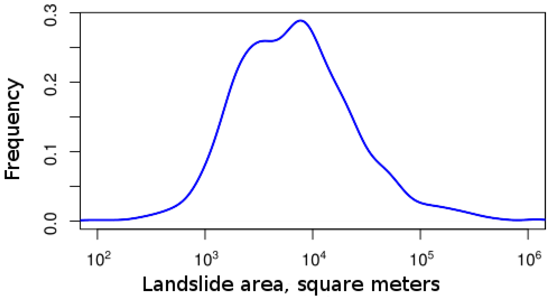
• Automated detection. This dataset was obtained using an automated object-oriented landslide mapping approach that utilizes multi-temporal satellite-based imagery acquired by different optical sensors (Landsat E(TM), SPOT 1-5, ASTER, IRS-1C LISS III, and RapidEye) between 1986 and 2016 [1,2,3,21]. The resulting landslide dataset is composed of 1846 polygons. Each polygon represents the spatial extent of an individual landslide failure. For each landslide polygon, the date of occurrence was determined as the period between two consecutive image acquisitions (before and after the slope failure). The temporal resolution depends on the length of the period between the before and after images. The resolution varies between several years at the beginning and a few weeks at the end of the time span covered by the multi-temporal remote sensing database. The polygons overlap if multiple failures occurred within the same slope over time, which makes it possible to reconstruct the history of landslide reactivations. The resulting dataset is a systematic record of the landslides in the study area that occurred during the past 30 years. This may appear to be a short landslide record, particularly compared to some European countries with very extensive spatial data on landsliding. However, for southern Kyrgyzstan, this dataset is of unprecedented quality and completeness. The length of the period covered by this dataset will increase as new high-resolution satellite images are acquired, but an evaluation of the properties of the dataset and its influence on the susceptibility results can already be performed with the 30-year coverage.
• Expert interpretation. Areas that experienced landsliding in the past and that still exhibit morphological evidence of these past slope failures were mapped visually by an expert. The mapping was based on RapidEye images acquired between 2012 and 2015, a digital elevation model (DEM) and geological information. The resulting dataset represents the cumulative result of landsliding with no information on the failure dates and without the differentiation of the spatial extents of individual activations. Thus, in contrast to the automatically detected dataset, the results of expert interpretation do not contain individual landslide objects but rather a mask that shows whether the given location was affected by landsliding in the past.

The area covered by the expert interpretation dataset is seven times the size of the area covered by the automatically detected dataset (

Table 1. Landslide area documented in the two landslide datasets.

Dataset	Area, km2	Portion of Study Area, %
Landslide area according to the results of automated detection	28.5	1.23
Landslide area as interpreted by the expert	197.8	8.52
Overlapping landslide area of both datasets	19.8	0.86
Area not affected by landsliding in either dataset	2115.0	91.10

). Approximately two thirds of the landslide-affected area of the automatically detected dataset falls into the results of the expert interpretation. Figure 2 shows the spatial distribution of the landslides in the study area and its two subsets. Subset S1 experienced little landsliding over the past 30 years, whereas subset S2 was affected by high landslide activity. Overall, large parts of the study area are subjected to ongoing landslide activity, which is particularly high in several landslide hotspots.

2.3. Predisposing Factors

The data on the landslide predisposing factors are available in the form of a geological map and the Advanced Land Observation Satellite (ALOS) DEM World with a 30 m resolution [22]. The geological map was created through expert reinterpretation of multiple digitized 1:200,000 geological paper maps published prior to 1991. Because a lithological map of the study area is unavailable, we use the structural geological units to characterize the lithology. The following structural units are distinguished (following [23]):

• Basement: Metamorphic and igneous rocks;
• Jurassic (J1–J3): Sandstones, siltstones, and slates;
• Upper Cretaceous—Paleogene (Cr1–Cr2): red sandstones, conglomerates, gravels, gypsolytes, limestones, clays, and siltstones;
• Lower Eocene—Oligocene (Pg1–Pg2): sandstones, gypsolytes, limestones, marls, clays, and siltstones;
• Oligocene—Miocene (Pg3–N1): red sandstones, conglomerates, and clays;
• Pliocene (N2): conglomerates, gravels, and loess-type loams;
• Lower Quaternary (Q1): gray conglomerates and loesses;
• Middle Quaternary (Q2): glacial moraines, loesses, and alluvial sediments;
• Upper Quaternary (Q3–Q4): alluvial sediments, glacial moraines, and loesses.

The open source software packages SAGA GIS (version 2.2.7) and QGIS (version 2.14.3) were used to derive the following factors from the ALOS DEM for each raster cell using its 8-cell neighborhood:

• Aspect shows the exposition of the slope, classified into eight cardinal and intercardinal directions.
• Slope characterizes the steepness of the slope.
• Stream power index (SPI) is a function of the product of flow accumulation and the local slope that describes the potential erosion power at a specific point of the surface [24,25].

3. Methods

Landslide susceptibility indicates how likely a landslide is to occur at a location with a certain combination of predisposing factor values [4,7]. We calculate the landslide susceptibility for both landslide datasets: the results of automated detection and expert interpretation. For the former dataset, we perform the susceptibility analysis (i) using all of the landslide extents and (ii) using a single point at the landslide initiation zone (cf. Section 3.4). We compare and validate the results. Finally, we calculate the exceedance probability of landsliding using the multi-temporal inventory.

3.1. Frequency Ratio Method

In our study, we use the frequency ratio method [26,27]. This method calculates the frequency ratio value for each factor class by comparing the landslide density within that class to the average landslide density in the study area:

$$F{R}_{\mathrm{i}}=\frac{N_{\mathrm{pix}\left({\mathrm{S}}_{\mathrm{i}}\right)}/N_{\mathrm{pix}\left({\mathrm{N}}_{\mathrm{i}}\right)}}{\sum N_{\mathrm{pix}\left({\mathrm{S}}_{\mathrm{i}}\right)}/\sum N_{\mathrm{pix}\left({\mathrm{N}}_{\mathrm{i}}\right)}},$$

(1)

where

• $N_{\mathrm{pix}\left({\mathrm{S}}_{\mathrm{i}}\right)}$ is the number of landslide pixels in each class i;
• $N_{\mathrm{pix}\left({\mathrm{N}}_{\mathrm{i}}\right)}$ is the total number of pixels that have class i in the study area;
• $\sum N_{\mathrm{pix}\left({\mathrm{S}}_{\mathrm{i}}\right)}$ is the total number of landslide pixels in the study area;
• and $\sum N_{\mathrm{pix}\left({\mathrm{N}}_{\mathrm{i}}\right)}$ is the total number of pixels in the study area.

The class boundaries for each factor are determined by the researcher prior to the calculation based on expert knowledge and the data distribution. The landslide susceptibility index (LSI) is then calculated by adding the frequency ratio of each factor for the given pixel. To ensure comparability between susceptibility models with different numbers of factors, the sum is divided by the number of factors:

$$LSI=\frac{1}{n}\sum _{i=1}^{n}F{R}_i\Rightarrow LSI=\frac{FR\left(geology\right)+FR\left(aspect\right)+FR\left(slope\right)+FR\left(absoluteheight\right)+FR\left(SPI\right)}{5}.$$

(2)

3.2. Validation of Susceptibility Assessment

To evaluate the susceptibility models, we use receiver operating characteristic (ROC) curves, which plot the model sensitivity (i.e., the portion of known landslide pixels correctly classified as susceptible) against its specificity (i.e., the portion of landslide-free pixels correctly classified as not susceptible) [28,29]. The area under the curve (AUROC) varies between 0.5 and 1.0, with higher values indicating a better fit of the model. The model is validated by comparing it to a landslide dataset that is not used for calibrating the model [30,31]. The subdivision of the landslide data into the training and validation parts is generally performed randomly or using non-overlapping temporal or spatial subsets of the landslide inventory [30].

We use the following pairs of training and validation datasets:

• The datasets obtained by automated detection (both the landslide highest points and the landslide masses) are divided into training and validation parts. This is a standard approach for validating the susceptibility results when a single landslide dataset is available [29,30]. We divide the datasets into 50%/50% parts.
• The expert interpretation dataset is used for training the model, and the automated detection dataset (landslide masses) is used for validating the model. The goal is to understand whether the automatically detected dataset, which is based on a relatively short 30-year observation period, is capable of producing results that are comparable to the labor-intensive geomorphological mapping.
• The automated results of 2009–2016 (landslide masses) are used to train the model, and the automatic detection dataset of 1986–2009 is utilized to validate the model. This is an attempt to evaluate the reliability of the susceptibility mapping in a scenario where only RapidEye satellite images are available.

3.3. Temporal Probability of Landsliding

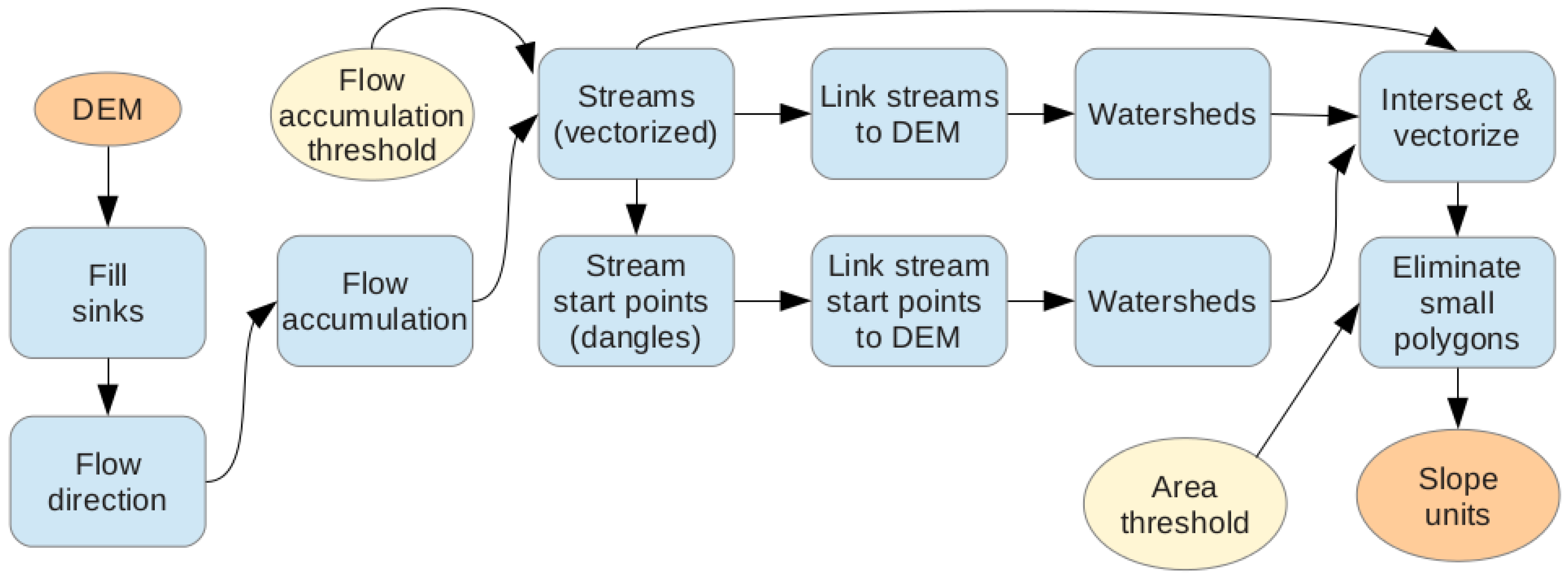
To explore the spatial variations in the landslide activity in time, we calculate the exceedance probability of landslide occurrence using a binomial distribution, as follows:

$$P=1-e^{-\lambda t},$$

(3)

where $\lambda$ is the annual landslide frequency (per mapping unit) and t is the length of the period (in years) for which the exceedance probability is calculated [4,32].

The completeness of a landslide inventory is crucial for the correctness of the exceedance probability calculations because the omission of landslides from the underlying inventory leads to an underestimation of the hazard. However, the completeness of landslide inventories is limited, particularly in data-scarce regions. Landslide size-frequency behavior follows a power law distribution with a roll-over for smaller events [33,34], which is a result of the incomplete mapping of landslides below a certain size. Prior to calculating the exceedance probability of landsliding, we assess the completeness of the automated landslide detection results based on their size-frequency distribution.

3.4. Mapping Units

Mapping units are a result of partitioning the space into non-overlapping parts that together cover the territory of the study area in question. These units are used to transition from discrete and possibly overlapping landslide objects to analyses at the scale of the study area, e.g., in the course of the landslide hazard assessment (cf. [29,35,36]).

In this study, the susceptibility calculation is performed on the basis of 30-m pixels for both landslide datasets. The complete extent of the landslide mass is rasterized and used as the input data for the susceptibility analysis. Additionally, we calculate the susceptibility using a single point for each landslide of the automatically detected dataset. The point representative of the landslide polygon should be located in the landslide initiation zone. To automate the process, we use the highest point within the landslide as an approximation of the landslide main scarp. The highest point is calculated by clipping the DEM raster to the landslide polygon in question and using the center of the pixel that has the highest elevation value. The procedure is automatically performed as a part of the QGIS plugin Landslide Tools [37] implemented by one of the authors. The susceptibility calculation using the highest points cannot be performed with the results of expert interpretation because this dataset does not distinguish between individual landslide objects. The choice of the landslide representation determines the interpretation of the resulting susceptibility model: the model based on the landslide highest points indicates the likelihood of a pixel to initiate a landslide, whereas the model based on complete landslide extents represents the likelihood of the given location to be affected by a landslide.

It is possible to calculate the exceedance probability in a similar pixel-based manner. However, a typical landslide-prone slope in the study area is characterized by recurring landslide failures. Each slope failure may only occupy a part of the slope, whereby the multitude of such events over the years eventually affects the entire slope. The differentiation in the landslide frequency on such slopes is often a result of the short observation period. The absence of landslides in the inventory in the presumably unaffected parts of such slopes does not imply that these areas are safe. In fact, the opposite may be true in the short term. We solve this contradiction by introducing larger mapping units. In this study, slope units have been used as mapping units because they reflect the physical properties of the relief as a major landslide predisposing factor.

We derived the slope units from digital elevation data using an approach based on watershed delineation in ArcGIS. A simplified overview of the approach is presented in Figure 3. We followed the standard ArcGIS procedure, which consists of deriving the stream network by setting a threshold on the flow accumulation raster and then using the branch-off points of the resulting streams to delineate individual watersheds. However, the result of this procedure does not allow distinguishing between opposite slopes of a river valley that touch the same stream segment. Therefore, an additional step was introduced. This step subdivides the watersheds obtained in the previous step into two polygons by intersecting them with the stream lines. For upstream watersheds, an additional third sub-watershed is delineated that drains to the highest point of the stream and represents the uppermost part of the river valley. This approach allows for a more consistent aspect within the resulting slope units. This modified procedure includes two user-defined parameters: the flow accumulation threshold and the area threshold. The flow accumulation threshold is used to vary the size of the resulting slope units to account for the properties of the study area and the scale of the analysis. The area threshold serves to remove resulting polygons that are too small to represent a slope by merging them with their larger neighbors. We assign each landslide to a slope unit based on the location of the landslide highest point.

In the final step, we combine the spatial and temporal aspects into a landslide hazard index, which is done at the level of the slope units using the susceptibility map based on the automatically detected landslide masses. We reclassify the susceptibility map into three classes of equal size (tertiles). The “Majority” function of the QGIS Zonal Statistics tool is used to determine the prevalent susceptibility tertile for each slope unit. From the slope units with the highest susceptibility tertiles, we select the units that have experienced multiple (at least two) landslide failures since 1998. We consider these slope units to have the highest landslide hazard index.

4. Results

4.1. Landslide Susceptibility

4.1.1. Model Results

The frequency ratio values were calculated for all three of the landslide datasets (

Table 2. Frequency ratio values of the predisposing factors by landslide data source. Classes with frequency ratio values > 1 are more favorable for the development of landslides than the study area on average.

Factor	Class	Automated Detection 1986–2016, Highest Points	Automated Detection 1986–2016, Landslide Masses	Expert Interpretation
Geology	Basement	0.281	0.131	0.228
	J1–J3	0.588	0.289	1.345
	Cr1–Cr2	2.134	2.309	2.070
	Pg1–Pg2	1.214	0.956	1.370
	Pg3–N1	1.325	0.646	0.507
	N2	0.622	0.443	0.129
	Q1	0.176	0.030	0.053
	Q2	0.478	1.923	0.954
	Q3–Q4	0.426	0.806	0.973
Aspect	North	1.415	1.382	1.479
	Northeast	1.742	2.108	1.668
	East	1.242	1.423	1.343
	Southeast	0.750	0.705	0.847
	South	0.431	0.423	0.659
	Southwest	0.463	0.435	0.483
	West	0.616	0.542	0.558
	Northwest	1.250	0.964	0.991
Slope, degrees	<5	0.079	0.395	0.518
	5–<10	0.259	1.035	1.395
	10–<15	0.490	1.283	1.640
Slope, degrees	15–<20	0.938	1.347	1.376
	20–<25	1.474	1.137	0.998
	25–<30	1.832	0.968	0.704
	30–<35	1.872	0.760	0.424
	35–<40	1.456	0.610	0.244
	40–<45	1.689	0.796	0.198
	≥45	1.601	0.998	0.152
Absolute height, m	<1200	0.243	0.767	0.694
	1200–<1400	0.305	1.277	0.860
	1400–<1600	0.760	1.658	1.040
	1600–<1800	1.500	1.929	1.492
	1800–<2000	1.706	1.686	1.393
	2000–<2200	1.400	0.749	1.228
	2200–<2400	0.935	0.316	0.962
	2400–<2600	0.433	0.161	0.366
	≥ 2600	0.104	0.027	0.042
SPI	<4	0.044	0.183	0.297
	4–<6	0.456	0.579	0.901
	6–<7	0.889	0.812	0.989
	7–<8	1.412	1.129	1.015
	≥8	1.609	1.887	1.349

). The predisposing factor datasets were reclassified according to these frequency ratio values. To evaluate the ability of individual factors to differentiate between pixels with high and low susceptibilities, the AUROC values of susceptibility models based on a single factor were calculated (

Table 3. Discrimination ability of predisposing factors: area under the receiver operating characteristic (AUROC) curve values of susceptibility models based on a single factor.

Factor	Automated Detection 1986–2016, Highest Points	Automated Detection 1986–2016, Landslide Masses	Expert Interpretation
Geology	0.6960	0.7232	0.7221
Aspect	0.6265	0.6615	0.6303
Slope	0.6820	0.5876	0.6486
Absolute height	0.6560	0.6912	0.6270
SPI	0.6354	0.6318	0.5605

). Geology is the main factor determining the differentiation of landslide susceptibility in the study area in each of the three models. This factor is responsible for the most global level of the study area zonation because it is indicative of the different structural settings of its parts. In the northern part of the study area in particular, the main differences between susceptibility values can be linked to the boundaries of lithological units. Cretaceous deposits (Cr1–Cr2) are consistently the most affected geology class across all three models. The model based on the results of expert interpretation assigns higher susceptibility to Jurassic rocks (J1–J3). The model that uses the automatically detected landslide masses results in high frequency ratio values for Middle Quaternary deposits (Q2). This result is due to the extensive landsliding on the Uzgen slope, where the areas severely affected by landsliding were classified as Q2 in the geological map. The aspect factor behaves similarly among all three of the models. The model based on the landslide highest points assigns higher frequency ratio values for steeper slopes and higher terrain than the other models.

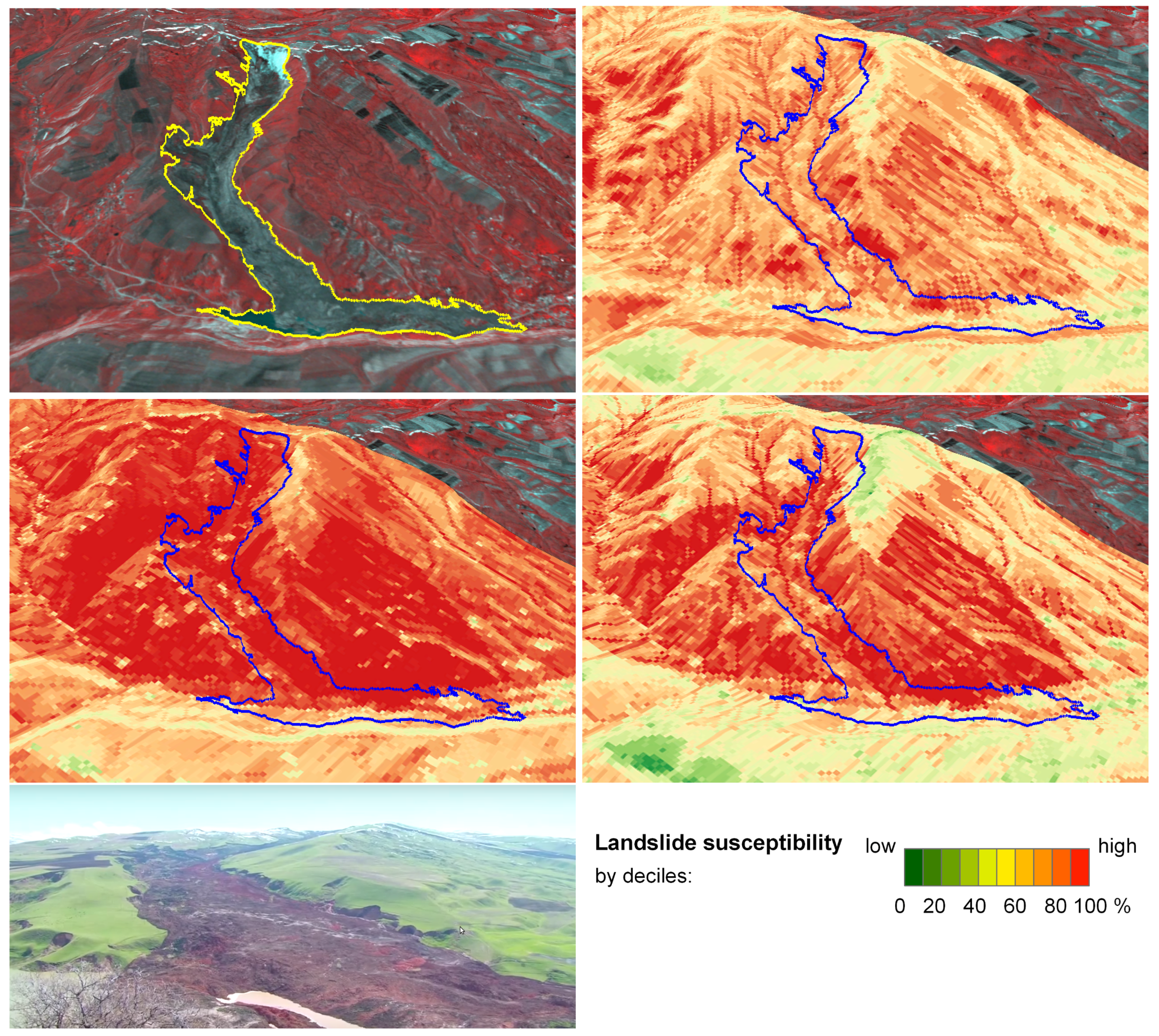
4.1.2. Comparison of Susceptibility Maps: Automated Detection vs. Expert Interpretation

Figure 4 shows the susceptibility maps produced for both landslide datasets. Both susceptibility maps are similar in subset S2. In subset S1, the model based on the automatically detected landslides shows lower susceptibility levels than the model based on the results of expert interpretation.

To compare the susceptibility values of both maps, their difference was calculated (Figure 5). The differences between the two maps can be linked to the frequency ratio values of the predisposing factor classes in both susceptibility models (see Table 2). For example, the automatically detected landslides are more rare in Jurassic and Paleogene deposits than landslides mapped by the expert. Consequently, these areas received lower susceptibility in the model based on the automated detection results (see highlighted areas A and B in Figure 5). The very active slope near the town of Uzgen in the very northwest of the study area (highlighted area C in Figure 5) has a substantial influence on the susceptibility model based on the automatically detected landslides. The consequence is a large frequency ratio value for northeastern slopes in the susceptibility model based on automatically detected landslides. This reflects not only on the Uzgen slope itself but also in other parts of the study area, e.g., highlighted area D in Figure 5. No landslides have been recorded in highlighted area D, but a visual assessment of the satellite imagery from Google Earth (by Google Inc., Mountain View, California) indicates that landsliding is plausible here.

4.1.3. Comparison of Susceptibility Maps: Landslide Masses vs. Highest Points

The differences between the susceptibility models based on the landslide highest points and the landslide masses reflect the nature of the input data. The model calculated using the highest points assigns higher susceptibility values to upper parts of the slope (e.g., subset S4 in Figure 6). Furthermore, it results in lower susceptibility for Middle Quaternary (Q2) deposits (e.g., the Uzgen slope in subset S3 in Figure 6) and higher susceptibility for areas with more consolidated rocks due to the higher elevation and slope values there. Landslides in the areas with more consolidated rocks are small, but because the landslide size has no influence on the susceptibility model based on landslide highest points, small landslides receive more weight in this model.

4.1.4. Validation

After selecting the best susceptibility models, we assess their predictive power in a validation procedure. We also use this opportunity to analyze how the input landslide data quality affects the susceptibility assessment results.

The AUROC values presented in

Table 4. Validation results.

Row	Training Dataset	Validation Dataset	AUROC *
1	Automated detection 1986–2016, highest points (50%)	Automated detection 1986–2016, highest points (50%)	0.7998
2	Automated detection 1986–2016, landslide masses (50%)	Automated detection 1986–2016, landslide masses (50%)	0.8142
3	Expert interpretation	Automated detection 1986–2016	0.7730
4	Automated detection 2009–2016, landslide masses	Automated detection 1986–2009, landslide masses	0.8053

* area under the receiver operating characteristic curve.

suggest that the susceptibility mapping results are acceptable for all the landslide datasets. The highest values were achieved using the landslide masses detected automatically in 1986–2016. Even the shorter dataset covering the period between 2009 and 2016 with high-resolution RapidEye images results in an AUROC value of 0.8. This result implies that the susceptibility assessment can be extended to the territory adjacent to our study area, provided that RapidEye images are available.

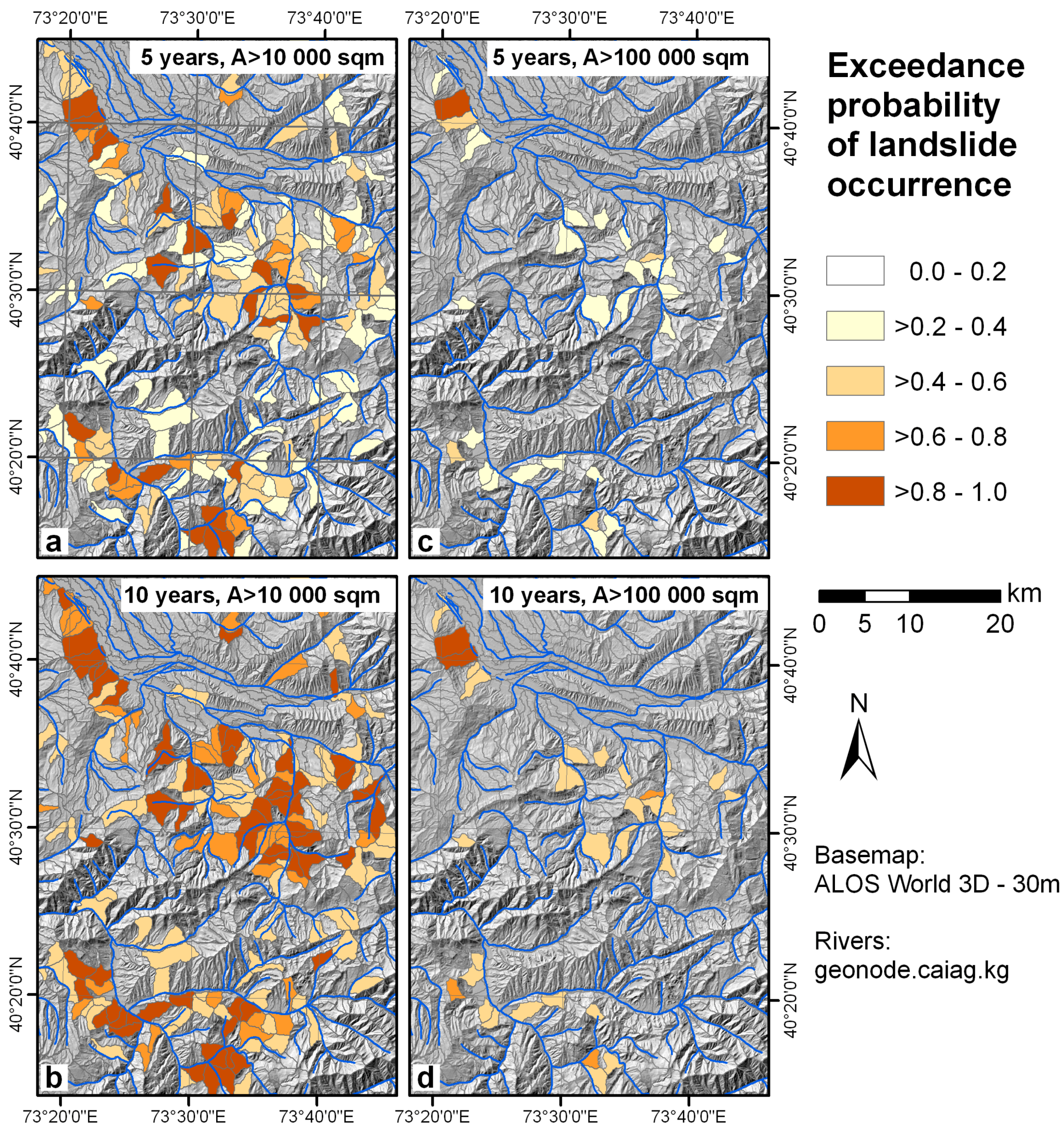
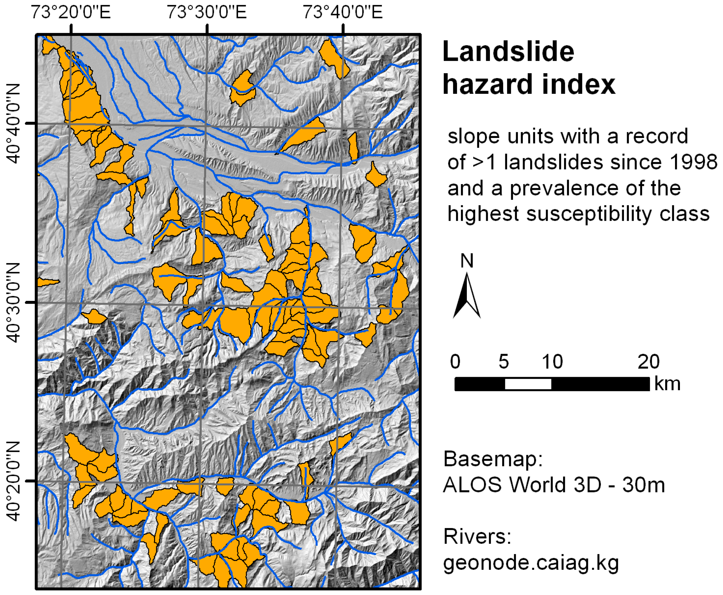
4.2. Temporal Probability of Landsliding

We calculated the exceedance probability of landsliding using the results of automated landslide detection. This dataset covers the 30-year period between 1986 and 2016. According to data from the local authorities, the year 1994 experienced an exceptional number of landslides in southern Kyrgyzstan: a third of all slope failures registered from 1986–2010 occurred in 1994 [18]. However, this exceptional landslide activity is not reflected in the automated detection results. The automatically detected landslide dataset contains 1846 landslides, but only 164 of them failed in 1986–1998. One reason for this result is that the statistics from the local authorities refer to a territory that is larger than our study area, and the hotspot of landslide activity in 1994 was north of the study area. However, a more important reason is the low temporal resolution of the imagery used for the automated detection. The earliest image acquisition dates were in 1986, 1990 and 1998. The interval between 1990 and 1998 is so long that some of the slope failures could not be detected using remote sensing due to revegetation and/or subsequent failures on the same slope during the same time period. This is, e.g., the case for the landslide in the Kandava river valley next to the village of Komsomol that failed on 26 March 1994 and caused 28 fatalities [18]. Furthermore, the spatial resolution of the images available for the early periods is lower and thus simply does not enable smaller landslides to be detected. To avoid an underestimation of landslide hazard, we only use landslide data of 1998–2016 in the following analysis of the temporal component.

The assessment of the size-frequency distribution for these landslides (Figure 7) shows a roll-over effect in the probability density curve for landslide areas under 10,000 m². Therefore, the available data permit the calculation of the exceedance probability only for landslides of this size or larger.

The exceedance probabilities of the occurrence of landslides larger than 10,000 m² for periods of 5 and 10 years are presented in Figure 8a,b. The exceedance probability of landslide occurrence for the period of 5 years is over 80% on the Uzgen slope, in parts of the basins of left tributaries of the Tar river, around the village of Gulcha and in the Budalyk river valley. Large landslides over 100,000 m² are particularly likely on the Uzgen slope (Figure 8c,d).

After combining the exceedance probability map with the susceptibility map based on the automated landslide detection results (landslide masses), we select the slope units with the highest landslide index (Figure 9). They largely coincide with the distribution of the main landslide hotspots in the study area.

5. Discussion

We have calculated landslide susceptibility for the study area in southern Kyrgyzstan using two versions (highest points of landslide initiation and complete landslide masses) of a multi-temporal landslide inventory and a historical landslide inventory and five predisposing factors (geology, aspect, slope, absolute height and stream power index). The multi-temporal inventory was generated by automated landslide detection from time series of optical satellite images covering the period between 1986 and 2016. The historical inventory was derived by expert mapping using a combination of satellite remote sensing interpretation and already existing knowledge on landslide occurrence.

The good performance (AUROC values between 0.77 and 0.81) of the models for all three types of landslide input data and a visual assessment of the resulting maps indicate that the automated landslide detection method is a valid and more precise alternative to the labor-intensive manual mapping. Although the quantitative AUROC metrics are commonly accepted for quality assessment within landslide susceptibility studies, they need to be complemented with an assessment of the potential biases contained in the input landslide and factor data and of geomorphic plausibility checks [38]. Moreover, the results of susceptibility analysis should be compared to independent landslide occurrences, e.g., slope failures of 2017.

The differences in the susceptibility values of individual factor classes between the historical and multi-temporal inventories can be traced back to the fact that the landslides mapped by the expert occupy a larger area and span over a wider range of natural conditions and a longer time period of occurrence. This explains why some factor classes (e.g., Jurassic and Paleogene rocks) are represented with a higher significance in the model based on the landslide inventory derived by the expert compared to the inventory derived by automated remote sensing analysis. We conclude that the recurrence intervals of landslides in such areas exceed the 30-year-long time period for which satellite remote sensing time series data of sufficient spatial resolution are available for the study area.

The spring of 2017, which is not yet covered by the inventory used in this study, represents an extraordinary period of landslide activity caused by a threefold increase in winter precipitation between October and March compared to the long-term average [39]. These extraordinary meteorological conditions led to the activation of a high number of landslides of partially very large extent. Within our study area, a 4.3-km-long landslide occurred at the end of April 2017 near the village of Kurbu-Tash, destroying approximately 60 houses whose residents had been evacuated prior to the main failure (Figure 10) [40,41]. The landslide occurred on a slope within subset S1 of the study area (Figure 4), which had not been affected by landsliding over the past 30 years. However, the expert-based landslide mapping had revealed morphological indicators of ancient landsliding, which were included in this inventory. Nevertheless, both susceptibility maps depict the highest susceptibility values for similar regions and are characterized by acceptable to high predictive performances.

Overall, the multi-temporal landslide inventory results in a susceptibility assessment that better reflects the landslide properties observed in recent decades. Whether this is an advantage or a disadvantage also depends on the ratio between the length of the observation period and the landslide recurrence intervals in the study area. The model based on the inventory derived by automated detection underestimates the susceptibility of predisposing factor combinations that are only activated under conditions not observed over the past 30 years. However, the automated approach does not require the involvement of a landslide expert who is capable of performing the manual landslide mapping. Therefore, it can be used to generate an inventory that is suitable for an initial susceptibility assessment, which can then be further evaluated.

Moreover, in the case of a large area of interest, the derivation of a historical inventory may be too labor intensive to perform. In contrast, the detailed analysis of a smaller area may require a spatially more focused inventory incorporating all available information sources, whereas the automated inventory allows outlining those parts of the study area that are characterized by the highest recent landslide activity. Therefore, we consider both types of inventories as valuable information sources on landslide occurrence that complement each other, and both need to be considered in a comprehensive susceptibility analysis.

When comparing the susceptibility models resulting from incorporating different landslide properties—polygon-based whole landslide masses versus the point-based approximation of landslide initiation zones—a spatial shift of higher susceptibility values toward the more elevated parts of the slope is observed. Moreover, the susceptibility model based on highest points is biased toward small landslides because they receive the same weight in the model as very large slope failures. In the study area, small landslides are mostly found in more consolidated rocks (which are less likely to experience highly hazardous slope failures), whereas the weakly consolidated sediments produce the largest and most dangerous landslides. Thus, the approach based on highest points effectively underestimates the hazard in the most affected areas. Therefore, the susceptibility model based on whole landslide masses also needs to be considered. The two susceptibility models can complement each other and should both be taken into account for comprehensively characterizing the different aspects of landslide susceptibility. This also points to the advantage of GIS-based landslide susceptibility and hazard assessment over conventional expert-based mapping approaches consisting of the flexible consideration of different input information for deriving a variety of complementary models that can be further evaluated by landslide experts.

This situation is also illustrated by the example of the Kurbu-Tash landslide. For both susceptibility models (expert and automated) that are based on the use of landslide masses, the susceptibility values within the area of the Kurbu-Tash landslide are rather high: a large part of the area covered by the landslide belongs to the 20% of the study area that is characterized by the highest susceptibility. In contrast, the model that uses the highest point of landslide initiation results in lower susceptibility values for the area of the Kurbu-Tash landslide. This example shows the effect of using different landslide properties on the model results, leading to an underestimation of the susceptibility originating from large landslides. Moreover, the high landslide activity in 2017 indicates that there is a considerable need for future continuation of systematic large-area landslide monitoring in southern Kyrgyzstan to further improve the susceptibility and hazard assessment.

Due to the availability of the remote-sensing-based multi-temporal inventory, we were able to assess not only the landslide susceptibility but also the exceedance probability of landsliding. This is the first step in analyzing the temporal aspect of the landslide hazard in this region. Further research is needed to link the differences in landslide frequency between the years to changes in the potential triggering factors, such as the hydrometeorological conditions. Once high-resolution multi-temporal imagery are available for a period of several decades for southern Kyrgyzstan, landslide hazard assessments can focus more on the temporal analyses derived from the landslide frequencies. In this case, the analyses will no longer be affected by the scarcity of data on predisposing factors.

For this purpose, future continuation of systematic landslide monitoring in the study area is crucial. It will extend the observation period and possibly include landslide locations with a combination of predisposing factors that have not yet been represented in our susceptibility model [42]. More importantly, the landslide activity in the study area is characterized by occasional very intensive years with a dramatic increase in landslide activity. In such intensive years, landslides may become activated on slopes that have been stable for the past decades and possibly have not been accounted for by the susceptibility model based on the automatically detected data. The results of automated landslide detection have captured the peak in landslide occurrence in 2003–2004 [2], but the landslide activity of the even larger peak of 1994 could not be adequately reconstructed because of the lack of suitable satellite remote sensing data. The continuation of monitoring including the most recent peak year of 2017 and beyond provides an opportunity to improve our understanding of the landslide processes in the study area and is thus the basis for subsequent susceptibility and hazard assessments.

The results of this study show that landslide susceptibility and hazard assessments based on satellite remote sensing are particularly suitable for regions with high process activity and, at the same time, for limited information on landslide occurrence and predisposing factors due to insufficient means for landslide mapping and subsequent hazard analysis. Remote-sensing-based hazard assessment allows the efficient identification of the particularly hazardous areas, which can then be subject to more concentrated monitoring and mitigation efforts. In this context, the recent launches of the Sentinel-2A and 2B satellite remote sensing missions are of crucial importance since they provide satellite imagery of suitable spatial and temporal resolutions at the global scale free of charge, enabling multi-temporal landslide monitoring worldwide. We have already performed the first preliminary investigations on the potential of Sentinel 2A/B to automatically derive landslide failures that occurred during the most recent period of high landslide activity of spring 2017 in southern Kyrgyzstan. The first results indicated a great potential for landslide detection with high spatial detail and completeness over large areas, which will even further increase when the full temporal resolution of the 2A/B Sentinel constellation is enabled worldwide. However, even under the condition of thus far limited revisit time of data acquisition, the principal suitability of these data as a basis for automated derivation of multi-temporal landslide inventories has already been proven.

6. Conclusions

Our investigations have shown that satellite remote sensing can support landslide susceptibility and hazard analysis in multiple ways, particularly for large data-scarce regions such as southern Kyrgyzstan. We have utilized remote sensing at every stage of the investigation, whereas the main emphasis has been placed on the influence of landslide inventory properties on the results of susceptibility and hazard assessments. In our work, we have shown that satellite remote sensing methods can greatly support the expert-based derivation of historical landslide inventories and the derivation of multi-temporal inventories for the entire time period of suitable satellite remote sensing data availability. However, the latter requires the use of automated methods to analyze multi-temporal time series data covering several decades. The resulting systematic spatio-temporal inventories are the main prerequisite for analyzing the temporal component of landslide hazard.

Since both of the derived landslide inventories contain object-based information on past landslide occurrences, we were able to calculate different susceptibility models that emphasize different aspects of landslide activity in the study area. However, for all of these models, AUROC values of approximately 0.8 were achieved. Hence, we conclude that, in our study area, the different models can be used in a complementary way to perform a comprehensive characterization of landslide susceptibility.

The shorter 30-year observation period of the automatically derived multi-temporal inventory results in a susceptibility map with a stronger representation of the properties of the recent landsliding. In contrast, the inventory derived by expert mapping contains a longer time span of landslide occurrence. However, in both susceptibility maps, the highest susceptibility values are observed for similar areas. We conclude that the results of the automated landslide detection provide a suitable landslide inventory for a reliable large-area landslide susceptibility assessment.

We also used the temporal information of the automatically derived multi-temporal landslide inventory to assess the temporal component of landslide hazard in the form of the exceedance probability. Both versions of the susceptibility assessment are useful for showing that the slopes that are more likely to produce a landslide under today’s conditions, as well as areas that may have a high hazardous potential in the future when natural conditions might arise again that have already caused intense landsliding in the past.

Moreover, our investigations have shown that the specific landslide properties used in the susceptibility analysis have a significant influence on the results. If the model is based on the highest point covered by the mapped landslide representing an approximation of the main scarp, then the resulting susceptibility model indicates where landslide initiation is most likely to occur. In contrast, using the complete landslide polygons results in a map that emphasizes the areas that are most likely to be covered by landslide masses. Ideally, both maps should be available to provide a better understanding of both aspects of landslide susceptibility analysis.

The presented approach is based on the extensive use of remote sensing and GIS methods, enabling an objective, quantitative and comprehensive characterization of the different aspects of landslide susceptibility and hazard. The temporal component of landslide hazard can only be assessed if a multi-temporal inventory is available. Our investigations have shown that multi-temporal satellite remote sensing has great potential for deriving such inventories, which will further increase upon the global availability of Sentinel-2A/B data.

References

1. Behling, R.; Roessner, S.; Segl, K.; Kleinschmit, B.; Kaufmann, H. Robust Automated Image Co-Registration of Optical Multi-Sensor Time Series Data: Database Generation for Multi-Temporal Landslide Detection. Remote Sens. 2014, 6, 2572–2600. [Google Scholar] [CrossRef]
2. Behling, R.; Roessner, S.; Golovko, D.; Kleinschmit, B. Derivation of long-term spatiotemporal landslide activity—A multi-sensor time series approach. Remote Sens. Environ. 2016, 186, 88–104. [Google Scholar] [CrossRef]
3. Behling, R.; Roessner, S.; Kaufmann, H.; Kleinschmit, B. Automated Spatiotemporal Landslide Mapping over Large Areas Using RapidEye Time Series Data. Remote Sens. 2014, 6, 8026–8055. [Google Scholar] [CrossRef]
4. Guzzetti, F.; Reichenbach, P.; Cardinali, M.; Galli, M.; Ardizzone, F. Probabilistic landslide hazard assessment at basin scale. Geomorphology 2005, 72, 272–299. [Google Scholar] [CrossRef]
5. Guzzetti, F.; Mondini, A.C.; Cardinali, M.; Fiorucci, F. Landslide inventory maps: New tools for an old problem. Earth Sci. Rev. 2012, 112, 42–66. [Google Scholar] [CrossRef]
6. Van Westen, C.J.; Castellanos, E.; Kuriakose, S.L. Spatial data for landslide susceptibility, hazard, and vulnerability assessment: An overview. Eng. Geol. 2008, 102, 112–131. [Google Scholar] [CrossRef]
7. Corominas, J.; van Westen, C.; Frattini, P.; Cascini, L.; Malet, J.P.; Fotopoulou, S.; Catani, F.; Van Den Eeckhaut, M.; Mavrouli, O.; Agliardi, F.; et al. Recommendations for the quantitative analysis of landslide risk. Bull. Eng. Geol. Environ. 2014, 73, 209–263. [Google Scholar]
8. Fressard, M.; Thiery, Y.; Marquaire, O. Which data for quantitative landslide susceptibility mapping at operational scale? Case study of the Pays d’Auge plateau hillslopes (Normandy, France). Nat. Hazards Earth Syst. Sci. 2014, 14, 569–588. [Google Scholar] [CrossRef] [Green Version]
9. Brenning, A. Spatial prediction models for landslide hazards: review, comparison and evaluation. Nat. Hazards Earth Syst. Sci. 2007, 91, 853–862. [Google Scholar] [CrossRef]
10. Pourghasemi, H.R.; Moradi, H.R.; Fatemi Aghda, S.M. Landslide susceptibility mapping by binary logistic regression, analytical hierarchy process, and statistical index models and assessment of their performances. Nat. Hazards 2013, 69, 749–779. [Google Scholar] [CrossRef]
11. Pradhan, B. A Comparative Study on the Predictive Ability of the Decision Tree, Support Vector Machine and Neuro-fuzzy Models in Landslide Susceptibility Mapping Using GIS. Comput. Geosci. 2013, 51, 350–365. [Google Scholar] [CrossRef] [Green Version]
12. Yilmaz, I. Landslide susceptibility mapping using frequency ratio, logistic regression, artificial neural networks and their comparison: A case study from Kat landslides (Tokat—Turkey). Comput. Geosci. 2009, 35, 1125–1138. [Google Scholar] [CrossRef]
13. Steger, S.; Brenning, A.; Bell, R.; Glade, T. The propagation of inventory-based positional errors into statistical landslide susceptibility models. Nat. Hazards Earth Syst. Sci. 2016, 16, 2729–2745. [Google Scholar] [CrossRef]
14. Pellicani, R.; Spilotro, G. Evaluating the quality of landslide inventory maps: comparison between archive and surveyed inventories for the Daunia region (Apulia, Southern Italy). Bull. Eng. Geol. Environ. 2015, 74, 357–367. [Google Scholar] [CrossRef]
15. Galli, M.; Ardizzone, F.; Cardinali, M.; Guzzetti, F.; Reichenbach, P. Comparing landslide inventory maps. Geomorphology 2008, 94, 268–289. [Google Scholar] [CrossRef]
16. Golovko, D.; Roessner, S.; Behling, R.; Wetzel, H.U.; Kleinschmit, B. Development of Multi-Temporal Landslide Inventory Information System for Southern Kyrgyzstan Using GIS and Satellite Remote Sensing. PFG Photogramm. Fernerkund. Geoinf. 2015, 2, 157–172. [Google Scholar] [CrossRef]
17. Golovko, D.; Roessner, S.; Behling, R.; Kleinschmit, B. Automated derivation and spatio-temporal analysis of landslide properties in southern Kyrgyzstan. Nat. Hazards 2017, 85, 1461–1488. [Google Scholar] [CrossRef]
18. Ibatulin, K.V. Monitoring of Landslides in Kyrgyzstan; Ministry of Emergency Situations of the Kyrgyz Republic: Bishkek, Kyrgyzstan, 2011. (In Russian)
19. Torgoev, I.A.; Aleshin, Y.G.; Meleshko, A.; Havenith, H.B. Landslide hazard in the Kyrgyz Tien Shan. In Proceedings of the Mountain Risks Conference, Firenze, Italy, 24–26 November 2010. [Google Scholar]
20. Danneels, G.; Bordeau, C.; Torgoev, I.; Havenith, H.B. Geophysical investigation and dynamic modelling of unstable slopes: Case-study of Kainama (Kyrgyzstan). Geophys. J. Int. 2008, 175, 17–34. [Google Scholar] [CrossRef]
21. Behling, R.; Roessner, S. Spatiotemporal Landslide Mapper for Large Areas Using Optical Satellite Time Series Data. In Advancing Culture of Living with Landslides; Mikos, M., Arbanas, Z., Yin, Y., Sassa, K., Eds.; Springer International Publishing: Cham, Switzerland, 2017. [Google Scholar]
22. ALOS DEM World—30m. Available online: http://www.eorc.jaxa.jp/ALOS/en/aw3d30/ (accessed on 30 July 2017).
23. Roessner, S.; Wetzel, H.U.; Kaufmann, H.; Sarnagoev, A. Potential of Satellite Remote Sensing and GIS for Landslide Hazard Assessment in Southern Kyrgyzstan (Central Asia). Nat. Hazards 2005, 35, 395–416. [Google Scholar] [CrossRef]
24. Jebur, M.N.; Pradhan, B.; Tehrany, M.S. Optimization of landslide conditioning factors using very high-resolution airborne laser scanning (LiDAR) data at catchment scale. Remote Sens. Environ. 2014, 152, 150–165. [Google Scholar] [CrossRef]
25. Moore, I.D.; Grayson, R.B.; Ladson, A.R. Digital terrain modelling: A review of hydrogical, geomorphological, and biological applications. Hydrol. Process. 1991, 5, 3–30. [Google Scholar] [CrossRef]
26. Lee, S.; Talib, J.A. Probabilistic landslide susceptibility and factor effect analysis. Environ. Geol. 2005, 47, 982–990. [Google Scholar] [CrossRef]
27. Intarawichian, N.; Dasananda, S. Frequency ratio model based landslide susceptibility mapping in lower Mae Chaem watershed, Northern Thailand. Environ. Earth Sci. 2011, 64, 2271–2285. [Google Scholar] [CrossRef]
28. Begueria, S. Validation and Evaluation of Predictive Models in Hazard Assessment and Risk Management. Nat. Hazards 2006, 37, 315–329. [Google Scholar] [CrossRef] [Green Version]
29. Van Den Eeckhaut, M.; Reichenbach, P.; Guzzetti, F.; Rossi, M.; Poesen, J. Combined landslide inventory and susceptibility assessment based on different mapping units: An example from the Flemish Ardennes, Belgium. Nat. Hazards Earth Syst. Sci. 2009, 9, 507–521. [Google Scholar] [CrossRef]
30. Chung, C.J.; Fabbri, A.G. Predicting landslides for risk analysis—Spatial models tested by a cross-validation technique. Geomorphology 2008, 3–4, 438–452. [Google Scholar] [CrossRef]
31. Remondo, J.; Gonzälez, A.; Díaz de Terán, J.; Cendrero, a.; Fabbri, A.; Chung, C.J.F. EValidation of Landslide Susceptibility Maps; Examples and Applications from a Case Study in Northern Spain. Nat. Hazards 2003, 30, 437–449. [Google Scholar] [CrossRef]
32. Corominas, J.; Moya, J. A review of assessing landslide frequency for hazard zoning purposes. Eng. Geol. 2008, 102, 193–213. [Google Scholar] [CrossRef]
33. Havenith, H.B.; Torgoev, A.; Schlögel, R.; Braun, A.; Torgoev, I.; Ischuk, A. Tien Shan Geohazards Database: Landslide susceptibility and analysis. Geomorphology 2015, 249, 32–43. [Google Scholar] [CrossRef]
34. Malamud, B.D.; Turcotte, D.L.; Guzzetti, F.; Reichenbach, P. Landslide inventories and their statistical properties. Earth Surf. Process. Landf. 2004, 29, 687–711. [Google Scholar] [CrossRef]
35. Guzzetti, F.; Carrara, A.; Cardinali, M.; Reichenbach, P. Landslide hazard evaluation: A review of current techniques and their application in a multi-scale study, Central Italy. Geomorphology 1999, 31, 181–216. [Google Scholar] [CrossRef]
36. Erener, A.; Düzgün, H.S.B. Landslide susceptibility assessment: what are the effects of mapping unit and mapping method? Environ. Earth Sci. 2012, 66, 859–877. [Google Scholar] [CrossRef]
37. QGIS Plugin Landslide Tools. Available online: https://github.com/daryagol/landslidetools (accessed on 5 May 2017).
38. Steger, S.; Brenning, A.; Bell, R.; Petschko, H.; Glade, T. Exploring discrepancies between quantitative validation results and the geomorphic plausibility of statistical landslide susceptibility maps. Geomorphology 2017, 262, 8–23. [Google Scholar] [CrossRef]
39. Ministry of Emergency Situations of the Kyrgyz Republic. Reasons for the Activization of Landsliding. Available online: http://mes.kg/ru/news/full/9875.html (accessed on 27 May 2017). (In Russian)
40. AKIpress. Massive Landslide in Osh Region, Kyrgyzstan May 2017. Available online: https://akipress.com/video:651/ (accessed on 27 May 2017).
41. Petley, D. Ayu in Osh, Kyrgyzstan: A Large Landslide Has Killed 24 People, and Another Large Flowslide in Uzgen Region. Available online: http://blogs.agu.org/landslideblog/2017/05/02/ayu-1/ (accessed on 27 May 2017).
42. Wang, Q.; Wang, D.; Huang, Y.; Wang, Z.; Zhang, L.; Guo, Q.; Chen, W.; Chen, W.; Sang, M. Landslide Susceptibility Mapping Based on Selected Optimal Combination of Landslide Predisposing Factors in a Large Catchment. Sustainability 2015, 7, 16653–16669. [Google Scholar] [CrossRef]
Figure 1. Location of the study area.
Remotesensing 09 00943 g001
Figure 2. Landslides in the study area mapped by expert interpretation (black contours) and automated detection (colored polygons and points). The points in the overview map are the centroids of the automatically detected landslide polygons. The representation with points is for visualization purposes only; the actual dataset contains polygons.
Remotesensing 09 00943 g002
Figure 3. Workflow for the derivation of slope units.
Remotesensing 09 00943 g003
Figure 4. Results of susceptibility assessment produced using automatically detected landslide masses (1986–2016) and landslides obtained by expert interpretation: study area and two subsets.
Remotesensing 09 00943 g004
Figure 5. Difference between susceptibility maps produced using the results of automated detection (landslide masses, “model A”) and expert interpretation (“model E”).
Remotesensing 09 00943 g005
Figure 6. Results of susceptibility assessment produced using landslide masses (model A) and landslide highest points (model HP) of automatically detected landslides (1986–2016): study area and two subsets.
Remotesensing 09 00943 g006
Figure 7. Size-frequency distribution of automatically detected landslides in 1998–2016.
Remotesensing 09 00943 g007
Figure 8. Exceedance probability of the occurrence of a landslide with an area over 10,000 m2 (a,b) and over 100,000 m2 (c,d) by slope unit.
Remotesensing 09 00943 g008
Figure 9. Slope units with the highest landslide hazard index, i.e., slope units where (i) more than one landslide failure occurred since 1998 and (ii) the highest susceptibility tertile occupies a larger area than any other tertile.
Remotesensing 09 00943 g009
Figure 10. The 4.3-km-long Kurbu-Tash landslide that occurred in April 2017 (extent determined by automated detection) overlaid over a false-color near-infrared RapidEye image acquired on 2 May 2017 (top left). Overlay with the susceptibility map based on the highest points of automatically detected landslides (top right), masses of automatically detected landslides (middle right) and expert interpretation (middle left). (Bottom left): a video frame by AKIpress [40] acquired in the first half of May 2017 showing the landslide mass. Elevation data: Google Earth.
Remotesensing 09 00943 g010