Inter-System Differencing between GPS and BDS for Medium-Baseline RTK Positioning

Abstract

An inter-system differencing model between two Global Navigation Satellite Systems (GNSS) enables only one reference satellite for all observations. If the associated differential inter-system biases (DISBs) are priori known, double-differenced (DD) ambiguities between overlapping frequencies from different GNSS constellations can also be fixed to integers. This can provide more redundancies for the observation model, and thus will be beneficial to ambiguity resolution (AR) and real-time kinematic (RTK) positioning. However, for Global Positioning System (GPS) and the regional BeiDou Navigation Satellite System (BDS-2), there are no overlapping frequencies. Tight combination of GPS and BDS needs to process not only the DISBs but also the single-difference ambiguity of the reference satellite, which is caused by the influence of different frequencies. In this paper, we propose a tightly combined dual-frequency GPS and BDS RTK positioning model for medium baselines with real-time estimation of DISBs. The stability of the pseudorange and phase DISBs is analyzed firstly using several baselines with the same or different receiver types. The dual-frequency ionosphere-free model with parameterization of GPS-BDS DISBs is proposed, where the single-difference ambiguity is estimated jointly with the phase DISB parameter from epoch to epoch. The performance of combined GPS and BDS RTK positioning for medium baselines is evaluated with simulated obstructed environments. Experimental results show that with the inter-system differencing model, the accuracy and reliability of RTK positioning can be effectively improved, especially for the obstructed environments with a small number of satellites available.

1. Introduction

With the existing Global Navigation Satellite Systems (GNSS) being modernized or new being ones developed (i.e., GPS, GLONASS, BDS, Galileo), many more satellites and frequencies are available for precise positioning. Combined use of these satellite constellations can enhance the geometric strength of the GNSS positioning model, and thus has been proven beneficial for improving GNSS precise positioning performance in terms of accuracy, reliability, availability [1,2,3], and initialization time [4,5], especially for applications in obstructed environments [6,7,8]. As a commonly used precise positioning technology, real-time kinematic (RTK) positioning based on the short baselines (less than 20 km) or network reference stations has proven its efficiency and reliability during the past few years. However, medium-baseline (20–100 km) RTK positioning still has a broad range of applications, such as providing precise positioning information in a sparse reference network or in marine areas [9]. With multi-GNSS, the positioning performance of medium-baseline RTK has the potential to be further improved.

When using the double differenced (DD) observations for RTK relative positioning, mainly two models can be used. One is the classical loose combination in which each system uses its own reference satellite with no double differences being formed across systems. This model will be called classical differencing in this paper. The other one is the tight combination in which two systems use the common reference satellite and thus utilizes double differencing across different systems [10]. This model will be called inter-system differencing in this paper. Using the inter-system differencing model can help to maximize the redundancy if the inter-system biases (ISBs) in range and phase observations can be handled properly [11]. This is essential for positioning in severe observation environments, such as urban areas where signals are easily blocked by high buildings or trees [8,12]. In this case, the number of observed satellites of each single system can be very low. A typical situation is that when only one satellite is visible for a system, it cannot be used in the classical differencing since no double differencing can be formed. However, in the inter-system differencing model, it can still be used when a priori ISB information is available, thus the positioning model can be strengthened.

In relative positioning, only the differenced inter-system biases (DISBs) need to be considered. For the code DISB, it can be easily parameterized or corrected with a priori calibration due to the simplicity of the pseudorange equation. For the phase DISBs, if the a priori phase ISB information is precisely known, the inter-system DD ambiguities can also be fixed to integers for the overlapping frequencies between two systems (e.g., GPS L1 and Galileo E1) [11,13,14]. Odijk and Teunissen [13,15] found that the code and phase DISBs between two systems could be cancelled out for baselines with receiver pairs of the same manufacturer. Paziewski and Wielgosz [14] also reached the same conclusion. For receivers of different manufacturers, although DISBs cannot be eliminated, their stability in time has been proven, and thus can be calibrated in advance. Using these characteristics, the obvious improvement of ambiguity resolution (AR) and positioning with calibrated DISBs for short and long baseline RTK have been verified, the details of which can be seen in [11,13,14,15,16]. For the real-time estimation of DISBs and application for AR, Tian et al. [12] proposed a particle filter-based method to estimate GPS L1-Galileo E1 phase DISBs based on the fact that the accuracy of a given DISB value can be qualified by the related fixing ratio.

From the above analysis, the current research mainly concerns dealing with the phase DISBs of overlapping frequencies between different GNSS constellations. However, for GPS and the current operational BDS-2, there are no overlapping frequencies. For the inter-system differencing with different frequencies, due to the different wavelengths, the inter-system DD ambiguities still cannot be fixed to integers even if the DISBs are precisely known. Li et al. [17] proposed using triple-frequency carrier phase linear combinations to limit the effect of different frequencies on the ambiguity resolution in inter-system differencing. However, the influence of different frequencies still cannot be eliminated completely, and the model can only be applied to the triple- or quad-frequency case. Lou et al. [18] proposed a GPS and BDS inter-system mix RTK model for short baselines, where the single-difference (SD) ambiguity of the reference satellite is corrected firstly with pseudorange. They verified that the inter-system model can improve the single-epoch AR performance with high cut-off elevation. However, the benefit of inter-system model to the positioning reliability needs to be further developed since the precision of DISB estimators can be improved with fixed ambiguities. The precise DISB estimators will become useful information to strengthen the positioning model for the subsequent epochs. In this paper, the time-variant characteristics of L1-B1 and L2-B2 code and phase DISBs will be analyzed in detail. Using the stability of the DISBs, an inter-system differencing model between GPS and BDS for medium-baseline RTK positioning is proposed. The dual-frequency ionosphere-free model is derived with real-time estimation of the code and phase DISBs. The positioning performance with the proposed model and its comparison with the classical differencing model will be tested using two sets of medium baselines.

The rest of this paper is organized as follows: In Section 2, the models for combined GPS and BDS observations are introduced, including the classical differencing and the inter-system differencing models. In Section 3, the stability of L1-B1 and L2-B2 code and phase DISBs in time domain is analyzed with several zero and ultra-short baselines. In Section 4, the positioning performance for medium baselines and the comparison between the two models are tested. Some discussions and conclusions will be given in Section 5 and Section 6, respectively.

2. Combined GPS and BDS Observation Model

2.1. Intra-System and Inter-System Observation Model

For GPS and BDS, the time difference between GPST and BDST will be eliminated by between-receiver difference. The small coordinate difference between GPS and BDS can also be neglected for medium-baseline relative positioning of centimeter-level accuracy [19]. For medium baselines, the differential atmospheric delays between receivers need to be considered. The between-receiver SD observation equations for GPS or BDS can be expressed as

$$\begin{array}{l}\Delta {\varphi }_j^s=\Delta {\rho }^s+\Delta dt+{\lambda }_j(\Delta {\delta }_j+\Delta N_j^s)+\Delta T^s-{\mu }_j\Delta I_1^s+\Delta {\epsilon }_j^s\\ \Delta p_j^s=\Delta {\rho }^s+\Delta dt+\Delta d_j+\Delta T^s+{\mu }_j\Delta I_1^s+\Delta e_j^s\end{array}$$

(1)

where, $\Delta$ is the between-receiver SD operator; $\varphi$ is the carrier observation and $p$ is pseudorange observation; $j$ is the frequency of GPS or BDS; $s$ is the index of GPS or BDS satellites; $\rho$ is the distance between satellite and receiver; $dt$ denotes the receiver clock error; $\lambda$ denotes the wavelength at the corresponding frequency; $\delta$ denotes the hardware phase delay, which also contains the initial phase in the receiver; $N$ denotes the integer phase ambiguity; $T$ denotes the tropospheric delay, and $I$ denotes the ionospheric delay; $\mu$ is the ionospheric scale factor; $d$ denotes the hardware code delay in the receiver for GPS or BDS; $\epsilon$ and $e$ are the noise for carrier phase and pseudorange measurements, respectively.

The atmospheric errors, including the tropospheric delay and ionospheric delay, could not be ignored for medium baselines. The DD tropospheric delay can be corrected with an empirical troposphere model, e.g., the GPT2w model [20]. If the baseline is longer than 30 km or has a large height difference between two stations, a relative zenith troposphere delay (RZTD) parameter can be estimated as a random-walk process to absorb the residual tropospheric biases [21]. For the ionospheric delay in dual-frequency data, there are usually two processing models. The first one is to form the ionosphere-free combination to eliminate the first-order ionospheric delay. In this model, the wide-lane (WL) ambiguities are usually fixed firstly using the geometry-free and ionosphere-free Melbourne–Wübbena (MW) combination [22,23]. One can easily choose the subset of WL integer ambiguities to recover the integer property of narrow-lane (NL) ambiguity in the subsequent step since the MW combination is implemented for each satellite pair. This is particularly important for BDS due to the existence of satellite-induced code bias and the systematic multipath effects in GEO satellites [24,25]. The other model is to parameterize the slant ionospheric delay for each satellite (pair), which is also called the uncombined model. Theoretically, the uncombined model is more rigorous than the ionosphere-free model since it has more redundancy. However, it also introduces much more unknowns and needs more complex operations for DISB parameters in the inter-system differencing model. In this paper, we adopt the ionosphere-free model due to its simplicity. Based on Equation (1), the SD ionosphere-free observation equations for GPS can be expressed as

$$\begin{array}{l}\Delta {\varphi }_{IF,G}^s=\Delta {\rho }_{}^s+\Delta dt+{\lambda }_{NL,G}\Delta {\delta }_{IF,G}+{\lambda }_{NL,G}\Delta N_{IF}^s+\Delta T^s+\Delta {\epsilon }_{IF}^s\\ \Delta p_{IF,G}^s=\Delta {\rho }_{}^s+\Delta dt+\Delta d_{IF,G}+\Delta T^s+\Delta e_{IF}^s\end{array}$$

(2)

Similarly, the SD ionosphere-free observation equations for BDS can be expressed as

$$\begin{array}{l}\Delta {\varphi }_{IF,C}^q=\Delta {\rho }_{}^q+\Delta dt+{\lambda }_{NL,C}\Delta {\delta }_{IF,C}+{\lambda }_{NL,C}\Delta N_{IF}^q+\Delta T^q+\Delta {\epsilon }_{IF}^q\\ \Delta p_{IF,C}^q=\Delta {\rho }_{}^q+\Delta dt+\Delta d_{IF,C}+\Delta T^q+\Delta e_{IF}^q\end{array}$$

(3)

where, the subscript ‘G’ and ‘C’ denote GPS and BDS, respectively. $s=1,\cdots ,m_G$ is the index of GPS satellites, where $m_G$ denotes the number of GPS satellite; $q=1,\cdots ,m_C$ is the index of BDS satellites, where $m_C$ denotes the number of BDS satellites; the GPS NL wavelength ${\lambda }_{NL,G}$, the ionosphere-free ambiguity $N_{IF,G}$, the ionosphere-free hardware phase delay ${\delta }_{IF,C}$ and hardware code delay $d_{IF,G}$ are expressed as

$$\{\begin{array}{l}{\lambda }_{NL,G}=\frac{c}{f_{1,G}^{}+f_{2,G}^{}}\\ N_{IF}^s=\frac{f_{1,G}}{f_{1,G}^{}-f_{2,G}^{}}{N}_1^s-\frac{f_{2,G}}{f_{1,G}^{}-f_{2,G}^{}}{N}_2^s\\ {\delta }_{IF,G}=\frac{f_{1,G}}{f_{1,G}^{}-f_{2,G}^{}}{\delta }_{1,G}-\frac{f_{2,G}}{f_{1,G}^{}-f_{2,G}^{}}{\delta }_{2,G}\\ d_{IF,G}=\frac{f_{1,G}^2}{f_{1,G}^2-f_{2,G}^2}\cdot d_{1,G}^{}-\frac{f_{2,G}^2}{f_{1,G}^2-f_{2,G}^2}\cdot d_{2,G}^{}\end{array}$$

(4)

where $c$ is the light speed in vacuum; ${\lambda }_{NL,C}$, $N_{IF}^q$, ${\delta }_{IF,C}$, and $d_{IF,C}$ in the BDS observation equations can be obtained similarly. Based on the above SD ionosphere-free observation equations, the classical intra-system DD observations can be formed, where the receiver-dependent biases can be eliminated. If we fix $s=1_G$ as the reference satellite for GPS, we can obtain

$$\begin{array}{l}\Delta {\varphi }_{IF}^{1_{G}s}=\Delta {\varphi }_{IF}^s-\Delta {\varphi }_{IF}^{1_G}=\Delta {\rho }_{}^{1_{G}s}+{\lambda }_{NL}\Delta N_{IF}^{1_{G}s}+\Delta T_{}^{1_{G}s}+\Delta {\epsilon }_{IF}^{1_{G}s}\\ \Delta p_{IF}^{1_{G}s}=\Delta p_{IF}^s-\Delta p_{IF}^{1_G}=\Delta {\rho }_{}^{1_{G}s}+\Delta T_{}^{1_{G}s}+\Delta e_{IF}^{1_{G}s}\end{array}$$

(5)

For BDS, the intra-system DD observation equations with $q=1_C$ as the reference satellite are

$$\begin{array}{l}\Delta {\varphi }_{IF}^{1_{C}q}=\Delta {\varphi }_{IF}^q-\Delta {\varphi }_{IF}^{1_C}=\Delta {\rho }_{}^{1_{C}q}+{\lambda }_{NL}\Delta N_{IF}^{1_{C}q}+\Delta T_{}^{1_{C}q}+{\epsilon }_{IF}^{1_{C}q}\\ \Delta p_{IF}^{1_{C}q}=\Delta p_{IF}^q-\Delta p_{IF}^{1_C}=\Delta {\rho }_{}^{1_{C}q}+\Delta T_{}^{1_{C}q}+e_{IF}^{1_{C}q}\end{array}$$

(6)

The DD inter-system observation equations between GPS and BDS can also be built in a similar way, but the hardware delays cannot be eliminated. The corresponding models can be expressed as

$$\begin{array}{l}\Delta {\varphi }_{IF}^{1_{G}q}=\Delta {\varphi }_{IF}^q-\Delta {\varphi }_{IF}^{1_G}=\Delta {\rho }^{1_{G}q}+{\lambda }_{IF,C}\Delta {\delta }_{IF,GC}+({\lambda }_{IF,C}\Delta N_{IF}^q-{\lambda }_{IF,G}\Delta N_{IF}^{1_G})+\Delta T^{1_{G}q}+\Delta {\epsilon }_{IF}^{1_{G}q}\\ \Delta p_{IF}^{1_{G}q}=\Delta p_{IF}^q-\Delta p_{IF}^{1_G}=\Delta {\rho }^{1_{G}q}+\Delta d_{IF,GC}+\Delta T^{1_{G}q}+\Delta e_{IF}^{1_{G}s}\end{array}$$

(7)

where, the phase DISB $\Delta {\delta }_{IF,GC}$ and code DISB $\Delta d_{IF,GC}$ between GPS and BDS are expressed as

$$\{\begin{array}{l}\Delta {\delta }_{IF,GC}=\Delta {\delta }_{IF,C}-\frac{{\lambda }_{NL,G}}{{\lambda }_{NL,C}}\Delta {\delta }_{IF,G}\\ \Delta d_{IF,GC}=\Delta d_{IF,C}-\Delta d_{IF,G}\end{array}$$

(8)

From Equation (7) we can see, because ${\lambda }_{j_C}^{}\ne {\lambda }_{j_G}^{}$, the DD ambiguities between GPS and BDS cannot be estimated directly. We can reparameterize the phase equation in Equation (7) as

$$\Delta {\varphi }_{IF}^{1_{G}q}=\Delta {\rho }^{1_{G}q}+{\lambda }_{IF,C}\Delta {\delta }_{IF,GC}+{\lambda }_{IF,C}\Delta N_{IF}^{1_{G}q}+({\lambda }_{IF,C}-{\lambda }_{IF,G})\Delta N_{IF}^{1_G}+\Delta T^{1_{G}q}+\Delta {\epsilon }_{IF}^{1_{G}q}$$

(9)

where $\Delta N_{IF}^{1_{G}q}=\Delta N_{IF}^q-\Delta N_{IF}^{1_G}$. The mixed observation in Equation (9) is rank-defective, as it is impossible to simultaneously estimate any two of the differential phase ISB parameter, the inter-system DD ambiguities, and the SD ambiguity of the GPS reference satellite. Referring to [15], we can further change the form of the DD ambiguity as follows

$$N_{IF}^{1_{G}q}=(N_{IF}^q-N_{IF}^{1_C})+(N_{IF}^{1_C}-N_{IF}^{1_G})=N_{IF}^{1_{C}q}-N_{IF}^{1_G{1}_C}$$

(10)

By Equation (10), we can reparameterize the inter-system DD ambiguities into ambiguities relative to the BDS reference satellite, plus the ambiguity of the BDS reference satellite with respect to the GPS reference satellite. This last ambiguity and the SD ambiguity of the GPS reference satellite are then estimable jointly with the differential phase DISB. Therefore, we can get the full-rank inter-system observation model between GPS and BDS as

$$\begin{array}{l}\Delta {\varphi }_{IF}^{1_{G}q}=\Delta {\rho }^{1_{G}q}+{\lambda }_{IF,C}\Delta {\overline{\delta }}_{IF,GC}+{\lambda }_{IF,C}\Delta N_{IF}^{1_{C}q}+\Delta T^{1_{G}q}+\Delta {\epsilon }_{IF}^{1_{G}q}\\ \Delta p_{IF}^{1_{G}q}=\Delta {\rho }^{1_{G}q}+\Delta d_{IF,GC}+\Delta T^{1_{G}q}+\Delta e_{IF}^{1_{G}s}\end{array}$$

(11)

where, ${\overline{\delta }}_{IF,GC}={\delta }_{IF,GC}+N_{IF}^{1_G{1}_C}+(1-\frac{{\lambda }_{NL,G}}{{\lambda }_{NL,C}})N_{IF}^{1_G}$. In Equation (11), the estimable DD ambiguities $\Delta N_{IF}^{1_{C}q}$ are still the intra-system ambiguities among BDS satellites. The difference between the inter-system model and the intra-system is the DISB terms, i.e., $\Delta {\overline{\delta }}_{IF,GC}$ and $\Delta d_{IF,GC}$, which are eliminated in the intra-system model. If the DISB parameters can be assigned with prior information, we can expect better positioning performance with the inter-system model.

From Equation (11), we can see that the new integrated phase DISB parameter is tightly related to the GPS reference satellite and BDS reference satellite. Thus, in a real-time estimation process from epoch to epoch, when the reference satellite of GPS or BDS changes, besides the estimable DD ambiguities, the integrated phase DISB parameter in the filter also needs to be transformed correspondingly, so that the phase DISB can be updated continuously. Assuming that no cycle slips occur between two consecutive epochs $t$ and $t+1$, when the reference satellite of GPS changes from $1_G$ to $s$, the phase DISB parameter can be transformed as follows

$$\begin{array}{l}\Delta {\overline{\delta }}_{IF,GC}(t)=\Delta {\delta }_{IF,GC}+\Delta N_{IF}^{1_G{1}_C}+(1-\frac{{\lambda }_{NL,G}}{{\lambda }_{NL,C}})\Delta N_{IF}^{1_G}\\ \Delta {\overline{\delta }}_{IF,GC}(t+1)=\Delta {\overline{\delta }}_{IF,GC}(t)-\frac{{\lambda }_{IF,G}}{{\lambda }_{IF,C}}\Delta N_{IF}^{1_{G}s}=\Delta {\delta }_{IF,GC}+\Delta N_{IF}^{s{1}_C}+(1-\frac{{\lambda }_{IF,G}}{{\lambda }_{IF,C}})\Delta N_{IF}^s\end{array}$$

(12)

Similarly, when the reference satellite of BDS changes from $1_C$ to $q$, the phase DISB parameter can be transformed

$$\begin{array}{l}\Delta {\overline{\delta }}_{IF,GC}(t)=\Delta {\delta }_{IF,GC}+\Delta N_{IF}^{1_G{1}_C}+(1-\frac{{\lambda }_{NL,G}}{{\lambda }_{NL,C}})\Delta N_{IF}^{1_G}\\ \Delta {\overline{\delta }}_{IF,GC}(t+1)=\Delta {\overline{\delta }}_{IF,GC}(t)+\Delta N_{IF}^{1_{C}q}=\Delta {\delta }_{IF,GC}+\Delta N_{IF}^{1_{G}q}+(1-\frac{{\lambda }_{IF,G}}{{\lambda }_{IF,C}})\Delta N_{IF}^{1_G}\end{array}$$

(13)

By Equations (12) and (13), when the pivot satellite of GPS or BDS changes, the phase DISB estimator can be transformed to be always consistent with the current epoch, so that the continuous parameter estimation can be carried out.

2.2. Wide-Lane AR

From Equation (4), we know that for both GPS and BDS, the estimable DD ambiguities with the ionosphere-free combination do not have integer property. In order to recover the integer property of ambiguities, WL ambiguities are usually resolved firstly using the MW model, e.g., for GPS it reads

$$\Delta N_{WL}^{1_{G}s}=\Delta {\phi }_{WL}^{1_{G}s}-\frac{1}{{\lambda }_{WL,G}^{}}\cdot \frac{f_{1,G}\Delta p_1^{1_{G}s}+f_{2,G}\Delta p_2^{1_{G}s}}{f_{1,G}+f_{2,G}}$$

(14)

Then with the integer WL ambiguities, the estimable DD NL ambiguities can be derived

$$\Delta N_1^{1_G\mathrm{s}}=\Delta N_{IF}^{1_G\mathrm{s}}-\frac{f_{2,G}}{f_{1,G}^{}-f_{2,G}^{}}\Delta N_{WL}^{1_G\mathrm{s}}$$

(15)

The DD NL ambiguities of BDS can be derived similarly. Due to the larger noises of pseudorange measurements, the single-epoch estimators of WL ambiguities with Equation (14) cannot be reliably fixed to their correct integers. Therefore, the WL ambiguities are usually fixed by rounding their average values over some epochs. In real-time processing, an individual filter can be set for the WL AR, so that the WL ambiguities can be updated flexibly along with the variation of elevations and the change of the reference satellite. Besides, the precision ${\sigma }_{\Delta N_{WL}}$ of each WL ambiguity can be easily obtained from the diagonal elements of the corresponding variance-covariance matrix. Denoting the distance of the float WL ambiguity $\Delta {\widehat{N}}_{WL}$ to the nearest integer $\Delta {\stackrel{⌣}{N}}_{WL}$ as $b_{\Delta N_{WL}}=|\Delta {\widehat{N}}_{WL}-\Delta {\stackrel{⌣}{N}}_{WL}|$, the widelane ambiguity fixing is conducted by checking both $b_{\Delta N_{WL}}$ and ${\sigma }_{\Delta N_{WL}}$. Given the thresholds $b_m$ and ${\sigma }_m$, one can fix $\Delta {\widehat{N}}_{WL}$ to its nearest integer $\Delta {\stackrel{⌣}{N}}_{WL}$ if

$$b_{\Delta N_{WL}}<b_m,\mathrm{and}{\sigma }_{\Delta N_{WL}}<{\sigma }_m$$

(16)

In [26], the two thresholds were recommended to be critically set as $b_m=0.2$ and ${\sigma }_m=0.1$. These values will also be adopted in this paper.

2.3. Ambiguity Fixing Strategy for NL AR

As we can see from Equations (2), (3) and (15), the estimable DD NL ambiguities only have the wavelengths of 10.70 cm and 10.83 cm for GPS and BDS, respectively. Such short wavelengths are easily affected by the residual atmospheric errors, observation noises, and other errors. This is more difficult for the new-rising satellites, the ambiguities of which usually need longer convergence time after they first become visible. In the AR search strategy under ILS condition, if some estimated float ambiguities have large residuals, the validation process (e.g., Ratio test [27]) will reject the ambiguity fixing due to biases. Actually, for combined GPS and BDS, not all the ambiguities must be fixed in simultaneously since there are sufficient satellites available. Thus, a partial fixing strategy will be used in this paper. A simple criterion involving the satellite elevation angle and the continuous tracking number is employed. If a satellite is under a threshold of the elevation or continuous tracking number, the NL ambiguity of the satellite will not be fixed and is pending as a float value. In this paper, the threshold of the elevation to fix ambiguities is set as 20°. The continuous tracking number depends on the sampling interval (e.g., 300 for the 1-s sampling interval, 50 for 15-s sampling interval, and 20 for 30-s sampling interval).

Another strategy employed to the NL ambiguity fixing in this paper is the ‘fix and hold’ mode [28]. This strategy takes the concept of feeding information derived from the current epoch forward to subsequent epochs one step further. At first, float ambiguities are resolved in the usual way but once the integer solutions are verified by the validation process at a certain epoch with enough high reliability, the tight constraint to the integer solutions is introduced into the next update of the filter. A fixed ambiguity is held to an integer value until a cycle-slip occurs or the filter diverged with large residuals. The biggest advantage of this strategy is that other parameters (e.g., unfixed ambiguities, DISBs) can be improved with fixed solution, and thus will be beneficial for the subsequent epochs. Besides, it can also protect the fixed ambiguities from being disturbed by the new-rising satellites of other errors in the next epochs.

During the data processing in this paper, the least-squares ambiguity decorrelation adjustment (LAMBDA) method [29] is used for integer ambiguity resolution. In order to ensure the AR reliability, the solved integer ambiguities at each epoch will be validated with Ratio and ambiguity dilution of precision (ADOP) [30] with strict thresholds of 3.0 and 0.12 (corresponds to an ambiguity success rate larger than 99.9%), respectively.

Besides the observation equations, AR model, and fixing strategies above, additional processing options used in this paper are listed in

Table 1. Additional data processing models and strategies used in this paper.

Options	Processing Strategy
Ephemeris	GPS and BDS broadcast ephemeris
Signals	GPS L1/L2, BDS B1/B2
Elevation cutoff angle	10°
Troposphere modeling	Corrected using GPT2w model For the baseline longer than 30 km: RZTD estimated as a random walk process (Mapping function: GMF [31]; Initial value : 0; Initial variance: 0.1 m × 0.1 m; Spectral density: 10−9 m2/s)
Observation weighting	Elevation-dependent weighting [32] Relative precision of code and phase observations: 100:1
Coordinates of rover station	Kinematic: estimated and modeled as a random walk process Spectral density of coordinates: 102 m2/s

.

3. Stability Analysis of GPS-BDS DISBs

3.1. Data Collection

Since the ionosphere-free code and phase DISBs are the combination of those on L1-B1 and L2-B2, we will directly analyze the characteristics of L1-B1 and L2-B2 DISBs. If the L1-B1 and L2-B2 DISBs are stable, the ionosphere-free DISBs will of course also be stable. Similar to the earlier studies, zero and ultra-short baselines are used since the atmospheric effects can be ignored. The baselines with the same or different receiver types were observed on the campus of Curtin University, Australia and the campus of Southeast University, China. Information of these baselines are shown in

Table 2. Baselines and the corresponding receiver types in the experiments.

No.	Baseline	Receiver Type 1	Receiver Type 2	Baseline Length/m	Remark
1	CUT0-CUTB	Trimble NETR9	Trimble NETR9	4.3	with the same receiver types
2	CUT1-CUAI	Septentrio POLARX4	Septentrio POLARXS	8.4
3	CUT3-CUBB	Javad TRE_G3TH	Javad TRE_G3TH	4.3
4	CUT0-CUT1	Trimble NETR9	Septentrio POLARX4	0	with different receiver types
5	CUT0-CUBB	Trimble NETR9	Javad TRE_G3TH	4.3
6	CUT1-CUBB	Septentrio POLARX4	Javad TRE_G3TH	4.3
7	SEU1-SEU2	ComNav-K508	Unicore-UB380	2.9

. All the stations on the campus of Curtin University used the antennas of the same type: ‘Trimble TRM59800’. The data were collected from DOY 011, 2017 to DOY 016, 2017 with the sampling interval of 30 s. The baseline ‘SEU1-SEU2’ used antennas with the same type of ‘Harxon-HXCCGX601A’. The data were collected from UTC 0:00 to 22:00 on DOY 23, 2016 with the sampling interval of 15 s. Of the seven baselines, the first three use the same receiver types, while the other four use different receiver types.

3.2. Stability Analysis of DISBs

The uncombined DISB estimation model with zero and ultra-short baselines can be easily derived by simplifying Equation (11). In order to test the variation of DISBs with time, the estimation is carried out epoch-by-epoch. For the zero and ultra-short baselines with known baseline components, the intra-system DD ambiguities can be solved reliably ahead of the determination of DISB parameters. Similar to Equation (11), the estimable phase DISB parameter will absorb not only the DD ambiguity between the two reference satellites, but also the SD ambiguity of the GPS reference satellite. Thus, the phase DISB estimators will change as the reference satellite of GPS or BDS changes. For convenience, we only need to analyze the fractional part of the phase DISBs. The DD ambiguity between the two reference satellites only affects the integer part. When the BDS reference satellite changes, the fractional part of the phase DISB will not be affected. However, the SD ambiguity of the GPS reference satellite affects both the integer part and fractional part. That is, when the GPS reference satellite changes, the fractional part of the phase DISB will also change. We set a virtual SD ambiguity $\Delta N^{ref}$ of the GPS reference satellite to eliminate this influence.

Table 3. The strategy to keep the continuity of the fractional part of phase DISB estimators.

Epoch	GPS Reference Satellite	The Virtual SD Ambiguity	Single-Epoch Phase DISB $\mathbf{\Delta }{\overline{\mathit{\delta }}}_{\mathit{j}}^{\mathit{G}\mathit{C}}$ and Its Transformed Form $\mathbf{\Delta }{\tilde{\mathit{\delta }}}_{\mathit{j}}^{\mathit{G}\mathit{C}}$
$t_0$	$1_G$	$\Delta N^{ref}(t_0)=0$	$\begin{array}{l}\Delta {\overline{\delta }}_j^{GC}(t_0)=\Delta {\delta }_j^{GC}+\Delta N_j^{1_G{1}_C}+(1-\frac{{\lambda }_{j_G}}{{\lambda }_{j_C}})\Delta N_{j_G}^{1_G}\\ \Delta {\tilde{\delta }}_j^{GC}(t_0)=\Delta {\overline{\delta }}_j^{GC}(t_0)\end{array}$
$t_1$	$s$	$\begin{array}{ll}\Delta N^{ref}(t_1)& =\Delta N^{ref}(t_0)+\Delta N_{j_G}^{1_{G}s}\\ & =N_{j_G}^{1_{G}s}\end{array}$	$\begin{array}{ll}\Delta {\overline{\delta }}_j^{GC}(t_1)& =\Delta {\delta }_j^{GC}+\Delta N_j^{s{1}_C}+(1-\frac{{\lambda }_{j_G}}{{\lambda }_{j_C}})\Delta N_{j_G}^s\\ \Delta {\tilde{\delta }}_j^{GC}(t_1)& =\Delta {\overline{\delta }}_j^{GC}(t_1)-(1-\frac{{\lambda }_{j_G}}{{\lambda }_{j_C}})\Delta N^{ref}(t_1)\\ & =\Delta {\delta }_j^{GC}+\Delta N_j^{s{1}_C}+(1-\frac{{\lambda }_{j_G}}{{\lambda }_{j_C}})\Delta N_{j_G}^{1_G}\end{array}$
$t_2$	$r$	$\begin{array}{ll}\Delta N^{ref}(t_2)& =\Delta N^{ref}(t_1)+\Delta N_{j_G}^{sr}\\ & =\Delta N_{j_G}^{1_{G}r}\end{array}$	$\begin{array}{ll}\Delta {\overline{\delta }}_j^{GC}(t_2)& =\Delta {\delta }_j^{GC}+\Delta N_j^{r{1}_C}+(1-\frac{{\lambda }_{j_G}}{{\lambda }_{j_C}})\Delta N_{j_G}^r\\ \Delta {\tilde{\delta }}_j^{GC}(t_2)& =\Delta {\overline{\delta }}_j^{GC}(t_2)-(1-\frac{{\lambda }_{j_G}}{{\lambda }_{j_C}})\Delta N^{ref}(t_2)\\ & =\Delta {\delta }_j^{GC}+\Delta N_j^{r{1}_C}+(1-\frac{{\lambda }_{j_G}}{{\lambda }_{j_C}})\Delta N_{j_G}^{1_G}\end{array}$

illustrates the procedures that the GPS pivot satellite changes from $1_G$ to $s$, then changes from $s$ to $r$, where the initial virtual SD ambiguity is set at 0 at the beginning. Then, when the GPS reference satellite changes, it can be transformed accordingly with the integer DD ambiguity between the two reference satellites from the two consecutive epochs. With the updated virtual SD ambiguity, the phase DISB estimators $\Delta {\overline{\delta }}_j^{GC}$ with single epoch can be transformed to the new phase DISB series $\Delta {\tilde{\delta }}_j^{GC}$ by absorbing the same SD ambiguity, thus the phase DISBs with the continuous fractional part can be obtained.

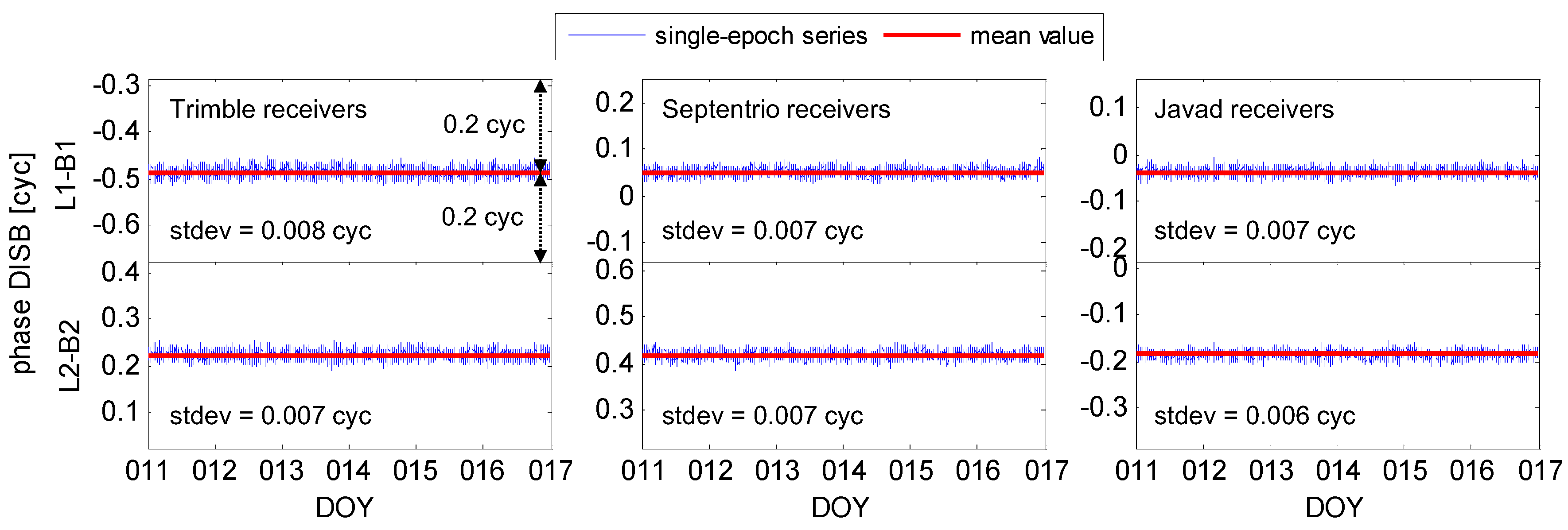
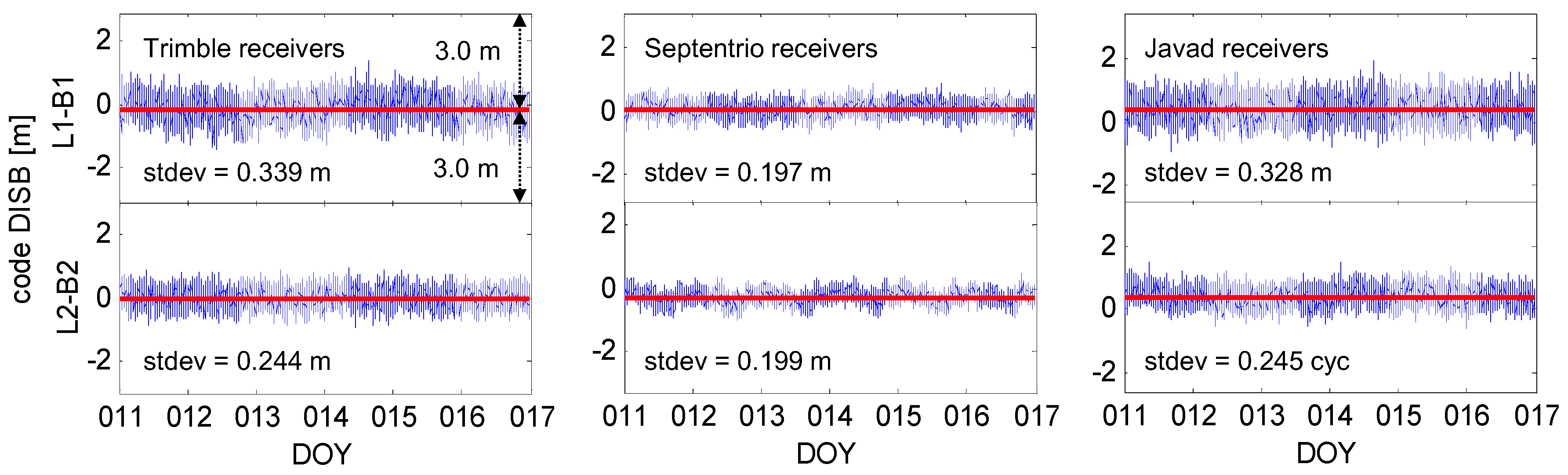
Figure 1 and Figure 2 depict the dual-frequency code and phase DISB time series, respectively, for the three baselines at Curtin University with the same receiver types. We can see, regardless of the random terms caused by observation noises, the DISBs estimators are very stable. The amplitudes relative to the mean value are all within 0.05 cycles, and the standard deviations (stdev) of the phase DISB estimators for both L1-B1 and L2-B2 are all within 0.008 cycles. The stdev of code DISBs estimators is much larger than those of the phase due to the pseudorange noise. However, a very stable trend can still be seen.

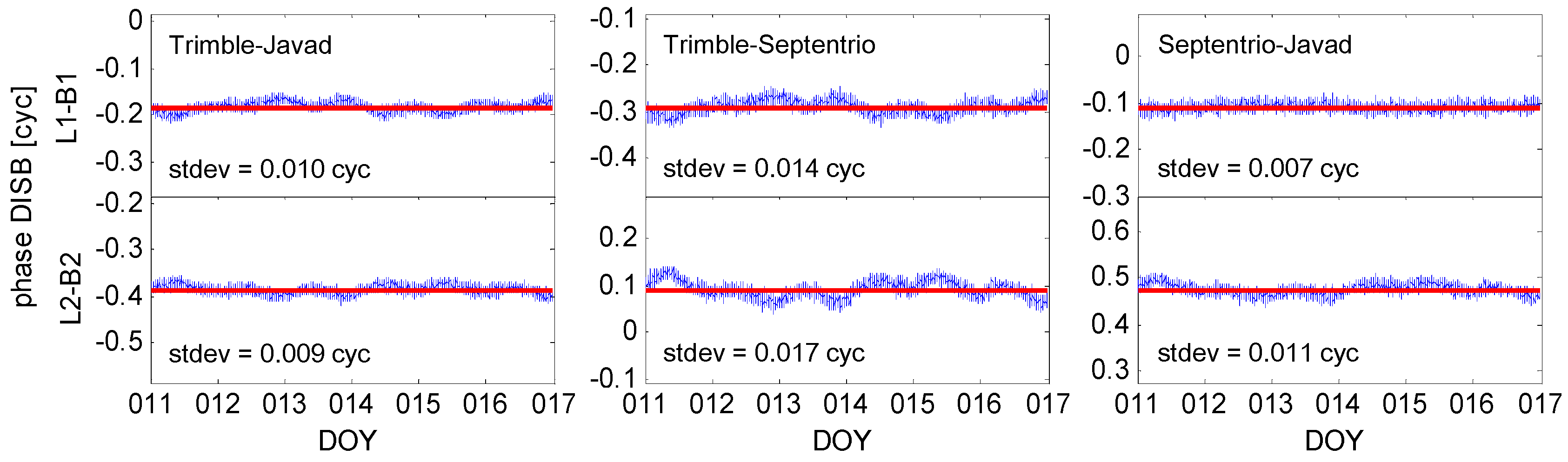
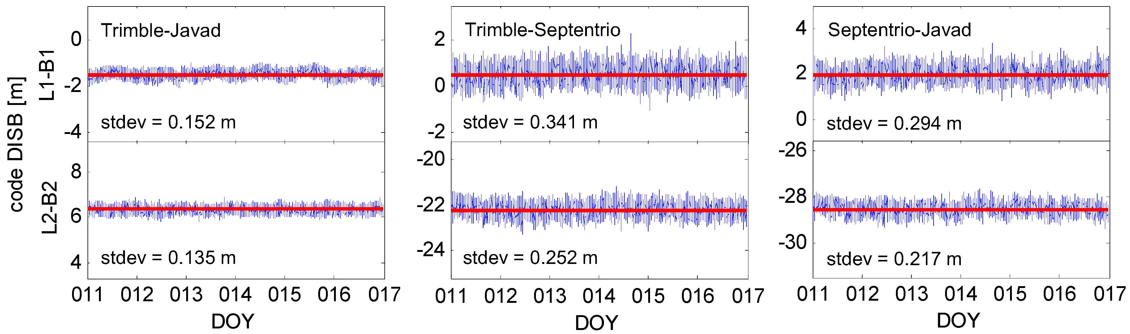
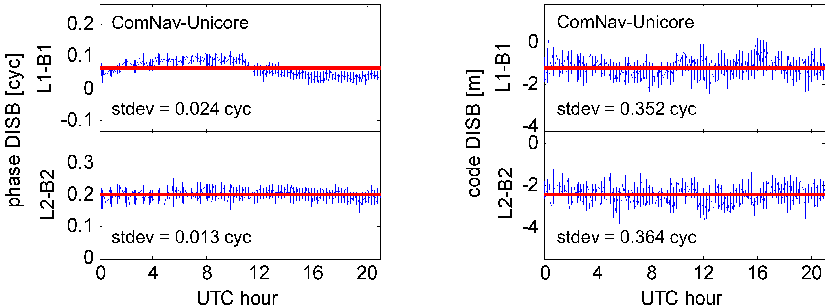
Figure 3 and Figure 4 depict the dual-frequency code and phase DISB series, respectively, for the three baselines at Curtin University with different receiver types. Figure 5 depicts the results for the baseline at Southeast University with receiver types of ComNav and Unicore. From these figures, we can see the code DISBs still appear generally stable with time. For the phase DISB series, besides the random terms, there are also small low-frequency variations (except Septentrio-Javad), even for the zero-baseline ‘CUT0-CUT1’ where no multipath effect exists. The standard deviations of the phase DISB estimators are obvious larger than those with the same receiver types. These low-frequency variations may be caused by the influence of different frequencies, since the inter-system differencing suffers not only the inter-system bias but the inter-frequency bias [33,34]. Fortunately, these variations are very slow and smooth. The amplitudes of the wave are all within about 0.1 cycle for tens of hours to several days. In the real-time estimation of GPS-BDS phase DISB, we can use the random walk process with a secure spectrum density (e.g., $0.05\times 0.05{\mathrm{cycle}}^2/\mathrm{h}$) to model this slow variation. This will also be utilized in the positioning experiments of next section.

4. Experiments of Medium-Baseline RTK Positioning

In this section, we mainly test the accuracy and reliability of combined GPS and BDS RTK positioning with the developed inter-system differencing model and classical differencing model. Two medium baselines CUT0-PERT and TG00-TGT0 were tested. The details of the two baselines can be seen in

Table 4. Information of the two medium baselines used in positioning experiments.

Baseline	Length/km	Duration	Sampling Interval	Receivers (Modules)	Location
CUT0-PERT	22.4 km	6 days (DOY 001–006, 2017)	30 s	Trimble NETR9	Perth, Australia
TG00-TGT0	75.9 km	20 h (UTC 4:00–24:00, DOY 23, 2016)	15 s	Trimble BD970	Tianjin, China

. The data of the baseline CUT0-PERT were downloaded from Multi-GNSS Experiment and Pilot Project (MGEX). The data of the baseline TG00-TG00 were collected in Tianjin, China.

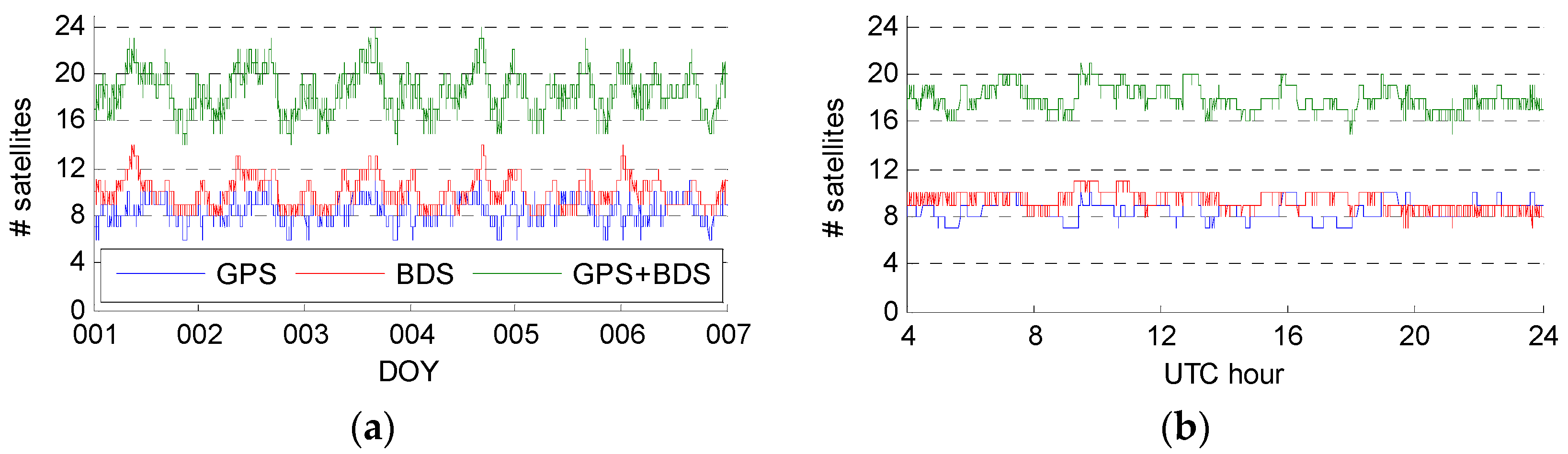
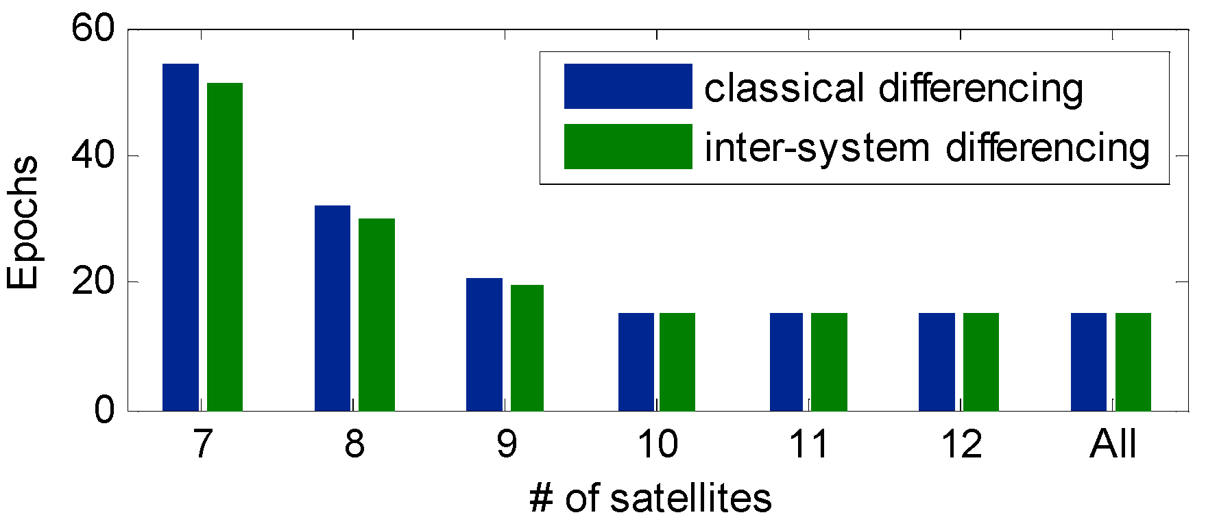
The numbers of the visible GPS and BDS satellites for the two baselines with a cut-off elevation of 10° are given in Figure 6. We can see with combined GPS and BDS, there are no less than 14 satellites available at all times for both the two baselines. In order to test the positioning performance with different satellite visibility, both of the positioning experiments below are carried out with 7–12 and all satellites, which are chosen in descending order of elevation.

4.1. Positioning Results of the 22.4-km Baseline

In the positioning tests, the initialization was carried out at the beginning of each day. Theoretically, real-time estimation of DISBs with characteristics of the slow time-variation is beneficial to both AR and positioning since additional redundancies are introduced. However, we find that the improvement for the AR in the RTK initialization period is very small. The average time to first fix (TTFF) of the two models with different visible satellites is shown in Figure 7. We can see that the TTFFs for the two models are very close, and just have small difference when a small number of satellites are visible. The reason is that in the initialization period, the DISB parameters with float ambiguities cannot achieve high precision, and thus only have small contribution to the convergence of ambiguities. However, once the ambiguities are correctly fixed for the first time, we can obtain the high-precision DISB estimators, and these will become useful information to strengthen the positioning model for the subsequent epochs.

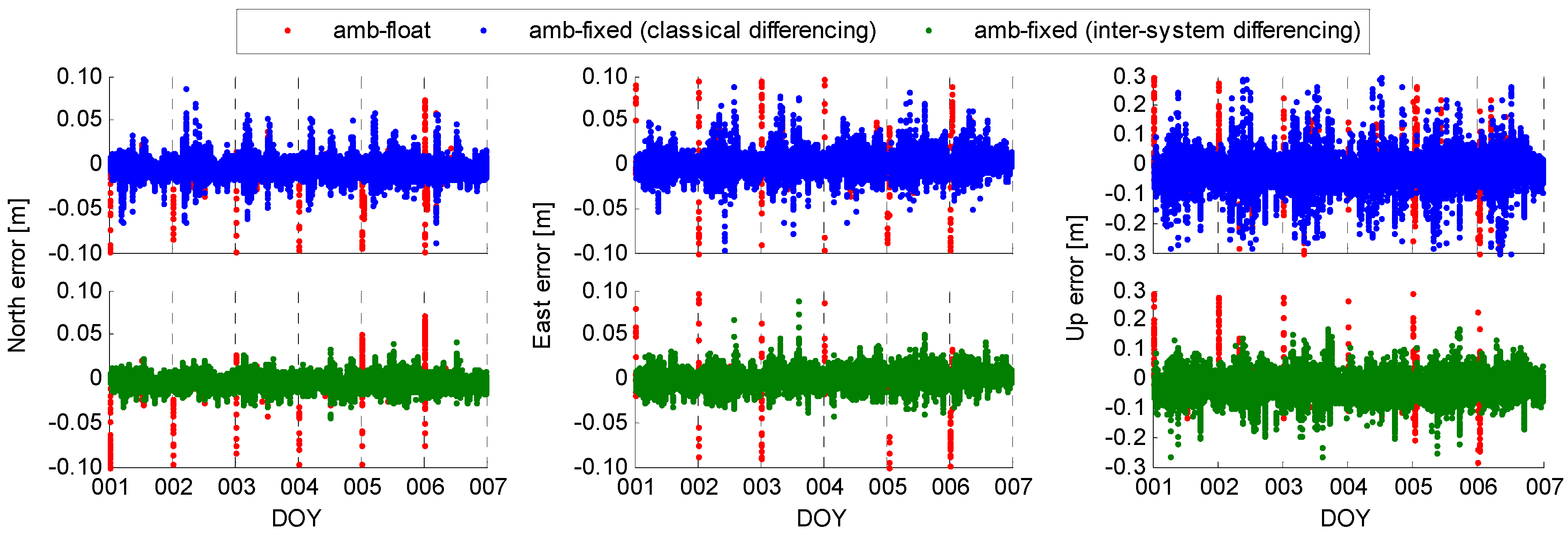
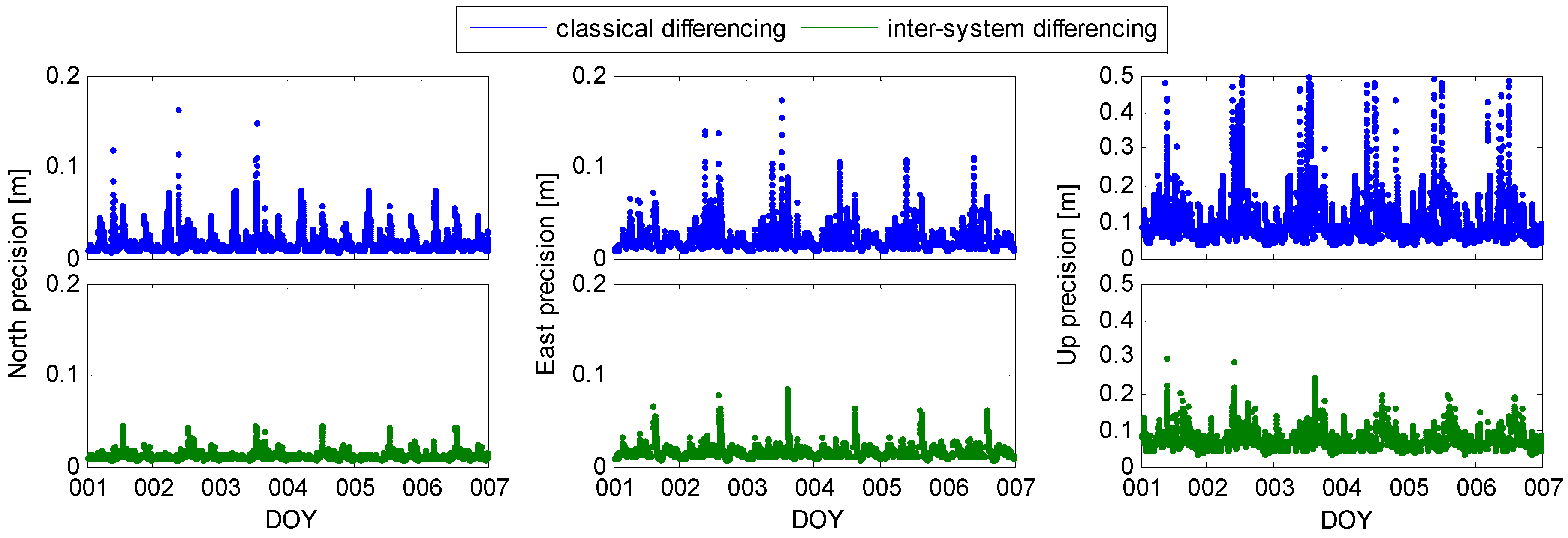
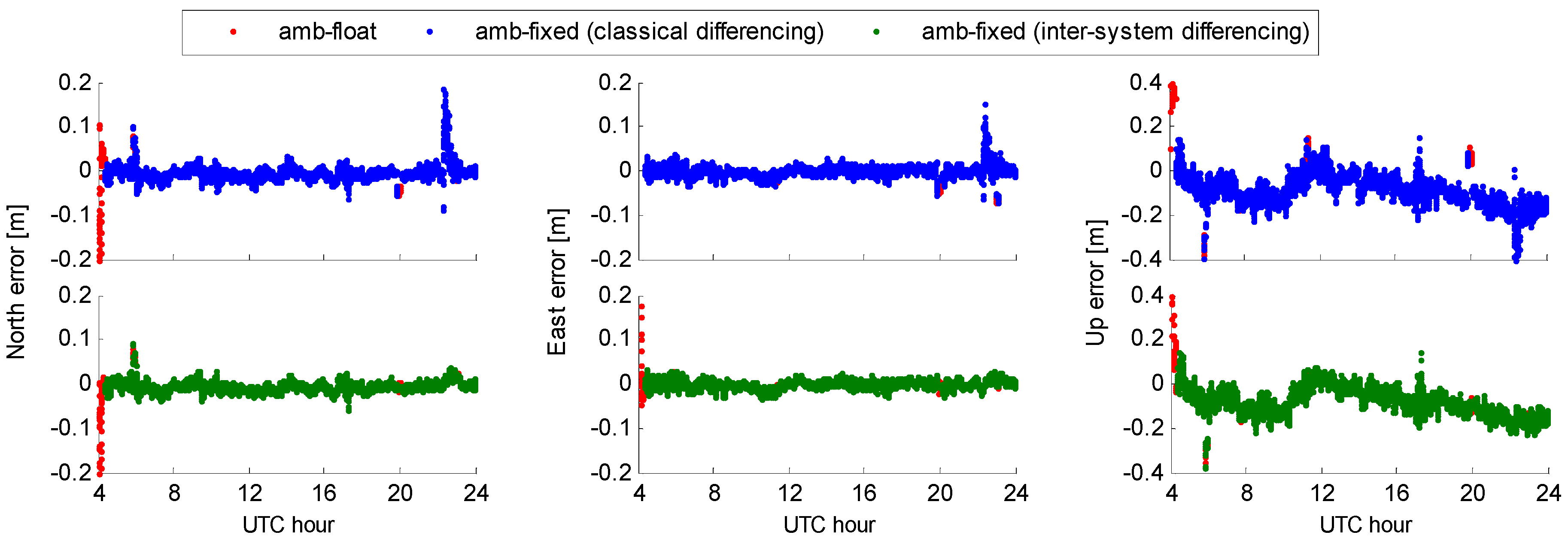
Figure 8 shows the positioning results with seven satellites for the 22.4-km baseline. The top three panels represent the results with the classical differencing model, while the bottom three represent the results with the inter-system differencing model. The positioning errors are obtained by comparing with the known coordinates. The initialization was carried out at the beginning of each day. On the whole, we can see that the ambiguity-fixed positioning results with the inter-system differencing model are more stable than those with the classical differencing model. The RMSs of positioning errors in North/East/Up directions are 1.07 cm/1.18 cm/6.96 cm for the classical differencing model. While for the inter-system differencing model, they are 0.81 cm/0.95 cm/4.59 cm, which represents an improvement of 23.9%/19.6%/34.1% in the three directions.

Figure 9 depicts the theoretical positioning precisions with ambiguity-fixed solutions for the two models, which are derived from the corresponding diagonal elements of the variance-covariance matrix at each epoch. Regardless of the actual observations, the theoretical positioning precisions can directly reflect the strength of the positioning model. We can see that at most times, the theoretical positioning precisions with the inter-system differencing model are obviously higher than those with the classical differencing model. This can also certify that the inter-system differencing model can strengthen the positioning model.

The RMSs of positioning errors with different number of visible satellites are listed in

Table 5. Positioning comparison for the classical differencing model and the inter-system differencing model with different numbers of visible satellites (22.4-km baseline).

Number of Satellites	RMSs of Positioning Errors (cm)						Improvement (%)
	Classical Differencing			Inter-System Differencing
	N	E	U	N	E	U	N	E	U
7	1.07	1.18	6.96	0.81	0.95	4.59	23.9	19.6	34.1
8	0.91	0.89	4.73	0.77	0.82	4.15	15.9	8.1	12.3
9	0.83	0.77	3.80	0.73	0.74	3.64	11.0	4.0	4.1
10	0.79	0.69	3.38	0.71	0.68	3.28	9.7	2.8	2.9
11	0.75	0.64	2.95	0.68	0.62	2.87	9.5	2.3	2.6
12	0.72	0.61	2.41	0.64	0.60	2.33	11.7	0.8	3.6
All	0.76	0.64	2.15	0.68	0.63	2.13	10.3	0.5	0.9

. These values are derived from the positioning errors by comparing with the known coordinates. We can see that as the number of visible satellites increases, the positioning performances become generally closer for the two models. Similar results were also derived, e.g., in the work by Paziewski and Wielgosz [35]. Anyway, the positioning performance with the inter-system differencing model is always better than that with the classical differencing model.

4.2. Positioning Results of the 75.9-km Baseline

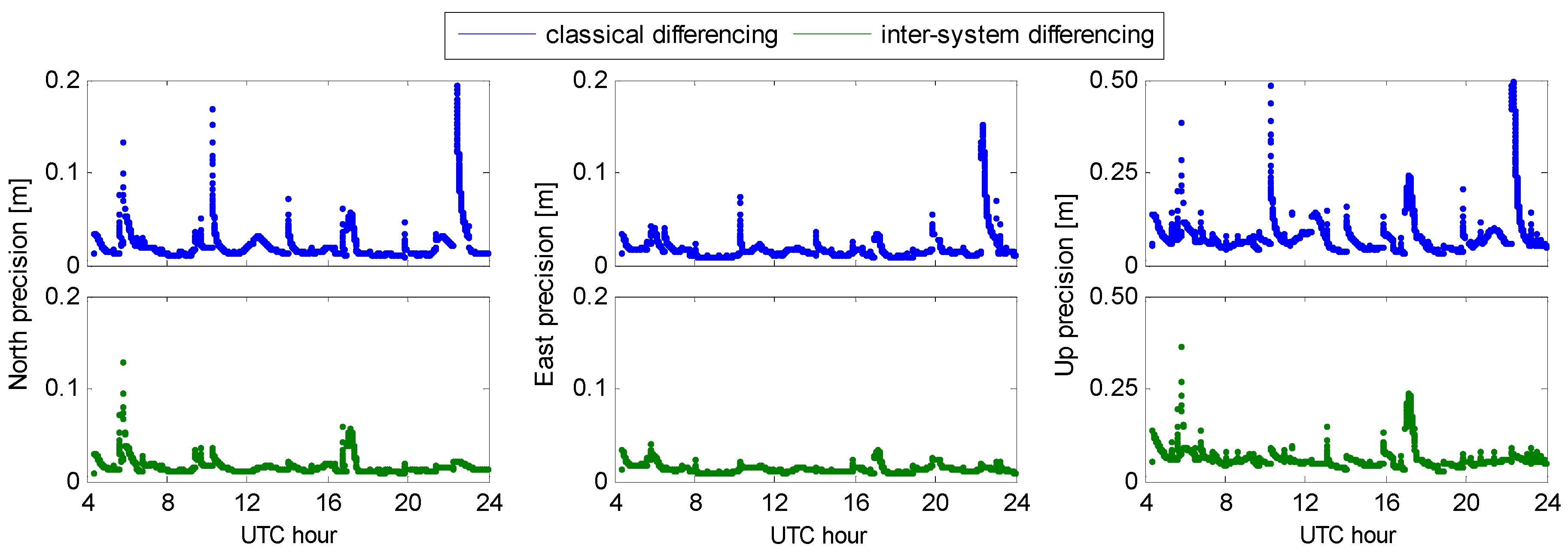
For the 75.9-km baseline, the RZTD parameter was estimated from epoch to epoch as a random-walk process. Figure 10 shows the positioning results with seven satellites. The top three panels represent the results with the classical differencing model, while the bottom three represent the results with the inter-system differencing model. We can see that, due to the longer baseline length and the introduction of the RZTD parameter, the positioning performance seems worse than that of the 22.4-km baseline, especially in the up direction. The RMSs of positioning errors in North/East/Up directions are 1.93 cm/1.33 cm/1.25 cm for the classical differencing model. While for the inter-system differencing model, they are 1.25 cm/0.96 cm/9.90 cm, which represents an improvement of 35.2%/27.6%/11.9% in the three directions. Particularly, during the period about 23:00–24:00, there are large fluctuations in the positioning errors with the classical differencing model. However, this phenomenon does not appear in the results with the inter-system differencing model. We have checked that the ambiguities are fixed correctly, and the reason is that the satellite geometry is poor in that period. This can also be seen in Figure 11, where we can see that the theoretical positioning precisions between 23:00 and 24:00 also present obvious differences for the two models. Similarly to Figure 9, at most times the theoretical positioning precisions with the inter-system differencing model are obviously better than those with the classical differencing model. The RMSs of positioning errors with different number of visible satellites for the 75.9-km baseline are listed in

Table 6. Positioning comparison for the classical differencing model and the inter-system differencing model with different numbers of visible satellites (75.9-km baseline).

Number of Satellites	RMSs of Positioning Errors (cm)						Improvement (%)
	Classical Differencing			Inter-System Differencing
	N	E	U	N	E	U	N	E	U
7	1.93	1.33	11.25	1.25	0.96	9.90	35.2	27.6	11.9
8	1.49	1.03	8.08	1.05	0.82	6.97	29.7	20.7	13.7
9	1.04	0.78	5.02	0.95	0.74	4.88	8.5	4.7	2.7
10	0.91	0.69	2.77	0.85	0.68	2.71	6.1	2.4	2.2
11	0.77	0.65	2.63	0.72	0.64	2.60	6.2	0.6	1.1
12	0.73	0.56	2.44	0.68	0.56	2.44	6.7	1.5	0.3
All	0.68	0.51	2.27	0.65	0.51	2.27	4.4	0.2	0.0

. Similarly, conclusions can be obtained from Table 5, namely that the positioning performances become closer for the two models as the number of visible satellites increases. The positioning performance with the inter-system differencing model is always better than or at least equivalent with that using the classical differencing model.

5. Discussion

In the proposed inter-system differencing model, the GPS-BDS DISBs are real-time estimated from epoch to epoch. Some recent contributions indicated that a priori calibration of DISBs led to better AR and positioning performance [11,13,14,15,35]. Indeed, between GPS L1-Galileo E1 and other cases with overlapping frequencies, the fractional phase DISB can be easily obtained from fixed integer ambiguities. If the DISBs are verified to be stable, they can be directly applied to calibrate subsequent calculation. However, when calculating phase DISB with different frequencies, the influence of between-receiver SD ambiguity of reference satellite cannot be separated from phase DISB unless the SD ambiguity can be calculated in advance. The SD ambiguity is usually calculated approximately using pseudoranges. The error of the SD ambiguity will directly introduce the bias for the phase DISB. What is more, even though the phase DISB are precisely calibrated, one also needs to face the problem of SD ambiguity again in the subsequent calculation. Only if the SD ambiguity is precisely solved, can the DD ambiguities be fixed to integers. Considering that the SD ambiguity is hard to solve precisely within a short time, we thus adopt the strategy of real time estimation.

Although the inter-system differencing model in this paper is proposed for relative RTK positioning, we think it can also be similarly used in the un-difference (UD) model, e.g., precise point positioning (PPP), as long as the UD inter-system biases are verified to be stable. In the UD model, one can estimate only one receiver clock parameter together with an ISB parameter between two systems. Then, the ISB parameter can be modelled with some constraints, e.g., as a constant or the random walk process, and thus the positioning performance could also be improved.

6. Conclusions

In this contribution, we studied the inter-system differencing between dual-frequency GPS and BDS for medium-baseline RTK positioning. The tightly combined ionosphere-free observation model with real-time estimation of DISBs was proposed. In the proposed model, the estimable ionosphere-free phase DISB is reparameterized to absorb not only the DD ambiguity between GPS and BDS reference satellites, but also the SD ambiguity of the GPS reference satellite. Thus, a full-rank inter-system differencing model can be obtained.

The stability of dual-frequency (i.e., L1-B1 and L2-B2) phase and code DISBs is analyzed using several baselines with the same or different receiver types. Our studies find that for the baselines with the same receiver types, both the phase and code DISBs are very stable. Although the phase DISBs may have small variations for different receiver types, fortunately, these variations are very slow and smooth. The amplitudes are within 0.1 cycles for tens of hours to several days. In practical use of the proposed inter-system differencing model, a random walk process with a secure spectrum density (e.g., $0.05\times 0.05{\mathrm{cycle}}^2/\mathrm{h}$) is recommended to model this slow variation.

Compared with the classical intra-system differencing model, although only the same number of DD ambiguities can be fixed to integers in the proposed model, the stability of the DISBs can still be used. Once the ambiguities are correctly fixed for the first time, we can obtain the high-precision DISB estimators. These high-precision DISB estimators will become useful information to strengthen the positioning model for the subsequent epochs, especially for obstructed environments with few visible satellites. Our experiments show that for the 22.4-km baseline and the 75.9-km baseline, when only seven satellites are available, the positioning accuracies in the three directions can be improved by 23.9%/19.6%/34.1% and 35.2%/27.6%/11.9%, respectively, with the proposed model. Generally, as the number of visible satellites increases, the positioning performances with the two models become closer. However, the proposed inter-system differencing model always outperformed (or was at least equivalent with) the classical differencing model.

References

- Ge, M.; Zhang, H.; Jia, X.; Song, S.; Wickert, J. What is Achievable with the Current COMPASS Constellation? In Proceedings of the 25th International Technical Meeting of the Satellite Division of the Institute of Navigation (ION GNSS 2012), Nashville, TN, USA, 17–21 September 2012. [Google Scholar]
- Odolinski, R.; Teunissen, P.J.G.; Odijk, D. Combined GPS + BDS + Galileo + QZSS for long baseline RTK positioning. In Proceedings of the ION GNSS 2014, Institute of Navigation, Tampa, FL, USA, 8–12 September 2014; pp. 2326–2340. [Google Scholar]
- Tegedor, J.; Øvstedal, O.; Vigen, E. Precise orbit determination and point positioning using GPS, Glonass, Galileo and BeiDou. J. Geod. Sci. 2014, 4, 65–73. [Google Scholar] [CrossRef]
- Geng, J.; Shi, C. Rapid initialization of real-time PPP by resolving undifferenced GPS and GLONASS ambiguities simultaneously. J. Geod. 2017, 91, 361–374. [Google Scholar] [CrossRef]
- Gao, W.; Gao, C.; Pan, S. A method of GPS/BDS/GLONASS combined RTK positioning for middle-long baseline with partial ambiguity resolution. Surv. Rev. 2017, 49, 212–220. [Google Scholar] [CrossRef]
- Teunissen, P.J.G.; Odolinski, R.; Odijk, D. Instantaneous BeiDou + GPS RTK positioning with high cut-off elevation angles. J. Geod. 2014, 88, 335–350. [Google Scholar] [CrossRef]
- Pan, S.; Meng, X.; Gao, W.; Wang, S.; Dodson, A. A new approach for optimizing GNSS positioning performance in harsh observation environments. J. Navig. 2014, 67, 1029–1048. [Google Scholar] [CrossRef]
- Liu, H.; Shu, B.; Xu, L.; Qian, C.; Zhang, R.; Zhang, M. Accounting for inter-system bias in DGNSS positioning with GPS/GLONASS/BDS/Galileo. J. Navig. 2017, 70, 686–698. [Google Scholar] [CrossRef]
- Gong, X.; Lou, Y.; Liu, W.; Zheng, F.; Gu, S.; Wang, H. Rapid ambiguity resolution over medium-to-long baselines based on GPS/BDS multi-frequency observables. Adv. Space Res. 2017, 59, 794–803. [Google Scholar] [CrossRef]
- Julien, O.; Alves, P.; Cannon, M.E.; Zhang, W. A tightly coupled GPS/GALILEO combination for improved ambiguity resolution. In Proceedings of the ENC GNSS 2003, Graz, Austria, 22–25 April 2003. [Google Scholar]
- Odijk, D.; Nadarajah, N.; Zaminpardaz, S.; Teunissen, P.J.G. GPS, Galileo, QZSS and IRNSS differential ISBs: Estimation and application. GPS Solut. 2016, 21, 439–450. [Google Scholar] [CrossRef]
- Tian, Y.; Ge, M.; Neitzel, F.; Zhu, J. Particle filter-based estimation of inter-system phase bias for real-time integer ambiguity resolution. GPS Solut. 2017, 21, 949–961. [Google Scholar] [CrossRef]
- Odolinski, R.; Teunissen, P.J.G.; Odijk, D. Combined BDS, Galileo, QZSS and GPS single-frequency RTK. GPS Solut. 2015, 19, 151–163. [Google Scholar] [CrossRef]
- Paziewski, J.; Wielgosz, P. Accounting for Galileo-GPS intersystem biases in precise satellite positioning. J. Geod. 2015, 89, 81–93. [Google Scholar] [CrossRef]
- Odijk, D.; Teunissen, P.J.G. Characterization of between-receiver GPS-Galileo inter-system biases and their effect on mixed ambiguity resolution. GPS Solut. 2013, 17, 521–533. [Google Scholar] [CrossRef]
- Nadarajah, N.; Khodabandeh, A.; Teunissen, P.J.G. Assessing the IRNSS L5-signal in combination with GPS, Galileo, and QZSS L5/E5a-signals for positioning and navigation. GPS Solut. 2015, 20, 289–297. [Google Scholar] [CrossRef]
- Li, G.; Wu, J.; Zhao, C.; Tian, Y. Double differencing within GNSS constellations. GPS Solut. 2017, 21, 1161–1177. [Google Scholar] [CrossRef]
- Lou, Y.; Gong, X.; Gu, S.; Zheng, F. An algorithm and results analysis for GPS+BDS inter-system mix double-difference RTK. J. Geod. Geodyn. 2016, 36, 1–5. [Google Scholar]
- Deng, C.; Tang, W.; Liu, J.; Shi, C. Reliable single-epoch ambiguity resolution for short baselines using combined GPS/BeiDou system. GPS Solut. 2014, 18, 375–386. [Google Scholar] [CrossRef]
- Böhm, J.; Möller, G.; Schindelegger, M.; Pain, G.; Weber, R. Development of an improved empirical model for slant delays in the troposphere (GPT2w). GPS Solut. 2015, 19, 433–441. [Google Scholar] [CrossRef]
- Li, B.; Feng, Y.; Shen, Y.; Wang, C. Geometry-specified troposphere decorrelation for subcentimeter real-time kinematic solutions over long baselines. J. Geophys. Res. 2010, 115, 1978–2012. [Google Scholar] [CrossRef]
- Melbourne, W. The case for ranging in GPS-based geodetic systems. In Proceedings of the 1st International Symposium on Precise Positioning with the Global Positioning System, Rockville, MD, USA, 15–19 April 1985; pp. 373–386. [Google Scholar]
- Wübbena, G. Software developments for geodetic positioning with GPS using TI-4100 code and carrier measurements. In Proceedings of the 1st International Symposium on Precise Positioning with the Global Positioning System, Rockville, MD, USA, 15–19 April 1985; pp. 403–412. [Google Scholar]
- Wang, G.; Jong, K.; Zhao, Q.; Hu, Z.; Guo, J. Multipath analysis of code measurements for BeiDou geostationary satellites. GPS Solut. 2015, 19, 129–139. [Google Scholar] [CrossRef]
- Wang, M.; Chai, H.; Liu, J.; Zeng, A. BDS relative static positioning over long baseline improved by GEO multipath mitigation. Adv. Space Res. 2016, 57, 782–793. [Google Scholar] [CrossRef]
- Li, B.; Shen, Y.; Feng, Y.; Gao, W.; Yang, L. GNSS ambiguity resolution with controllable failure rate for long baseline network RTK. J. Geod. 2014, 88, 99–112. [Google Scholar] [CrossRef]
- Teunissen, P.J.G.; Verhagen, S. The GNSS ambiguity ratio-test revisited: A better way of using it. Surv. Rev. 2009, 41, 138–151. [Google Scholar] [CrossRef]
- Takasu, T.; Yasuda, A. Kalman-filter-based integer ambiguity resolution strategy for long-baseline RTK with ionosphere and troposphere estimation. In Proceedings of the ION GNSS 2010, Institute of Navigation, Portland, OR, USA, 21–24 September 2010; pp. 161–171. [Google Scholar]
- Teunissen, P.J.G. The least-squares ambiguity decorrelation adjustment: A method for fast GPS integer ambiguity estimation. J. Geod. 1995, 70, 65–82. [Google Scholar] [CrossRef]
- Odijk, D.; Teunissen, P.J.G. ADOP in closed form for a hierarchy of multi-frequency single-baseline GNSS models. J. Geod. 2008, 82, 473–492. [Google Scholar] [CrossRef]
- Boehm, J.; Niell, A.; Tregoning, P.; Schuh, H. Global Mapping Function (GMF): A new empirical mapping function based on numerical weather model data. Geophys. Res. Lett. 2006, 33, L07304. [Google Scholar] [CrossRef]
- Eueler, H.J.; Goad, C.C. On optimal filtering of GPS dual frequency observations without using orbit information. Bull. Geod. 1991, 65, 130–143. [Google Scholar] [CrossRef]
- Sleewagen, J.; Simsky, A.; Wilde, W.D.; Boon, F.; Willems, T. Demystifying GLONASS Inter-Frequency Carrier Phase Biases; InsideGNSS: Eugene, OR, USA, 2012; Available online: http://www.insidegnss.com/auto/mayjune12-Sleewaegen.pdf (accessed on 13 September 2017).
- Geng, J.; Zhao, Q.; Shi, C.; Liu, J. A review on the inter-frequency biases of GLONASS carrier-phase data. J. Geod. 2017, 91, 329–340. [Google Scholar] [CrossRef]
- Paziewski, J.; Wielgosz, P. Investigation of some selected strategies for multi-GNSS instantaneous RTK positioning. Adv. Space Res. 2017, 59, 12–23. [Google Scholar] [CrossRef]
Figure 1.
L1-B1 and L2-B2 phase differential inter-system bias (DISB) time series for the three baselines at Curtin University with the same receiver types. The legend is the same for Figure 2, Figure 3, Figure 4 and Figure 5 below.
Figure 2.
L1-B1 and L2-B2 code DISB time series for the three baselines at Curtin University with the same receiver types.
Figure 3.
L1-B1 and L2-B2 phase DISB time series for the three baselines at Curtin University with different receiver types.
Figure 4.
L1-B1 and L2-B2 code DISB time series for the three baselines at Curtin University with different receiver types.
Figure 5.
L1-B1 and L2-B2 phase and code DISB time series for the baseline at Southeast University with receiver types of ComNav and Unicore.
Figure 6.
Number of GPS and BDS satellites for the two baselines with a cut-off elevation of 10°. (a) CUT0-PERT. (b) TG00-TGT0.
Figure 7.
The average time to first fix (TTFF) of the classical differencing model and the inter-system differencing model with different visible satellites.
Figure 8.
Positioning errors with seven satellites for the 22.4-km baseline with the classical differencing model and the inter-system differencing model. The vertical dot lines are the separation between consecutive initializations.
Figure 9.
The theoretical positioning precisions with ambiguity-fixed solutions for the 22.4-km baseline with the classical differencing model and the inter-system differencing model.
Figure 10.
Positioning errors with seven satellites for the 75.9-km baseline with the classical differencing model and the inter-system differencing model.
Figure 11.
The theoretical positioning precisions with ambiguity-fixed solutions for the 75.9-km baseline with the classical differencing model and the inter-system differencing model.